
Submitted:
21 October 2023
Posted:
23 October 2023
You are already at the latest version
Abstract
The World Meteorological Organization (WMO) recommends that the most recent 30-year period, i.e. 1991-2020, shall be used to compute climate normals of geophysical variables. A unique aspect this recent 30-year period is that the satellite-based observations of many different essential climate variables are available during this period, thus opening up new possibilities to provide a robust, global basis for the 30-year reference period in order to allow climate monitoring and climate change studies. Here, using the satellite-based climate data record of cloud and radiation properties, CLARA-A3, for the month of January between 1981 to 2020, we illustrate the difference between climate normal, as defined by guidelines from WMO on calculations of 30-yr climate normals, and climatology. It is shown that this difference is strongly dependent on the climate variable in question. We discuss the impacts of the nature and availability of satellite observations, variable definition, retrieval algorithm and programmatic configuration. It is shown that the satellite-based climate data records show enormous promise in providing climate normal for the recent 30-year period (1991-2020) globally. We finally argue that the holistic perspectives from the global satellite community should be increasingly considered while formulating the future WMO guidelines on computing climate normals.
Keywords:
climate normal
; climatology
; satellite remote sensing
; clouds and radiation
; climate change
; climate data records
; climate monitoring
; essential climate variables
; climate anomalies
; WMO
1. Introduction
The impacts of anthropogenic climate change are becoming increasingly vivid and tangible, affecting the bio-socio-economical fabric of all living organisms on our planet. The far-reaching implications of climate change mean that the need to assess the state of the climate becomes ever more important. What is the normal state of the climate? Which period can best represent the current state of the climate and be a reasonably good predictor for a near-future climate? Which basis shall be used for the near real time climate monitoring? The questions like these nowadays have real, practical socio-economic implications.
In light of these questions, the World Meteorological Organization (WMO) has provided guidelines to calculate climate normals of geophysical variables in the recent decades [1,2,3]. WMO recommends that the member states shall update their climate normals every decade with the most recent 30-year period finishing in a year ending with 0. This means that the latest 30-year normal period is considered to be 1991-2020. Previous studies have debated in detail if these latest normals can really be representative of the current climate or be a predictor for a near future one, given the rapid and non-linear changes ongoing in the climate system [4,5,6,7,8,9]. The economic implications of climate normals, for example in the energy sector, are also being discussed [10,11]. Even how to convey climate normals to the general public is far from being straightforward [12,13].
There are at least two important aspects that are worth discussing about this latest normal period.
a) The golden era of satellites: The latest normal period falls into the era wherein the space-based observations from both geostationary and polar orbiting satellites for a wide range of essential climate variables (ECVs), such as clouds, radiation, albedo, soil moisture, snow cover, humidity to name a few, are available [14,15]. The WMO climate normals have traditionally been geared towards the in-situ measurements of a few variables such as temperature and precipitation [1,2]. The satellite sensors now provide information on more than two-thirds of all ECVs and many of them do cover the entire 1991-2020 period [14,15]. Furthermore, there have been stratospheric improvements in the retrievals of ECVs in the recent decades, uplifting their quality and maturity to a level where climate data records of ECVs are being provided [16,17,18,19,20,21,22,23,24,25,26,27]. The satellite observations could also provide climate normals globally, going well beyond the limited area coverage by the in-situ measurements. The quality of reanalysis datasets has also been improving due to assimilation of better observations. Thus, in principle, the satellite-based climate data records and reanalysis could further complement one another to provide a global basis for climate normals.
b) Improved understanding of complex Earth system: The latest assessment reports from the Intergovernmental Panel on Climate Change (IPCC) outline the complexity of our Earth system and the feedbacks therein [28]. Our understanding of ECVs from the process to policy level has improved considerably in the last few decades. As we learn more and more about the importance of each climate variable in the Earth system, the demands for better information will increase from both the scientific community and the stakeholders. This means that in future the climate normals for many ECVs would be needed.
It is therefore clear that the satellite-based climate data records will play increasingly important role in defining climate normals for a wide array of ECVs in future. But computing climate normals from the climate data records is far from being easy and straightforward, and one needs also to understand how suitable and relevant WMO guidelines are for computing these normals. In the satellite community, the climatological averages provide the default basis to describe the state of the climate. The aim of this study, therefore, is to illustrate the difference between WMO climate normal and climatology for the same normal period using satellite-based climate data records. Here we focus on two key climate variables; cloud properties and incoming solar radiation at the surface. Cloud processes and feedbacks remain the largest source of uncertainty in climate models [29,30,31,32,33,34,35,36,37,38], while the information on incoming solar radiation is key to tackle future energy demands while transitioning to renewable energy [39,40,41,42,43,44] and for agricultural applications [45].
2. Satellite-based cloud and radiation climate data record
In this study, we use the data from the third edition of the CM SAF cLoud, Albedo and surface RAdiation dataset from AVHRR data, CLARA-A3 [21]. This climate data record has a rich history of dedicated, continuous developments and improvements dating back to its beginning 25 years ago in the framework of EUMETSAT’s Satellite Application Facility on Climate Monitoring [46]. CLARA-A3 provides the retrievals of global cloud fraction, cloud top and physical properties, surface albedo, and incoming surface solar radiation as well as the radiation at the top of the atmosphere. Furthermore, CLARA-A3 offers substantial improvements to its previous version, CLARA-A2. It employs cloud probabilistic detection based on the Naïve Bayesian theory, while the cloud top property algorithms employ artificial neural networks. A number of recent studies have documented the theoretical basis, validations and improvements in the CLARA-A3 climate data record [21,26,47,48,49].
In this study, we use both the Level 2b daily means and the Level 3 monthly means of cloud and radiation products that available at the 0.25 degree spatial resolution globally. The AVPOS flavour of this dataset is analysed here. This means that the Level 2b and Level 3 data are prepared using quality-controlled retrievals from AVHRR sensors flying onboard all available NOAA and MetOp satellites, instead of using only one prime morning or afternoon NOAA and MetOp satellite at a time. The CLARA-A3 CDR currently covers the period from 1979 to 2020 with an Interim, near-real time CDR thereafter. In this study, we evaluate different geophysical variables, namely total cloud fraction, daytime and nighttime cloud fraction, low cloud fraction, cloud top pressure, and incoming surface solar radiation.
3. Computation of climate normal and climatology
In 2017, WMO released its most recent guidelines on the computation of climatological normal (https://library.wmo.int/records/item/55797-wmo-guidelines-on-the-calculation-of-climate-normals). It details various aspects of data completeness, homogeneity, data precision and rounding relevant to computing climate normal [1]. This report, following the Guide to Climatological Practices, recommends that the individual monthly mean parameters based on the daily means shall not be calculated if any one of the following is true. a) The observations are missing for 11 or more days during the month, hereafter referred to as the D11 condition; b) Observations are missing for a period of 5 or more consecutive days during the month, hereafter referred to as the D5 condition. The report further recommends that, for a normal or average to be calculated for a given month, data should be available for at least 80% of the years in the averaging period. This equates to having data available for that month in 24 or more out of the 30 years for a climatological standard normal or a reference normal.
In this study, we computed two different versions of climate normal and two different climatologies for the geophysical variables mentioned in Section 2. The rationale and methodology behind these normals and climatologies are explained below.
CN_WMO: This refers to the “true climate normal” computed by adhering to all three WMO recommendations on daily and monthly data completeness mentioned above. In practice, this is done as follows. Using the daily means of a geophysical variable in question available at Level 2b, we created flags for each 0.25 degree lat-lon grid that satisfy D5 and/or D11 condition for each month during the 1991-2020 period. We then computed the mean parameter for those grids that satisfy both D5 and D11 conditions and have data available for at least 24 of the 30 years. We refer to this version of climate normal as CN_WMO because it strictly follows all WMO guidelines on data completeness.
CN_MB: This refers to the climate normal computed only using Level 3 monthly mean data. This is a straightforward and easy-to-provide version of the climate normal. In practice, this means that we apply a basic quality control on the Level 3 data and compute mean parameter if the data are available for at least 24 of the 30 years.
Clim30: This refers to the 30-year arithmetic climatological average for the 1991-2020 period without applying any condition on data completeness on the daily or the monthly means. Such climatological averages are often used for climate monitoring, climate change studies, to provide climate anomalies and to study the impact of extreme events. In principle, if the satellite observations are continuous and are of good quality throughout the 30-year period, CN_WMO, CN_MB and Clim30 would be exactly identical.
Clim40: This refers to the extended 40-year climatological average for the 1981-2020 period. It is possible to calculate this extended climatological average, since the CLARA-A3 climate data record extends back 42 years to 1979. By comparing CN_WMO with Clim30 and Clim40, the readers could get an idea about the impact of having 10 extra years of observations.
In the sections below, the difference between these climate normals and climatologies is illustrated for the month of January as a demonstrative and feasibility case study.
4. Difference between climate normals and climatologies
4.1. Total and low cloud fraction
Figure 1 shows the absolute values of climate normal of total cloud fraction for the month of January following the strict WMO data completeness guidelines (i.e. CN_WMO) together with the differences between CN_WMO and the other versions of climate normal and climatologies as explained in Section 3 above. It can be seen that, in the case of total cloud fraction, the CN_WMO, CN_MB and Clim30 are exactly identical. This means that the conventional 30-year climatology can fully represent climate normal for this variable in question. This is possible mainly due to the fact that the total cloud fraction is retrieved under all circumstances wherein the quality controlled data are available, which has predominantly been the case during the 1991-2020 period. This is evident in Figure 2 which shows the total number of longitude grid points failing either the D5 or the D11 condition in the latitude-time domain. In 1995 a brief data loss occurred during the change from NOAA-11 to NOAA-14 satellite platform. The availability of NOAA-12 during this time was not enough at the higher latitudes in the northern hemisphere to cover the data loss due to the change of satellite platform and the data loss due to solar contamination of thermal channels [50,51]. However, in all other years, the valid daily means are available continously and uniformly, thus allowing the computation of CN_WMO globally.
When the total cloud fraction is sub-divided into contributions from low, middle and high clouds, CN_WMO, CN_MB and Clim30 are also exactly identical. This is shown in Figure 3 in the case of low cloud fraction. This shows that all valid outcomes of cloud detection lead to the successful classification into low, middle or high cloud types. This data completeness further enables the successful computation of CN_WMO. Similar results also apply for the middle and high clouds (not shown here).
The differences between CN_WMO and Clim40 shown in Figure 1 and Figure 3 for the total and low cloud fraction respectively are noteworthy. Previous studies have shown that the global cloud cover is generally decreasing over the course of last fourty years [21,23,25,26,48]. This decrease has mainly occurred over the sub-tropical to mid-latitudes in both hemispheres. It is however worth pointing out that this decrease has not been continuous throughout the 40-year period (1981-2020). The global mean cloudiness has in fact been increasing in the last two decades that dominate the most recent climate normal period. Since Clim40 includes extra 10 years of data from the decade before the lastest normal period (1991-2020) when the cloud cover was higher, the global mean differences between CN_WMO and Clim40 are still negative. There are however some regions where these differences are positive due to increasing trends in cloudiness, for example, the stratocumulus regions in the southeast Pacific off the northwestern coast of South America and also the stratocumulus region in the southeast Atlantic. This is especially evident in Figure 3. It should be noted that these regions are strongly influenced by the El Nino Southern Oscillation (ENSO) and even this extended 40-year climatology may not be long enough to fully cover the variability associated ENSO, as argued in the previous studies. These results illustrate why a more cautionary approach is required when assessing the state of the climate based on the most recent climate normal period.
4.2. Daytime and nighttime cloud fraction
Figure 4 and Figure 5 show the similar results as in Figure 1, but for the daytime and nighttime cloud fractions respectively. Here, the differences between CN_WMO and the other variants of climatologies are clearly evident. The global mean daytime cloud fraction in CN_WMO is 0.62% and 0.79% lower compared to CN_MB and Clim30 respectively (Figure 4). The differences are much stronger locally and can even have different signs. Furthermore, CN_WMO could not be computed over the polar region in the northern hemisphere extending as south as 45 degrees latitude.
In order to understand this data gap in CN_WMO and the differences against CN_MB and Clim30, one has to first note the definition of daytime cloud fraction in the CLARA-A3 climate data record. When the local solar zenith angles are less than 75 degrees, it is considered to be the daytime condition and when they are larger than 95 degrees, it is considered to be the nighttime. Since the sun remains below the horizon in the Arctic in January, there is natural data gap resulting in the Arctic, as visible in the Clim30 case in Figure 6 that shows the total number of years used to compute CN_WMO and Clim30, and the difference thereof. But the data gap in CN_WMO extends even more southward to 45 degrees north. This is due to the fact that, in the latitude band between 45⁰N and 55⁰N, the solar zenith angle decreases every day throughout the January month, but remains below 75⁰ in the first half of January. This means that the D5 and D11 conditions are not satisfied in this latitude band as shown in Figure 7, resulting in the data gap.
The computation of CN_WMO is further influenced by the orbital drift of NOAA satellites [52]. For example, the afternoon NOAA satellites have drifted significantly from their sun-synchronous orbits causing increasingly delayed local observational times. The orbital drift can affect the paritioning among daytime, twilight and nighttime conditions more strongly at the higher latitudes during polar winters since the daily rate of change of solar zenith angle is higher there and just a few hours delay in the local observational times can cross over the daytime threshold for solar zenith angles. This is also clearly evident in Figure 7 between the latitude bands 30⁰N to 45⁰N between 1991 and 2000 when the data from fewer satellites was available and the NOAA-11 (1991-1995) and NOAA-14 (1995-2000) drifted considerably towards the end of their lifespans. This resulted in the gradual loss of data, spatially extending even more southwards towards the later years of their life. Figure 7 further shows that the data loss in the case of daytime cloud fraction due to ortibal drift has not been uniform over the rest of the globe. This inadequate sampling together with different diurnal cycles of various cloud regimes lead to different signs of the difference between CN_WMO and Clim30 in Figure 4.
It is also to be noted that in the latter two decades (2001-2020), the data from multiple NOAA and MetOp satellites are available to compute daytime cloud fraction, thus the impact of orbital drift of an individual satellite is not clearly visible anymore during this period.
Similar conclusions can also be applied to the climate normals of nighttime cloud fraction shown in Figure 5, execept in this case, it is the southern polar regions that are affected by the problems associated with the orbital drift and solar zenith angles as well as the solar contamination in the thermal channels.
Another interesting feature to note in Figure 4 and Figure 5 is the global mean diferrence between CN_WMO and Clim40. This difference is much stronger in the case of nighttime cloud fraction compared to its daytime counterpart. It is due to the fact that this difference is driven mainly by the strong decreases in mid- to high latitude clouds over the oceans during nighttime, while, in the case of daytime, the increases in low level oceanic stratocumulus clouds in the southern hemisphere dampen this difference. These results presented in Figure 4, Figure 5, Figure 6 and Figure 7 show the compleixity of the situation and the sensitivity of CN_WMO computation to various factors such as variable definition, and orbital and programmatic configurations.
4.3. Cloud top pressure
Figure 8, Figure 9 and Figure 10 show the similar results as in Figure 4, Figure 6 and Figure 7, but for the cloud top pressure. Here, we note that CN_WMO could not be computed over the desert regions in the tropics as well as over the parts of Greenland and Antarctica. There are also some differences between CN_WMO and Clim30 over other regions peripheral to these data gaps. These gaps in climate normals of cloud top pressure can be explained by the following factors. First and foremost, it is physically possible that, in the desert regions and few other tropical regions, clouds may not develop every day and clear sky conditions could prevail for longer times within a month. This is especially the case during the drier summer and winter months. This means that the D5 and/or D11 conditions are not satisfied in practice, since the cloud top pressures are naturally retrieved only when clouds are present. It is therefore clear that the WMO guidelines are not suitable in this case.
The situation over the Antarctic and Greenland is even more interesting. Here, the data gaps in climate normals are not just due to the prevailing clear sky conditions, but also due to the fact that the cloud detection algorithm in CLARA-A3 may miss clouds over the bright and cold polar regions, especially in cases of extremely cold surface temperatures [21,48], and then no other cloud properties are retrieved downstream. This shows that the cloud detection sensitivity of climate data records could also play an important role while computing the climate normals. The spatial features in the data gaps in Figure 9 and Figure 10 support these explanations. The impact of orbital drift is also seen in Figure 10 in the northern hemispheric dry belt (10N-30N) when the number of longitude grid points fulfilling the D5 and D11 conditions increase gradually in the first decade when NOAA-11 (1991-1995) and NOAA-14 (1995-2000) satellites were active.
Another noticeable feature in Figure 8 is that the difference between CN_WMO and Clim30 is exactly identical to the difference between CN_WMO and CN_MB. This means that the climate normals based only on the monthly mean data are exactly identical to the 30-year climatology. The data gaps in CN_WMO are driven mainly by the fulfilment of the D5 and D11 conditions that are applied to the daily means and are not relevant to CN_MB. This further means that no added benefit is obtained by computing the climate normals based only on monthly means compared to the respective 30-year climatology.
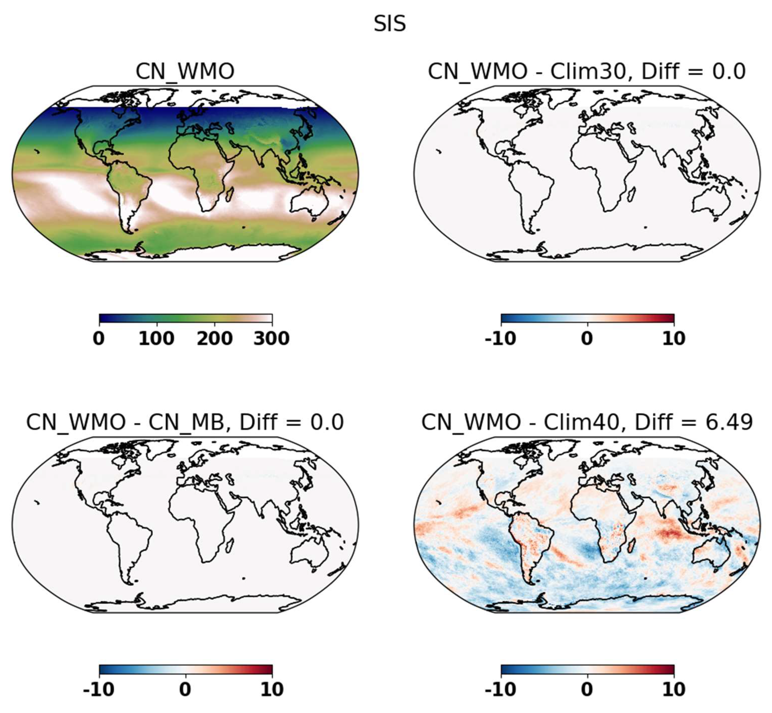
4.4. Incoming solar radiation at the surface (SIS)
Figure 11 shows the true climate normals of SIS and the differences with respect to CM_MB, Clim30 and Clim40. Similar to the results shown for total cloud fraction before, there are no differences between CN_WMO, CN_MB and Clim30. This shows the progress made in data completeness both at the Level 2 daily and Level 3 monthly mean levels in the CLARA-A3 climate data record. An interesting feature to note here is that the difference between CN_WMO and Clim40 for SIS correlates well with the similar difference for the daytime and low level cloud fractions shown before. For example, those regions located off the western coasts of South America and southern Africa where the stratocumulus clouds show statistically significant increases, the incoming surface solar radiation has correspondingly decreased in the latter 30-year period compared to Clim40. An opposite feature can be observed in the Indian Ocean.
5. Conclusions
We illustrated the difference between a climate normal and a climatology using a satellite-based climate data record globally. Since the latest climate normal period (1991-2020) falls entirely in the satellite era, it opens up new opportunities to compute climate normals of many different essential climate variables, going well beyond the normals usually computed using in-situ measurements for a limited number of variables such as temperature and precipitation. Furthermore, the recent advances in data rescue, better calibration, improved retrieval algorithms and data completeness mean that the satellite-based climate data records are becoming increasingly suitable for computing climate normals at a global scale.
In this demonstrative study, we applied the WMO guidelines on data completeness while computing climate normals of various cloud properties and incoming surface solar radiation provided in the CLARA-A3 climate data record. We have shown that for certain variables, such as total cloud fraction and surface solar radiation, the climate normals and climatologies are practically identical during the most recent 30-year period (1991-2020). This shows the benefits data completeness in the recent satellite era.
However, for other variables, such as daytime and nighttime cloud fractions, that are defined using a particular threshold on solar zenith angles, the guidelines on data completeness while computing the monthly mean parameter could be difficult to fulfil in the mid- to higher latitude regions. This is simply due to the fact that the daily changes in the solar zenith angles over these regions are stronger than those in the equatorial regions. In these cases, the climate normals based only on monthly data are the same as climatologies and both of them differ significantly from the true climate normals. This means that no significant gains are obtained by computing only monthly based climate normals. It is to be noted that these conclusions could also apply to other variables such as cloud microphysical properties (cloud optical depth, effective radius, water path etc) that are also retrieved under certain solar illumination conditions.
The situation is even more complex for some of the other variables such as cloud top properties that are retrieved only in the presence of clouds. There are many regions on Earth where clouds can be absent for more than 5 days in a row or for more than 11 days in total in a given month. Over these regions, which are located mainly in the tropical dry belt and Antarctica, the D5 and/or D11 conditions are not fulfilled, thus leading to gaps in climate normals.
It is clear that a wider discussion about the suitability of WMO guidelines in the satellite era is needed to extend them in future to account for different physical conditions pertaining to different climate variables derived from satellite-based observations. For example, similar difficulties could also arise when computing climate normals for aerosol properties, trace gases, surface temperatures etc, where limited clear-sky conditions and cloud detection sensitivity could influence the fulfilment of the D5 and/or D11 conditions. The impact of clear-sky biases on climate normals of these variables also needs to be understood globally.
In spite of some local data gaps, the satellite-based climate data records show a good promise for computing climate normals globally. Having both the increasingly detailed and the holistic perspectives from the satellite community could help enormously to better formulate future WMO guidelines on climate normals.
Author Contributions
Conceptualization, A. D.; formal analysis, A. D.; investigation, A.D.; writing—original draft preparation, A. D.; writing—review and editing, A. D., S. A., K-G. K., E. E.; visualization, A. D.; project administration, A. D., S. A., E. E.; funding acquisition, A. D., E. E., K-G. K. All authors have read and agreed to the published version of the manuscript.
Funding
This research was funded by Swedish Research Council grant number 2021-05143 and the Swedish Government’s 2023 Climate Adaptation Grant 1:10 to SMHI.
Data Availability Statement
The CLARA-A3 dataset is publicly available through: https://doi.org/10.5676/EUM_SAF_CM/CLARA_AVHRR/V003.
Acknowledgments
The authors acknowledge the EUMETSAT member states for supporting EUMETSAT’s CM SAF. .
Conflicts of Interest
The authors declare no conflict of interest. The funders had no role in the design of the study; in the collection, analyses, or interpretation of data; in the writing of the manuscript; or in the decision to publish the results.
References
- WMO Guidelines on the calculation of climate normals, WMO-No. 1203, 2017 Edition, pp. 1-18. Geneva.
- WMO Guide to Climatological Practices (WMO-No. 100). 2011. Geneva.
- WMO The Role of Climatological Normals in a Changing Climate (WMO/TD-No. 1377). 2007. Geneva.
- Arguez, A.; Vose, R.S. The Definition of the Standard WMO Climate Normal: The Key to Deriving Alternative Climate Normals. Bull. Am. Meteorol. Soc. 2011, 92, 699–704. [Google Scholar] [CrossRef]
- Livezey, R.E.; Vinnikov, K.Y.; Timofeyeva, M.M.; Tinker, R.; Dool, H.M.v.D. Estimation and Extrapolation of Climate Normals and Climatic Trends. J. Appl. Meteorol. Clim. 2007, 46, 1759–1776. [Google Scholar] [CrossRef]
- Rigal, A.; Azaïs, J.-M.; Ribes, A. Estimating daily climatological normals in a changing climate. Clim. Dyn. 2019, 53, 275–286. [Google Scholar] [CrossRef]
- Steinacker, R. How to correctly apply Gaussian statistics in a non-stationary climate? Theor. Appl. Clim. 2021, 144, 1363–1374. [Google Scholar] [CrossRef]
- Wilks, D.S. Projecting “Normals” in a Nonstationary Climate. J. Appl. Meteorol. Clim. 2013, 52, 289–302. [Google Scholar] [CrossRef]
- Holder, C.; Boyles, R.; Robinson, P.; Raman, S.; Fishel, G. Calculating A Daily Normal Temperature Range That Reflects Daily Temperature Variability. Bull. Am. Meteorol. Soc. 2006, 87, 769–774. [Google Scholar] [CrossRef]
- Won, S.J.; Wang, X.H.; Warren, H.E. Climate normals and weather normalization for utility regulation. Energy Econ. 2016, 54, 405–416. [Google Scholar] [CrossRef]
- Arguez, A.; Vose, R.S.; Dissen, J. Alternative Climate Normals: Impacts to the Energy Industry. Bull. Am. Meteorol. Soc. 2013, 94, 915–917. [Google Scholar] [CrossRef]
- Gent, P.R. Climate Normals: Are They Always Communicated Correctly? Weather. Forecast. 2022, 37, 1531–1532. [Google Scholar] [CrossRef]
- Lupo, A. R. , and Coauthors. The presentation of temperature information in television broadcasts: What is normal? Natl. Wea. Dig. 2003, 27, 53–58. [Google Scholar]
- Bojinski, S.; Verstraete, M.; Peterson, T.C.; Richter, C.; Simmons, A.; Zemp, M. The Concept of Essential Climate Variables in Support of Climate Research, Applications, and Policy. Bull. Am. Meteorol. Soc. 2014, 95, 1431–1443. [Google Scholar] [CrossRef]
- Popp, T.; Hegglin, M.I.; Hollmann, R.; Ardhuin, F.; Bartsch, A.; Bastos, A.; Bennett, V.; Boutin, J.; Brockmann, C.; Buchwitz, M.; et al. Consistency of Satellite Climate Data Records for Earth System Monitoring. Bull. Am. Meteorol. Soc. 2020, 101, E1948–E1971. [Google Scholar] [CrossRef]
- Rossow, W.B. 2022: History of the International Satellite Cloud Climatology Project. WCRP Report 6/2022; World Climate Research Programme (WCRP): Geneva, Switzerland, 2022; p. 87. [Google Scholar] [CrossRef]
- Schiffer, R.A.; Rossow, W.B. The International Satellite Cloud Climatology Project (ISCCP): The First Project of the World Climate Research Programme. Bull. Am. Meteorol. Soc. 1983, 64, 779–784. [Google Scholar] [CrossRef]
- Heidinger, A.K.; Foster, M.J.; Walther, A.; Zhao, X. (. The Pathfinder Atmospheres–Extended AVHRR Climate Dataset. Bull. Am. Meteorol. Soc. 2013, 95, 909–922. [Google Scholar] [CrossRef]
- Karlsson, K.-G.; Anttila, K.; Trentmann, J.; Stengel, M.; Meirink, J.F.; Devasthale, A.; Hanschmann, T.; Kothe, S.; Jääskeläinen, E.; Sedlar, J.; et al. CLARA-A2: the second edition of the CM SAF cloud and radiation data record from 34 years of global AVHRR data. Atmos. Chem. Phys. 2017, 17, 5809–5828. [Google Scholar] [CrossRef]
- Stengel, M.; Stapelberg, S.; Sus, O.; Schlundt, C.; Poulsen, C.; Thomas, G.; Christensen, M.; Henken, C.C.; Preusker, R.; Fischer, J.; et al. Cloud property datasets retrieved from AVHRR, MODIS, AATSR and MERIS in the framework of the Cloud_cci project. Earth Syst. Sci. Data 2017, 9, 881–904. [Google Scholar] [CrossRef]
- Karlsson, K.-G.; Stengel, M.; Meirink, J.F.; Riihelä, A.; Trentmann, J.; Akkermans, T.; Stein, D.; Devasthale, A.; Eliasson, S.; Johansson, E.; et al. CLARA-A3: The third edition of the AVHRR-based CM SAF climate data record on clouds, radiation and surface albedo covering the period 1979 to 2023. Earth Syst. Sci. Data 2023, 15, 4901–4926. [Google Scholar] [CrossRef]
- Stengel, M.; Stapelberg, S.; Sus, O.; Finkensieper, S.; Würzler, B.; Philipp, D.; Hollmann, R.; Poulsen, C.; Christensen, M.; McGarragh, G. Cloud_cci Advanced Very High Resolution Radiometer post meridiem (AVHRR-PM) dataset version 3: 35-year climatology of global cloud and radiation properties. Earth Syst. Sci. Data 2020, 12, 41–60. [Google Scholar] [CrossRef]
- Foster, M.J.; Phillips, C.; Heidinger, A.K.; Borbas, E.E.; Li, Y.; Menzel, W.P.; Walther, A.; Weisz, E. PATMOS-x Version 6.0: 40 Years of Merged AVHRR and HIRS Global Cloud Data. J. Clim. 2022, 36, 1143–1160. [Google Scholar] [CrossRef]
- Young, A.H.; Knapp, K.R.; Inamdar, A.; Hankins, W.; Rossow, W.B. The International Satellite Cloud Climatology Project H-Series climate data record product. Earth Syst. Sci. Data 2018, 10, 583–593. [Google Scholar] [CrossRef]
- Karlsson, K.-G.; Devasthale, A. Inter-Comparison and Evaluation of the Four Longest Satellite-Derived Cloud Climate Data Records: CLARA-A2, ESA Cloud CCI V3, ISCCP-HGM, and PATMOS-x. Remote. Sens. 2018, 10, 1567. [Google Scholar] [CrossRef]
- Devasthale, A.; Karlsson, K.-G. Decadal Stability and Trends in the Global Cloud Amount and Cloud Top Temperature in the Satellite-Based Climate Data Records. Remote. Sens. 2023, 15, 3819. [Google Scholar] [CrossRef]
- Stubenrauch, C.J.; Rossow, W.B.; Kinne, S.; Ackerman, S.; Cesana, G.; Chepfer, H.; Di Girolamo, L.; Getzewich, B.; Guignard, A.; Heidinger, A.; et al. Assessment of Global Cloud Datasets from Satellites: Project and Database Initiated by the GEWEX Radiation Panel. Bull. Am. Meteorol. Soc. 2013, 23, 1031–1049. [Google Scholar] [CrossRef]
- IPCC, 2021: Climate Change 2021: The Physical Science Basis. Contribution of Working Group I to the Sixth Assessment Report of the Intergovernmental Panel on Climate Change [Masson-Delmotte, V., P. Zhai, A. Pirani, S.L. Connors, C. Péan, S. Berger, N. Caud, Y. Chen, L. Goldfarb, M.I. Gomis, M. Huang, K. Leitzell, E. Lonnoy, J.B.R. Matthews, T.K. Maycock, T. Waterfield, O. Yelekçi, R. Yu, and B. Zhou (eds.)]. Cambridge University Press, Cambridge, United Kingdom and New York, NY, USA, 2391 pp.
- Bony, S.; Dufresne, J. Marine boundary layer clouds at the heart of tropical cloud feedback uncertainties in climate models. Geophys. Res. Lett. 2005, 32. [Google Scholar] [CrossRef]
- Stephens, G.L. Cloud Feedbacks in the Climate System: A Critical Review. J. Clim. 2005, 18, 237–273. [Google Scholar] [CrossRef]
- Zelinka, M.D.; Zhou, C.; Klein, S.A. Insights from a refined decomposition of cloud feedbacks. Geophys. Res. Lett. 2016, 43, 9259–9269. [Google Scholar] [CrossRef]
- Cesana, G.V.; Del Genio, A.D. Observational constraint on cloud feedbacks suggests moderate climate sensitivity. Nat. Clim. Chang. 2021, 11, 213–218. [Google Scholar] [CrossRef]
- Ceppi, P.; Nowack, P. Observational evidence that cloud feedback amplifies global warming. Proc. Natl. Acad. Sci. 2021, 118, e2026290118. [Google Scholar] [CrossRef]
- Mülmenstädt, J.; Salzmann, M.; Kay, J.E.; Zelinka, M.D.; Ma, P.-L.; Nam, C.; Kretzschmar, J.; Hörnig, S.; Quaas, J. An underestimated negative cloud feedback from cloud lifetime changes. Nat. Clim. Chang. 2021, 11, 508–513. [Google Scholar] [CrossRef]
- Myers, T.A.; Scott, R.C.; Zelinka, M.D.; Klein, S.A.; Norris, J.R.; Caldwell, P.M. Observational constraints on low cloud feedback reduce uncertainty of climate sensitivity. Nat. Clim. Chang. 2021, 11, 501–507. [Google Scholar] [CrossRef]
- Schiro, K.A.; Su, H.; Ahmed, F.; Dai, N.; Singer, C.E.; Gentine, P.; Elsaesser, G.S.; Jiang, J.H.; Choi, Y.-S.; Neelin, J.D. Model spread in tropical low cloud feedback tied to overturning circulation response to warming. Nat. Commun. 2022, 13, 1–12. [Google Scholar] [CrossRef] [PubMed]
- Thomas, M.A.; Devasthale, A.; Koenigk, T.; Wyser, K.; Roberts, M.; Roberts, C.; Lohmann, K. A statistical and process-oriented evaluation of cloud radiative effects in high-resolution global models. Geosci. Model Dev. 2019, 12, 1679–1702. [Google Scholar] [CrossRef]
- Zelinka, M.D.; Myers, T.A.; McCoy, D.T.; Po-Chedley, S.; Caldwell, P.M.; Ceppi, P.; Klein, S.A.; Taylor, K.E. Causes of Higher Climate Sensitivity in CMIP6 Models. Geophys. Res. Lett. 2020, 47. [Google Scholar] [CrossRef]
- Edwards Morgan, R. , Holloway Tracey, Pierce R. Bradley, Blank Lew, Broddle Madison, Choi Eric, Duncan Bryan N., Esparza Ángel, Falchetta Giacomo, Fritz Meredith, Gibbs Holly K., Hundt Henry, Lark Tyler, Leibrand Amy, Liu Fei, Madsen Becca, Maslak Tanya, Pandey Bhartendu, Seto Karen C., Stackhouse Paul W. Satellite Data Applications for Sustainable Energy Transitions. Frontiers in Sustainability, 2022; 3, https://www.frontiersin.org/articles/10.3389/frsus.2022.910924. [Google Scholar] [CrossRef]
- Drücke, J.; Borsche, M.; James, P.; Kaspar, F.; Pfeifroth, U.; Ahrens, B.; Trentmann, J. Climatological analysis of solar and wind energy in Germany using the Grosswetterlagen classification. Renew. Energy 2020, 164, 1254–1266, ISSN 0960-1481. [Google Scholar] [CrossRef]
- Kaspar, F.; Borsche, M.; Pfeifroth, U.; Trentmann, J.; Drücke, J.; Becker, P. A climatological assessment of balancing effects and shortfall risks of photovoltaics and wind energy in Germany and Europe. Adv. Sci. Res. 2019, 16, 119–128. [Google Scholar] [CrossRef]
- Argentiero, M.; Falcone, P.M. The Role of Earth Observation Satellites in Maximizing Renewable Energy Production: Case Studies Analysis for Renewable Power Plants. Sustainability 2020, 12, 2062. [Google Scholar] [CrossRef]
- Engeland, K.; Borga, M.; Creutin, J.-D.; François, B.; Ramos, M.-H.; Vidal, J.-P. Space-time variability of climate variables and intermittent renewable electricity production – A review. Renew. Sustain. Energy Rev. 2017, 79, 600–617, ISSN 1364-0321. [Google Scholar] [CrossRef]
- Pfeifroth, U.; Sanchez-Lorenzo, A.; Manara, V.; Trentmann, J.; Hollmann, R. Trends and Variability of Surface Solar Radiation in Europe Based On Surface- and Satellite-Based Data Records. J. Geophys. Res. Atmos. 2018, 123, 1735–1754. [Google Scholar] [CrossRef]
- Devasthale, A.; Carlund, T.; Karlsson, K.-G. Recent trends in the agrometeorological climate variables over Scandinavia. Agric. For. Meteorol. 2022, 316, 108849. [Google Scholar] [CrossRef]
- Schulz, J.; Albert, P.; Behr, H.-D.; Caprion, D.; Deneke, H.; Dewitte, S.; Dürr, B.; Fuchs, P.; Gratzki, A.; Hechler, P.; et al. Operational climate monitoring from space: the EUMETSAT Satellite Application Facility on Climate Monitoring (CM-SAF). Atmospheric Meas. Tech. 2009, 9, 1687–1709. [Google Scholar] [CrossRef]
- Karlsson, K.-G.; Håkansson, N. Characterization of AVHRR global cloud detection sensitivity based on CALIPSO-CALIOP cloud optical thickness information: demonstration of results based on the CM SAF CLARA-A2 climate data record. Atmospheric Meas. Tech. 2018, 11, 633–649. [Google Scholar] [CrossRef]
- Karlsson, K.-G.; Devasthale, A.; Eliasson, S. Global Cloudiness and Cloud Top Information from AVHRR in the 42-Year CLARA-A3 Climate Data Record Covering the Period 1979–2020. Remote. Sens. 2023, 15, 3044. [Google Scholar] [CrossRef]
- Håkansson, N.; Adok, C.; Thoss, A.; Scheirer, R.; Hörnquist, S. Neural network cloud top pressure and height for MODIS. Atmospheric Meas. Tech. 2018, 11, 3177–3196. [Google Scholar] [CrossRef]
- Cao, C.; Weinreb, M.; Sullivan, J. Solar contamination effects on the infrared channels of the advanced very high resolution radiometer (AVHRR). J. Geophys. Res. Atmos. 2001, 106, 33463–33469. [Google Scholar] [CrossRef]
- Mittaz, J.P.D.; Harris, A.R.; Sullivan, J.T. A Physical Method for the Calibration of the AVHRR/3 Thermal IR Channels 1: The Prelaunch Calibration Data. J. Atmospheric Ocean. Technol. 2009, 26, 996–1019. [Google Scholar] [CrossRef]
- Devasthale, A.; Karlsson, K.-G.; Quaas, J.; Grassl, H. Correcting orbital drift signal in the time series of AVHRR derived convective cloud fraction using rotated empirical orthogonal function. Atmospheric Meas. Tech. 2012, 5, 267–273. [Google Scholar] [CrossRef]
Figure 1.
The absolute values of CN_WMO for the total cloud fraction (in %) together with the differences (also in %) between CN_WMO and the monthly based climate normal (CN_MB) and the two climatologies (Clim30 and Clim40). The numbers in the titles of subplots show the global mean differences. The spatial resolution of the equal angle lat-lon grid is 0.25 degrees.
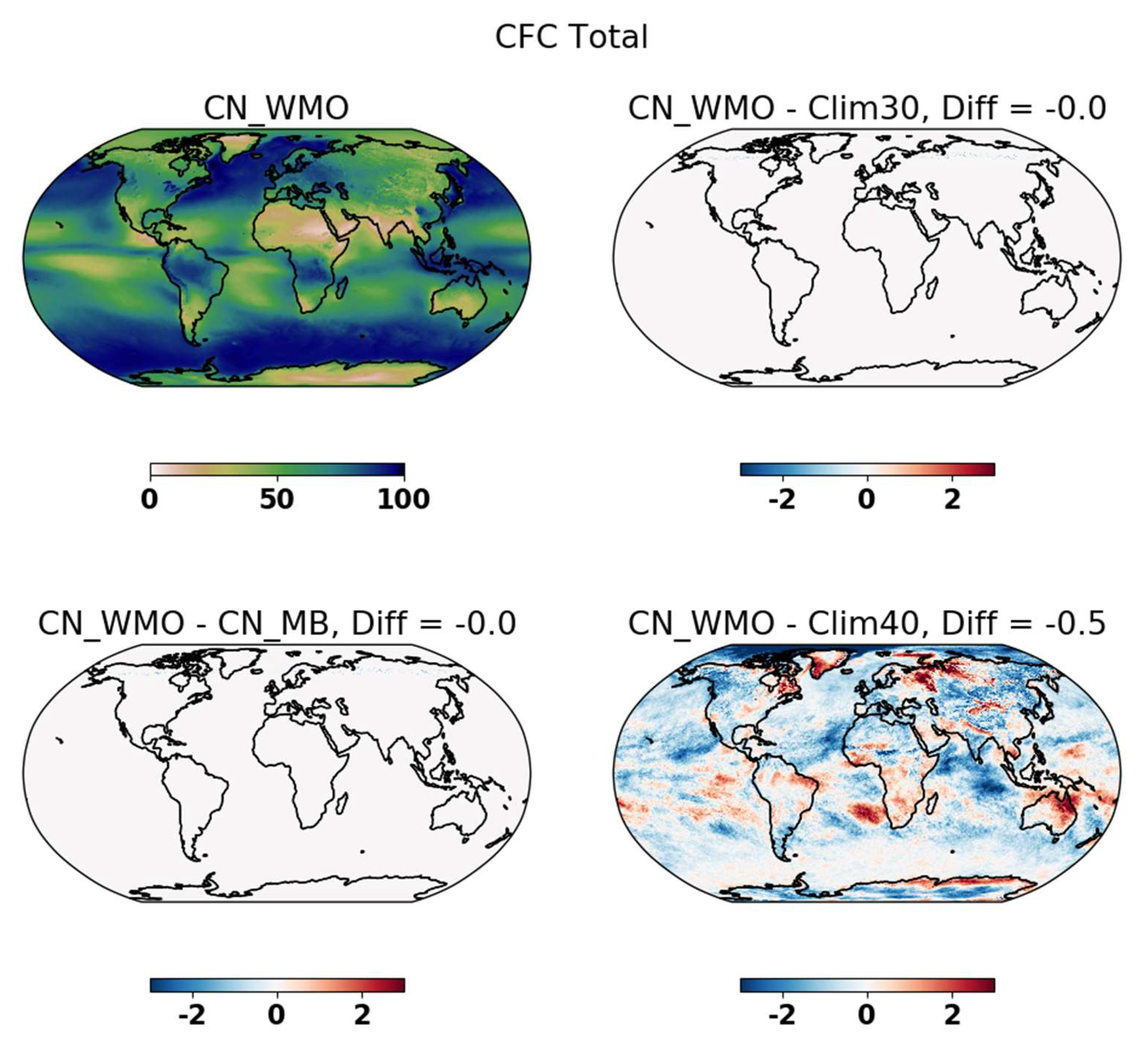
Figure 2.
Latitude-time histograms showing the number of longitude grids failing either the D5 or the D11 condition when computing climate normals of total cloud fraction. Maximum number of longitudes grids can be 1440 since the spatial resolution in 0.25 degrees. The resolution on the Y-axis (latitude) is also 0.25 degrees. .
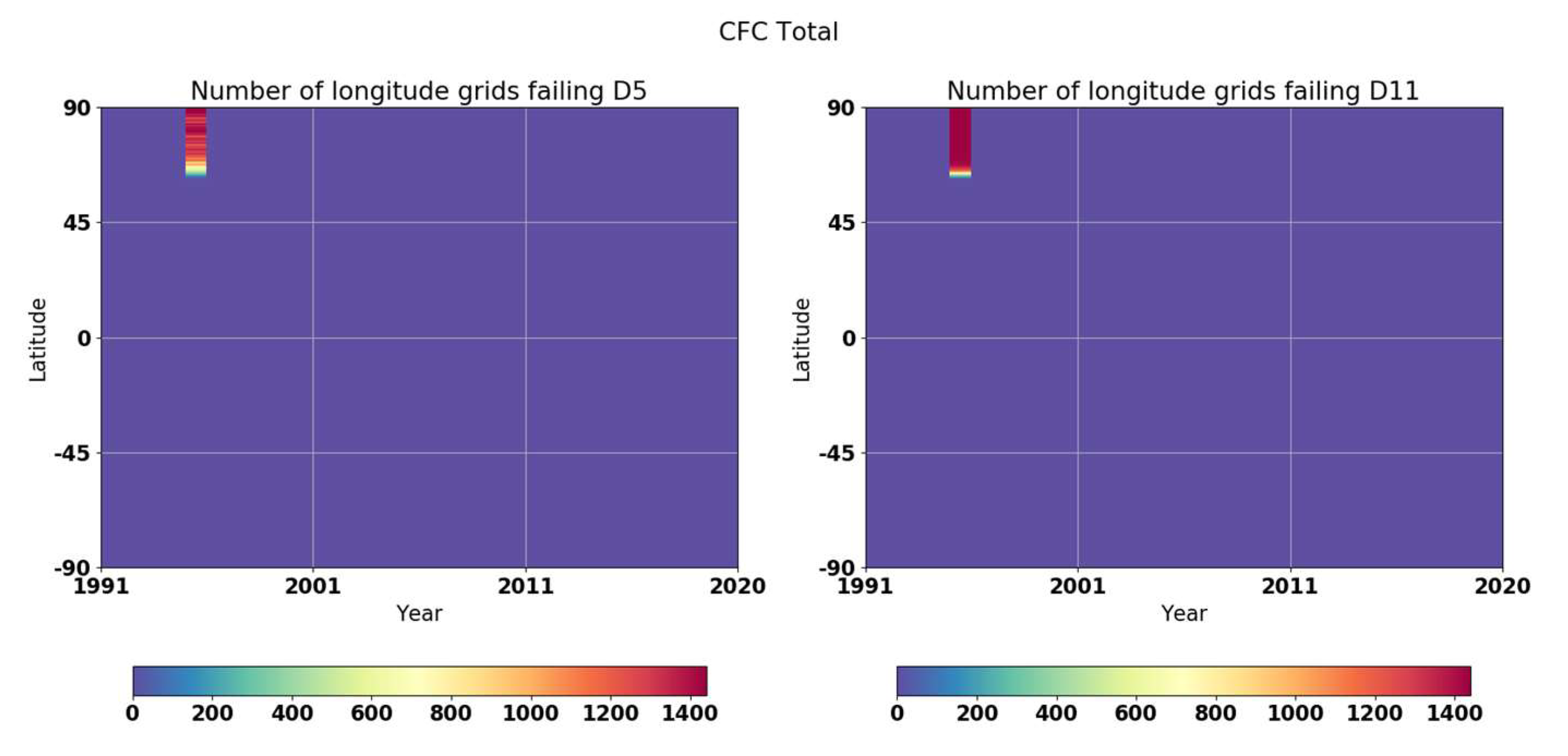
Figure 3.
Same as in Figure 1, but for the low level clouds.
Figure 3.
Same as in Figure 1, but for the low level clouds.
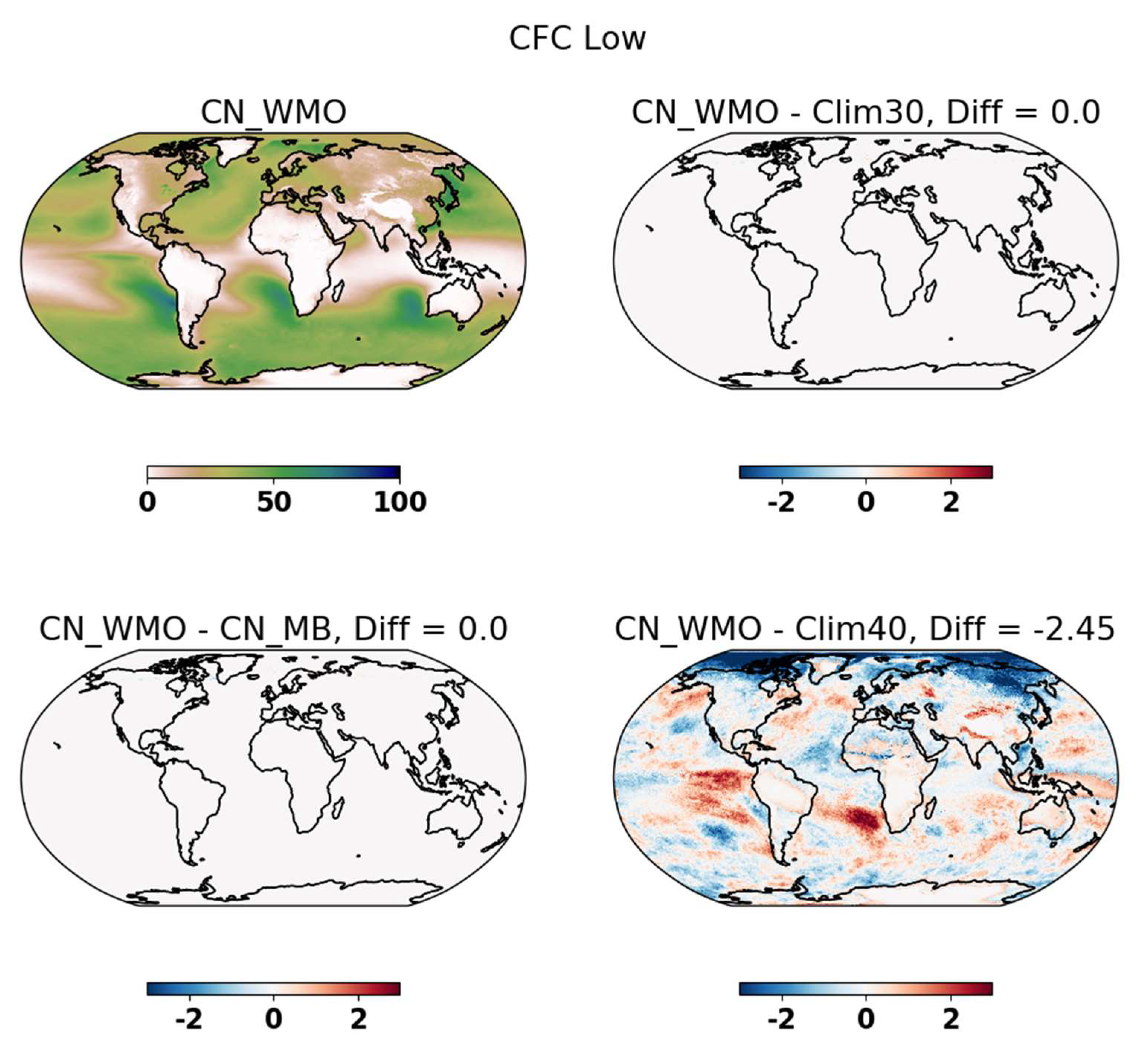
Figure 4.
Same as in Figure 1, but for the daytime cloud fraction.
Figure 4.
Same as in Figure 1, but for the daytime cloud fraction.

Figure 5.
Same as in Figure 1, but for the nighttime cloud fraction.
Figure 5.
Same as in Figure 1, but for the nighttime cloud fraction.
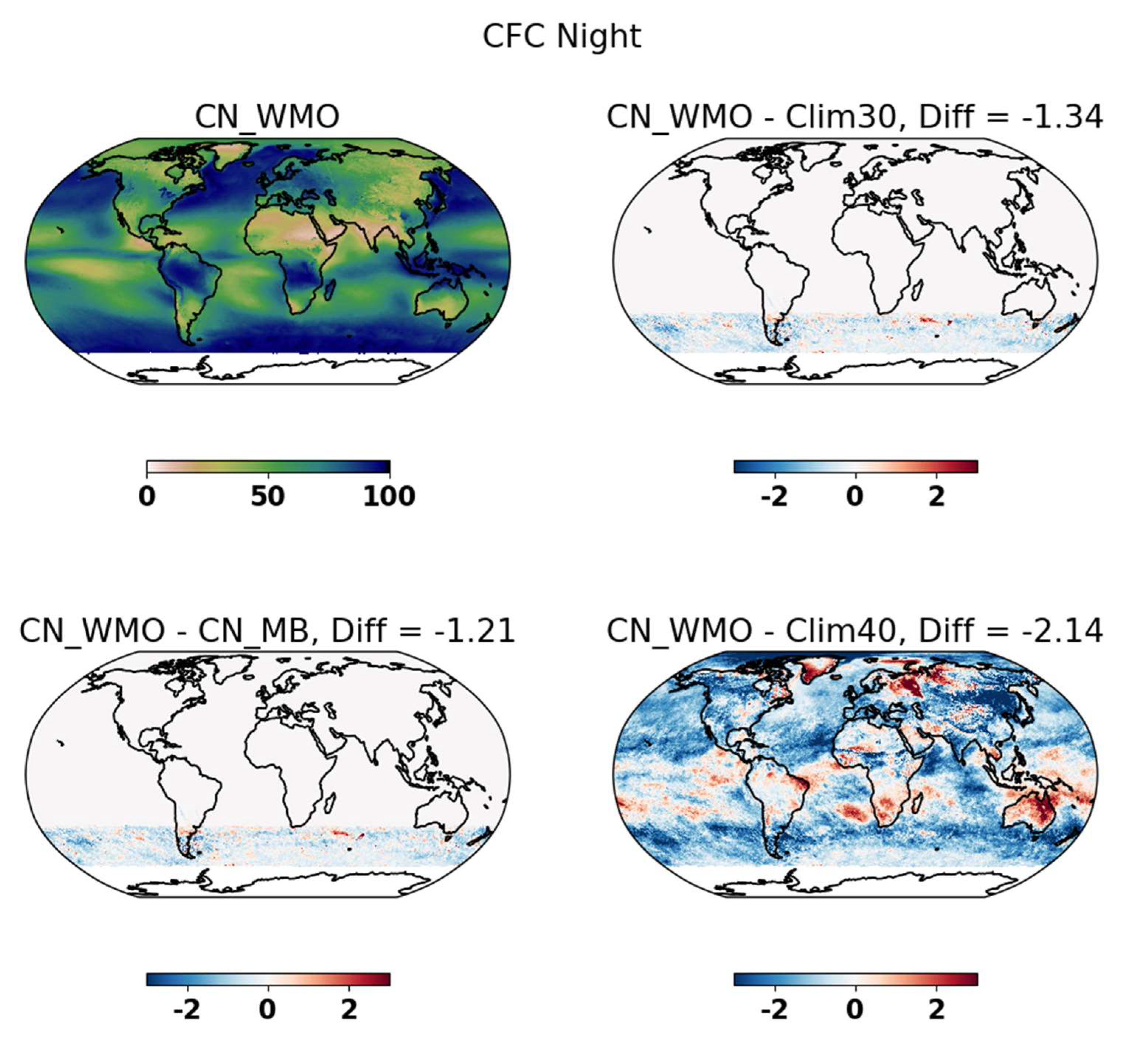
Figure 6.
The number of years, out of total 30, used to compute CN_WMO and Clim30 in the case of daytime cloud fraction and the difference thereof.
Figure 6.
The number of years, out of total 30, used to compute CN_WMO and Clim30 in the case of daytime cloud fraction and the difference thereof.
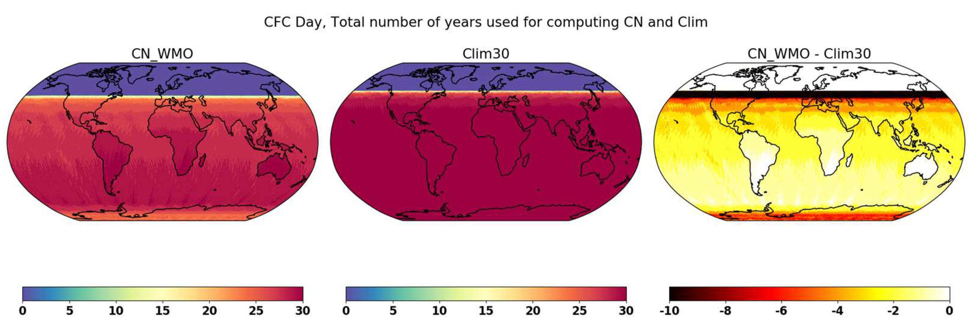
Figure 7.
Latitude-time histograms showing the number of longitude grids failing either the D5 or the D11 condition when computing climate normals of daytime cloud fraction. Maximum number of longitudes grids can be 1400 since the spatial resolution in 0.25 degrees. The resolution on the Y-axis (latitude) is also 0.25 degrees. .
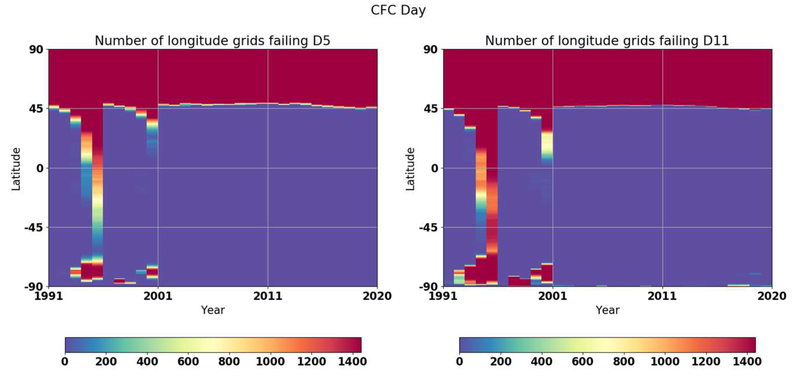
Figure 8.
Same as in Figure 1, but for the cloud top pressure (in hPa).
Figure 8.
Same as in Figure 1, but for the cloud top pressure (in hPa).
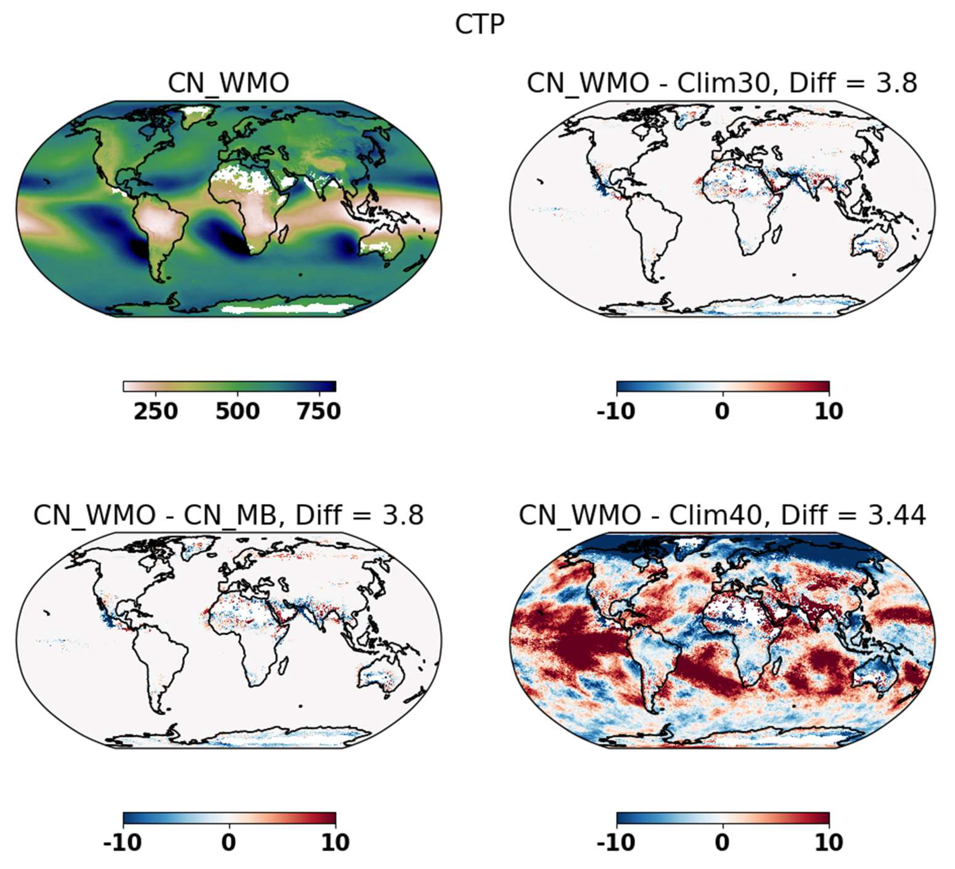
Figure 9.
The number of yearsc, out of total 30, used to compute CN_WMO and Clim30 in the case of cloud top pressure and the difference thereof.
Figure 9.
The number of yearsc, out of total 30, used to compute CN_WMO and Clim30 in the case of cloud top pressure and the difference thereof.
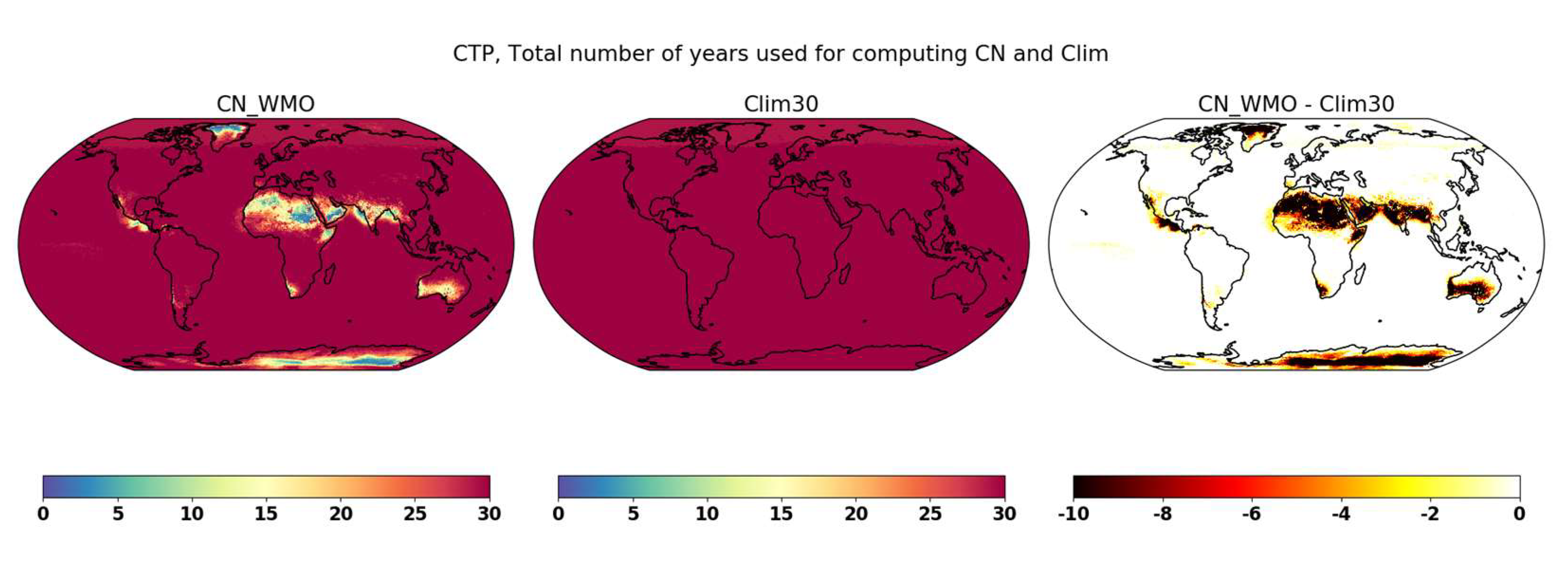
Figure 10.
Latitude-time histograms showing the number of longitude grids failing either the D5 or the D11 condition when computing climate normals of cloud top pressure. Maximum number of longitudes grids can be 1400 since the spatial resolution in 0.25 degrees. The resolution on the Y-axis (latitude) is also 0.25 degrees. .
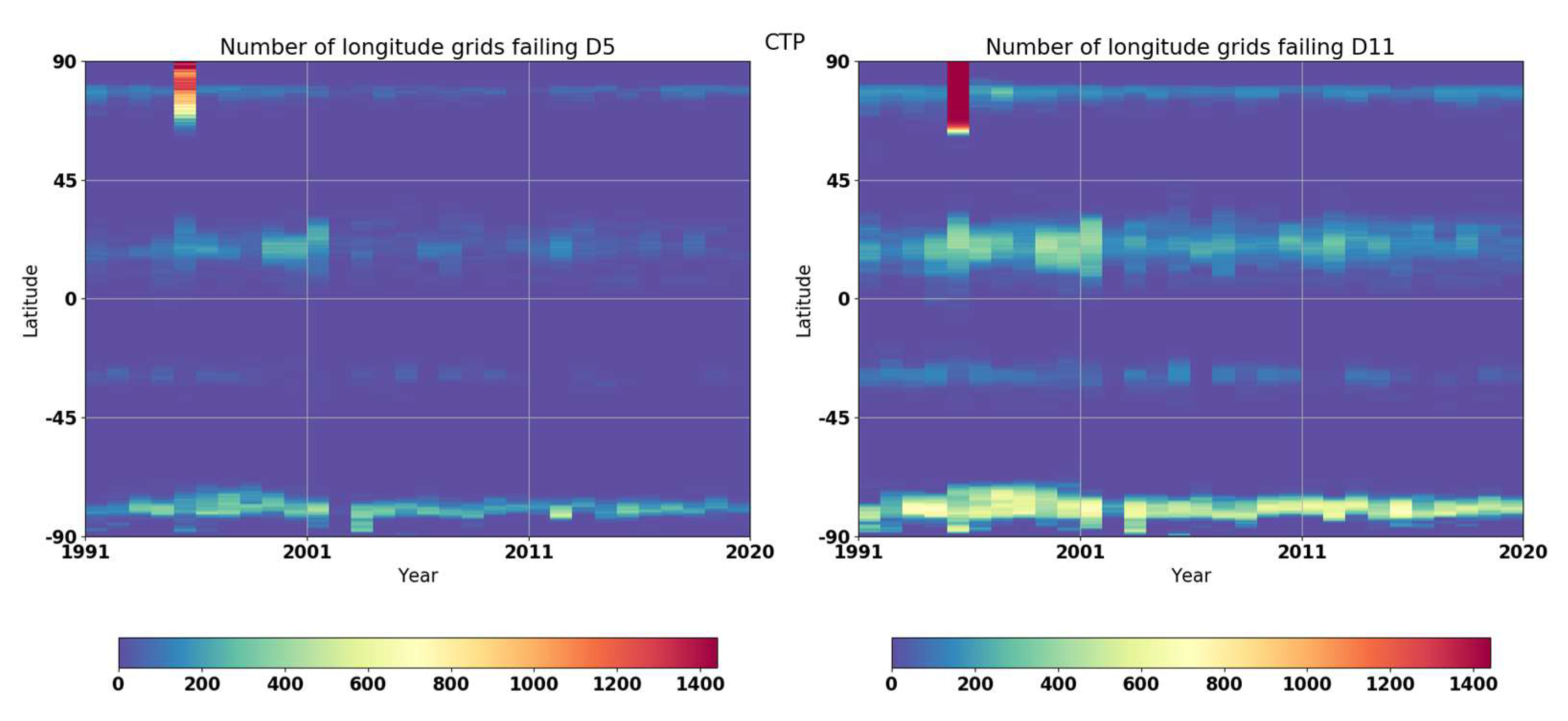
Figure 11.
Same as in Figure 1, but for the incoming solar radiation at the surface (in W/m2).
Figure 11.
Same as in Figure 1, but for the incoming solar radiation at the surface (in W/m2).
Disclaimer/Publisher’s Note: The statements, opinions and data contained in all publications are solely those of the individual author(s) and contributor(s) and not of MDPI and/or the editor(s). MDPI and/or the editor(s) disclaim responsibility for any injury to people or property resulting from any ideas, methods, instructions or products referred to in the content. |
© 2023 by the authors. Licensee MDPI, Basel, Switzerland. This article is an open access article distributed under the terms and conditions of the Creative Commons Attribution (CC BY) license (http://creativecommons.org/licenses/by/4.0/).
Copyright: This open access article is published under a Creative Commons CC BY 4.0 license, which permit the free download, distribution, and reuse, provided that the author and preprint are cited in any reuse.


