Geometrized Vacuum Physics. Part IV: Dynamics of Vacuum Layers

1. Background and Introduction

This paper is the fourth in a series of articles under the general title “Geometrized vacuum physics”. In the previous three articles [1,2,3] the basics of the Algebra of Signatures and the kinematics of vacuum layers were outlined.

Let’s recall that the subject of study of Algebra of Signatures (abbreviated as Alsigna) is the volume of the “vacuum”, i.e., local 3-dimensional area of the void [1,2,3].

Within Alsigna, the “vacuum” is stratified into an infinite number of nested λ_m,n-vacuums, which are illuminated from the void by probing it with monochromatic rays of light with wavelengths λ_m,n from different ranges Δλ =10^m ÷ 10ⁿ cm, where n = m + 1 (see §§1–2 in [1]). In this case, each λ_m,n-vacuum is a 3D_m,n-landscape (or 3D_m,n-lattice), the geodesic lines of which are the corresponding rays of light (see Figure 1).

Figure 1. λ_m,n-vacuum is embedded in λ_f,d-vacuum, where λ_f,d > λ_m,n (repetition of Figure 3 in [3]).

Figure 1. λ_m,n-vacuum is embedded in λ_f,d-vacuum, where λ_f,d > λ_m,n (repetition of Figure 3 in [3]).

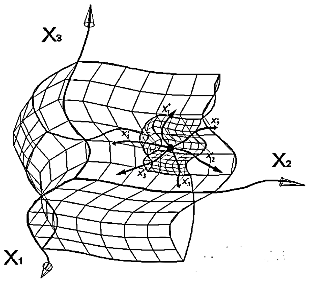
This article considers the geodesic lines of only one curved region of one of the λ_m,n-vacuums. The geodesic lines of the remaining λ_m,n-vacuum are studied similarly.

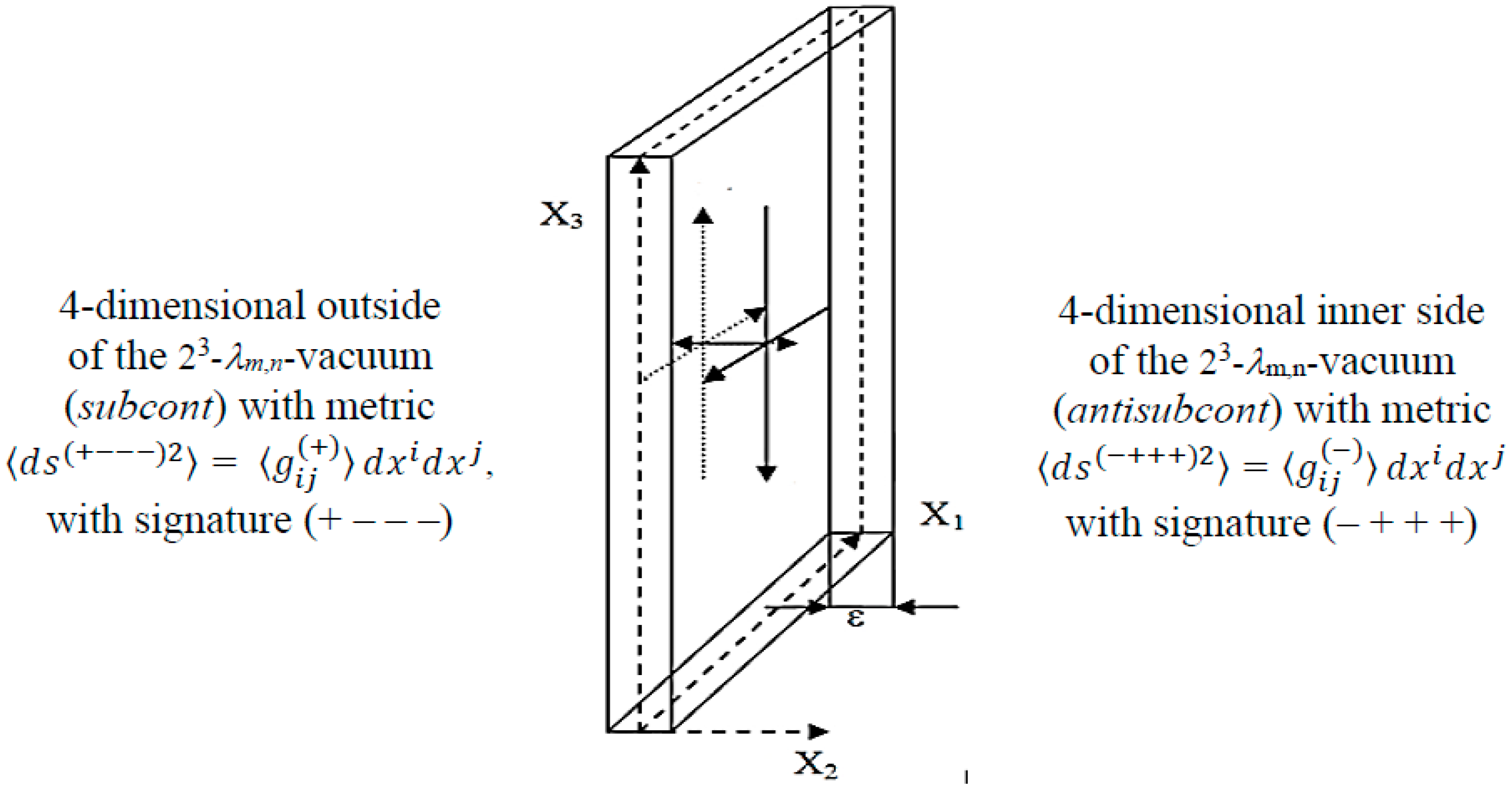
Let’s recall that within the framework of the Algebra of Signature, the simplest level of research is a bilateral consideration of the uncurved local region of the 2³-λ_m,n-vacuum (see §4 in [3] and Figure 2), which is specified by a set of pseudo-Euclidean metrics (83) in [3]

$$\left\{\begin{array}{l}d{s}_0^{\left(+\right)2}=c^{2}d{t}^2-d{x}^2-d{y}^2-d{z}^2=d{s}^{\left(+\right)\prime }d{s}^{\left(+\right)″}=cd{t}^{\prime }cd{t}^{″}-d{x}^{\prime }d{x}^{″}-d{y}^{\prime }d{y}^{″}-d{z}^{\prime }d{z}^{″},\\ d{s}_0^{\left(-\right)2}=-c^{2}d{t}^2+d{x}^2+d{y}^2+d{z}^2=d{s}^{\left(-\right)\prime }d{s}^{\left(-\right)″}=-cd{t}^{\prime }cd{t}^{″}+d{x}^{\prime }d{x}^{″}+d{y}^{\prime }d{y}^{″}+d{z}^{\prime }d{z}^{″}.\end{array}\right.$$

(1)

Figure 2. Simplified illustration of a two-sided section of the 2³-λ_m÷n-vacuum, the outer side of which (subcont) is described by the averaged metric $〈d{s}^{(+---)2}〉$ with the signature (+ – – –), and its inner side (antisubcont) is described by the metric $〈d{s}^{(-+++)2}〉$ with the opposite signature (– + + +), as ε → 0 (repetition of Figure 7 in [3]).

Figure 2. Simplified illustration of a two-sided section of the 2³-λ_m÷n-vacuum, the outer side of which (subcont) is described by the averaged metric $〈d{s}^{(+---)2}〉$ with the signature (+ – – –), and its inner side (antisubcont) is described by the metric $〈d{s}^{(-+++)2}〉$ with the opposite signature (– + + +), as ε → 0 (repetition of Figure 7 in [3]).

The metric-dynamic state of the same, but curved section of the double-sided 2³-λ_m,n-vacuum is described by the averaged metric (61) in [3]

$${\mathit{ds}}^{(\pm )2}=\raisebox{1ex}{$1$}\!\left/ \!\raisebox{-1ex}{$2$}\right.({\mathit{ds}}^{(+---)2}+{\mathit{ds}}^{(-+++)2})=\raisebox{1ex}{$1$}\!\left/ \!\raisebox{-1ex}{$2$}\right.({\mathit{ds}}^{(+)2}+{\mathit{ds}}^{(-)2})=½({g_{\mathit{ij}}}^{(+)}+{g_{\mathit{ij}}}^{(-)}){\mathit{dx}}^i{\mathit{dx}}^j,$$

(2)

where

$${\mathit{ds}}^{(+---)2}={\mathit{ds}}^{(+)2}={g_{\mathit{ij}}}^{(+)}{\mathit{dx}}^i{\mathit{dx}}^j\mathrm{with}\mathrm{signature}(+---),$$

(3)

$$g_{ij}^{(+)}=\left(\begin{array}{cccc}{g}_{00}^{(+)}& g_{10}^{(+)}& g_{20}^{(+)}& g_{30}^{(+)}\\ g_{01}^{(+)}& g_{11}^{(+)}& g_{21}^{(+)}& g_{31}^{(+)}\\ g_{02}^{(+)}& g_{12}^{(+)}& g_{22}^{(+)}& g_{31}^{(+)}\\ g_{03}^{(+)}& g_{13}^{(+)}& g_{23}^{(+)}& g_{33}^{(+)}\end{array}\right)$$

(4)

is metric tensor of the “outer” side of the 2³-λ_m,n-vacuum (i.e., subcont) (see Figure 2);

$${\mathit{ds}}^{(-+++)2}={\mathit{ds}}^{(-)2}={g_{\mathit{ij}}}^{(-)}{\mathit{dx}}^i{\mathit{dx}}^j\mathrm{with}\mathrm{signature}(-+++),$$

(5)

$$g_{ij}^{(-)}=\left(\begin{array}{cccc}{g}_{00}^{(-)}& g_{10}^{(-)}& g_{20}^{(-)}& g_{30}^{(-)}\\ g_{01}^{(-)}& g_{11}^{(-)}& g_{21}^{(-)}& g_{31}^{(-)}\\ g_{02}^{(-)}& g_{12}^{(-)}& g_{22}^{(-)}& g_{31}^{(-)}\\ g_{03}^{(-)}& g_{13}^{(-)}& g_{23}^{(-)}& g_{33}^{(-)}\end{array}\right)$$

(6)

is metric tensor of the “inner” side of the 2³-λ_m,n-vacuum (i.e., antisubcont) (see Figure 2);

Conditional concepts of “subcont” (short for “substantial continuum”) and “antisubcont” (short for “antisubstantial continuum”) were introduced in §7 in [2] to designate, respectively, the outer and inner sides of the 2³-λ_m,n-vacuum, as well as to facilitate the visualization of intertwined intra-vacuum processes. It is conditionally assumed that the “subcont” is formed from streams (threads) of white color, and the antisubcont is formed from streams (threads) of black color (see Figure 3b and Figure 12 in [3]).

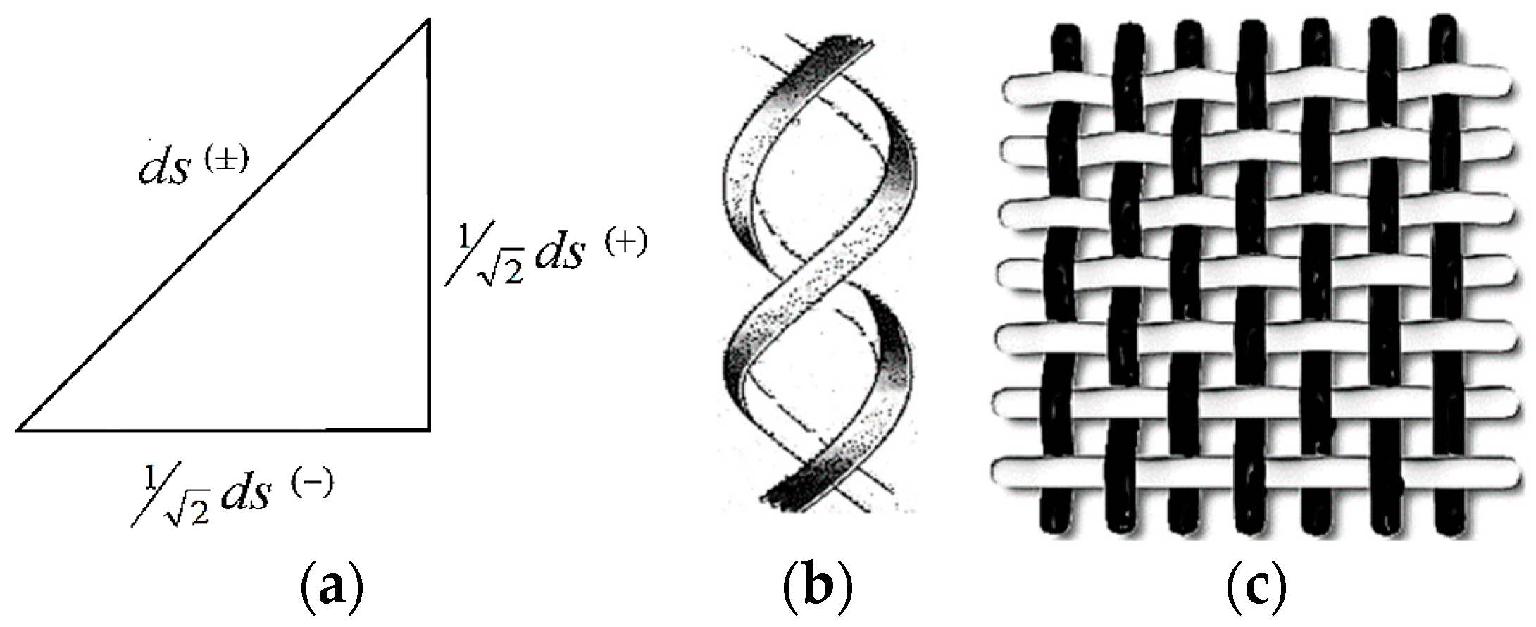
In § 5.2 in [3] it was shown that adjacent segments of the “white” lines ds⁽⁺⁾ of the subcont and the “black” lines ds^(–) of the antisubcont are mutually perpendicular ds⁽⁺⁾ ⊥ ds^(–) (see Figure 3a). This is possible only if they are everywhere intertwined with each other (Figure 3b), and form a 3-dimensional affine fabric of 2³-λ_m,n-vacuum (Figure 3b,c).

Figure 3. a) Mutually perpendicular adjacent segments ($\raisebox{1ex}{$1$}\!\left/ \!\raisebox{-1ex}{$2$}\right.$)^1/2ds⁽⁺⁾ and ($\raisebox{1ex}{$1$}\!\left/ \!\raisebox{-1ex}{$2$}\right.$)^1/2ds^(–); b) If we project a double helix onto a plane, then at the intersection of its lines ds⁽⁺⁾ and ds^(–) are always mutually perpendicular (repetition of Figure 10 in [3]); c) Conventionally, the “white” lines of the ds⁽⁺⁾ subcont and the “black” lines of the ds^(–) antisubcont form a single intertwined affine fabric of the 2³-λ_m,n-vacuum.

Figure 3. a) Mutually perpendicular adjacent segments ($\raisebox{1ex}{$1$}\!\left/ \!\raisebox{-1ex}{$2$}\right.$)^1/2ds⁽⁺⁾ and ($\raisebox{1ex}{$1$}\!\left/ \!\raisebox{-1ex}{$2$}\right.$)^1/2ds^(–); b) If we project a double helix onto a plane, then at the intersection of its lines ds⁽⁺⁾ and ds^(–) are always mutually perpendicular (repetition of Figure 10 in [3]); c) Conventionally, the “white” lines of the ds⁽⁺⁾ subcont and the “black” lines of the ds^(–) antisubcont form a single intertwined affine fabric of the 2³-λ_m,n-vacuum.

Thus, the averaged metric (2) corresponds to a segment of a 2-braid consisting of two mutually intertwined spirals s^(–) and s⁽⁺⁾ (see the definition of a k-braid in § 5.2 in [3]), which can be described by a complex number

$${\mathit{ds}}^{(\pm )}=\frac{1}{\sqrt{2}}({\mathit{ds}}^{(-)}+{\mathit{ids}}^{(+)}),$$

(7)

which we will call a 2-helix. The squared modulus of a complex number (7) (i.e., a 2-helix) is equal to the length of a segment of a 2-braid (2) or expression (61) in [3].

Based on the Algebra of Signature presented in [1,2,3] and partly repeated in this introduction, this article discusses the general dynamics of vacuum layers, from which, under certain conditions, “vacuum electrodynamics” and “vacuum electrostatics” are obtained.

Like the three previous articles [1,2,3], this article is mainly of a theoretical nature and is aimed at further development of the mathematical apparatus of the Algebra of Signature (abbreviated as «Alsigna»).

It is planned that in the following articles of this series, Alsigna’s mathematical apparatus will be used for applied problems, in particular, for the development of a vacuum model of the Universe, a vacuum model of elementary particles, to explain the nature of gravity and electromagnetism, as well as for development of the “zero” (vacuum) technologies.

2. Materials and Method

2.1. Equation of the Geodesic line of a Two-Sided 2³-λ_m,n-Vacuum

The shortest distance between two infinitely close points p₁ and p₂ in a curved area of a two-sided 2³-λ_m,n-vacuum is defined as an extremal of the functional

$$S={\int }_{p1}^{p2}d{s}^{\left(\pm \right)},$$

(8)

where $d{s}^{\left(\pm \right)}$ is a 2-helix (7), integration is performed from point p₁ to point p₂.

We find the equation of this extremal based on the condition that the first variation is equal to zero

$$\delta S={\int }_{p1}^{p2}d{s}^{\left(\pm \right)}=\delta {\int }_{p1}^{p2}\frac{1}{\sqrt{2}}\left(d{s}^{\left(+\right)}+id{s}^{\left(-\right)}\right)=0.$$

(9)

Let’s represent expression (9) in the form

$$\delta S=\frac{1}{\sqrt{2}}\left(\delta {\int }_{p1}^{p2}d{s}^{\left(+\right)}+i\delta {\int }_{p1}^{p2}d{s}^{\left(-\right)}\right)=0,$$

(10)

or taking into account metrics (3) and (5)

$$\delta S=\frac{1}{\sqrt{2}}\left(\sqrt{{g_{ij}}^{(+)}d{x}^{i}d{x}^j}+i\delta {\int }_{p1}^{p2}\sqrt{{g_{ij}}^{(-)}d{x}^{i}d{x}^j}\right)=0.$$

(11)

Expression (11) is equal to zero provided that both terms are equal to zero

$$\delta {\int }_{p1}^{p2}\sqrt{{g_{ij}}^{(+)}d{x}^{i}d{x}^j}=0\mathrm{and}\delta {\int }_{p1}^{p2}\sqrt{{g_{ij}}^{(-)}d{x}^{i}d{x}^j}=0.$$

(12)

In §2 in [3], it was shown that in the most general case, the metric of a local area of a curved 4-dimensional space with any of the 16 possible signatures (22) in [3], can be represented as a scalar product of two vectors given in distorted affine spaces with corresponding stignatures (see Expressions (18)—(20) in [3])

ds^(q)2 = ds^(a)ds^(b) = g_ij^(q)dxⁱdx^j = β^pm(a)e_m^(a)α_pi^(a)β^ln(b)e_n^(b)α_lj^(b)dxⁱdx^j,

(13)

where

ds^(a)=β^pm(a)e_m^(а)α_pi^(a)dxⁱ and ds^(b) = β^ln(b)e_n^(b)α_lj^(b)dx^j

(14)

is vectors defined respectively in the a-th and b-th curved affine space with the corresponding stignature (see §2 in [3]);

α_ij^(a) =dx′^i(a)/dx^j(a)

(15)

is components of the elongation tensor of the axes of the curved region of the a-th affine space with the corresponding stignature from matrix (2) in [2]);

β^pm(a) = (e′_p^(a) ⋅e_m^(a)) = cos (e′_p^{(a) ^}e_m^(a))

(16)

is direction cosines between the axes of the curved section of the a-th affine space with the same stignatura;

• e_m^(a) is basis vector specifying the direction of the m-th axis of the a-th affine space;
• dx^j(a) is an infinitesimal segment of the j-th axis of the a-th affine space.

When parallel translation, for example, a vector ds^(a) (or a vector ds^(b)) in a complexly curved, twisted and displaced affine (i.e., vector) space along a geodesic line from point p₁ to a nearby point p₂ (see Figure 4b), it should be taken into account that the magnitude and direction of this vector may depend on changes in all four parameters α_ij^(a), β^pm(a), e_m^(a), dx^j(a). That is, when translating the vector ds^(a from point p₁ to p₂, in the most complex case the following may change (see Figure 4b): 1) The length of the basis vectors α_ij^(a); 2) angles between the basis vectors β^pm(a); 3) rotation of the entire 4-basis as a whole e_m^(a); 4) Displacement of the 4-basis in general dx^j(a). This is due to the fact that the geodesic line between two points p₁ and p₂ of a complexly distorted space can not only be curved, but also deformed, displaced and twisted.

Figure 4. a) In Riemannian geometry, the parallel translation of the vector ds^(a) from point p₁ to the nearby point p₂ is carried out strictly tangent to the geodesic line connecting these points. In this case, only the direction of this vector changes, and its magnitude remains unchanged. It means that the magnitude of the basis vectors e_m^(а) and the angles between them do not change; b) In the most complexly curved, displaced and twisted space, when transferring (i.e., translation) the vector ds^(a) from point p₁ to the nearby point p₂, its direction, magnitude and displacement may change. When transferring the vector ds^(a) in such a complexly distorted space, the magnitude of the basis vectors e_m^(a) and the angles between them can change, and the 4-basis itself as a whole can rotate and shift. In this case, all four parameters of the 4-basis α_ij^(a), β^pm(a), e_m^(a), dx^j(a) can change, which, according to expression (14), affects the change in the vector ds^(a) when it is transferred.

Figure 4. a) In Riemannian geometry, the parallel translation of the vector ds^(a) from point p₁ to the nearby point p₂ is carried out strictly tangent to the geodesic line connecting these points. In this case, only the direction of this vector changes, and its magnitude remains unchanged. It means that the magnitude of the basis vectors e_m^(а) and the angles between them do not change; b) In the most complexly curved, displaced and twisted space, when transferring (i.e., translation) the vector ds^(a) from point p₁ to the nearby point p₂, its direction, magnitude and displacement may change. When transferring the vector ds^(a) in such a complexly distorted space, the magnitude of the basis vectors e_m^(a) and the angles between them can change, and the 4-basis itself as a whole can rotate and shift. In this case, all four parameters of the 4-basis α_ij^(a), β^pm(a), e_m^(a), dx^j(a) can change, which, according to expression (14), affects the change in the vector ds^(a) when it is transferred.

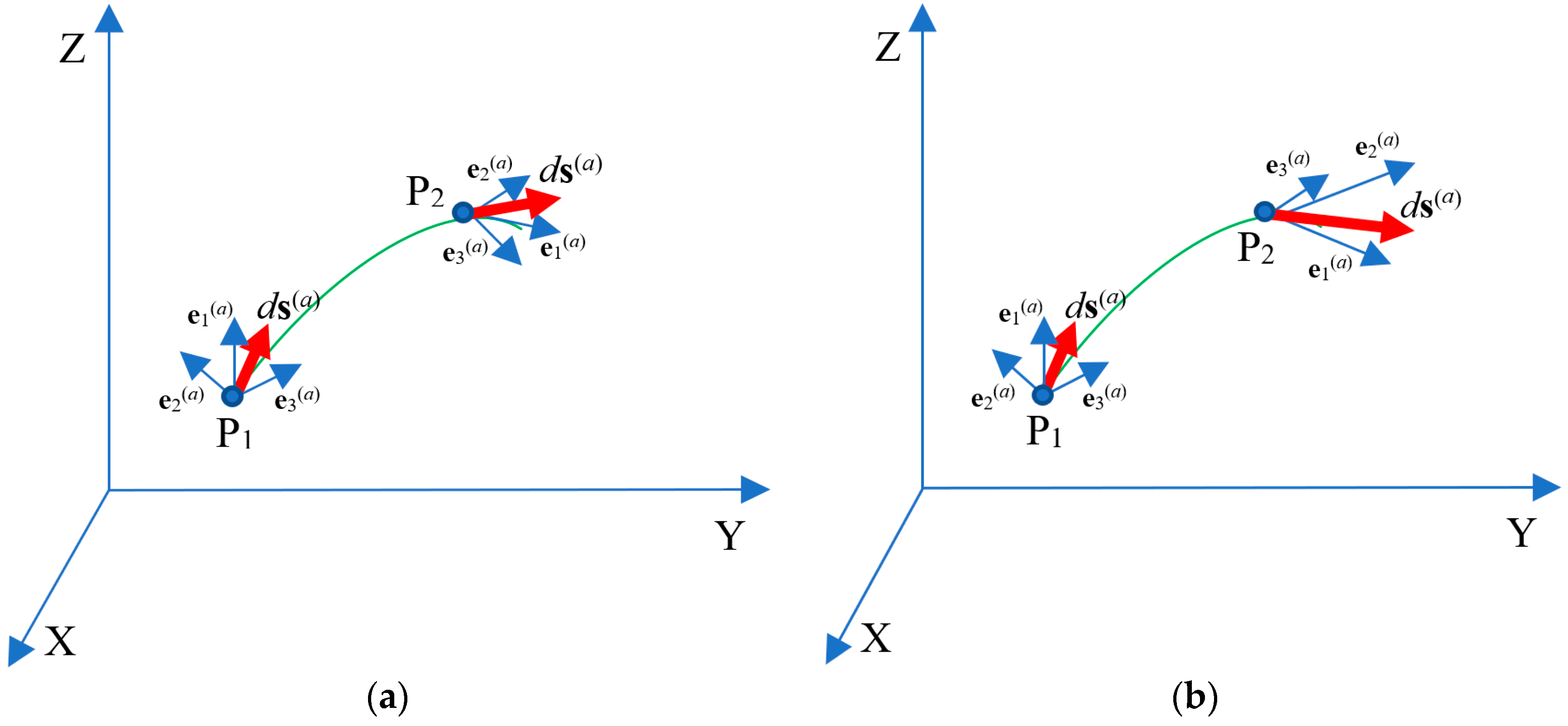
Depending on what distortions, displacements and rotations of the vectors ds^(a) and ds^(b) are taken into account when considering the metric-dynamic properties of curved space, various differential geometries are obtained: for example, Riemannian geometry (see Figure 4a), Weyl geometry, affine geometry of Eddington, geometry with torsion of Cartan-Schouten, geometry of absolute parallelism of Weizenbeck-Vitali-Shipov [4], etc.

2.2. Equation of the Geodesic Line of a Two-Sided 2³-λ_m,n-Vacuum in the Case of Riemannian Geometry

First, let’s assume that the outer and inner 4-dimensional sides of the 2³-λ_m,n-vacuum (i.e., subcont and antisubcont) are only curved, i.e., are described by the simplest differential Riemannian geometry (see Figure 4a). In this case, the extremals of functionals (12) are defined identically, so we introduce a generalized metric

$$d{s}^2=g_{ij}d{x}^{i}d{x}^j\leftrightarrow \left\{\begin{array}{c}ord{s}^{(+)2}=g_{ij}^{(+)}d{x}^{i}d{x}^j,\\ ord{s}^{(-)2}=g_{ij}^{(-)}d{x}^{i}d{x}^j.\end{array}\right.$$

We consider the general case

$$\delta {\int }_{p1}^{p2}ds=\delta {\int }_{p1}^{p2}\sqrt{g_{ij}d{x}^{i}d{x}^j}=0,$$

(17)

provided that at the ends of the desired geodesic line ds (i.e., at points p₁ and p₂) the variations are zero

$$\delta d{s}_{\left({\mathrm{p}}_1\right)}=\delta d{s}_{\left({\mathrm{p}}_2\right)}=\delta x_{\left({\mathrm{p}}_1\right)}=\delta x_{\left({\mathrm{p}}_2\right)}=0.$$

(18)

Let’s use the expression

$$\delta d{s}^2=2ds\delta ds,$$

(19)

whence it follows [5]

$$\delta ds=\frac{1}{2ds}\delta g_{ij}d{x}^{i}d{x}^j=\frac{1}{2ds}\left[\frac{\partial g_{ij}}{\partial x^{\mu }}\delta x^{\mu }d{x}^{i}d{x}^j+g_{ij}d{x}^{j}d\delta x^i+g_{ij}d{x}^{i}d\delta x^j\right],$$

(20)

where the commutativity of the operations of variation and differentiation $\delta \left(d{x}^i\right)=d\left(\delta x^i\right)$ is used.

Let’s substitute Ex. (20) under the integral (17), and divide and multiply this expression by ds, as a result we obtain [5]

$$\delta S=\frac{1}{2}{\int }_{{\mathrm{p}}_1}^{{\mathrm{p}}_2}\left\{\frac{\partial g_{ij}}{\partial x^{\mu }}\frac{d{x}^i}{ds}\frac{d{x}^j}{ds}\delta x^{\mu }+\left(g_{\mu j}\frac{d{x}^j}{ds}+g_{i\mu }\frac{d{x}^i}{ds}\right)\frac{d\left(\delta x^{\mu }\right)}{ds}\right\}ds=0.$$

(21)

We integrate the expression in parentheses by parts [5]:

$$\frac{1}{2}{\int }_{{\mathrm{p}}_1}^{{\mathrm{p}}_2}\left(g_{\mu j}\frac{d{x}^j}{ds}+g_{i\mu }\frac{d{x}^i}{ds}\right)\frac{d\left(\delta x^{\mu }\right)}{ds}ds={\left.\frac{1}{2}\left(g_{\mu k}\frac{d{x}^k}{ds}+g_{i\mu }\frac{d{x}^i}{ds}\right)\delta x^{\mu }\right|}_{{\mathrm{p}}_1}^{{\mathrm{p}}_2}-\frac{1}{2}{\int }_{{\mathrm{p}}_1}^{{\mathrm{p}}_2}\delta x^{\mu }\frac{d}{ds}\left(g_{\mu j}\frac{d{x}^j}{ds}+g_{i\mu }\frac{d{x}^i}{ds}\right)ds.$$

(22)

The first term in this expression, due to conditions (18), becomes zero. Let’s substitute the remaining part of expression (22) into equation (21) and perform differentiation, as a result we obtain [5]:

$$\delta S=\frac{1}{2}{\int }_{{\mathrm{p}}_1}^{{\mathrm{p}}_2}\left\{\left(\frac{\partial g_{ij}}{\partial x^{\mu }}-\frac{\partial g_{\mu j}}{\partial x^i}-\frac{\partial g_{i\mu }}{\partial x^j}\right)\frac{d{x}^i}{ds}\frac{d{x}^j}{ds}+2g_{\mu j}\frac{d^2{x}^j}{d{s}^2}\right\}ds\delta x^{\mu }=0.$$

(23)

From the fact that integral (23) vanishes for any variations of δх^μ, it follows that the expression enclosed in curly brackets is equal to zero. From where, taking into account the relation $g_{ij}{g}^{ij}=4$, after simple calculations we obtain the equation of the geodesic line [5]:

$$\frac{d^2{x}^l}{d{s}^2}+{Г}_{ij}^l\frac{d{x}^i}{ds}\frac{d{x}^j}{ds}=0,$$

(24)

where

$${Г}_{ij}^l=\frac{1}{2}{g}^{l\mu }\left(\frac{\partial g_{\mu i}}{\partial x^j}+\frac{\partial g_{\mu j}}{\partial x^i}-\frac{\partial g_{ij}}{\partial x^{\mu }}\right)\mathrm{is}\mathrm{Christoffel}\mathrm{symbols};$$

(25)

$x^i$(s) is coordinates of the curved line.

Equation (24) is intended to determine the extremal of functional (17) with simplifications related to Riemannian geometry (Figure 4a). This equation determines the most optimal (geodesic) line connecting two close points p₁ and p₂ in a curved 4-dimensional space. That is, this is a line that, under the above conditions, allows you to get from point p₁ to the nearby point p₂ in the shortest time and with the least energy costs.

At the same time, Equation (24) can be represented in the form

$$\frac{d^2{x}^l}{d{s}^2}=-{Г}_{ij}^l\frac{d{x}^i}{ds}\frac{d{x}^j}{ds},$$

(26)

this equation defines the 4-acceleration field $d^2{x}^l/d{s}^2$, which can be interpreted as a massless force field$f^l$

$$\frac{d^2{x}^l}{d{s}^2}=f^l/m_b,$$

where $m_b$ is the mass of a body that is carried away by a continuous “medium”, which moving with acceleration $d^2{x}^l/d{s}^2$.

At this stage of research, it is difficult to explain what is meant by a force field in vacuum physics. However, it is possible to compare the acceleration of a local section of the vacuum layer with the accelerated movement of a small volume of liquid in the general flow of the river. Such an accelerated flow carries with it everything that comes in its way and makes it move with the same acceleration. From the point of view of post-Newtonian physics, if a body moves with acceleration, then a force acts on it. Therefore, the accelerated movement of the local volume of a 3-dimensional medium (in this case, subcont, or antisubcont) can be interpreted as a local force effect.

Performing separately similar operations (17) – (24) for variations (12), we obtain two equations

$$\frac{d^2{x}^l}{d{s}^2}+{Г}_{ij}^{l(-)}\frac{d{x}^i}{ds}\frac{d{x}^j}{ds}=0,$$

(27)

$$\frac{d^2{x}^l}{d{s}^2}+{Г}_{ij}^{l(+)}\frac{d{x}^i}{ds}\frac{d{x}^j}{ds}=0,$$

(28)

where respectively

$${Г}_{ij}^{l(+)}=\frac{1}{2}{g}^{l\mu (+)}\left(\frac{\partial g_{\mu i}^{(+)}}{\partial x^j}+\frac{\partial g_{\mu j}^{(+)}}{\partial x^i}-\frac{\partial g_{ij}^{(+)}}{\partial x^{\mu }}\right)$$

(29)

is Christoffel symbols of a subcont;

$${Г}_{ij}^{l(-)}=\frac{1}{2}{g}^{l\mu (-)}\left(\frac{\partial g_{\mu i}^{(-)}}{\partial x^j}+\frac{\partial g_{\mu j}^{(-)}}{\partial x^i}-\frac{\partial g_{ij}^{(-)}}{\partial x^{\mu }}\right)$$

(30)

is Christoffel symbols of a antisubcont;

When considering variation (11), taking into account the Christoffel symbols (29) and (30), we find that the sought-for extremal of the functional (8), with simplifications related to Riemannian geometry, is determined by the following equation of a geodesic line in a curved two-sided 2³-λ_m,n-vacuum

$$\frac{d^2{x}^l}{d{s}^2}+\frac{1}{\sqrt{2}}({Г}_{ij}^{l(+)}+i{Г}_{ij}^{l(-)})\frac{d{x}^i}{ds}\frac{d{x}^j}{ds}=0,$$

(31)

or

$$\frac{d^2{x}^l}{d{s}^2}=-\frac{1}{\sqrt{2}}\left({Г}_{ij}^{l\left(+\right)}+i{Г}_{ij}^{l\left(-\right)}\right)\frac{d{x}^i}{ds}\frac{d{x}^j}{ds}.$$

(32)

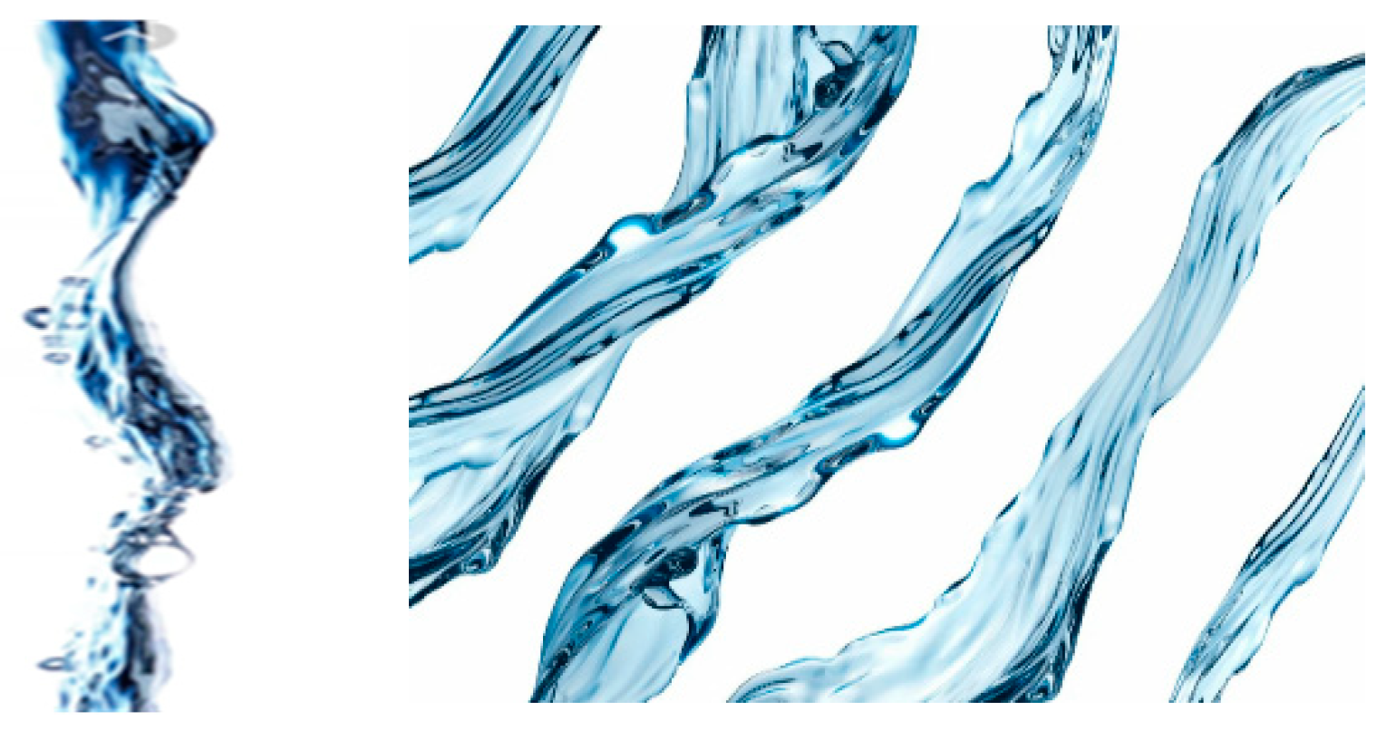
Ex. (31) shows that the geodesic lines of the subcont and antisubcont, i.e., two mutually opposite sides of the local section of the two-sided 2³-λ_m,n-vacuum is twisted into a 2-spiral. This is similar to how rivulets twist in a freely falling jet of liquid (see Figure 5).

Figure 5. Many streams in a freely falling stream of liquid twist into a spiral.

Figure 5. Many streams in a freely falling stream of liquid twist into a spiral.

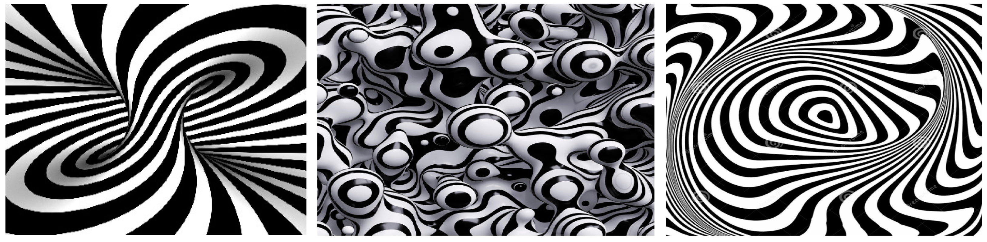
Continuing the analogy with liquid, it should be noted that within the framework of the Algebra of Signature, a two-sided 2³-λ_m,n-vacuum can be represented as an interweaving (mixing) of two liquids (subcont and antisubcomt), which can be conditionally “colored” in white and black colors (see Figure 6). These two conjugate “liquids” cannot separately move in a straight line; they are interconnected and can move in one direction only by twisting into a 2-helix.

Figure 6. Illustrations of mixing of white and black “liquids”.

Figure 6. Illustrations of mixing of white and black “liquids”.

2.3. Equation of the Geodesic Line of a 16-sided 2⁶-λ_m,n-Vacuum in the Case of Riemannian Geometry

In the previous paragraph, we considered the most simplified model representation of the interweaving of geodesic lines of a two-sided 2³-λ_m,n-vacuum which can be interpreted as mixing and interweaving of flows of two liquids: conventionally “white” and “black”). With a more detailed examination of such conjugate “multi-colored” liquids there should be 16. With an even more detailed examination of these liquids there are already 256 and so on ad infinitum.

More in-depth and accurate is the sixteen-sided consideration of the local area of the 2⁶-λ_m,n-vacuum (see §3 and §5.3 in [3]). In this case, the curved state of the 2⁶-λ_m,n-vacuum is described by a superposition (averaging) not of two, as in the previous paragraph, but of sixteen 4-metrics (see Ex. (25) in [3]).

$$\begin{gathered} s_{\left(16\right)}^2=\frac{1}{16}{\sum }_{q=1}^{16}{g}_{ij}^{\left(q\right)}d{x}_{i}d{x}_j=\frac{1}{16}\left[g_{ij}^{\left(1\right)}d{x}^{i}d{x}^j+g_{ij}^{\left(2\right)}d{x}^{i}d{x}^j+g_{ij}^{\left(3\right)}d{x}^{i}d{x}^j+g_{ij}^{\left(4\right)}d{x}^{i}d{x}^j\right.+ \\ +g_{ij}^{\left(5\right)}d{x}^{i}d{x}^j+g_{ij}^{\left(6\right)}d{x}^{i}d{x}^j+g_{ij}^{\left(7\right)}d{x}^{i}d{x}^j+g_{ij}^{\left(8\right)}d{x}^{i}d{x}^j+ \\ +g_{ij}^{\left(9\right)}d{x}^{i}d{x}^j+g_{ij}^{\left(10\right)}d{x}^{i}d{x}^j+g_{ij}^{\left(11\right)}d{x}^{i}d{x}^j+g_{ij}^{\left(12\right)}d{x}^{i}d{x}^j+ \\ \left.+g_{ij}^{\left(13\right)}d{x}^{i}d{x}^j+g_{ij}^{\left(14\right)}d{x}^{i}d{x}^j+g_{ij}^{\left(15\right)}d{x}^{i}d{x}^j+g_{ij}^{\left(16\right)}d{x}^{i}d{x}^j\right]=0, \end{gathered}$$

(33)

where

$$g_{ij}^{\left(q\right)}=\left(\begin{array}{cccc}{g}_{00}^{\left(q\right)}& g_{10}^{\left(q\right)}& g_{20}^{\left(q\right)}& g_{30}^{\left(q\right)}\\ g_{01}^{\left(q\right)}& g_{11}^{\left(q\right)}& g_{21}^{\left(q\right)}& g_{31}^{\left(q\right)}\\ g_{02}^{\left(q\right)}& g_{12}^{\left(q\right)}& g_{22}^{\left(q\right)}& g_{32}^{\left(q\right)}\\ g_{03}^{\left(q\right)}& g_{13}^{\left(q\right)}& g_{23}^{\left(\mathrm{p}\right)}& g_{33}^{\left(q\right)}\end{array}\right)$$

(34)

is components of the metric tensor of the q-th metric space with a signature from the matrix (22) in [3]:

$$sign\left(g_{ij}^{\left(q\right)}\right)=\begin{array}{cccc}{\left(++++\right)}^1& {\left(+++-\right)}^5& {\left(-++-\right)}^9& {\left(++-+\right)}^{13}\\ {\left(---+\right)}^2& {\left(-+++\right)}^6& {\left(--++\right)}^{10}& {\left(-+-+\right)}^{14}\\ {\left(+--+\right)}^3& {\left(++--\right)}^7& {\left(+---\right)}^{11}& {\left(+-++\right)}^{15}\\ {\left(--+-\right)}^4& {\left(+-+-\right)}^8& {\left(-+--\right)}^{12}& {\left(----\right)}^{16}.\end{array}$$

(35)

In the framework of the Algebra of Signature, Ex. (33) is called a 16-braid, which is formed by the additive superposition of sixteen 4-dimensional metric spaces (see §5.3 in [3]). In this case, a section of a 16-braid is formed from sixteen intertwined “colored” lines (spiral threads) ds^(q), and is described by Ex. (69) in [3]

ds⁽¹⁶⁾ = 1√16 (η₁ ds^{(+– – –)} + η₂ ds^{(+ + + +)} + η₃ ds^{(– – – +)} + η₄ ds^{(+ – – +)} +
+ η₅ ds^{(– – + –)} + η₆ ds^{(+ + – –)} + η₇ ds^{(– + – –)} + η₈ ds^{(+ – + –)} +
+ η₉ ds^{(– + + +)} + η₁₀ ds^{(– – – –)} + η₁₁ ds^{(+ + + –)} + η₁₂ ds ^{(– + + –)} +
+ η₁₃ ds^{(+ + – +)} + η₁₄ ds^{(– – + +)} + η₁₅ ds^{(+ – + +)} + η₁₆ ds^{(– + – +)}),

(36)

where η_m (m = 1,2,3,…,16) is an orthonormal basis of objects (similar to the imaginary unit i) satisfying the anticommutative Clifford algebra relation (68) in [3]

η_mη_n + η_nη_m = 2δ_mn ,

(37)

where δ_nm is the unit 16×16 matrix.

For example, let‘s imagine a segment of a 16-helix (36) as a sum of two complex conjugated 8-helices (octonions) with signatures {+ – – –} and {– + + +}

$${\mathit{ds}}_{\left(16\right)}=1/\sqrt{2}({{\mathit{ds}}_{\left(8\right)}}^{(+)}+{{\mathit{ids}}_{\left(8\right)}}^{(-)}),$$

(38)

where

ds⁽⁸⁾⁽⁺⁾ = 1/√8 (ζ₁ds^{(+ + + +)} + ζ₂ds^{(+ – – –)} + ζ₃ds^{(– – – +)} + ζ₄ds^{(+ – – +)} + ζ₅ds^{(– – + –)} + ζ₆ ds^{(+ + – –)} + ζ₇ds ^{(– + – –)} + ζ₈ds^{(+ – + –)})

(39)

,

ds^(8)(–) = 1/√8 (ζ₁ds^{(– – – – )} + ζ₂ds^{(– + + +)} + ζ₃ds^{(+ + + –)} + ζ₄ds^{(– + + –)} + ζ₅ ds^{(+ + – +)} + ζ₆ ds^{(– – + +)} + ζ₇ ds^{(+ – + +)} + ζ₈ ds^{(– + – +)}),

(40)

where the objects ζ_r (where r = 1, 2, 3, … ,8), as well as the objects ηm, satisfy the anticommutative relations of the Clifford algebra:

ζ_m ζ_k + ζ_k ζ_m = 2δ_km ,

(41)

where δ_km is the Kronecker symbol (δ_km = 0 for m ≠ k and δ_km = 1 for m = k).

These requirements are satisfied, for example, by a set of 8×8 matrices of type (65) in [1]:

$$\begin{gathered} {\zeta }_1=\left(\begin{array}{cccccccc}1& 0& 0& 0& 0& 0& 0& 0\\ 0& 1& 0& 0& 0& 0& 0& 0\\ 0& 0& 1& 0& 0& 0& 0& 0\\ 0& 0& 0& 1& 0& 0& 0& 0\\ 0& 0& 0& 0& 1& 0& 0& 0\\ 0& 0& 0& 0& 0& 1& 0& 0\\ 0& 0& 0& 0& 0& 0& 1& 0\\ 0& 0& 0& 0& 0& 0& 0& 1\end{array}\right){\zeta }_2=\left(\begin{array}{cccccccc}0& 1& 0& 0& 0& 0& 0& 0\\ -1& 0& 0& 0& 0& 0& 0& 0\\ 0& 0& 0& -1& 0& 0& 0& 0\\ 0& 0& 1& 0& 0& 0& 0& 0\\ 0& 0& 0& 0& 0& -1& 0& 0\\ 0& 0& 0& 0& 1& 0& 0& 0\\ 0& 0& 0& 0& 0& 0& 0& 1\\ 0& 0& 0& 0& 0& 0& -1& 0\end{array}\right) \\ {\zeta }_3=\left(\begin{array}{cccccccc}0& 0& 1& 0& 0& 0& 0& 0\\ 0& 0& 0& 1& 0& 0& 0& 0\\ -1& 0& 0& 0& 0& 0& 0& 0\\ 0& -1& 0& 0& 0& 0& 0& 0\\ 0& 0& 0& 0& 0& 0& -1& 0\\ 0& 0& 0& 0& 0& 0& 0& -1\\ 0& 0& 0& 0& 0& 1& 0& 0\\ 0& 0& 0& 0& 0& 0& 1& 0\end{array}\right){\zeta }_4=\left(\begin{array}{cccccccc}0& 0& 0& 1& 0& 0& 0& 0\\ 0& 0& -1& 0& 0& 0& 0& 0\\ 0& 1& 0& 0& 0& 0& 0& 0\\ -1& 0& 0& 0& 0& 0& 0& 0\\ 0& 0& 0& 0& 0& 0& 0& -1\\ 0& 0& 0& 0& 0& 0& 1& 0\\ 0& 0& 0& 0& 0& -1& 0& 0\\ 0& 0& 0& 0& 1& 0& 0& 0\end{array}\right) \\ {\zeta }_5=\left(\begin{array}{cccccccc}0& 0& 0& 0& 1& 0& 0& 0\\ 0& 0& 0& 0& 0& 1& 0& 0\\ 0& 0& 0& 0& 0& 0& 1& 0\\ 0& 0& 0& 0& 0& 0& 0& 1\\ -1& 0& 0& 0& 0& 0& 0& 0\\ 0& -1& 0& 0& 0& 0& 0& 0\\ 0& 0& -1& 0& 0& 0& 0& 0\\ 0& 0& 0& -1& 0& 0& 0& 0\end{array}\right){\zeta }_6=\left(\begin{array}{cccccccc}0& 0& 0& 0& 0& 1& 0& 0\\ 0& 0& 0& 0& -1& 0& 0& 0\\ 0& 0& 0& 0& 0& 0& 0& 1\\ 0& 0& 0& 0& 0& 0& -1& 0\\ 0& 1& 0& 0& 0& 0& 0& 0\\ -1& 0& 0& 0& 0& 0& 0& 0\\ 0& 0& 0& 1& 0& 0& 0& 0\\ 0& 0& -1& 0& 0& 0& 0& 0\end{array}\right) \\ {\zeta }_7=\left(\begin{array}{cccccccc}0& 0& 0& 0& 0& 0& 1& 0\\ 0& 0& 0& 0& 0& 0& 0& -1\\ 0& 0& 0& 0& -1& 0& 0& 0\\ 0& 0& 0& 0& 0& 1& 0& 0\\ 0& 0& 1& 0& 0& 0& 0& 0\\ 0& 0& 0& -1& 0& 0& 0& 0\\ -1& 0& 0& 0& 0& 0& 0& 0\\ 0& 1& 0& 0& 0& 0& 0& 0\end{array}\right){\zeta }_8=\left(\begin{array}{cccccccc}0& 0& 0& 0& 0& 0& 0& 1\\ 0& 0& 0& 0& 0& 0& 1& 0\\ 0& 0& 0& 0& 0& -1& 0& 0\\ 0& 0& 0& 0& -1& 0& 0& 0\\ 0& 0& 0& 1& 0& 0& 0& 0\\ 0& 0& 1& 0& 0& 0& 0& 0\\ 0& -1& 0& 0& 0& 0& 0& 0\\ -1& 0& 0& 0& 0& 0& 0& 0\end{array}\right) \end{gathered}$$

(42)

In this case, δ_km is a unit 8×8-matrix:

$${\delta }_{km}=\left(\begin{array}{cccccccc}1& 0& 0& 0& 0& 0& 0& 0\\ 0& 1& 0& 0& 0& 0& 0& 0\\ 0& 0& 1& 0& 0& 0& 0& 0\\ 0& 0& 0& 1& 0& 0& 0& 0\\ 0& 0& 0& 0& 1& 0& 0& 0\\ 0& 0& 0& 0& 0& 1& 0& 0\\ 0& 0& 0& 0& 0& 0& 1& 0\\ 0& 0& 0& 0& 0& 0& 0& 1\end{array}\right)$$

(43)

Similarly, the objects η_m can be represented by sixteen 16x16 matrices.

Let’s look at the functional

$$S={\int }_{{\mathrm{p}}_1}^{{\mathrm{p}}_2}d{s}_{\left(16\right)},$$

(44)

where ds⁽¹⁶⁾ is a segment of the 16-helix (36).

Let’s equate the first variation of this functional to zero

^δS = 1/√16 (η₁δ ∫ ds^{(+ – – –)} + η₂δ ∫ ds^{(+ + + +)} + η₃δ ∫ ds^{(– – – +)} + η₄δ ∫ ds^{(+ – – +)} +
+ η₅δ ∫ ds^{(– – + –)} + η₆ δ ∫ ds^{(+ + – –)} + η₇ δ ∫ ds^{(– + – –)} + η₈δ ∫ ds^{(+ – + –)} +
+ η₉δ ∫ ds^{(– + + +)} + η₁₀δ ∫ds^{(– – – –)} + η₁₁δ ∫ ds^{(+ + + –)} + η₁₂δ ∫ds ^{(– + + –)} +
+ η₁₃δ ∫ ds^{(+ + – +)} + η₁₄δ ∫ ds^{(– – + +)} + η₁₅δ ∫ds^{(+ – + +)} + η₁₆δ ∫ds^{(– + – +)}) = 0.

(45)

With each term η_qδ${\int }_{{\mathrm{p}}_1}^{{\mathrm{p}}_2}d{s}^{\left(q\right)}$from Ex. (45) we perform operations like (17) – (24), as a result we obtain the extremal equation for a geodesic line in a curved 16-sided 2⁶-λ_m,n-vacuum

$$\frac{d^2{x}^l}{d{s}^2}+1/\sqrt{16}\left({\eta }_1{Г}_{ij}^{l\left(1\right)}+{\eta }_2{Г}_{ij}^{l\left(2\right)}+{\eta }_3{Г}_{ij}^{l\left(3\right)}+...+{\eta }_{15}{Г}_{ij}^{l\left(15\right)}+{\eta }_{16}{Г}_{ij}^{l\left(16\right)}\right)\frac{d{x}^i}{ds}\frac{d{x}^j}{ds}=0,$$

(46)

or

$$\frac{d^2{x}^l}{d{s}^2}=-\frac{1}{\sqrt{16}}\left({\sum }_{q=1}^{16}{\eta }_q{Г}_{ij}^{l\left(q\right)}\right)\frac{d{x}^i}{ds}\frac{d{x}^j}{ds},$$

(47)

where

$${Г}_{ij}^{l\left(q\right)}=\frac{1}{2}{g}^{l\mu \left(q\right)}\left(\frac{\partial g_{\mu i}^{\left(q\right)}}{\partial x^j}+\frac{\partial g_{\mu j}^{\left(q\right)}}{\partial x^i}-\frac{\partial g_{ij}^{\left(q\right)}}{\partial x^{\mu }}\right)$$

(48)

is Christoffel symbols of the q-th metric space with components of the metric tensor

$$g_{ij}^{\left(q\right)}=\left(\begin{array}{cccc}{g}_{00}^{\left(q\right)}& g_{10}^{\left(q\right)}& g_{20}^{\left(q\right)}& g_{30}^{\left(q\right)}\\ g_{01}^{\left(q\right)}& g_{11}^{\left(q\right)}& g_{21}^{\left(q\right)}& g_{31}^{\left(q\right)}\\ g_{02}^{\left(q\right)}& g_{12}^{\left(q\right)}& g_{22}^{\left(q\right)}& g_{32}^{\left(q\right)}\\ g_{03}^{\left(q\right)}& g_{13}^{\left(q\right)}& g_{23}^{\left(\mathrm{p}\right)}& g_{33}^{\left(q\right)}\end{array}\right)$$

(49)

with the corresponding signature from matrix (35).

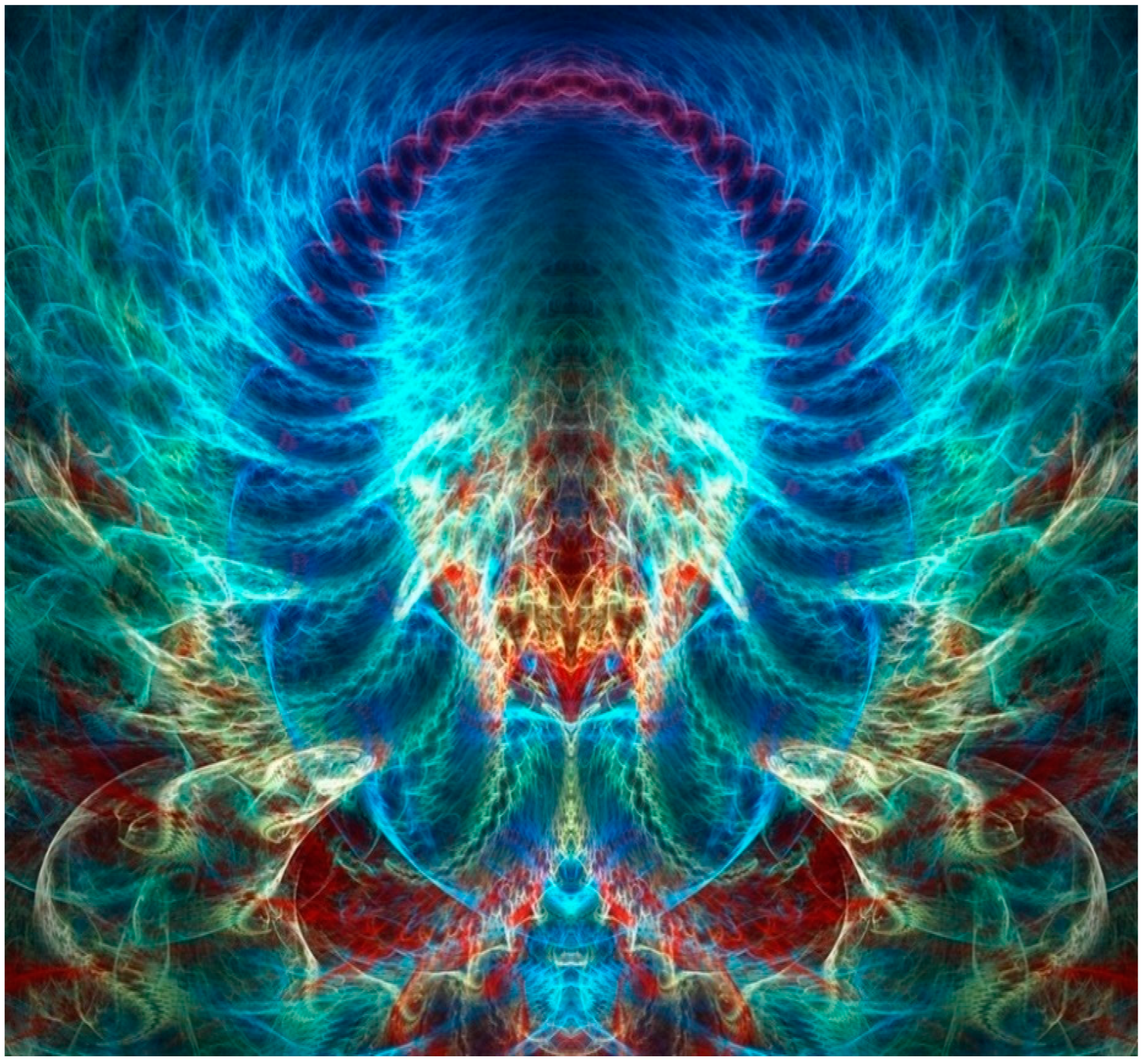
Ex. (46) shows that at this level of consideration, the curved area of the 2⁶-λ_m,n-vacuum is a complex interweaving of the 16-“colored” geodesic lines (see Figure 7). In this case, the 16-strains of the same section of the 2⁶-λ_m,n-vacuum are described by the strain tensor (63) in [3].

At the same time, the equation of geodesic lines (46) can be represented in the form.

$$\frac{d^2{x}^l}{d{s}^2}=-\frac{1}{\sqrt{16}}\left({\sum }_{q=1}^{16}{\eta }_q{Г}_{ij}^{l\left(q\right)}\right)\frac{d{x}^i}{ds}\frac{d{x}^j}{ds},$$

(50)

which defines the field of 4-accelerations $d^2{x}^l/d{s}^2$, i.e., total massless force field (see Figure 7)

$$\frac{d^2{x}^l}{d{s}^2}=\frac{1}{\sqrt{16}}{\sum }_{q=1}^{16}{\eta }_q\frac{d^2{x}^{l\left(q\right)}}{d{s}^2}{=f}^l/m_b,$$

(51)

where $m_b$ is the mass of the body that is carried away by the total (more precisely averaged) accelerated flow.

Figure 7. Fractal illustration of the interweaving of 16-“colored” geodesic lines, (i.e., accelerated streams or currents) forming the fabric of the 2⁶-λ_m,n-vacuum.

Figure 7. Fractal illustration of the interweaving of 16-“colored” geodesic lines, (i.e., accelerated streams or currents) forming the fabric of the 2⁶-λ_m,n-vacuum.

The next level of consideration is the 2¹⁰-λ_m,n-vacuum, which is considered as the result of the interweaving of not 16, but 256 metric intra-vacuum layers (see §2.9 in [2] and § 5.3 in [3]). In this case, the curved area of 2⁶-λ_m,n-vacuum is the result of averaging 265-deformations of the curved area of the 2¹⁰-λ_m,n-vacuum, just as the curved area of the 2³-λ_m,n-vacuum is the result of averaging 16-deformations of the curved area 2⁶-λ_m,n-vacuum.

A more sophisticated consideration of the curvature of the λ_m,n-vacuum area can be continued to infinity by a multiple of 2^k (see § 2.9 in [2]). In this case, each time the metric-dynamics of the subsequent transverse level of consideration of the 2^k-λ_m,n-vacuum is the result of averaging (i.e., in fact, coarsening) of the metric-dynamics of the previous, much more finely and elegantly arranged level 2^k+l-λ_m,n-vacuum.

3. Different Directions of Development of Dynamics of a λ_m,n-Vacuum Layers

As part of the development of the general dynamics of λ_m,n-vacuum layers, a number of other possibilities should be considered that may be useful for solving various metric-dynamic problems of geometrized vacuum physics.

The expanded dynamics of a two-sided 2³-λ_m,n-vacuum is based on a functional of the form (8)

$$S={\int }_{p1}^{p2}d{s}^{\left(\pm \right)}=\frac{1}{\sqrt{2}}{\int }_{p1}^{p2}\left(d{s}^{\left(+\right)}+id{s}^{\left(-\right)}\right),$$

however, the linear forms $d{s}^{\left(+\right)}\mathrm{a}\mathrm{n}\mathrm{d}d{s}^{\left(-\right)}$ can be represented in different ways, depending on the task and the depth of consideration. Below are several

(1). Let’s return to the simplest level of consideration of the curved two-sided area of the 2³-λ_m,n-vacuum. In this case, instead of the system of metrics (1), the outer and inner sides (i.e., subcont and antisubcont) of the curved area of the 2³-λ_m,n-vacuum are described by conjugate metrics

$$\left\{\begin{array}{c}d{s}^{(+)2}=g_{ij}^{(+)}d{x}^{i}d{x}^j\mathrm{with}\mathrm{signature}\left(+---\right),\\ d{s}^{(-)2}=g_{ij}^{(-)}d{x}^{i}d{x}^j\mathrm{with}\mathrm{signature}\left(-+++\right),\end{array}\right.$$

(52)

which, according to Exs. (13) – (14), can be represented as scalar products of vectors $d{\mathbf{s}}^{\left(a\right)}\mathrm{a}\mathrm{n}\mathrm{d}d{\mathbf{s}}^{\left(b\right)}$

$$\left\{\begin{array}{c}d{s}^{(+)2}=d{\mathbf{s}}^{\left(a\right)}d{\mathbf{s}}^{\left(b\right)}\mathrm{with}\mathrm{signature}\left(+---\right),\\ d{s}^{(-)2}=d{\mathbf{s}}^{\left(c\right)}d{\mathbf{s}}^{\left(d\right)}\mathrm{with}\mathrm{signature}(-+++),\end{array}\right.$$

(53)

where, for example,

ds^(a)= β^pm(a)e_m^(а)α_pi^(a)dxⁱ with signature {– – – –}
ds^(b) = β^ln(b)e_n^(b)α_lj^(b)dx^j with signature {– + + +}
ds^(c) = β^pm(с)e_m^(с)α_pi^(с)dxⁱ with signature {+ + + +}
ds^(d) = β^ln(d)e_n^(d)α_lj^(d)dx^j with signature {– + + +}.

(54)

We find variations of all possible binary scalar products of vectors (54)

δ(ds^(a)ds^(b)) = δ(ds^(a))ds^(b) + ds^(a)δ(ds^(b)) with signature (+ – – –)
δ(ds^(c)ds^(d)) = δ(ds^(c))ds^(d) + ds^(c)δ(ds^(d)) with signature (– + + +)
δ(ds^(a)ds^(с)) = δ(ds^(a))ds^(с) + ds^(a)δ(ds^(с)) with signature (– – – –)
δ(ds^(c)ds^(b)) = δ(ds^(c))ds^(b) + ds^(c)δ(ds^(b)) with signature (– + + +)
δ(ds^(a)ds^(d)) = δ(ds^(a))ds^(d) + ds^(a)δ(ds^(d)) with signature (+ – – –)
δ(ds^(d)ds^(b)) = δ(ds^(d))ds^(b) + ds^(d)δ(ds^(b)) with signature (+ + + +).

(55)

Among them there are only four variations with different signatures

δ(ds^(c)ds^(d)) = δ (ds^(c))ds^(d) + ds^(c)δ(ds^(d)) with signature (– + + +)
δ(ds^(d)ds^(b)) = δ (ds^(d))ds^(b) + ds^(d)δ(ds^(b)) with signature (+ + + +)
δ(ds^(a)ds^(b)) = δ (ds^(a))ds^(b) + ds^(a)δ(ds^(b)) with signature (+ – – –)
δ(ds^(a)ds^(с)) = δ (ds^(a))ds^(с) + ds^(a)δ(ds^(с)) with signature (– – – –).

(56)

We equate the variations of the following functionals to zero

δ ∫ds^(a)= δ ∫ β^pm(a)e_m^(а)α_pi^(a)dxⁱ = ∫(δβ^pm(a)e_m^(а)α_pi^(a)dxⁱ+ β^pm(a)δe_m^(а)α_pi^(a)dxⁱ+β^pm(a)e_m^(а)δα_pi^(a)dxⁱ + β^pm(a)e_m^(а)α_pi^(a)δdxⁱ) = 0,
δ ∫ds^(b)= δ ∫ β^pm(b)e_m^(b)α_pi^(b)dxⁱ = ∫(δβ^ln(b)e_n^(b)α_lj^(b)dx^j + β^ln(b)δe_n^(b)α_lj^(b)dx^j + β^ln(b)e_n^(b)δα_lj^(b)dx^j + β^ln(b)e_n^(b)α_lj^(b)δdx^j) = 0,
δ ∫ds^(c)= δ ∫ β^pm(c)e_m^(c)α_pi^(c)dxⁱ = ∫(δβ^pm(с)e_m^(с)α_pi^(с)dx ⁱ+ β^pm(с)δe_m^(с)α_pi^(с)dxⁱ + β^pm(с)e_m^(с)δα_pi^(с)dx ⁱ+ β^pm(с)e_m^(с)α_pi^(с)δdxⁱ) = 0,
δ ∫ds^(d)= δ ∫ β^pm(d)e_m^(d)α_pi^(d)dxⁱ = ∫(δβ^ln(d)e_n^(d)α_lj^(d)dx^j + β^ln(d)δe_n^(d)α_lj^(d)dx^j + β^ln(d)e_n^(d)δα_lj^(d)dx^j + β^ln(d)e_n^(d)α_lj^(d)δdx^j) = 0.

(57)

Ex. (57) can be represented as

δ∫ds^(a) = ∫δβ^pm(a)e_m^(а)α_pi^(a)dxⁱ + ∫β^pm(a)δem^(а)α_pi^(a)dxⁱ + ∫β^pm(a)e_m^(а)δα_pi^(a)dxⁱ + ∫β^pm(a)e_m^(а)α_pi^(a)δdxⁱ = 0,
δ∫ds^(b) = ∫δβ^ln(b)e_n^(b)α_lj^(b)dx^j + ∫β^ln(b)δen^(b)α_lj^(b)dx^j + ∫β^ln(b)e_n^(b)δα_lj^(b)dx^j + ∫β^ln(b)e_n^(b)α_lj^(b)δdx^j = 0,
δ∫ds^(c) = ∫δβ^pm(c)e_m^(c)α_pi^(c)dxⁱ + ∫β^pm(c)δem^(c)α_pi^(c)dxⁱ + ∫β^pm(c)e_m^(c)δα_pi^(c)dxⁱ + ∫β^pm(c)e_m^(c)α_pi^(c)δdxⁱ = 0,
δ∫ds^(d) = ∫δβ^ln(d)e_n^(d)α_lj^(d)dx^j + ∫β^ln(d)δen^(d)α_lj^(d)dx^j + ∫β^ln(d)e_n^(d)δα_lj^(d)dx^j + ∫β^ln(d)e_n^(d)α_lj^(d)δdx^j = 0.

(58)

Here, all possible changes (distortions, deformations and displacements) of the 4-bases e_m^(а), for example, those shown in Figure 4b.

Substituting variations (58) into Exs. (56), and finding equations for the extremals of these functionals, we obtain 32 types of different accelerations (or massless force effects).

(2). In §10 in [2], the spintensor representation of metrics with various signatures was considered. For example, let’s write the diagonal quadratic form with the signature (+ – – –) in the following form

$$\begin{gathered} d{s}^{\left(+\right)2}=g_{00}d{x}^{0}d{x}^0-g_{11}d{x}^{1}d{x}^1-g_{22}d{x}^{2}d{x}^2-g_{33}d{x}^{3}d{x}^3= \\ ={\left(\begin{array}{cc}{q}_{0}d{x}^0+q_{3}d{x}^3& q_{1}d{x}^1+i{q}_{2}d{x}^2\\ q_{1}d{x}^1-i{q}_{0}d{x}^0& q_{0}d{x}^0-q_{3}d{x}^3\end{array}\right)}_{det}, \end{gathered}$$

(59)

where $q_i=\sqrt{g_{ii}}$.

This A4 matrix can be represented as a linear form

$$\begin{gathered} A_4^{(+---)}=\left(\begin{array}{cc}{q}_{0}d{x}^0+q_{3}d{x}^3& q_{1}d{x}^1+i{q}_{2}d{x}^2\\ q_{1}d{x}^1-i{q}_{0}d{x}^0& q_{0}d{x}^0-q_{3}d{x}^3\end{array}\right)= \\ =q_{0}d{x}^0\left(\begin{array}{cc}1& 0\\ 0& 1\end{array}\right)-q_{1}d{x}^1\left(\begin{array}{cc}0& -1\\ -1& 0\end{array}\right)-q_2{dx}^2\left(\begin{array}{cc}0& -i\\ i& 0\end{array}\right)-q_{3}d{x}^3\left(\begin{array}{cc}-1& 0\\ 0& 1\end{array}\right). \end{gathered}$$

(60)

In this case, the dynamics of a 2³-λ_m,n-vacuum layer with signature (+ – – –) can be determined by the equality to zero of the first variation of the functional of the form

$${\int }_{{\mathrm{p}}_1}^{{\mathrm{p}}_2}{A}_4^{(+---)}={\int }_{{\mathrm{p}}_1}^{{\mathrm{p}}_2}\left(q_{0}d{x}^0\left(\begin{array}{cc}1& 0\\ 0& 1\end{array}\right)-q_{1}d{x}^1\left(\begin{array}{cc}0& -1\\ -1& 0\end{array}\right)-q_2{dx}^2\left(\begin{array}{cc}0& -i\\ i& 0\end{array}\right)-q_{3}d{x}^3\left(\begin{array}{cc}-1& 0\\ 0& 1\end{array}\right)\right)=0,$$

(61)

The dynamics of all other 2³-λ_m,n-vacuum layers are determined similarly (see Table 1 in §10 in [2]) with all possible signatures from matrix (35).

(3). In §12 in [2] the Dirac representation of a diagonal quadratic form is considered, for example, with signature (+ + + +)

ds²= g₀₀dx⁰dx⁰ + g₁₁dx¹dx¹ + g₂₂dx²dx² + g₃₃dx³dx³

(62)

as a product of two affine (linear) forms

ds² = ds’ds”= (γ₀q₀dx⁰′ + γ₁q₁dx¹′ + γ₂q₂dx²′ + γ₃q₃dx²′)·(γ₀q₀dx⁰” + γ₁q₁dx¹” + γ₂q₂dx²”+ γ₃q₃dx²”),

(63)

where $q_i=\sqrt{g_{ii}};$

γ_μ is objects satisfying the anticommutative relation of the Clifford algebra

γ_μγ_η + γ _η γ_μ = 2δ_μη.

(64)

Condition (64) is satisfied, for example, by the following set of 4×4-Dirac matrices:

$${\gamma }_0=\left(\begin{array}{cccc}1& 0& 0& 0\\ 0& 1& 0& 0\\ 0& 0& -1& 0\\ 0& 0& 0& -1\end{array}\right),{\gamma }_1=\left(\begin{array}{cccc}0& 0& 0& 1\\ 0& 0& 1& 0\\ 0& 1& 0& 0\\ 1& 0& 0& 0\end{array}\right),{\gamma }_2=\left(\begin{array}{cccc}0& 0& 0& -i\\ 0& 0& i& 0\\ 0& -i& 0& 0\\ i& 0& 0& 0\end{array}\right),{\gamma }_3=\left(\begin{array}{cccc}0& 0& 1& 0\\ 0& 0& 0& -1\\ 1& 0& 0& 0\\ 0& -1& 0& 0\end{array}\right),{\delta }_{\mu \eta }=\left(\begin{array}{cccc}1& 0& 0& 0\\ 0& 1& 0& 0\\ 0& 0& 1& 0\\ 0& 0& 0& 1\end{array}\right).$$

Also, the diagonal quadratic form (62) with signature (+ + + +) can be represented as

$$ds\equiv \sqrt{\left(d{s}_{ii}^2\right)}=\left(\begin{array}{cccc}\sqrt{d{s}_{00}^2}& 0& 0& 0\\ 0& \sqrt{d{s}_{11}^2}& 0& 0\\ 0& 0& \sqrt{d{s}_{22}^2}& 0\\ 0& 0& 0& \sqrt{d{s}_{33}^2}\end{array}\right)=\sqrt{\frac{1}{2}{\sum }_{\mu =0}^3{\sum }_{\mu =0}^3\left({\gamma }_{\mu }{\gamma }_{\eta }+{\gamma }_{\eta }{\gamma }_{\mu }\right)d{x}^{\mu }d{x}^{\eta }}.$$

(65)

The variation of the product of two linear forms (63) is equal to

δ(ds’ds”) = δ (ds’)ds”+ ds’δ(ds”).

(66)

In this case, the dynamics of a 2³-λ_m,n-vacuum layer with signature (+ + + +) is determined by the system of equations

$$\left\{\begin{array}{c}ds’=({\gamma }_0{q}_{0}d{x}^0’+{\gamma }_1{q}_{2}d{x}^1’+{\gamma }_2{q}_{2}d{x}^2’+{\gamma }_3{q}_{3}d{x}^3’)=0,\\ ds”=({\gamma }_0{q}_{0}d{x}^0”+{\gamma }_1{q}_{2}d{x}^1”+{\gamma }_2{q}_{2}d{x}^2”+{\gamma }_3{q}_{3}d{x}^3”)=0.\end{array}\right.$$

(67)

The dynamics of all other 2³-λ_m,n-vacuum layers with all possible signatures (35) are determined similarly, see §12 in [2].

Further development of various options for the dynamics of vacuum layers, based on different methods of representing quadratic forms with different signatures (35) in the form of two linear forms with different signatures (3) in [1] can significantly enrich the mathematical apparatus of the Algebra of Signature for describing complex intra-vacuum structures and processes. Perhaps these areas of the calculus of variations will interest mathematicians with the hope that they will be in demand by physicists.

Looking significantly ahead, we note that for the geometrization of most branches of modern physics based on the Algebra of Signatures, simplifications related to Riemannian geometry (see Figure 4a) are sufficient. This will be shown in the following articles of this series. However, to geometrize psychophysical phenomena, it is necessary to develop the most complex version of differential geometry: – the geometry of absolute parallelism (see Figure 4b) [4,6] with using the Algebra of Signature, i.e., taking into account the totality of distortions of all 16 types of affine spaces with different stignatures (3) in [1]

$$stign\left(e_i^{\left(a\right)}\right)=\left(\begin{array}{cccc}\left\{++++\right\}& \left\{+++-\right\}& \left\{-++-\right\}& \left\{++-+\right\}\\ \left\{---+\right\}& \left\{-+++\right\}& \left\{--++\right\}& \left\{-+-+\right\}\\ \left\{+--+\right\}& \left\{++--\right\}& \left\{+---\right\}& \left\{+-++\right\}\\ \left\{--+-\right\}& \left\{+-+-\right\}& \left\{-+--\right\}& \left\{----\right\}\end{array}\right).$$

(68)

4. Dynamics of a Two-Sided 2³-λ_m,n-vacuum In a State of Constant Curvature

4.1. Stationary Metric in Riemannian Geometry

Let’s continue considering metrics (52)

$$\left\{\begin{array}{c}d{s}^{(+)2}=g_{ij}^{(+)}d{x}^{i}d{x}^j\mathrm{with}\mathrm{signature}\left(+---\right)-\mathrm{metric}\mathrm{of}\mathit{subcont}\left(\mathrm{outer}\mathrm{side}\mathrm{of}a{2}^3-{\lambda }_{m,n}-\mathrm{vacum}\right),\\ d{s}^{(-)2}=g_{ij}^{(-)}d{x}^{i}d{x}^j\mathrm{with}\mathrm{signature}\left(-+++\right)-\mathrm{metric}\mathrm{of}\mathit{antisubcont}\left(\mathrm{iner}\mathrm{side}\mathrm{of}a{2}^3-{\lambda }_{m,n}-\mathrm{vacum}\right).\end{array}\right.$$

(69)

Everything described below applies to both metrics (69) separately, so we investigate the general case

$$d{s}^2=g_{ij}d{x}^{i}d{x}^j\leftrightarrow \left\{\begin{array}{c}ord{s}^{(+)2}=g_{ij}^{(+)}d{x}^{i}d{x}^j,\\ ord{s}^{(-)2}=g_{ij}^{(-)}d{x}^{i}d{x}^j.\end{array}\right.$$

(70)

Further in this paragraph we will partially repeat the derivation of several equations from the classical source [5], pp. 250 – 251 due to the fact that these equations are of particular importance for the vacuum dynamics developed here. In addition, the order of presentation has been expanded and changed, and a slightly different interpretation of the results obtained has been proposed.

We assume that all components of the metric tensor in metric (70) are independent of time

$$g_{ij}=const.$$

(71)

Let’s rewrite the quadratic form (70), highlighting the components with zero indices

$$d{s}^2={\mathrm{c}}^2{g}_{00}d{t}^2+2c{g}_{0\alpha }d{x}^{\alpha }dt+g_{\alpha \beta }d{x}^{\alpha }d{x}^{\beta }\leftrightarrow \left\{\begin{array}{c}ord{s}^{(+)2}={g_{00}^{(+)}\left(d{x}^0\right)}^2+2g_{0\alpha }^{(+)}d{x}^{0}d{x}^{\alpha }+g_{\alpha \beta }^{(+)}d{x}^{\alpha }d{x}^{\beta },\\ ord{s}^{(-)2}={g_{00}^{(-)}\left(d{x}^0\right)}^2+2g_{0\alpha }^{(-)}d{x}^{0}d{x}^{\alpha }+g_{\alpha \beta }^{(-)}d{x}^{\alpha }d{x}^{\beta },\end{array}\right.$$

(72)

where α, β = 1, 2, 3; dx⁰ = cdt.

4.2. Velocity of a Local Region of Metric Space

Let’s determine the speed of movement of a local region of the metric space (in particular, subcont or antisubcont), the metric-dynamic properties of which are determined by the stationary metric (72).

To do this, to the right side of the generalized metric (72) we add and subtract the quantity

$${\left(\frac{g_{0\alpha }d{x}^{\alpha }}{\sqrt{g_{00}}}\right)}^2=\frac{g_{0\alpha }{g}_{0\beta }}{g_{00}}d{x}^{\alpha }d{x}^{\beta },$$

(73)

as a result, we get

$$d{s}^2={\mathrm{c}}^2{\left[\sqrt{g_{00}}dt+\frac{g_{0\alpha }d{x}^{\alpha }}{c\sqrt{g_{00}}}\right]}^2-\left[-g_{\alpha \beta }+\frac{g_{0\alpha }{g}_{0\beta }}{g_{00}}\right]d{x}^{\alpha }d{x}^{\beta },$$

(74)

whence for the studied area of space we have an analogue of proper time [5]

$$d\tau =\sqrt{g_{00}}dt+\frac{g_{0\alpha }d{x}^{\alpha }}{c\sqrt{g_{00}}}\mathrm{or}d\tau =\frac{\sqrt{g_{00}}}{\mathrm{c}}\left(d{x}^0+\frac{g_{0\alpha }}{g_{00}}d{x}^{\alpha }\right).$$

(75)

The second term in Ex. (74) is the square of the distance between two points in a 3-dimensional metric space (in this case, in a 3-dimensional subcount or in a 3-dimensional antisubcount)

$$d{l}^2=-\left[g_{\alpha \beta }-\frac{g_{0\alpha }{g}_{0\beta }}{g_{00}}\right]d{x}^{\alpha }d{x}^{\beta }\mathrm{or}d{l}^2={\gamma }_{\alpha \beta }d{x}^{\alpha }d{x}^{\beta },$$

(76)

where the 3-dimensional spatial metric tensor is introduced

$${{\gamma }_{\alpha \beta }=-g}_{\alpha \beta }+\frac{g_{0\alpha }{g}_{0\beta }}{g_{00}}.$$

(77)

Metric (74) taking into account Exs. (75) and (76) takes the form

$$d{s}^2={\mathrm{c}}^{2}d{\tau }^2-d{l}^2,$$

(78)

which corresponds to the reference system in which the local area under study of one of the sides of the 2³-λ_m,n-vacuum (in particular, subcont or antisubcont) is at rest.

Now we can introduce the 3-dimensional speed of movement of a local region of the metric space (in this case, subcont or antisubcont), the metric-dynamic properties of which are specified by the components of the metric tensor from metric (72). We divide the distance (76) by the time (75), as a result we obtain the modulus of the velocity vector

$$\left|\overrightarrow{v}\right|=\frac{dl}{d\tau }=\frac{cdl}{\sqrt{g_{00}}\left(x^0+\frac{g_{0\alpha }}{g_{00}}d{x}^{\alpha }\right)}=\frac{c\sqrt{\left(-g_{\alpha \beta }+\frac{g_{0\alpha }{g}_{0\beta }}{g_{00}}\right)d{x}^{\alpha }d{x}^{\beta }}}{\sqrt{g_{00}}\left(x^0+\frac{g_{0\alpha }}{g_{00}}d{x}^{\alpha }\right)}$$

(79)

with components [5], p. 250

$$v^{\alpha }=\frac{cd{x}^{\alpha }}{\sqrt{g_{00}}\left(x^0+\frac{g_{0\alpha }}{g_{00}}d{x}^{\alpha }\right)}.$$

(80)

The covariant components of the velocity vector $v_{\alpha }$ are determined by the Expressions [5], p. 250

$$v_{\alpha }={\gamma }_{\alpha \beta }{v}^{\beta },v^2=v_{\alpha }{v}^{\beta },$$

Taking into account Ex. (79), the stationary metric (72) can be represented as [5], p. 250

$$d{s}^2=g_{00}{\left(d{x}^0-g_{\alpha }d{x}^{\alpha }\right)}^2\left(1-\frac{v^2}{{\mathrm{c}}^2}\right),$$

(81)

where the 3-dimensional vector is introduced

$$g_{\alpha }=-\frac{g_{0\alpha }}{g_{00}}.$$

(82)

The 4-speed components $u^i=\frac{d{x}^i}{ds}$, taking into account Ex. (81) are equal [5], p. 251

$$u^0=\frac{1}{\sqrt{g_{00}}\sqrt{1-\frac{v^2}{c^2}}}+\frac{g_{\alpha }{v}^{\alpha }}{c\sqrt{1-\frac{v^2}{c^2}}},u^{\alpha }=\frac{v^{\alpha }}{c\sqrt{1-\frac{v^2}{c^2}}}.$$

(83)

4.3. Acceleration of a Local Region of Metric Space

Let’s find the acceleration of a local region of the metric space (in particular, subcont or antisubcont), the metric-dynamic properties of which are determined by the stationary metric (72).

As was shown in §1.1, the acceleration of a local region of the metric space with simplifications related to Riemannian geometry is given by Equation (26)

$$\frac{d^2{x}^l}{d{s}^2}=-{Г}_{ij}^l\frac{d{x}^i}{ds}\frac{d{x}^j}{ds},$$

(84)

We find Christoffel symbols (25)

$${Г}_{ij}^l=\frac{1}{2}{g}^{l\mu }\left(\frac{\partial g_{\mu i}}{\partial x^j}+\frac{\partial g_{\mu j}}{\partial x^i}-\frac{\partial g_{ij}}{\partial x^{\mu }}\right)$$

(85)

for the considered stationary case.

Let’s substitute the components of the metric tensor from the stationary metric (72) into Ex. (85). As a result, taking into account conditions (71), we obtain the following non-zero components of this pseudo-tensor [5], p. 251

$${Г}_{00}^{\alpha }=½g_{00}^{;\alpha },$$

(86)

$${Г}_{0\beta }^{\alpha }=½g_{00}\left(g_{;\beta }^{\alpha }-g_{\beta }^{;\alpha }\right)-½g_{\beta }{g}_{00}^{;\alpha },$$

(87)

$${Г}_{\beta \gamma }^{\alpha }={\lambda }_{\beta \gamma }^{\alpha }+½g_{00}\left[g_{\beta }\left(g_{\beta }^{;\alpha }-g_{\beta }^{;\alpha }\right)+g_{\gamma }\left(g_{;\beta }^{\alpha }-g_{;\beta }^{\alpha }\right)\right]+½g_{\beta }{g}_{\gamma }{g}_{00}^{;\alpha },$$

(88)

where, for example, $g_{\gamma }^{;\alpha }$ is the covariant derivative, which in this case coincides with the partial derivative [5]:

$$g_{;\gamma }^{\alpha }=\frac{\partial g^{\alpha }}{\partial x^{\gamma }}+{Г}_{k\gamma }^{\alpha }{g}^k=\frac{\partial g^{\alpha }}{\partial x^{\gamma }};$$

(89)

${\lambda }_{\beta \gamma }^{\alpha }$ is a 3-dimensional Christoffel symbol composed of components of the metric tensor $g_{\alpha \beta }$ in the same way as ${Г}_{ij}^l$ is composed of components $g_{ij}$.

In Ex. (86) – (89) all tensor actions (covariant differentiation, raising and lowering indices) are performed in a 3-dimensional space with a metric $g_{\alpha \beta }$ over a 3-dimensional vector $g_{\alpha }$ and a scalar $g_{00}$.

Let’s substitute Ex. (86) – (89) into the equation of motion (84), as a result we obtain [5], p. 251

$$\frac{d{u}^{\alpha }}{ds}=-{Г}_{00}^{\alpha }{\left(u^0\right)}^2-2{Г}_{0\beta }^{\alpha }{u}^0{u}^{\beta }-{Г}_{\beta \gamma }^{\alpha }{u}^{\alpha }{u}^{\gamma }.$$

(90)

After transforming Ex. (90) using 4-speed components (83) and Christoffel symbols (86) – (89), we obtain [5], p. 251

$$\frac{d{u}^a}{ds}=\frac{d}{ds}\frac{{\nu }^{\alpha }}{\mathrm{c}\sqrt{1-\frac{{\nu }^2}{{\mathrm{c}}^2}}}=-\frac{g_{00}^{;\alpha }}{2g_{00}\left(1-\frac{{\nu }^2}{c^2}\right)}-\frac{\sqrt{g_{00}}\left(g_{;\beta }^{\alpha }-g_{\beta }^{;\alpha }\right){\nu }^{\beta }}{c\left(1-\frac{{\nu }^2}{c^2}\right)}-\frac{{\lambda }_{\beta \gamma }^{\alpha }{\nu }^{\beta }{\nu }^{\gamma }}{c^2\left(1-\frac{{\nu }^2}{c^2}\right)}.$$

(91)

In the general theory of relativity, based on Riemannian geometry, the force acting on a particle with momentum p = mv (where m is the mass of the particle, v is the speed of the flow entraining the particle) is defined as a 3-dimensional covariant differential [5], p. 251

$$f^{\alpha }=c\sqrt{1-\frac{{\nu }^2}{{\mathrm{c}}^2}}\frac{D{p}^{\alpha }}{ds}=c\sqrt{1-\frac{{\nu }^2}{{\mathrm{c}}^2}}\frac{d}{ds}\frac{{m\nu }^{\alpha }}{\sqrt{1-\frac{{\nu }^2}{{\mathrm{c}}^2}}}+{\lambda }_{\beta \gamma }^{\alpha }\frac{{m\nu }^{\beta }{\nu }^{\gamma }}{\sqrt{1-\frac{{\nu }^2}{{\mathrm{c}}^2}}}.$$

(92)

Let’s divide the components of the force vector (92) by the particle mass m. As a result, we obtain the rooms of the acceleration vector of the local region of the metric space (in particular, subcont or antisubcont)

$$\frac{f^{\alpha }}{m}=a^{\alpha }=c\sqrt{1-\frac{{\nu }^2}{{\mathrm{c}}^2}}\frac{d}{ds}\frac{{\nu }^{\alpha }}{\sqrt{1-\frac{{\nu }^2}{{\mathrm{c}}^2}}}+\frac{{\lambda }_{\beta \gamma }^{\alpha }{\nu }^{\beta }{\nu }^{\gamma }}{\sqrt{1-\frac{{\nu }^2}{{\mathrm{c}}^2}}}.$$

(93)

components of the acceleration vector (93), taking into account Ex. (91), can be represented in the form (for convenience, the index α is omitted) [5], p. 252

$$a_{\alpha }=\frac{c^2}{\sqrt{1-\frac{{\nu }^2}{c^2}}}\left\{-\frac{\partial \mathit{ln}\sqrt{g_{00}}}{\partial x^a}+\sqrt{g_{00}}\left(\frac{\partial g_{\beta }}{\partial x^a}-\frac{\partial g_{\alpha }}{\partial x^{\beta }}\right)\frac{v^{\beta }}{c}\right\},$$

(94)

or in conventional three-dimensional vector notation [5], p. 252

$$\overrightarrow{a}=\frac{c^2}{\sqrt{1-\frac{v^2}{c^2}}}\left\{-grad\left(\mathit{ln}\sqrt{g_{00}}\right)+\sqrt{g_{00}}\left[\frac{\overrightarrow{v}}{c}\times rot\overrightarrow{g}\right]\right\},$$

(95)

where $\overrightarrow{g}(g_1,g_2,g_3)$ is a 3-dimensional vector with components

$$g_{\alpha }=-\frac{g_{0\alpha }}{g_{00}}.$$

(96)

In the note by Landau L.D. and Lifshits E.M. noted that in three-dimensional curvilinear coordinates $rot\overrightarrow{g}$ should be understood in the same sense as the vector dual to the tensor $\left(\frac{\partial g_{\beta }}{\partial x^a}-\frac{\partial g_{\alpha }}{\partial x^{\beta }}\right)$, so that its contravariant components should be written in the form [5], p 252

$${\left(rot\overrightarrow{g}\right)}^{\gamma }=\frac{1}{2\sqrt{\gamma }}{e}^{\alpha \beta \gamma }\left(\frac{\partial g_{\beta }}{\partial x^a}-\frac{\partial g_{\alpha }}{\partial x^{\beta }}\right),$$

(97)

where $\sqrt{\gamma }$ is the determinant of the spatial metric tensor (77);

$e^{\alpha \beta \gamma }=e^{123}=e_{123}$= 1, and when two symbols are rearranged, the sign changes.

$$\overrightarrow{v}=\frac{d\overrightarrow{l}}{d\tau }=\frac{cd\overrightarrow{l}}{\sqrt{g_{00}}\left(d{x}^0+\frac{g_{\alpha \beta }}{g_{00}}d{x}^{\alpha }\right)}$$

(98)

is vector of the 3-dimensional velocity of a local region of a metric space (in particular, subcont or antisubcont) with components (80)

$$v^1=\frac{cd{x}^1}{\sqrt{g_{00}}\left(x^0+\frac{g_{01}}{g_{00}}d{x}^1\right)},v^2=\frac{cd{x}^2}{\sqrt{g_{00}}\left(x^0+\frac{g_{02}}{g_{00}}d{x}^2\right)},v^3=\frac{cd{x}^3}{\sqrt{g_{00}}\left(x^0+\frac{g_{03}}{g_{00}}d{x}^3\right)}.$$

(99)

We note once again that the formula for the acceleration vector (95) was borrowed from the classical source [5], pp. 250 – 251, where it was obtained within the framework of Riemannian geometry (see Figure 4a), and under the condition that the metric is stationary (72), i.e., when the components of the metric tensor are independent of time (71) $g_{ij}=const$.

4.4. Acceleration of a Local Section of 2³-λ_m,n-Vacuum

If we perform all operations (71) – (98) separately with each of the metrics (69), we obtain two acceleration vectors:

$${\mathbf{a}}^{(+)}={\overrightarrow{a}}^{(+)}=\frac{c^2}{\sqrt{1-\frac{v^{(+)2}}{c^2}}}\left\{-grad\left(\mathit{ln}\sqrt{g_{00}^{(+)}}\right)+\sqrt{g_{00}^{(+)}}\left[\frac{{\overrightarrow{v}}^{(+)}}{c}\times rot{\overrightarrow{g}}^{(+)}\right]\right\}$$

(100)

is acceleration vector of the local region of the subcont (i.e., the outer side of the 2³-λ_m,n-vacuum);

$${\mathbf{a}}^{(-)}={\overrightarrow{a}}^{(-)}=\frac{c^2}{\sqrt{1-\frac{v^{(-)2}}{c^2}}}\left\{-grad\left(\mathit{ln}\sqrt{g_{00}^{(-)}}\right)+\sqrt{g_{00}^{(-)}}\left[\frac{{\overrightarrow{v}}^{(-)}}{c}\times rot{\overrightarrow{g}}^{(-)}\right]\right\}$$

(101)

is acceleration vector of the local region of the antisubcont (i.e., the inner side of the 2³-λ_m,n-vacuum).

Acceleration of a local region of the 2³-λ_m,n-vacuum (32)

$$\frac{d^2{x}^l}{d{s}^2}=-\frac{1}{\sqrt{2}}\left({Г}_{ij}^{l\left(+\right)}\frac{d{x}^i}{ds}\frac{d{x}^j}{ds}+i{Г}_{ij}^{l\left(-\right)}\frac{d{x}^i}{ds}\frac{d{x}^j}{ds}\right),$$

(102)

can be represented in the form

$$a^{(\pm )l}=\frac{1}{\sqrt{2}}\left(a^{(+)l}+i{a}^{(-)l}\right),$$

(103)

or with indexes omitted

$$a_{\alpha }^{(\pm )}=\frac{1}{\sqrt{2}}\left(a_{\alpha }^{(+)}+i{a}_{\alpha }^{(-)}\right),$$

(104)

where in the stationary case under consideration, according to Ex. (94),

$$a_{\alpha }^{(+)}=\frac{c^2}{\sqrt{1-\frac{v^{(+)2}}{c^2}}}\left\{-\frac{\partial \mathit{ln}\sqrt{g_{00}^{(+)}}}{\partial x^a}+\sqrt{g_{00}^{(+)}}\left(\frac{\partial g_{\beta }^{(+)}}{\partial x^a}-\frac{\partial g_{\alpha }^{(+)}}{\partial x^{\beta }}\right)\frac{v^{(+)\beta }}{c}\right\},$$

(105)

$$a_{\alpha }^{(-)}=\frac{c^2}{\sqrt{1-\frac{v^{(-)2}}{c^2}}}\left\{-\frac{\partial \mathit{ln}\sqrt{g_{00}^{(-)}}}{\partial x^a}+\sqrt{g_{00}^{(-)}}\left(\frac{\partial g_{\beta }^{(-)}}{\partial x^a}-\frac{\partial g_{\alpha }^{(-)}}{\partial x^{\beta }}\right)\frac{v^{(-)\beta }}{c}\right\}.$$

(106)

In this case, the acceleration vector of the local region of the 2³-λ_m,n-vacuum, taking into account (100) – (101) has the form

$${\mathbf{a}}^{(\pm )}=\frac{1}{\sqrt{2}}\left({\mathbf{a}}^{(+)}{i\mathbf{a}}^{(-)}\right),$$

(107)

where a^(±) = ${\overrightarrow{a}}^{\left(\pm \right)}\left(\frac{1}{\sqrt{2}}\left(a_1^{(+)}+i{a}_1^{(-)}\right),\frac{1}{\sqrt{2}}\left(a_2^{(+)}+i{a}_2^{(-)}\right),\frac{1}{\sqrt{2}}\left(a_3^{(+)}+i{a}_3^{(-)}\right)\right).$

5. Geometrized Lorentz Force

5.1. Geometricized Vectors of Eclectic Tension and Magnetic Induction

Consider the vector Ex. (95)

$$\mathbf{a}=\overrightarrow{a}=\frac{1}{\sqrt{1-\frac{v^2}{c^2}}}{c}^2\left\{-grad\left(\mathit{ln}\sqrt{g_{00}}\right)+\sqrt{g_{00}}\left[\frac{\overrightarrow{v}}{c}\times rot\overrightarrow{g}\right]\right\},$$

(108)

where $\overrightarrow{g}(-\frac{g_{01}}{g_{00}},-\frac{g_{01}}{g_{00}},-\frac{g_{01}}{g_{00}})$ is a 3-dimensional vector.

We introduce the notation

$${\mathbf{E}}_v={\overrightarrow{E}}_v={-\gamma }_{c}grad\phi ,$$

(109)

$${\mathbf{B}}_v={\overrightarrow{B}}_v={\gamma }_c\sqrt{g_{00}}rot\frac{\overrightarrow{A}}{\mathrm{c}},$$

(110)

where

$$\phi =\mathit{ln}\sqrt{g_{00}}–\mathrm{geometrized}\mathrm{scalar}\mathrm{potential};$$

(111)

$$\overrightarrow{A}=\overrightarrow{g}–\mathrm{geometrized}\mathrm{vector}\mathrm{potential};$$

(112)

$${\gamma }_c=\frac{c^2}{\sqrt{1-\frac{v^2}{c^2}}},-\mathrm{Lorentz}-\mathrm{factor}\mathrm{multiplied}\mathrm{by}{c}^2.$$

(113)

Taking into account notations (109) – (113), the acceleration vector (108) takes the form

a=E_v + [v × B_v],

(114)

Let’s compare this acceleration vector with the Lorentz force

F_l = qE+ q[v × B] or F_l /q = E + [v × B],

(115)

where

E is electric field strength vector; B is magnetic field induction vector; q is the charge of the particle.

The obvious analogy of expressions (114) and (115) allows us to consider vectors (109) and (110) as:

E_v is the geometrized vector of electric field strength with components:

$$E_{v1}={\gamma }_c\frac{\partial \mathit{ln}\sqrt{g_{00}}}{\partial x^1},E_{v2}={\gamma }_c\frac{\partial \mathit{ln}\sqrt{g_{00}}}{\partial x^2},E_{v3}={\gamma }_c\frac{\partial \mathit{ln}\sqrt{g_{00}}}{\partial x^3}.$$

(116)

B_v is the geometrized vector of magnetic induction with components:

$$B_{v1}={\gamma }_c\sqrt{g_{00}}\left(\frac{\partial g_3}{\partial x^2}-\frac{\partial g_2}{\partial x^3}\right),B_{v2}={\gamma }_c\sqrt{g_{00}}\left(\frac{\partial g_1}{\partial x^3}-\frac{\partial g_3}{\partial x^1}\right),B_{v3}={\gamma }_c\sqrt{g_{00}}\left(\frac{\partial g_2}{\partial x^1}-\frac{\partial g_1}{\partial x^2}\right).$$

(117)

where

$$g_1=-\frac{g_{01}}{g_{00}},g_2=-\frac{g_{02}}{g_{00}},g_3=-\frac{g_{03}}{g_{00}}.$$

(118)

5.2. The meaning of Geometrized Vectors of Electric Field Strength E_v and Magnetic Induction B_v

To clarify the meaning of the vectors E_vand B_v, consider the arbitrary motion of an affine space with stignature {+ + + +} (i.e., reference frame) K′ (t′,x′,y′,z′) relative to a stationary affine space with signature {+ + + +} (i.e., frame of reference) K (t,x,y,z) (see Figure 8). This well-known classical task is borrowed from [7] in full, because otherwise, establishing the meaning of the vectors E_vand B_v will be very problematic.

Figure 8. Motion of the reference frame (or affine space) К′ with signature {+ + + +}. relative the rest reference frame (or affine space) K with signature {+ + + +}

Figure 8. Motion of the reference frame (or affine space) К′ with signature {+ + + +}. relative the rest reference frame (or affine space) K with signature {+ + + +}

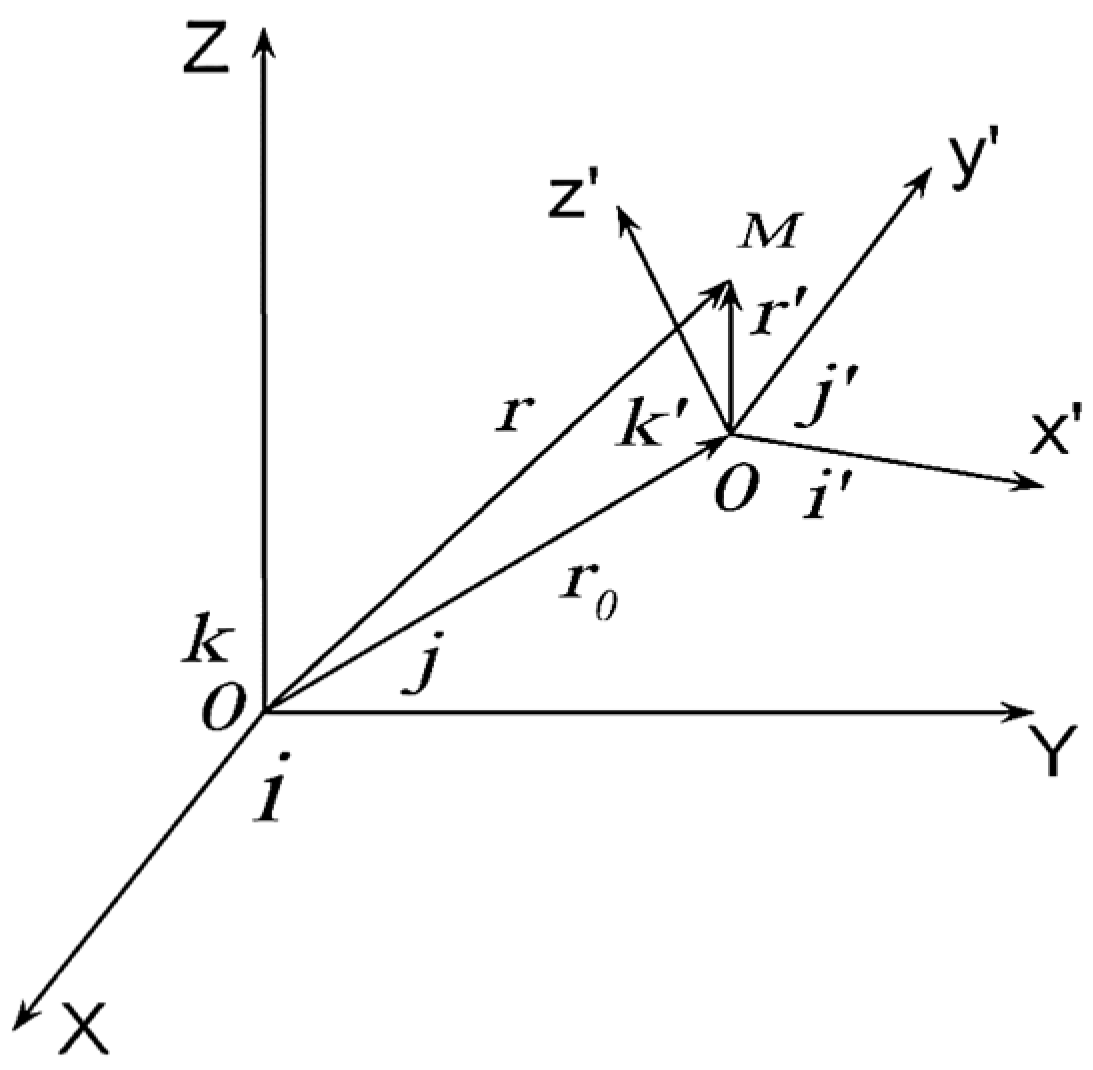
The Figure 8 shows that the radius vectors r and r, which define the position of point M in the systems K and K′ are related by the relation

r = r₀ + r′

(119)

or

ix + j y + k z = r₀ + i′ x′ + j′ y′ + k′ z′,

(120)

where

• i, j, k are orthogonal unit vectors that specify the directions of the axes of a fixed affine space K with signature {+ + +};
• i′, j′,k′ are orthogonal unit vectors that specify the directions of the axes of a moving affine space K′ with signature {+ + +}.

The speed of point M (belonging to the reference frame, or affine space, K′ ) relative to the reference frame K at t′= t is obtained as a result of differentiating both sides of Ex. (119) [7]

v_a=dr/dt = dr₀ /dt + dr′/dt,

(121)

in this case, taking into account Ex. (120) we have

v_a= v₀+ (x′ d i′/dt + y′ d j′/dt + z′ d k′/dt) + (i′dx′/dt + j′dy′/dt + k′dz′/dt).

(122)

Let the vectors i′, j′,k′ of the moving reference frame K′ can change relative to the reference frame K only due to its rotation around the point О′ with angular velocity Ω.. Therefore, the time derivatives of the unit vectors i′, j′,k′ equal to the speeds of the ends of these vectors during rotation of the reference frame К′ [7]

di′/dt = [Ω × i′], d j′/dt = [Ω × j′], d k′/dt = [Ω × k′].

(123)

Substituting Exs. (123) into Ex. (122), we obtain

v_a= v₀ + [Ω × r′] + (i′dx′/dt + j′dy′/dt + k′dz′/dt).

(124)

The acceleration of point M relative to the reference frame K at t′= t is equal to [7]

а =dv_a/dt = а_r + а_e + а_k ,

(125)

where

а_r = (i′d²x′/dt² + j′d²y′/dt² + k′d²z′/dt²) is relative acceleration;

(126)

а_е = dv₀/dt + [dΩ/dt × r′] + [Ω × [Ω × r′]] is portable acceleration;

(127)

а_k = 2[Ω × v_r] is Coriolis acceleration.

(128)

We rewrite Ex. (125) for the stationary case dv₀/dt = 0 and [dΩ/dt × r′] = 0,

а = а_pс + 2[Ω × v_r],

(129)

where

а_pс= (i′d ²x′/dt² + j′d ²y′/dt² + k′d ²z′/dt²) + [Ω × [Ω × r′]]

(130)

is stationary relative-transportable acceleration of the moving reference frame K′.

Taking into account the relation known in analytical geometry

[Ω × v_r] = – [v_r × Ω],

(131)

Ex. (129) can be represented as

а = а_pс – 2[v_r× Ω].

(132)

When comparing acceleration (132) with acceleration (114)

a=E_v + [v × В_v],

we find the following obvious analogy

E_v ≡ а_pс , B_v≡ – 2Ω , v ≡ v_r .

(133)

Thus, it turns out the following:

-

the geometrized vector of electric field strength E_v of the vacuum layer is identical to the stationary transport acceleration with torsion а_pс (130) of the local area of the moving affine space K′ in the vicinity of the point M relative to the resting affine space K;

-

the geometrized vector of magnetic induction B_v of the vacuum layer is identical to the doubled stationary angular velocity of rotation Ω of the same area of moving affine space K′ in the vicinity of the point M relative to the resting affine space K;

-

the velocity vector v of the vacuum layer corresponds to the constant displacement velocity v_r of the same area of the affine space K′ relative to the affine space K.

Within the Algebra of Signatures, each of the reference frames K′ (t′,x′,y′,z′) and K (t, x, y, z) can have any of the 16 possible bases unit vector shown in Figure 7 in [1], with the corresponding signature from matrix (68)

$$stign\left(e_i^{\left(a\right)}\right)=\left(\begin{array}{cccc}\left\{++++\right\}& \left\{+++-\right\}& \left\{-++-\right\}& \left\{++-+\right\}\\ \left\{---+\right\}& \left\{-+++\right\}& \left\{--++\right\}& \left\{-+-+\right\}\\ \left\{+--+\right\}& \left\{++--\right\}& \left\{+---\right\}& \left\{+-++\right\}\\ \left\{--+-\right\}& \left\{+-+-\right\}& \left\{-+--\right\}& \left\{----\right\}\end{array}\right)$$

Therefore, within the framework of the Algebra of Signature, 256 options for the movement of two affine spaces relative to each other are possible.

Let’s also note that the complete analogy between vectors (132) and (114) is due to the fact that they were obtained under the same stationarity dv₀/dt = 0 and [dΩ/dt × r′] = 0, and at the same simplifications corresponding to Riemannian geometry (see Figure 4a), i.e., only the displacement and rotation of the reference frame K′ are taken into account while maintaining the sizes of the basis vectors i′, j′ , k′ (or e₁^(a, e₂^{(a )}, e₃^{(a )}) and the angles between them.

A similar analysis can be performed for more complex cases, when all four parameters α_ij^(a), β^pm(a), e_m^(a), dx^j(a) both of the reference frame K′ and the reference frame K can change (see Figure 4b), and this will correspond to the more complex differential geometry, for example, such as the geometry of absolute parallelism.

6. Geometricized Vectors of Electric Field Strength and Magnetic Induction of the 2^k-λ_m,n-Vacuum

6.1. Geometricized Vectors of Electric Field Strength and Magnetic Induction of the 2³-λ_m,n-Vacuum

Let‘s return to the consideration of a stationary curved area of a two-sided 2³-λ_m,n-vacuum within the framework of the Algebra of Signature representations with simplifications related to Riemannian geometry (see Figure 4a).

In § 4.4, the acceleration vector of the stationary area of the 2³-λ_m,n-vacuum (107) was obtained

$${\mathbf{a}}^{(\pm )}=\frac{1}{\sqrt{2}}({\mathbf{a}}^{(+)}+{i\mathbf{a}}^{(-)}),$$

(134)

where, according to Exs. (100) – (101) and § 5.1,

$${\mathbf{a}}^{(+)}{\overrightarrow{a}}^{(+)}=\frac{c^2}{\sqrt{1-\frac{v^{(+)2}}{c^2}}}\left\{-grad\left(\mathit{ln}\sqrt{g_{00}^{(+)}}\right)+\sqrt{g_{00}^{(+)}}\left[\frac{{\overrightarrow{v}}^{(+)}}{c}\times rot{\overrightarrow{g}}^{(+)}\right]\right\}={{\mathit{E}}_v}^{(+)}+[{\mathit{v}}^{(+)}\times {{\mathit{B}}_v}^{(+)}],$$

(135)

$${\mathbf{a}}^{(-)}={\overrightarrow{a}}^{(-)}=\frac{c^2}{\sqrt{1-\frac{v^{(-)2}}{c^2}}}\left\{-grad\left(\mathit{ln}\sqrt{g_{00}^{(-)}}\right)+\sqrt{g_{00}^{(-)}}\left[\frac{{\overrightarrow{v}}^{(-)}}{c}\times rot{\overrightarrow{g}}^{(-)}\right]\right\}={{\mathbf{E}}_v}^{(-)}+[{\mathit{v}}^{(-)}\times {{\mathbf{B}}_v}^{(-)}].$$

(136)

Let‘s substitute the acceleration vectors (135) and (136) into Ex. (134), as a result we obtain

$${\mathbf{a}}^{(\pm )}=\frac{1}{\sqrt{2}}\{{{\mathbf{E}}_v}^{(+)}+[{\mathit{v}}^{(+)}\times {{\mathit{B}}_v}^{(+)}]+i{{\mathbf{E}}_v}^{(-)}+[{\mathit{v}}^{(-)}\times {{\mathit{B}}_v}^{(-)}\left]\right)\}.$$

(137)

or

$${\mathbf{a}}^{(\pm )}=\frac{1}{\sqrt{2}}\left\{\right({{\mathbf{E}}_v}^{(+)}+{{i\mathbf{E}}_v}^{(-)})+([{\mathit{v}}^{(+)}\times {{\mathit{B}}_v}^{(+)}]+i[{\mathbf{v}}^{(-)}\times {{\mathit{B}}_v}^{(-)}]\left)\right\}.$$

(138)

where according to expressions (116) – (118):

E_v⁽⁺⁾ is geometrized vector of the electric field strength of subcont, with components:

$$E_{v1}^{(+)}={\gamma }_c\frac{\partial \mathit{ln}\sqrt{g_{00}^{(+)}}}{\partial x^1},E_{v2}^{(+)}={\gamma }_c\frac{\partial \mathit{ln}\sqrt{g_{00}^{(+)}}}{\partial x^2},E_{v3}^{(+)}={\gamma }_c\frac{\partial \mathit{ln}\sqrt{g_{00}^{(+)}}}{\partial x^3}.$$

(139)

B_v⁽⁺⁾ is geometrized vector of the magnetic induction with of subcont, with components:

$$B_{v1}^{(+)}={\gamma }_c\sqrt{g_{00}^{(+)}}\left(\frac{\partial g_3^{(+)}}{\partial x^2}-\frac{\partial g_2^{(+)}}{\partial x^3}\right),B_{v2}^{(+)}={\gamma }_c\sqrt{g_{00}^{(+)}}\left(\frac{\partial g_1^{(+)}}{\partial x^3}-\frac{\partial g_3^{(+)}}{\partial x^1}\right),B_{v3}^{(+)}={\gamma }_c\sqrt{g_{00}^{(+)}}\left(\frac{\partial g_2^{(+)}}{\partial x^1}-\frac{\partial g_1^{(+)}}{\partial x^2}\right).$$

(140)

here

$$g_1^{(+)}=-\frac{g_{01}^{(+)}}{g_{00}^{(+)}},g_2^{(+)}=-\frac{g_{02}^{(+)}}{g_{00}^{(+)}},g_3^{(+)}=-\frac{g_{03}^{(+)}}{g_{00}^{(+)}}.$$

(141)

E_v^(–) is geometrized vector of the electric field strength of antisubcont, with components:

$$E_{v1}^{(-)}={\gamma }_c\frac{\partial \mathit{ln}\sqrt{g_{00}^{(+)}}}{\partial x^1},E_{v2}^{(-)}={\gamma }_c\frac{\partial \mathit{ln}\sqrt{g_{00}^{(-)}}}{\partial x^2},E_{v3}^{(-)}={\gamma }_c\frac{\partial \mathit{ln}\sqrt{g_{00}^{(-)}}}{\partial x^3}.$$

(142)

B_v^(–) is geometrized vector of the magnetic induction with of antisubcont, with components:

$$B_{v1}^{(-)}={\gamma }_c\sqrt{g_{00}^{(-)}}\left(\frac{\partial g_3^{(-)}}{\partial x^2}-\frac{\partial g_2^{(-)}}{\partial x^3}\right),B_{v2}^{(-)}={\gamma }_c\sqrt{g_{00}^{(-)}}\left(\frac{\partial g_1^{(-)}}{\partial x^3}-\frac{\partial g_3^{(-)}}{\partial x^1}\right),B_{v3}^{(-)}={\gamma }_c\sqrt{g_{00}^{(-)}}\left(\frac{\partial g_2^{(-)}}{\partial x^1}-\frac{\partial g_1^{(-)}}{\partial x^2}\right).$$

(143)

here

$$g_1^{(-)}=-\frac{g_{01}^{(-)}}{g_{00}^{(-)}},g_2^{(-)}=-\frac{g_{02}^{(-)}}{g_{00}^{(-)}},g_3^{(-)}=-\frac{g_{03}^{(-)}}{g_{00}^{(-)}}.$$

(144)

We recall that time-independent components of the metric tensors $g_{ij}^{(+)}=const$ and $g_{ij}^{(-)}=const$ from the conjugate stationary metrics (72):

$$\left\{\begin{array}{c}d{s}^{(+)2}={g_{00}^{(+)}\left(d{x}^0\right)}^2+2g_{0\alpha }^{(+)}d{x}^{0}d{x}^{\alpha }+g_{\alpha \beta }^{(+)}d{x}^{\alpha }d{x}^{\beta }\mathrm{is}\mathrm{metric}\mathrm{of}\mathrm{stationary}\mathit{subcont}\left(\mathrm{see}\mathrm{Figure}2\right),\\ d{s}^{(-)2}={g_{00}^{(-)}\left(d{x}^0\right)}^2+2g_{0\alpha }^{(-)}d{x}^{0}d{x}^{\alpha }+g_{\alpha \beta }^{(-)}d{x}^{\alpha }d{x}^{\beta }\mathrm{is}\mathrm{metric}\mathrm{of}\mathrm{stationary}\mathit{antisubcont}\end{array}\right.$$

(145)

are substituted into Exs. (139) – (144).

Taking into account Exs. (139) – (144), the components of the 3-dimensional acceleration vector of the stationary curved local area of the two-sided 2³-λ_m,n-vacuum a^(±) (138) are equal to the modules of complex numbers: a^(±) $\left(\left|a_1^{\left(\pm \right)}\right|,\left|a_2^{\left(\pm \right)}\right|,\left|a_3^{\left(\pm \right)}\right|\right),$where:

$$\begin{gathered} a_1^{\left(\pm \right)}=\frac{1}{\sqrt{2}}\left\{\left(E_{v1}^{(+)}+i{E}_{v1}^{(-)}\right)+\left[\left(v_2^{(+)}{B}_{v3}^{(+)}-v_3^{(+)}{B}_{v2}^{(+)}\right)+i\left(v_2^{(-)}{B}_{v3}^{(-)}-v_3^{(-)}{B}_{v2}^{(-)}\right)\right]\right\}, \\ {a}_2^{\left(\pm \right)}=\frac{1}{\sqrt{2}}\left\{\left(E_{v2}^{\left(+\right)}+i{E}_{v2}^{\left(-\right)}\right)+\left[\left(v_3^{\left(+\right)}{B}_{v1}^{\left(+\right)}-v_1^{\left(+\right)}{B}_{v3}^{\left(+\right)}\right)+i\left(v_3^{\left(-\right)}{B}_{v1}^{\left(-\right)}-v_1^{\left(-\right)}{B}_{v3}^{\left(-\right)}\right)\right]\right\}, \\ {a}_3^{\left(\pm \right)}=\frac{1}{\sqrt{2}}\left\{\left(E_{v3}^{(+)}+i{E}_{v3}^{(-)}\right)+\left[\left(v_1^{(+)}{B}_{v2}^{(+)}-v_2^{(+)}{B}_{v1}^{(+)}\right)+i\left(v_1^{(-)}{B}_{v2}^{(-)}-v_2^{(-)}{B}_{v1}^{(-)}\right)\right]\right\}. \end{gathered}$$

(146)

or according to Ex. (137)

$$\begin{gathered} a_1^{\left(\pm \right)}=\frac{1}{\sqrt{2}}\left\{\left[E_{v1}^{\left(+\right)}+\left(v_2^{\left(+\right)}{B}_{v3}^{\left(+\right)}-v_3^{\left(+\right)}{B}_{v2}^{\left(+\right)}\right)\right]+i\left[E_{v1}^{\left(-\right)}+\left(v_2^{\left(-\right)}{B}_{v3}^{\left(-\right)}-v_3^{\left(-\right)}{B}_{v2}^{\left(-\right)}\right)\right]\right\}, \\ {a}_2^{\left(\pm \right)}=\frac{1}{\sqrt{2}}\left\{\left[E_{v2}^{\left(+\right)}+\left(v_3^{\left(+\right)}{B}_{v1}^{\left(+\right)}-v_1^{\left(+\right)}{B}_{v3}^{\left(+\right)}\right)\right]+i\left[E_{v2}^{\left(-\right)}+\left(v_3^{\left(-\right)}{B}_{v1}^{\left(-\right)}-v_1^{\left(-\right)}{B}_{v3}^{\left(-\right)}\right)\right]\right\}, \\ {a}_3^{\left(\pm \right)}=\frac{1}{\sqrt{2}}\left\{\left[E_{v3}^{\left(+\right)}+\left(v_1^{\left(+\right)}{B}_{v2}^{\left(+\right)}-v_2^{\left(+\right)}{B}_{v1}^{\left(+\right)}\right)\right]+i\left[E_{v3}^{\left(-\right)}+\left(v_2^{\left(-\right)}{B}_{v1}^{\left(-\right)}-v_1^{\left(-\right)}{B}_{v2}^{\left(-\right)}\right)\right]\right\}. \end{gathered}$$

(147)

We recall that these results were obtained for the simplest level of consideration, i.e., for a two-sided 2³-λ_m,n-vacuum with simplifications corresponding to Riemannian geometry, and in the case of constancy of the subcont metric tensors $g_{ij}^{(+)}=const$ and antisubcont $g_{ij}^{(-)}=const$.

6.2. Geometricized Vectors of Electric Field Strength and Magnetic Induction of the 2⁶-λ_m,n-Vacuum

At the level of considering a 16-sided 2⁶-λ_m,n-vacuum with similar simplifications and stationarity conditions, based on Ex. (47), we similarly obtain

a_Σ16 = 1/√16 (η₁ a⁽¹⁾ + η₂ a⁽²⁾ + η₃ a⁽³⁾ + η₄ a⁽⁴⁾

(148)

+ η₅ a⁽⁵⁾ + η₆ a⁽⁶⁾ + η₇ a⁽⁷⁾ + η₈ a⁽⁸⁾

(148)

+ η₉ a⁽⁹⁾ + η₁₀a⁽¹⁰⁾ + η₁₁a⁽¹¹⁾ + η₁₂a⁽¹²⁾

(148)

+ η₁₃a⁽¹³⁾ + η₁₄a⁽¹⁴⁾ + η₁₅a⁽¹⁵⁾ + η₁₆a⁽¹⁶⁾),

(148)

where

$${\mathbf{a}}^{\left(q\right)}={\overrightarrow{a}}^{\left(q\right)}=\frac{c^2}{\sqrt{1-\frac{v^{\left(q\right)2}}{c^2}}}\left\{-grad\left(\mathit{ln}\sqrt{g_{00}^{\left(q\right)}}\right)+\sqrt{g_{00}^{\left(q\right)}}\left[\frac{{\overrightarrow{v}}^{\left(q\right)}}{c}\times rot{\overrightarrow{g}}^{\left(q\right)}\right]\right\}={{\mathbf{E}}_v}^{\left(\mathrm{q}\right)}+[{\mathbf{v}}^{\left(\mathrm{q}\right)}\times {{\mathbf{B}}_v}^{\left(\mathrm{q}\right)}],$$

(149)

where $g_{\alpha }^{\left(q\right)}=-\frac{g_{0\alpha }^{\left(q\right)}}{g_{00}^{\left(q\right)}},$

in this case, the time-independent components of the metric tensors $g_{ij}^{\left(q\right)}=const$ are taken from sixteen interconnected stationary metrics

$$d{s}^{\left(q\right)2}={g_{00}^{\left(q\right)}\left(d{x}^0\right)}^2+2g_{0\alpha }^{\left(q\right)}d{x}^{0}d{x}^{\alpha }+g_{\alpha \beta }^{\left(q\right)}d{x}^{\alpha }d{x}^{\beta }$$

(150)

with the corresponding signature from matrix (35).

The dynamics of the next deeper level of stationary 2¹⁰-λ_m,n-vacuum and the dynamics of all subsequent deeper 2^k-λ_m,n-vacuums (with k tending to infinity) can be developed similarly.

Conclusions

In this fourth part of the scientific project under the general title “Geometrized vacuum physics”, the dynamics of vacuum layers is considered using the Algebra of Signature (Alsigna), the foundations of which are presented in [1,2,3].

This article continues the development of Alsigna’s mathematical apparatus for studying accelerated processes in λ_m,n-vacuum layers at the simplest levels of consideration: 2³-λ_m,n-vacuum and 2⁶-λ_m,n-vacuum. In this case, the main results were obtained with simplifications related to Riemannian geometry.

At the same time, methods are given to expand the capabilities of differential geometry by increasing the complexity of the considered types of distortions of metric spaces with different signatures (i.e., topologies), which are considered as adjacent layers of 2^k-λ_m,n-vacuum.

At the end of the article, the acceleration of layers of a 2^k-λ_m,n-vacuum, which is in a stationary state (i.e., unchanged with time), is considered. In this case, with simplifications related to Riemannian geometry, it was possible to show that stable intertwined, accelerated laminar and rotational flows of a 2^k-λ_m,n-vacuum can be described in terms of vacuum electric field strength and vacuum magnetic induction.

This result may be important, since it allows us to outline ways of conscious control of intra-vacuum processes by generating electromagnetic fields of a given configuration.

Thus, the stationary dynamic models of accelerated and rotational movements of a 2^k-λ_m,n-vacuum layers proposed in this article can serve as a theoretical basis for the development of “vacuum electromagnetic dynamics” and subsequently for increasing the capabilities of “zero” (i.e., vacuum) technologies.

In subsequent articles of the “Geometrized vacuum physics” it will be shown that Riemannian geometry, taking into account the Algebra of Signature, may be sufficient to create geometrized mathematical models of the standard Universe, all elementary particles, electromagnetic phenomena, nuclear and gravitational interactions and many others physical processes. In other words, a project aimed at the complete geometrization of inanimate physics does not require a radical complication of the original differential geometry.

However, it later became clear that it is impossible to create a completely complete mathematical model of the Universe without developing the most complex version of differential geometry, which takes into account all types of distortions (see Figure 4b) of intertwined spaces with different signatures (i.e., topologies). Some directions of development of differential geometry are indicated in §3. Many steps in this direction have already been made in the geometries of Weyl, Eddington, Lobachevsky, Klein, Cartan - Schouten, Penrose, Finsler, Weizenbeck - Vitali - Shipov, etc. However, an all-encompassing differential geometry has not yet been created, and this does not allow physicists to break out of the circle outlined by simplified versions of geometries.

References

- Batanov-Gaukhman, M. Geometrized Vacuum Physics. Part I. Algebra of Stignatures. Preprints 2023, 2023060765. [CrossRef]
- Batanov-Gaukhman, M. Geometrized Vacuum Physics. Part II. Algebra of Signatures. Preprints 2023, 2023070716. [CrossRef]
- Batanov-Gaukhman, M. Geometrized Vacuum Physics. Part III. Curved Vacuum Area. Preprints 2023, 2023080570. [CrossRef]
- Shipov G. (1997). Geometry of absolute parallelism, – Moscow: Science, 134 р.
- Landau L.D., Lifshitz E.M. (1971) The Classical Theory of Fields / Course of theoretical physics, V. 2 Translated from the Russian by Hamermesh M. University of Minnesota – Pergamon Press Ltd. Oxford,New York, Toronto, Sydney, Braunschwei, p. 387.
- Shipov, G. (1998). ”A Theory of Physical Vacuum”. Moscow ST-Center, Russia ISBN 5 7273-0011-8.
- Detlaf A.A., Yavorsky B.M. (1989) “Physics Course”. – Moscow: Higher School, ISBN: 5-06-003556-5.
Disclaimer/Publisher’s Note: The statements, opinions and data contained in all publications are solely those of the individual author(s) and contributor(s) and not of MDPI and/or the editor(s). MDPI and/or the editor(s) disclaim responsibility for any injury to people or property resulting from any ideas, methods, instructions or products referred to in the content. |
© 2023 by the authors. Licensee MDPI, Basel, Switzerland. This article is an open access article distributed under the terms and conditions of the Creative Commons Attribution (CC BY) license (http://creativecommons.org/licenses/by/4.0/).
Copyright: This open access article is published under a Creative Commons CC BY 4.0 license, which permit the free download, distribution, and reuse, provided that the author and preprint are cited in any reuse.