
Submitted:
11 October 2023
Posted:
18 October 2023
You are already at the latest version
Abstract
Non-rigid registration presents a significant challenge in the domain of point cloud processing. The general objective is to model complex non-rigid deformations between two or more overlapping point clouds. Applications are diverse and span multiple research fields, including registration of topographic data, scene flow estimation, and dynamic shape reconstruction. To provide context, we begin with a general introduction to the topic of point cloud registration, including a categorization of methods. Next, we introduce a general mathematical formulation for point cloud registration and extend it to address non-rigid registration. A detailed discussion and categorization of existing approaches to non-rigid registration follows. We then introduce our own method where the usage of piece-wise tricubic polynomials for modeling non-rigid deformations is proposed. Our method offers several advantages over existing methods. These advantages include easy control of flexibility through a small number of intuitive tuning parameters, a closed-form optimization solution, and an efficient transformation of huge point clouds. We demonstrate our method through multiple examples that cover a broad range of applications, with a focus on remote sensing applications - namely, the registration of Airborne Laser Scanning (ALS), Mobile Laser Scanning (MLS), and Terrestrial Laser Scanning (TLS) point clouds. The implementation of our algorithms is open source and can be found on GitHub.
Keywords:
pointcloud registration
; iterative closest point
; transformation
; lidar
1. Introduction
Registration of point clouds is relevant in many application domains, e.g. remote sensing, computer vision, robotics, autonomous driving, or healthcare. The general objective is to minimize the distances between overlapping point clouds. To achieve this, some kind of geometric transformation is estimated and applied individually to each non-fixed point cloud. The transformed point clouds can be regarded as optimally registered if the residual distances are purely random, i.e. if they are non-systematic. In case a rigid-body transformation is not sufficient to model the discrepancies between the point clouds, a non-rigid transformation is needed – an example is shown in Figure 1.
Most point cloud registration methods are inspired indubitably by the works of Besl and McKay [1] and Chen and Medioni [2], who introduced approximately at the same time the iterative closest point (ICP) algorithm. It is used to improve the alignment of two point clouds by minimizing iteratively the distances within the overlap area of these point clouds. Nowadays the term ICP does not necessarily refer to the algorithm presented in these original publications, but rather to a group of point cloud registration algorithms which have in common the following aspects: (I) correspondences are established iteratively, (C) the closest point, or more generally, the corresponding point, is used as correspondence, and (P) correspondences are established on a point basis [3].
A general taxonomy for ICP-based algorithms was introduced by Rusinkiewicz and Levoy [4] – we follow this recommendation throughout this paper. Accordingly, a traditional point cloud registration pipeline can be roughly divided into five stages, cf. Figure 2. For the registration of a fixed point cloud and a loose point cloud these stages are:
- selection: A subset of points (instead of using each point) is selected within the overlap area in one point cloud. For this, the fixed point cloud is typically chosen.
- matching: The points, which correspond to the selected subset are determined in the other point cloud, typically the loose point cloud .
- rejection: False correspondences (outliers) are rejected on the basis of the compatibility of points. The result of these first three stages are a set of correspondences with an associated set of weights .
- optimization: The transformation for the loose point cloud is estimated by minimizing the weighted and squared distances (e.g. the Euclidean distances) between corresponding points.
- transformation: The estimated transformation is applied to the loose point cloud: .
Finally, a suitable convergence criterion is tested. If it is not met, a new iteration restarts from the matching stage using the transformed loose point cloud . The iterative nature of the ICP algorithm results from the following basic assumption: in the first iteration correspondences are often imperfect due to a typically relatively large displacement of the two point clouds. With each transformation of the loose point cloud , however, the correspondence assignments get better. Thus, this process is repeated until the correspondences become stable, i.e. until the variations become statistically insignificant. In this case, convergence is assumed to be achieved and the algorithm ends.
1.1. Variants of point cloud registration algorithms
For each of the five stages multiple variations have been proposed in the past for many different applications – literature surveys can be found in [5,6,7,8]. As a brief review, point cloud registration algorithms can be roughly classified according to the following properties1:
- coarse registration vs. fine registration: Often the initial relative orientation of the point clouds is unknown in advance, e.g. if an object or a scene is scanned from multiple arbitrary view points. The problem of finding an initial transformation between the point clouds in the global parameter space is often denoted as coarse registration. Solutions to this problem are typically heavily based on matching of orientation-invariant point descriptors [9]. The 3DMatch benchmark introduced by [10] evaluates the performance of 2D and 3D descriptors for the coarse registration problem. Once a coarse registration of the point clouds is found which lies in the convergence basin of the global minima, a local optimization, typically some variant of the ICP algorithm, can be applied for the fine registration. It is noted that in case of multi-sensor setups the coarse registration is often observed by means of other sensor modalities. For instance, in case of dynamic laser scanning systems, e.g. airborne laser scanning (ALS) or mobile laser scanning (MLS), the coarse registration between overlapping point clouds is directly given through the GNSS/IMU trajectory of the platform – in such cases only a refinement of the point cloud registration is needed, e.g. by strip adjustment or (visual-)lidar SLAM (see below).
- rigid transformation vs. non-rigid transformation: Rigid methods apply a rigid-body transformation to one of the two point clouds to improve their relative alignment. A rigid-body transformation has 3/6 degrees-of-freedom (DoF) in 2D/3D and is usually parameterized through a 2D/3D translation vector and 1/3 Euler angles. In contrast, non-rigid methods have usually a much higher number of DoF in order to model more complex transformations. Consequently, the estimation of a non-rigid transformation field requires a much larger number of correspondences. Another challenging problem is the choice of a proper representation of the transformation field: on the one hand, it must be flexible enough to model systematic discrepancies between the point clouds and, on the other hand, overfitting and excessive computational costs must be avoided. We will discuss these and other aspects in Section 1.2 and Section 3.
- traditional vs. learning-based: Traditional methods are based entirely on handcrafted, mostly geometric relationships. This may also include the design of handcrafted descriptive point features used in the matching step. Recent advances in the field of point cloud registration, however, have been clearly dominated by deep learning-based methods – a recent survey is given by [11]. Such methods are especially useful for finding a coarse initial transformation between the point clouds, i.e. to solve the coarse registration problem. In such scenarios, deep learning-based methods typically lead to a better estimate of the initial transformation by automatically learning more robust and distinct point feature representations. This is particularly useful in presence of repetitive or symmetric scene elements, weak geometric features, or low-overlap scenarios [6]. Recently, deep learning-based methods have also been published for the non-rigid registration problem, e.g. HPLFlowNet [12] or FlowNet3D [13].
- pairwise vs. multiview: The majority of registration algorithms can handle a single pair of point clouds only. In practice, however, objects are typically observed from multiple viewpoints. As a consequence, a single point cloud generally overlaps with >1 other point clouds. In such cases, a global (or: joint) optimization of all point clouds is highly recommended. Such an optimization problem is often interpreted as graph where each node corresponds to an individual point cloud with associated transformation and the edges are either the correspondences itself (single-step approach, e.g. [14]) or the pairwise transformations estimated individually in a pre-processing step (two-step approach, e.g. [15,16,17]).
- full overlap vs. partial overlap: Many algorithms (particularly also in the context of non-rigid transformations, e.g. [18] or [19]) assume that the two point clouds are fully overlapping. However, in practice, a single point cloud often corresponds only to a small portion of the observed scene, e.g. when scanning an object from multiple viewpoints. It is particularly difficult to find valid correspondences (under the assumption that the point clouds are not roughly aligned) in low-overlap scenarios, e.g. point clouds with an overlap below 30%. This challenge is addressed by [7] and the therein introduced 3DLoMatch benchmark where the algorithm by [20] currently leads to the best results.
- approximative vs. rigorous: Most registration algorithms are approximative in the sense that they use the 2D or 3D point coordinates as inputs only and try to minimize discrepancies across overlapping point clouds by applying a rather simple and general (rigid or non-rigid) transformation model. [21] describes this group of algorithms as rubber-sheeting co-registration solutions. In contrast, rigorous solutions try to model the point cloud generation process as accurate as possible by going a step backwards and using the sensor’s raw measurements. The main advantage of such methods is that point cloud discrepancies are corrected at their source, e.g. by sensor self-calibration of a mis-calibrated lidar sensor [22]. Rigorous solutions are especially important in case of point clouds captured from moving platforms, e.g. robots, vehicles, drones, airplanes, helicopters, or satellites. In a minimal configuration, such methods simultaneously register overlapping point clouds and estimate the trajectory of the platform. More sophisticated methods additionally estimate intrinsic and extrinsic sensor calibration parameters and/or consider ground-truth-data, e.g. ground control points (GCPs), to improve the georeference of the point clouds. If point clouds need to be generated online, e.g. in robotics, this type of problem is addressed by SLAM (simultaneous localization and mapping), and especially lidar SLAM [23] and visual-lidar SLAM [24] methods. For offline point cloud generation, however, methods are often summarized under the term (rigorous) strip adjustment, as the continuous platform’s trajectory is often divided into individual strips for easier data handling – an overview can be found in [21] and [25].
- 2D or 3D: Finally, it should be noted that many early highly cited algorithms, especially for the non-rigid registration problem, have originally been introduced for 2D point clouds only, e.g. [26] or [18]. However, it is usually rather straightforward to extend these methods to the third dimension.
Classification of our method
The features of our method are marked with † above. However, it is emphasized that the core of this contribution is the non-rigid transformation framework. Within the entire point cloud registration pipeline, subcomponents can be relatively easy replaced at different ICP stages, e.g. usage of learning-based correspondences instead of using simply nearest neighbor correspondences or an extension from pairwise to multiview alignment.
1.2. Motivation for non-rigid transformations
There are many cases where non-rigid transformation models can be helpful. Typical use cases are dynamic shape reconstruction [27], registration of medical images or surfaces [19,28] estimation of scene flow [12,13], or registration of lidar point clouds of dynamic environments, e.g. for change detection [6]. In the remainder of this subsection, we would like to describe in more detail an important use case in the field of remote sensing, namely the registration of historical ALS data. However, we want to stress that due to the general character of our method it is applicable in many other areas, both 2D and 3D, cf. Section 6.2–Section 6.6.
Many public and private archives containing historical ALS data exist. A quality control procedure often reveals large discrepancies between the point clouds of overlapping strips, observable e.g. as large height differences [29]. Such discrepancies can e.g. lead to sudden jumps along the borders of the strips in a thereof derived digital terrain model (DTM) [17]. These strip discrepancies are typically minimized by means of strip adjustment [21]. Ideally, a rigorous strip adjustment is performed (see our previous works: [3,14,30,31]). However, the rigorous approach requires the ALS raw data as input, i.e. the original polar measurements of the lidar sensor and the GNSS/IMU trajectory of the platform. In practice, however, often only the already georeferenced strips (or equivalently, tiled point clouds with strip ID as point attribute) are available. Consequently, only an approximative strip adjustment, i.e. a strip adjustment without raw data, can be performed.
Before discussing some prior work on the topic of approximative strip adjustments, we’d like to give a brief review of the major error sources in dynamic lidar systems, e.g. ALS or MLS – an extensive discussion can be found e.g. in [32] or [33]. Dynamic lidar systems consist at least of a GNSS receiver, an IMU, and the lidar sensor itself. To generate georeferenced point clouds, three data inputs must be combined (direct georeferencing): (a) the polar measurements of the lidar sensor, (b) the GNSS/IMU trajectory, and (c) the mounting calibration of the lidar sensor which defines the 6 DoF relative orientation of the sensor to the trajectory. Each of these three inputs can be affected by systematic errors which in turn cause irregular displacement vectors of the lidar points. This raises the question about the pattern of these point displacements and what could be an appropriate transformation model to correct them, especially in the case of an approximate strip adjustment (i.e. without trajectory information). For this, we consider as an example the following scenario, cf. Figure 3: A lidar strip of 100 m length is acquired from a flying platform at a height of 50 m above ground level (AGL). Column (a) shows the error-free points with trajectory (top) and a single lidar scan line (bottom). Column (b) shows exemplary the effect of an erroneous mounting calibration, specifically for a slight mis-alignment of the lidar sensor and the IMU around a single axis. Column (c) shows an often observed effect of mis-calibrated lidar sensor, namely the effect of a constant range offset which leads to a bending of the strips accross the flight direction. Column (d) shows the effect of a trajectory error – here, it is important to stress that we found in [30] that trajectory errors (drifts) are typically time-dependent and continuous. Finally, column (e) shows the point displacement caused by the sum of all errors (b)–(d). The aim of a strip adjustment is to correct for these errors. Looking at (e), one can observe that the error pattern is smooth, continuous, and the magnitude is depending on the location.
Now, let’s briefly summarize which transformation models have been proposed to correct such an error pattern in prior works. Typically, an individual transformation is estimated and applied to each strip. Thereby, the number of independent transformation parameters varies considerably. For example, [34] estimates a strip-wise height translation only (1 DoF), [35] estimate a strip-wise 3D translation (3 DoF), [36] estimate strip-wise a 3D translation, a roll angle, and an affine yaw parameter (5 DoF), [37] estimate a strip-wise similarity transformation (7 DoF), [38] estimate a 3D translation, a spatial rotation, and a differential rotation change (9 DoF), and [17] estimate a strip-wise 3D affine transformation (12 DoF), which, by the way, is the first-order approximation of any non-rigid 3D transformation. In our view, all these methods are limited in two ways: (a) they correct only a small portion of the systematic errors, namely the linear part, and (b) a fixed number of parameters is used for each strip, irrespective of whether a strip has a length of 100 km or 1 km. To recover a larger portion of these errors we propose in this work a non-rigid transformation with uniform resolution, i.e. a resolution which does not depend on the strip length. We continue the discussion of the scenario in Figure 3 in Section 6.1.
1.3. Main contributions
This paper offers several key contributions to the field of point cloud registration. Besides the already given general introduction to the registration problem, the paper also introduces a general mathematical formulation for point cloud registration, extending it to non-rigid registration. A novel method specifically for non-rigid registration of point clouds is proposed, followed by a comprehensive evaluation across various applications, scales, and domains. The method is made available to the community as open source.
1.4. Structure of the paper
The remainder of the paper is organized as follows: Section 2 presents a general mathematical formulation of the point cloud registration problem. This section is essential for providing in Section 3 a more structured discussion of related works in the context of non-rigid registration. Section 4 introduces our proposed method and Section 5 provides some details about its implementation in Matlab/C++. Section 6 presents experimental results, featuring seven use cases. Section 7 concludes the paper and offers an outlook on future work.
2. The point cloud registration problem
We introduced in Section 1 the five main stages of a point cloud registration framework (cf. Figure 2). In the following, a formal description of the problem is given.
It is assumed that two sets of points are given in the Euclidean space : the loose point cloud and the fixed point cloud . Generally, the aim of point cloud registration is to obtain a transformed point cloud by applying a geometric transformation to the original point cloud :
The transformation is thereby obtained by minimizing an alignment error between the two point clouds:
The alignment error is typically defined as the sum of squared distances between corresponding points of the two point clouds. For this, let
be the set of corresponding points between and . In case of fine registration problems, is usually defined as the nearest neighbor of . The alignment error can now be written as
Here, one can immediately see the least squares form of the optimization problem. Often, an additional set of weights is associated to the correspondences:
By multiplying the squared distances with these weights, the influence of individual correspondences on the alignment error can be increased or decreased:
This was proven to be useful in many cases, e.g. to reduce the influence of outliers (reweighted least squares [39]) or to increase the influence of correspondences in regions of high interest.
The two most commonly used distance functions (error metric) are (a) the point-to-point distance and (b) the point-to-plane distance. The point-to-point distance corresponds to the Euclidean distance between corresponding points and is defined as
The point-to-plane distance corresponds to the perpendicular (signed) distance of one point to the tangent plane of the other point and is defined as
where is the normal vector of . It was shown by [4] that the registration problem converges faster when using the point-to-plane distance function – the main reason is that flat regions can slide along each other without costs, i.e. without increasing the value of the alignment error , cf. equation (2) [3]. Consequently, it is the standard in both, rigid and non-rigid registration pipelines [40].
2.1. Extension to non-rigid transformations
In this section a short formal introduction to non-rigid transformations is given. We start with the transformation of a single point , which can be written according to equation (1) as
where is the translation vector to be added to the original point in order to get the transformed point . Thereby, the translation vector at the position is defined by a transformation field (an example is visualized in Figure 4), sometimes also denoted as deformation, distortion, or warp field:
We can infer from the literature that such a transformation field must fulfill in general three basic requirements: (a) it must be continuous, (b) it must be smooth (i.e. differentiable), and (c) its numerical solution must be relatively stable (ideally, the optimization problem has a closed-form solution). Additionally, it is often desirable that local shapes are preserved (local rigidity or local conformity), e.g. to prevent strong local distortions of surfaces. These requirements are either enforced by the transformation model itself or by introducing an additional regularization term in the optimization, cf. equation (15) below.
In order to better categorize previously published models, we define as the composition of two individual functions f and g:
where n is the number of independent transformation parameters. We denote the functions f and g as continuity model and local transformation model, respectively.
The functions f and g can best be explained by means of a simple two-dimensional example which is visualized in Figure 4. Here, we choose exemplarily the linear interpolation as continuity modelf and the rigid-body transformation as local transformation modelg. Additionally, we assume a graph-based control structure for . In the following, we will explain these terms in more detail.
The control structure defines the data points of and the relations between them (topology) – in this example a Delaunay triangulation consisting of vertices (nodes) and edges is used as a graph-based control structure. The domain of corresponds to the convex hull of the triangulation. Consequently, one should be aware that the transformation is undefined for points outside this domain (grey area).
Each vertex of () has an associated individual set of transformation parameters . The model to be used is thereby defined by the local transformation modelg, in this example the rigid-body transformation. In the two-dimensional Euclidean space (), the rigid-body transformation is defined by a rotation angle and a translation () – consequently the number of independent parameters n equals to 3 and . With this, we can write the translation vector at a specific vertex position as:
where is the rotation matrix defined by . However, in general, a point does not coincide with the vertices of the control structure. The continuity modelf defines how the values of the transformation parameters change between the data points of , i.e. between the vertices . In our example we have chosen the linear interpolation as continuity model. Considering that our control structure is a triangulation, the values of the parameter vector at a general position is given by
where TBLI denotes a triangulation-based linear interpolation which considers the vertices and the associated parameter vectors of the triangle in which lies, cf. Figure 4. Given , the translation vector can now be computed with
and can finally be transformed to by equation (9).
For the estimation of , the alignment error (2) is usually combined with an additional error term :
is a regularization term which can serve multiple purposes. However, it is mostly used to control the smoothness of , to avoid overfitting of , and to assure the estimability of (e.g. in case of data gaps, i.e. areas without correspondences). This is typically accomplished by adding penalty terms for the unknown parameters.
3. Related work in the context of non-rigid point cloud registration
Over the last few decades, hundreds of different non-rigid transformation models have been proposed in multiple research fields, especially computer vision, computer graphics, medical imaging, and robotics. This huge number of different models can be explained by the fact that the real physical model which led to the distortions to be compensated is mostly unknown. Consequently, an alternative, approximative transformation model must be chosen, a choice which in general can be considered as somewhat arbitrary. Two comprehensive surveys on non-rigid registration methods for 3D point clouds have been published by [41,42] – the latter also covers learning-based methods. A review of spatial transformation models for non-rigid 2D image registrations can be found in [43].
We discuss in the following some prior works with respect to the continuity model f, the local transformation modelg, and the control structure of . We cite for each category a few works which are highly relevant for the aspects under discussion.
Continuity model
The continuity model f defines the progression of the transformation parameter values within the domain of . Suitable models ensure that the transformation parameters change smoothly so that neighboring points have similar transformations. Continuity models can be grouped according to their theoretical basis [43]:
- Physically based models These models use some kind of physical analogy to model non-rigid distortions. They are typically defined by partial differential equations of continuum mechanics. Specifically, they are mostly based on the theory of linear elasticity (e.g. [44]), the theory of motion coherence (e.g. [18,27]), the theory of fluid flow (e.g. [45]), or, similarly, the theory of optical flow (e.g. [46]).
- Models based on interpolationand approximation theory These models are purely data-driven and typically use basis function expansion to model the transformation field . For this, some sort of piece-wise polynomial functions with degree ≤ 3 are widely used, e.g. radial basis functions, thin-plate splines (e.g. [26]) B-splines (e.g. [47]), or wavelets. Other methods use simply a weighted mean interpolation (e.g. [40,48,49,50]), penalize changes of the parameter vector (e.g. [51]) or the translation vector (e.g. [52,53,54]) with increasing distance, or try to preserve the length of neighboring points (e.g. [55]).
Local transformation model
The local transformation g model defines which type of deformation is applied locally [48]. This concept is mainly used to enforce local shape preservation, most often local rigidity. We briefly review the three most frequent approaches:
-
local translation (; linear model): This is the simplest and most intuitive model: the transformation is defined at each position by an individual translation vector (). Accordingly, equation (14) simplifies to the trivial formand the transformation parameters directly correspond to .An example is the coherent point drift (CPD) algorithm, a rather popular solution introduced by [18]. It is available in several programs, e.g. PDAL2 or Matlab (function pcregistercpd). The transformation model is based on the motion coherence theory [56]. Accordingly, the translations applied to the loose point cloud are modelled as a temporal motion process. The displacement field is thereby estimated as a continuous velocity field, whereby a motion coherence constraint ensures that points close to one another tend to move coherently. A modern interpretation of the CPD algorithm with several enhancements was recently published by [27]. Another widely used algorithm in this category was published by [26]. The transformation model is thereby based on the above-mentioned thin-plate splines (TPS), a mechanical analogy referring to the bending of thin sheets of metal. In our context of point cloud registration, the authors interpret the bending as the displacement of the transformed points w.r.t. to their original position. The TPS transformation model ensures the continuity of the transformation values. Large local oscillations of these values are avoided by minimizing the bending energy, i.e. by penalizing the second derivatives of the transformation surface (in 2D) or volume (in 3D).The local translation model offers the highest level of flexibility as it does not couple the transformation to any kind of geometrical constraint. However, this flexibility comes also with the risk of unnatural local shape deformations due to overfitting, especially in cases where the transformation field has a very flexible control structure.
-
local rigid-body transformation (; non-linear model): The transformation at each point is defined by an individual set of rigid-body transformation parameters . In the 3D case, is composed by 3 rotation angles , , , and the translation vector () and the translation becomesThe open-source solution by [40] uses a graph-based transformation field, where each node has an associated individual rigid-body transformation; the transformation values between these nodes are determined by interpolation. A similar graph-based approach used for motion reconstruction is described in [44,54]. The authors of [49] first segment the point cloud into rigid clusters and then map an individual rigid-body transformation to each of these segments.Generally, the advantage of a rigid-body transformation field – especially in comparison to the less restricted translation field – is that it implicitly guarantees local shape preservation and needs less correspondences due to geometrical constraints implicitly added by the transformation model. The main disadvantages, however, are the non-linearity of the model due to the involved rotations and the larger number of unknown parameters in the optimization.
-
local affine transformation (; linear model): This is the most commonly used model in the literature. The transformation at each point is defined by an individual set of affine transformation parameters :where is composed by the the vectors (holding the elements of the affine matrix ) and the translation vector .A popular early example of an affine-based transformation field is presented by [51]. [48] propose a graph-based transformation field, where each node corresponds to an individual affine transformation. To avoid unnatural local shearing, they use additional regularization terms which ensure that the transformation is locally "as-rigid-as-possible". Specifically, additional condition equations are added to the optimization so that the matrix A is "as-orthogonal-as-possible", i.e. so that it is very close to an orthogonal rotation matrix. [52] additionally allow a local scaling of the point cloud by constraining the local affine transformation to a similarity transformation in an "as-conformal-as-possible" approach.In terms of flexibility, the affine transformation lies between the local translation model (more flexible) and the rigid-body transformation model (less flexible). An important advantage compared to the rigid-body transformation is the linearity of the model. However, the linearity often gets lost by the introduction of additional non-linear equations, e.g. for local rigidity or local conformity. This model leads in comparison to the ones discussed above to the highest number of unknown parameters in the optimization.
Control structure
The control structure defines the data points of together with their topology – by that, it also defines the domain of . The proper choice of a structure often involves a trade-off between the flexibility (expressiveness) of and computational costs. Additionally, it must be considered that a higher flexibility leads on the one hand to a better alignment of the point clouds, but on the other hand also increases the risk of overfitting, a problem which can typically be recognized in form of undesirable large local deformations of the transformed point cloud [57]. The following control structures have been used predominately in the past, cf. Figure 5:
-
graph-based: This is the most commonly used control structure. The graph for a transformation field is typically constructed by selecting a subset of the observed points as nodes, e.g. by using a random or uniform sampling approach [3]. Consequently, the nodes lie directly on the scanned objects. Nodes are typically connected by undirected edges which indicate local object connectivities. The flexibility of the transformation field can be adjusted by the density of the nodes.In the context of non-rigid deformation of moving characters, a widely used and highly efficient subsampling algorithm was introduced by [58] – it is also used by [48] to obtain evenly distributed nodes over the entire object. [54] extended the concept of graph-based structures to a double-layer graph where the inner layer is used to model the human skeleton and the outer layer is used to model the deformations of the observed surface regions. [40] defines the nodes by subsampling the point cloud with a voxel-based uniform sampling method.Considering that graph-based control structures are tightly bound to the observed objects (e.g. humans or animals), they can be regarded as best-suited in cases where transformations should model the movement (deformation) of these objects. On the downside, this concept is difficult to adopt to large scenes which include multiple heterogeneous objects and complex geometries (e.g. vegetation). For example, in lidar-based remote sensing, point clouds of relatively large areas (of up to hundreds of square kilometers) which include many very different objects (buildings, vegetation, cars, persons, etc.) are acquired. In such cases, the proper definition of a graph-based control structure is rather difficult.
-
segment-based: Such methods split the point clouds in multiple segments and estimate an individual transformation (often a rigid-body transformation under the assumption of local rigidity) for each segment. A frequent application is the matching of human scans where individual segments corresponds to e.g. upper arms, forearms, upper legs, shanks, etc.[59] determines such segments under the assumption of an isometric (distance-preserving) deformation and pre-determined correspondences using the RANSAC framework. [55] additionally blends the transformations between two adjacent segments in the overlapping region to preserve the consistency of the shape. A similar approach was presented by [49], however, global consistency is achieved here by defining the final transformation of a point as weighted sum of the individual segment transformations, whereby the weights decrease with growing segment distances.An advantage of this type of methods is a relative low DoF which lowers the risk of overfitting and processing time. A major limitation, however, is that the point clouds to be registered must be divisible into multiple rigid segments. In this sense, their usability is also not very versatile.
-
grid-based: These methods use regularly or irregularly spaced grids as control structure of . The flexibility of the control structure can be easily influenced by the grid spacing.An early work using a hierarchical grid-based control structure which is based on an octree is described by [47] – deformations are thereby modelled by volumetric B-splines. [50] discretizes the object space in a regular 3D grid, i.e. a voxel grid. A local rigid-body transformation is associated to each grid point. Transformation parameter values between the grid points are obtained via trilinear interpolation. [53] also use a voxel grid in combination with local rigid-body transformations, however, the transformation values at the voxel resolution are obtained by interpolating transformations of an underlying sparse graph-based structure – this way the number of unknown parameters can drastically be reduced which in turn allows for an efficient estimation of the transformation field.A regularly spaced grid-based control structure is typically object-independent, i.e. the grid structure is not influenced by the type of objects that are in the scene. In this sense, it is a much more general choice compared to the two control structures discussed above which are mostly tailored to specific use cases or specific measurement setups. Consequently, a grid-based structure seems also to be a natural choice for large, complex, multi-object scenes, e.g. for large lidar point clouds. Another relating advantage is that it is easier to control the domain of – for example the domain can be easily set to a precisely defined 3D bounding box of the observed scene.
We marked the properties of our method again with . Consequently, our method uses a local translation as transformation model g, models the transformation field as grid-based displacement field, whereby the mathematics are based on interpolation theory.
4. Method
The registration problem of point clouds and its solution has already been presented in Section 2. In this section, we focus primarily on the main contribution of this paper, namely a new model for the non-rigid transformation of point clouds. The upcoming Section 4.1 describes the definition and advantages of the transformation model, Section 4.2 its regularization, and Section 4.3 deepens the understanding through a simple 2D example.
4.1. The non-rigid transformation model
A non-rigid transformation model can be described by a continuity model f and a local transformation modelg, c.f. equation 11. We propose in this work the usage of piece-wise tricubic polynomials (PTCP) as the continuity modelf
and the local translation as the local transformation model g
In the following, a formal description of this transformation model will be given. Afterwards, we will motivate in detail the choice of this specific model.
The idea of using PTCP to model the transformation parameters is borrowed from the tricubic interpolation (TCI) method [60]. TCI is the extension of the popular and highly efficient bicubic interpolation (used e.g. for image resampling) to the third dimension. It is a three-dimensional interpolation method used to derive smooth values from a given set of sparse and irregularly-spaced data points. TCI uses a grid-based 3D control structure, i.e. a voxel structure. The voxel size is the main parameter to adjust the resolution of the transformation field . The interpolated values change continuously ( continuity) and smoothly ( continuity) across the entire voxel structure, i.e. not only within a single voxel, but also across the voxel faces. The overall model is composed by PTCP and accordingly the values in each voxel are defined by a cubic polynomial with an individual set of 64 coefficients.
We use PTCP to model the space-varying values of the transformation parameters. More specifically, the values of each transformation parameter are represented by an individual scalar field, cf. Figure 6. Accordingly, three scalar fields are used to model the components of , namely for , , and . The transformation field , i.e. the translations in form of a vector field (cf. equation (10)), is obtained by combining these three individual scalar fields.
In the following, we describe the definition of a single scalar field, namely ; the scalar fields and are defined analogously. The translation is defined at the position by the cubic polynomial:
where are the 64 coefficients corresponding to the voxel in which the point is located and , , are the reduced and normalized point coordinates of . These coordinates are defined in a local voxel coordinate system (VCS) by
where () is the local origin of the voxel and s is the voxel size.
In order to achieve global and continuity, the coefficients of each voxel can not be estimated independently. Instead, one must ensure that the values and its derivatives are continuous at the contact faces of neighboring voxels. Lekien and Marsden [60] present an elegant and efficient solution to this problem by relating the coefficients of a voxel to the values and its derivatives at the 8 corners (, …, ) of this voxel. For this, first, the tricubic polynomial (21) is expressed as the scalar product
Thereby, the column vector () contains the 64 coefficients of the tricubic polynomial (21) – the elements are defined as:
Similarly, the column vector () contains the products of the exponentiated coordinates , , – the elements are defined as:
Now, a new column vector () is introduced which is composed by the values and the first, second, and third derivatives of the scalar field at the 8 corners of the voxel:
The relationship between and can now be formulated using a matrix () by
where the elements of are defined by:
The matrix is rather sparse (46.9% sparsity) and its elements are integer numbers. These numbers do not depend on the actual values of the coefficients . Consequently, is a constant matrix whose elements are known in advance. The determinant of equals 1 and as a consequence is invertible. We provide the matrices and in our public repository here. The inverse matrix can be used to compute the coefficients from with
With this, finally, the tricubic polynomial (23) can be written in the elegant form
With this form, the scalar field can now be defined through the values of (instead of using the coefficients ), which means by 8 parameters at each voxel corner. Accordingly, the elements of for the entire voxel structure correspond to the unknown parameters to be estimated in the optimization process (15). Notably, Lekien and Marsden [60] have proven that continuity of at the corners of neighboring voxels is sufficient to achieve global and continuity of the scalar field. In other words, continuity of the values and derivatives at the voxel corners is sufficient to achieve also continuity at the contact faces of the voxels.
There are three important advantages of form (30) over form (21). The first advantage is that the scalar field can be defined by a significantly smaller number of parameters – we’d like to illustrate this with an example. For this we assume to have 3 rather small scalar fields with 5×4×2=40 voxels as the ones depicted in Figure 6. With form (21) one would need for each voxel an individual set of 64 coefficients to represent a single scalar field; this leads in sum to 40×64×3=7680 parameters for all three scalar fields. Additionally, one must define 8 continuity constraints (for the values and its derivatives) at the adjoining corners of the voxel structure; this leads in sum to 5520 additional constraints. In contrast, with form (30) a single scalar field is defined through the 8 values and derivatives at the voxel corners; this leads in sum for all three scalar fields to only 6×5×3×8×3=2160 parameters, where 6×5×3 is the number of the voxel corners. Additional constraints are not needed. Summarizing, with form (30) the number of parameters can be reduced by approximately 72% in this case.
The second important advantage of form (30) is the efficient evaluation of the scalar fields for a large amount of points. This is particularly important when applying an estimated transformation to the entire point cloud which potentially consist of hundreds of millions of points. For this, we assume to have a set of points in a single voxel. The scalar field can then be evaluated efficiently for all points at once with
where the matrix () is defined as
The evaluation of the scalar field through equation (31) is particularly advantageous when used in interpreted programming languages like Python or Matlab. This is because performing matrix multiplications for a large set of points is much more efficient than iterating through each point one by one.
Finally, a third advantage of form (30) is that it is much easier and intuitive to manipulate the transformation field by manipulating instead of . For example, one can easily adjust the smoothness of the transformation field by directly manipulating the derivatives of at the voxel corners, e.g. by defining regularizing observations (see next section), constraints, or upper limits for the corresponding parameters in (26). Specifically, such additional observations or constraints can be useful to mitigate large unmotivated oscillations of the transformation values, e.g. in regions with only few correspondences.
Summarizing, the main motivations for the proposed non-rigid transformation model are:
- Continuity: The transformation field is and continuous, i.e. transformation values change smoothly over the entire voxel structure.
- Flexibility: The domain of corresponds to the extents of the voxel structure. Thus, it can easily be defined by the user, e.g. to match exactly the extents of point cloud tiles. Moreover, the resolution of can easily be adjusted through the voxel size.
- Efficiency: The transformation field can efficiently be estimated for two reasons. First, the number of unknown parameters is relatively low. Second, the transformation is a linear function of the parameters in . In other words, the parameters of can be estimated through a closed-form solution which does not require an iterative solution or initial values for the parameters. Moreover, the transformation of very large point clouds can efficiently be implemented using equation (31).
- Intuitivity: The parameters of the transformation field can easily be interpreted as they directly correspond to the translation values and its derivatives. Thus, it is also rather easy to manipulate these parameters by introducing additional parameter observations, constraints, or upper limits to the optimization.
4.2. Regularization
Regularization [p. 82 [39] is often used when estimating non-rigid transformations – we discussed this briefly at the end of Section 2.1 and introduced thereby an additional error term in equation (15). In our context, regularization serves two purposes:
- To solve an ill-posed or ill-conditioned problem. Our problem becomes ill-posed (underdetermined) if the domain of , i.e. the voxel structure, contains areas with too few or even no correspondences. As a consequence, a subset of the unknown parameters can not be estimated. Relatedly, the problem can be ill-conditioned (indicated by a high condition number C of the equation system) if the correspondences have locally an unfavorable geometrical constellation; for example, the scalar fields and can hardly be estimated when matching two nearly horizontal planes. By regularization, an ill-posed or ill-conditioned problem can be transformed into a well-posed and well-conditioned problem.
- To control the smoothness of the transformation field and thereby also prevent overfitting. The smoothness of is controlled by directly manipulating the unknown parameters, i.e. the function values and its derivatives at the voxel corners. Simultaneously, overfitting can also be avoided, i.e. the suppression of excessively fluctuating values of the scalar fields , , and .
Specifically, we use a Tikhonov regularization, also known as ridge regression [61]. It can be interpreted as the regularizing direct observation of , i.e. of all unknown parameters describing the transformation field . Accordingly, the error term can be written – again exemplary for the translation – as:
where () correspond to the corners of the entire voxel structure of and , , , are the weights associated to the regularizing observations of the scalar field values, as well as their first, second, and third derivatives, respectively. In other words, these weights directly influence the values, the slope, the curvature, and the torsion of the three scalar fields , , and .
4.3. A synthetic 2D example
In this section, we will discuss various aspects of the proposed non-rigid transformation model on the basis of an example. In order to better visualize scalar and vector fields, the example takes place in the two-dimensional Euclidean space . The main differences to the previously-described transformation in are: the bicubic polynomial has only 16 coefficients (instead of the 64 coefficients of the tricubic polynomial), the transformation field is obtained by combining the scalar fields and (instead of combining , , ), and the control structure is composed of two-dimensional cells (instead of voxels).
The two point clouds to be registered are visualized in the upper left image of Figure 7. The fixed point cloud is synthetically generated and consists of two axially parallel lines, four simple geometric forms, and a dense point raster. The transformed point cloud is generated from by applying two consecutive transformations. First, a rigid-body transformation with =, =, and = is applied. Then, an additional sinusoidal translation (amplitude=2, period=15) is added in y direction. The goal of this example is to estimate the combination of these two transformations using the non-rigid transformation model presented in the previous sections.
For this, 632 correspondences3 between the point clouds and are used. The point-to-point distance (7) is minimized between these correspondences. The control structure of consists of 17×24=408 cells with a cell size of 5. Considering that has 4 elements in (e.g. for the scalar field : , , , c.f. equation 26), the number of unknown parameters for both scalar fields and equals to 18×25×4×2=3600. These parameters are estimated by solving an overdetermined linear equation system according to the least squares principle. The equation system consists of 4232 condition equations: 632 point-to-point distance observations and 3600 regularizing observations. Consequently, the redundancy of the equation system is 632. The weights of the regularizing observations , , and are set to 0.02, 0.01, and 0.01, respectively.
In the upper right image of Figure 7 the adjusted state of the point clouds is visualized. One can see that the two point clouds match very well after adding the estimated transformation field to – mean and standard deviation of the distance residuals are . The vector field shows the estimated translations at selected points in scaled form. The lower part of Figure 7 shows a comparison between the estimated scalar fields and and their ground-truth values. Additionally, Figure 8 and Figure 9 show the effects on the estimated scalar fields and when varying the weights , , and the cell size – the main results from Figure 7 are thereby located in the middle of each parameter variation. For each variant, the condition number C of the normal matrix and the goodness-of-fit (GoF), defined as the sum of squared distance residuals, is specified.
These results lead us to the subsequent observations:
- In areas with dense correspondences, the transformation can be well estimated, i.e. the differences between the estimated scalar fields and their ground-truth fields are nearly zero in these areas. In correspondence-free areas the transformation tends towards zero due to a lack of information.
- The locality of the transformation depends mainly on the cell size. Minor adjustments of the locality can be made by modifying the weight . The cell size needs to be adjusted to the variability of the transformation to be modelled.
- The scalar fields tend to oscillate if the ratio is large – in such cases the scalar fields have relatively steep slopes at the cell corners.
- The GoF is better for lower weights and smaller cell sizes. However, in case of correspondences with even small random errors, a small cell size also increases the risk of overfitting.
- The condition number C decreases with higher weights, i.e. the stability and efficiency of the parameter estimation increases.
5. Implementation details
We have implemented the proposed method in two variants:
- Matlab (2D): This is an open source prototype implementation for two-dimensional point clouds (Figure 10). It can be downloaded here. Parameters can easily be modified through a graphical user interface (GUI). The least-squares problem is defined using the problem-based optimization setup from the Optimization Toolbox; thereby, all matrix and vector operations are vectorized for efficiency reasons. The problem is solved using the linear least-squares solver lsqlin. As a reference, solving the optimization for the example depicted in Figure 10 takes approximately 0.4 seconds on a regular PC (CPU Intel Core i7-10850H).
- C++/Python (3D): This is a highly efficient implementation of our method for large (e.g. lidar-based) three-dimensional point clouds. The full processing pipeline is managed by a Python script and consists of three main steps. In the first step, the loose point cloud and the fixed point cloud are pre-processed using PDAL4; the pre-processing includes mainly a filtering of the point clouds and the normal vector estimation. In the second step, a C++ implementation of the registration pipeline depicted in Figure 2 is used to estimate the transformation field by matching the pre-processed point clouds. Thereby, the main C++ dependencies are Eigen5 and nanoflann6. Eigen is used for all linear algebra operations and for setting up and solving the optimization problem. A benchmark has shown that the bi conjugate gradient stabilized solver (BiCGSTAB) is the most efficient solver for our type of problem. Finally, in a third step, the estimated transformation is applied to the original point cloud . As a reference, the estimation of the transformation field for the point clouds in Section 6.4 takes approximately 10 seconds, again on the regular PC mentioned above.
6. Experimental Results
The method introduced in this study can be used as a versatile and broadly applicable tool for the non-rigid alignment of point clouds. To showcase its flexibility, we perform a series of experiments that span a diverse range of scales and applications. Within the 3D domain, we align point clouds obtained from Airborne Laser Scanning (ALS), Mobile Laser Scanning (MLS), and Terrestrial Laser Scanning (TLS). Within the 2D domain, the method is applied to estimate a dense optical flow in image space and to align two popular 2D non-rigid registration datasets. An overview of these experiments is provided in Table 1.
6.1. Use case 1: Airborne Laser Scanning (ALS) - Alignment of historical data
The city of Vienna, Austria, maintains a public archive of geospatial data. This archive includes digital surface models (DSMs) derived from ALS point clouds of the entire urban area, segmented into tiles. When comparing the DSMs from different years, discrepancies in x, y, and z are observed. These discrepancies are not solely attributable to real changes such as construction activities, changes in vegetation, or the presence of dynamic objects like cars or persons. One of the main causes for these discrepancies are georeferencing errors of the original lidar point clouds as discussed in Section 1.2. In this use case, we aim to correct these errors using the method proposed herein.
Figure 11 displays a single tile of the dimensions 1000x1250 meters. The two DSMs stem from the years 2007 and 2015, respectively. The height differences between the two original DSMs show significant and systematic discrepancies, on the order of several decimeters. Thereby, only smooth areas (streets, roofs, etc.) and areas where the magnitude of height differences is less than 30 cm were considered (the assumption is that differences above 30 cm are not due to georeferencing errors but are a result of natural changes).
For the non-rigid registration, these two DSMs were converted to the 3D point clouds and . The more recent DSM from 2015, presumably more accurate in terms of georeference, is thereby considered to be fixed, while the older DSM from 2007 is considered to be loose and thus subject to transformation. The estimated scalar fields of the transformation field , evaluated at the surface of , are shown in the right column of Figure 11. The transformation field was estimated using a cell size of 125 m and 20000 corresponding points, cf. Table 1. The point-to-plane error metric was minimized between these correspondences. It is immediately evident that the scalar field largely follows the pattern of the original height differences. The estimated shifts in x and y are relatively small in comparison. This is primarily because the scene mainly consists of horizontal surfaces. Vertical surfaces, such as building facades, are scarcely present due to origin of the data as 2.5D rasters. However, there are a few isolated instances of sloped roof surfaces that support the estimation of translations in x and y direction. One such example is found at the coordinates x≈300, y≈600. Here, the original height differences clearly indicate a shift in the y direction, which is evident from the different signs of the height differences of the two roof surfaces. Consequently, the translation in the y direction can be accurately estimated at this point, as clearly shown at the corresponding location in the scalar field .
The height differences in the adjusted state indicate that systematic discrepancies between the two DSMs can be largely eliminated. Larger residual discrepancies result from imperfect masking, such as the roof extensions between 2007 and 2015 at x≈250, y≈750. Summarizing, we have demonstrated in this example how our method can be used to transform on a tile-by-tile basis older historical data sets to the georeference of more recent data sets. This can be particularly useful for the analysis of long-term changes.
6.2. Use case 2: Airborne Laser Scanning (ALS) - Post-Strip-Adjustment Refinement
In general, registration errors between overlapping strips can not be completely corrected by ALS strip adjustment [30]. The most common reasons are limitations of the optimizations’ geometrical and physical model or the lack of correspondences in some areas. Residual errors can best be identified by means of strip differences [29]. Typically, one can find in these strip differences a few areas where the errors amount to a few centimeters. This might seem a minor issue, but it can lead to major difficulties while post-processing the lidar data, e.g. in case of very thin structures (powerlines, poles, etc.) which appear duplicated in the fusioned point cloud. With the method proposed in this work, the registration errors within such areas can be further reduced in a post-strip-adjustment refinement step.
This use case is demonstrated on the basis of two ALS strips, cf. Figure 12. The survey area is located to the south of Innsbruck, Austria. The data was acquired from a manned aircraft equipped with a Riegl VQ-820-G laser scanning system. This system allows for combined topographic and bathymetric surveying [62]. The aircraft’s trajectory loosely followed the course of the Sill River. The flight experienced turbulence due to strong winds, causing sudden and severe changes in the roll angle. These changes are evident at the boundaries of the individual flight strips. The aircraft’s highly dynamic movements could not be accurately estimated in the trajectory estimation step (Kalman filter), nor was it possible to subtantially improve the estimation by strip adjustment. Consequently, several areas with major residual errors can still be identified in the strip difference after strip adjustment, cf. Figure 12 (original state).
By applying our method, these errors can be reduced, as seen in Figure 12 (adjusted state). Especially height differences which are continuous and widespread can be well minimized. Non-continuous errors, however, such as at x≈2100, can not be completely corrected due to the smoothness of the estimated transformation field . The improvement of the distributions of the strip differences can be seen in the corresponding histograms: mean and standard deviation of the strip differences could be improved from 0.000±0.017 to 0.000±0.011 meters. The estimated scalar fields in x, y, and z direction are shown in the lower three images of Figure 12. The cell size of the voxel structure was set to 100 meters. For the matching, 20000 corresponding points and the point-to-plane error metric were used. Since the laser scanner observes the scene from above, the largest magnitudes are estimated in z direction. We can also observe that corrections can only be estimated within the overlapping area of the two strips. For example, at the right boundary of strip , all three scalar fields smoothly decrease to zero.
6.3. Use case 3: Low-Cost Mobile Laser Scanning (MLS)
In the research field of robotics, sensors are generally more cost-effective compared to those used in surveying. Additionally, data must typically be processed in real-time, making it impossible to use computationally intensive methods. As a result, registration errors between point clouds are typically larger than those in the previous examples. In this use case, we demonstrate the applicability of our method to such low-cost sensors.
Figure 13 shows a section of an MLS recording, captured in an urban area in Vienna, Austria. The car’s trajectory was estimated exclusively using low-frequency GNSS (1 Hz) and lidar odometry (based on KISS-ICP [63], 10 Hz), i.e. without using any high-frequency IMU data. The lidar sensor on this platform is an Ouster OS1-64 and the GNSS data stems from an u-blox ZED-F9P module. Within the depicted area, two point clouds captured in opposite directions overlap for a length of approximately 150 meters.
In their original state, the point clouds deviate from each other by several decimeters. As a consequence, the fusioned point cloud can hardly be used for further processing. The signed distances between the two point clouds were calculated using the method described in [64]. For this, only smooth surfaces were considered, mainly roads and facades in this scene. An area is considered to be smooth if the points’ roughness attribute is smaller than 0.03 m – the roughness attribute was thereby calculated according to [3], Section 4.
Using a standard ICP method with 6 degrees-of-freedom (corresponding to a rigid-body transformation) improves the registration globally, but leaves relatively large local errors due to its limited flexibility. By applying our method, the distances between the two point clouds can be strongly minimized in the entire overlapping area. For this scene, we have chosen a transformation field with a cell size of 5 m and used 10000 corresponding points (with the point-to-plane error metric) for matching the two point clouds. The histograms of the residual distances clearly show the benefit of our method: mean and standard deviation of the distances improve from -0.004±0.105 (original state), to 0.015±0.048 (after 6DoF-ICP), and finally to 0.000±0.025 meters (after our method).
6.4. Use case 4: Terrestrial Laser Scanning (TLS)
In previous studies [65,66], terrestrial laser scanning was used to investigate the short-term plant structural dynamics of trees, particularly with respect to their circadian rhythm, i.e. their periodic movement with a 24-hour cycle. This use case is based on terrestrial lidar point clouds measured from a Norway maple (Acer platanoides) in Finland between the time of sunset and sunrise in August 2016. The data was collected with three separate terrestrial laser scanners. We have employed our method to estimate the tree’s motion between sunset and sunrise. The resulting motion field is depicted in Figure 1; a corresponding video is available here7. Our results suggest a plausible increase in movement as the distance from the trunk grows, with the furthest points having a motion magnitude of approximately 10 cm. Comparable results have been also found in [67], where the tool PlantMove was used to estimate the motion field of a birch tree over the course of one night.
6.5. Use case 5: Dense optical flow
This example demonstrates a possible application of our method in the two-dimensional domain. We estimate the dense optical flow between two images based on given image correspondences. The results are presented in Figure 14. The image correspondences were found using AKAZE point descriptors [68] and brute-force-matching. The cell size of the estimated optical flow field was set to 15 pixel. It is noted, that the given correspondences also included some incorrect matchings. However, the results indicate that due to the continuity and smoothness of , these have only a minimal impact. A limitation of our method is that discontinuities in the optical flow can not be modelled, e.g. at occlusion boundaries. Instead, the optical flow is smoothly interpolated across these boundaries.
6.6. Use case 6: Popular datasets
In the interest of completeness, we have also applied our method on two popular datasets commonly used in the literature as benchmarks for non-rigid registration techniques. In both cases, point-to-point correspondences between the two point clouds are given. Accordingly, the point-to-point error metric (7) was minimized in the optimization. The first pair of point clouds depicting two fishes originates from [18]. The results visualized in Figure 15 indicate that our method can accurately estimate the non-rigid deformations between these point clouds. The second dataset consisting of two hand-shaped point clouds stems from MathWorks and is presented in Figure 16. In this case as well, our method successfully registers the two point clouds.
7. Conclusions
In this research, we looked at the complex area of point cloud registration, focusing on the special challenges of non-rigid registration. The paper serves multiple functions: it provides a thorough introduction to the point cloud registration problem, categorizes existing methods in the field, and introduces a mathematical framework that extends to the non-rigid registration problem. Most notably, we introduce a new method for non-rigid registration that uses a grid-based transformation model based on piece-wise tricubic polynomials.
Our method has several benefits. The flexibility of the transformation model can be adjusted by a small and intuitive set of parameters, the optimization has a closed-form solution, and the method can be used to efficiently transform huge point clouds, e.g. airborne laser scanning data. We have validated our method across a wide range of applications and scales, with a particular focus on remote sensing tasks such as the registration of ALS, MLS, and TLS point clouds. We also open-sourced our work, so others can use it and build on it.
Despite its strengths, our method also has some limitations. Like other non-rigid registration techniques, it faces challenges in modeling discontinuities due to inherent smoothness and continuity of the transformation field. Additionally, the transformation field can only be reliably estimated when there are densely sampled correspondences within the entire overlapping area of the point clouds.
As for future work, we plan to integrate our method into established point cloud processing frameworks, such as OPALS or PDAL. This will not only make our method more accessible but also offer a platform for ongoing improvements and evaluations. Afterwards, we plan to extend our method to the multi-view case, where > 2 overlapping point clouds are registered simultaneously.
Author Contributions
Data curation, project administration, supervision, visualization, and writing (original draft): P.G.; conceptualization and methodology: P.G., C.R., and N.P.; formal analysis and validation: P.G. and C.R.; funding acquisition: P.G. and N.P.; investigation: P.G., C.W., and C.R.; resources: P.G. and M.H.; software: P.G., C.W., and J.O.; writing (review & editing): all authors. All authors have read and agreed to the published version of the manuscript.
Funding
This research was supported by the Austrian Research Promotion Agency (FFG) under the project.
Data Availability Statement
Acknowledgments
The source of the data used in Section 6.1 is "Stadt Wien – data.wien.gv.at". The data used in Section 6.2 was collected within the Austrian Research Promotion Agency (FFG) COMET-K project Airborne Alphine Hydro Mapping – From Research to Practice (AAHM-R2P). The data used in Section 6.4 was originally collected for research and funded by Academy of Finland grants no. 265949 and 272195. We thank Eetu Puttonen for providing the data.
Conflicts of Interest
The authors declare no conflict of interest.
Notation
Scalars will be denoted in italic font x, vectors in bold font , and matrices in sans-serif font .

Table 2.
Symbols used throughout this work. All vectors are defined as column vectors.
| Notation | |||
|---|---|---|---|
| symbol(s) | description | type | dim. |
| point cloud registration | |||
| loose and fixed set of points (point clouds), resp. | set | , | |
| individual point of point cloud and , resp. | vector | ||
| transformation of point cloud and point , resp. | func. | ||
| transformed point cloud | set | ||
| transformed point | vector | ||
| translation vector | vector | ||
| normal vector | vector | ||
| set of correspondences between and | set | ||
| set of weights associated to | set | ||
| individual weight of | scalar | ||
| non-rigid transformation | |||
| transformation field | func. | ||
| f | continuity model | func. | |
| g | local transformation model | func. | |
| vector containing transformation parameters | vector | ||
| optimization | |||
| overall number of unknown parameters | scalar | ||
| E | error term of objective function | scalar | |
| C | condition number of equation system | scalar | |
| piece-wise tricubic polynomials | |||
| reduced and normalized coordinates of point | vector | ||
| vector containing coefficients of single voxel | vector | ||
| vector containing function values and derivatives of single voxel | vector | ||
| matrix for mapping between and | matrix | ||
| vector containing products of | vector | ||
| matrix containing products of for points | matrix | ||
| voxel origin | vector | ||
| s | voxel size | scalar | |
References
- Besl, P.J.; McKay, N.D. Method for registration of 3-D shapes. Robotics-DL tentative. International Society for Optics and Photonics, 1992, pp. 586–606.
- Chen, Y.; Medioni, G. Object modelling by registration of multiple range images. Image and Vision Computing 1992, 10, 145–155, Range Image Understanding. [Google Scholar] [CrossRef]
- Glira, P.; Pfeifer, N.; Briese, C.; Ressl, C. A Correspondence Framework for ALS Strip Adjustments based on Variants of the ICP Algorithm. PFG Photogrammetrie, Fernerkundung, Geoinformation 2015, 2015, 275–289. [Google Scholar] [CrossRef]
- Rusinkiewicz, S.; Levoy, M. Efficient variants of the ICP algorithm. 3-D Digital Imaging and Modeling, 2001. Proceedings. Third International Conference on; IEEE, 2001; pp. 145–152.
- Pomerleau, F.; Colas, F.; Siegwart, R.; others. A review of point cloud registration algorithms for mobile robotics. Foundations and Trends® in Robotics 2015, 4, 1–104. [Google Scholar] [CrossRef]
- Dong, Z.; Liang, F.; Yang, B.; Xu, Y.; Zang, Y.; Li, J.; Wang, Y.; Dai, W.; Fan, H.; Hyyppä, J.; et al. Registration of large-scale terrestrial laser scanner point clouds: A review and benchmark. ISPRS Journal of Photogrammetry and Remote Sensing 2020, 163, 327–342. [Google Scholar] [CrossRef]
- Huang, S.; Gojcic, Z.; Usvyatsov, M.; Wieser, A.; Schindler, K. Predator: Registration of 3d point clouds with low overlap. Proceedings of the IEEE/CVF Conference on computer vision and pattern recognition, 2021, pp. 4267–4276.
- Li, L.; Wang, R.; Zhang, X. A tutorial review on point cloud registrations: principle, classification, comparison, and technology challenges. Mathematical Problems in Engineering 2021, 2021. [Google Scholar] [CrossRef]
- Yang, J.; Li, H.; Campbell, D.; Jia, Y. Go-ICP: A globally optimal solution to 3D ICP point-set registration. IEEE transactions on pattern analysis and machine intelligence 2015, 38, 2241–2254. [Google Scholar] [CrossRef] [PubMed]
- Zeng, A.; Song, S.; Nießner, M.; Fisher, M.; Xiao, J.; Funkhouser, T. 3DMatch: Learning Local Geometric Descriptors from RGB-D Reconstructions. CVPR, 2017.
- Zhang, Z.; Dai, Y.; Sun, J. Deep learning based point cloud registration: an overview. Virtual Reality & Intelligent Hardware 2020, 2, 222–246, 3D Visual Processing and Reconstruction Special Issue. [Google Scholar] [CrossRef]
- Gu, X.; Wang, Y.; Wu, C.; Lee, Y.J.; Wang, P. HPLFlowNet: Hierarchical Permutohedral Lattice FlowNet for Scene Flow Estimation on Large-scale Point Clouds. Computer Vision and Pattern Recognition (CVPR), 2019 IEEE International Conference on, 2019.
- Liu, X.; Qi, C.R.; Guibas, L.J. FlowNet3D: Learning Scene Flow in 3D Point Clouds. 2019 IEEE/CVF Conference on Computer Vision and Pattern Recognition (CVPR), 2019, pp. 529–537. [CrossRef]
- Glira, P.; Pfeifer, N.; Briese, C.; Ressl, C. Rigorous Strip Adjustment of Airborne Laserscanning Data Based on the ICP Algorithm. ISPRS Annals of Photogrammetry, Remote Sensing and Spatial Information Sciences 2015, II-3/W5, 73–80.
- Theiler, P.W.; Wegner, J.D.; Schindler, K. Globally consistent registration of terrestrial laser scans via graph optimization. ISPRS Journal of Photogrammetry and Remote Sensing 2015, 109, 126–138. [Google Scholar] [CrossRef]
- Brown, B.; Rusinkiewicz, S. Global Non-Rigid Alignment of 3-D Scans. ACM Transactions on Graphics (Proc. SIGGRAPH) 2007, 26. [Google Scholar] [CrossRef]
- Ressl, C.; Pfeifer, N.; Mandlburger, G. Applying 3D affine transformation and least squares matching for airborne laser scanning strips adjustment without GNSS/IMU trajectory data. Proceedings of ISPRS Workshop Laser Scanning 2011;, 2011.
- Myronenko, A.; Song, X.; Carreira-Perpinan, M. Non-rigid point set registration: Coherent point drift. Advances in neural information processing systems 2006, 19. [Google Scholar]
- Liang, L.; Wei, M.; Szymczak, A.; Petrella, A.; Xie, H.; Qin, J.; Wang, J.; Wang, F.L. Nonrigid iterative closest points for registration of 3D biomedical surfaces. Optics and Lasers in Engineering 2018, 100, 141–154. [Google Scholar] [CrossRef]
- Qin, Z.; Yu, H.; Wang, C.; Guo, Y.; Peng, Y.; Xu, K. Geometric Transformer for Fast and Robust Point Cloud Registration, 2022. [CrossRef]
- Toth, C.K. Strip Adjustment and Registration. In Topographic Laser Ranging and Scanning-Principles and Processing (Ed.: Shan, J., Toth, C. K. / CRC Press); Shan, J.; Toth, C.K., Eds.; CRC Press, 2009; pp. 235–268.
- Lichti, D.D. Error modelling, calibration and analysis of an AM–CW terrestrial laser scanner system. ISPRS Journal of Photogrammetry and Remote Sensing 2007, 61, 307–324. [Google Scholar] [CrossRef]
- Hess, W.; Kohler, D.; Rapp, H.; Andor, D. Real-time loop closure in 2D LIDAR SLAM. 2016 IEEE international conference on robotics and automation (ICRA). IEEE, 2016, pp. 1271–1278.
- Zhang, J.; Singh, S. Visual-lidar odometry and mapping: Low-drift, robust, and fast. 2015 IEEE International Conference on Robotics and Automation (ICRA). IEEE, 2015, pp. 2174–2181.
- Glira, P. Hybrid Orientation of LiDAR Point Clouds and Aerial Images. PhD thesis, TU Wien, 2018.
- Chui, H.; Rangarajan, A. A new point matching algorithm for non-rigid registration. Computer Vision and Image Understanding 2003, 89, 114–141, Nonrigid Image Registration. [Google Scholar] [CrossRef]
- Fan, A.; Ma, J.; Tian, X.; Mei, X.; Liu, W. Coherent Point Drift Revisited for Non-Rigid Shape Matching and Registration. Proceedings of the IEEE/CVF Conference on Computer Vision and Pattern Recognition (CVPR), 2022, pp. 1424–1434.
- Keszei, A.P.; Berkels, B.; Deserno, T.M. Survey of non-rigid registration tools in medicine. Journal of digital imaging 2017, 30, 102–116. [Google Scholar] [CrossRef]
- Ressl, C.; Kager, H.; Mandlburger, G. Quality Checking Of ALS Projects Using Statistics Of Strip Differences. Proceedings;, 2008; pp. 253–260. poster presentation: International Society for Photogrammetry and Remote Sensing XXIst Congress, Beijing, China; 2008-07-03 – 2008-07-11.
- Glira, P.; Pfeifer, N.; Mandlburger, G. Rigorous Strip adjustment of UAV-based laserscanning data including time-dependent correction of trajectory errors. Photogrammetric Engineering & Remote Sensing 2016, 82, 945–954. [Google Scholar]
- Glira, P.; Pfeifer, N.; Mandlburger, G. Hybrid Orientation of Airborne Lidar Point Clouds and Aerial Images. ISPRS Annals of Photogrammetry, Remote Sensing & Spatial Information Sciences 2019, 4. [Google Scholar]
- Glennie, C. Rigorous 3D error analysis of kinematic scanning LIDAR systems. Journal of Applied Geodesy 2007, 1, 147–157. [Google Scholar] [CrossRef]
- Habib, A.; Rens, J. Quality assurance and quality control of Lidar systems and derived data. Advanced Lidar Workshop, University of Northern Iowa, United States; 7–8 Aug. 2007, 2007.
- Kager, H. Discrepancies between overlapping laser scanner strips–simultaneous fitting of aerial laser scanner strips. International Archives of Photogrammetry, Remote Sensing and Spatial Information Sciences 2004, 35, 555–560. [Google Scholar]
- Filin, S.; Vosselman, G. Adjustment of airborne laser altimetry strips. ISPRS Archives of Photogrammetry, Remote Sensing and Spatial Information Sciences 2004, XXXV, B3.
- Ressl, C.; Mandlburger, G.; Pfeifer, N. Investigating adjustment of airborne laser scanning strips without usage of GNSS/IMU trajectory data. International Archives of Photogrammetry, Remote Sensing and Spatial Information Sciences 2009, 38, 195–200. [Google Scholar]
- Csanyi, N.; Toth, C.K. Improvement of lidar data accuracy using lidar-specific ground targets. Photogrammetric Engineering & Remote Sensing 2007, 73, 385–396. [Google Scholar]
- Vosselman, G.; Maas, H.G. Adjustment and Filtering of Raw Laser Altimetry Data. Proceedings of OEEPE Workshop on Airborne Laserscanning and Interferometric SAR for Detailed Digital Terrain Models; 2001.
- Förstner, W.; Wrobel, B. Photogrammetric Computer Vision – Statistics, Geometry, Orientation and Reconstruction; Springer, 2016. [CrossRef]
- Zampogiannis, K.; Fermüller, C.; Aloimonos, Y. Topology-Aware Non-Rigid Point Cloud Registration. IEEE Transactions on Pattern Analysis and Machine Intelligence 2021, 43, 1056–1069. [Google Scholar] [CrossRef] [PubMed]
- Tam, G.K.; Cheng, Z.Q.; Lai, Y.K.; Langbein, F.C.; Liu, Y.; Marshall, D.; Martin, R.R.; Sun, X.F.; Rosin, P.L. Registration of 3D Point Clouds and Meshes: A Survey from Rigid to Nonrigid. IEEE Transactions on Visualization and Computer Graphics 2013, 19, 1199–1217. [Google Scholar] [CrossRef] [PubMed]
- Deng, B.; Yao, Y.; Dyke, R.M.; Zhang, J. A Survey of Non-Rigid 3D Registration. Computer Graphics Forum 2022, 41, 559–589. [Google Scholar] [CrossRef]
- Holden, M. A review of geometric transformations for nonrigid body registration. IEEE transactions on medical imaging 2007, 27, 111–128. [Google Scholar] [CrossRef] [PubMed]
- Li, W.; Zhao, S.; Xiao, X.; Hahn, J.K. Robust Template-Based Non-Rigid Motion Tracking Using Local Coordinate Regularization. 2020 IEEE Winter Conference on Applications of Computer Vision (WACV) 2020, pp. 390–399.
- Christensen, G.E.; Rabbitt, R.D.; Miller, M.I. 3D brain mapping using a deformable neuroanatomy. Physics in medicine and biology 1994, 39, 609–618. [Google Scholar] [CrossRef]
- Thirion, J.P. Image matching as a diffusion process: an analogy with Maxwell’s demons. Medical image analysis 1998, 2, 243–260. [Google Scholar] [CrossRef]
- Szeliski, R.; Lavallée, S. Matching 3-D anatomical surfaces with non-rigid deformations using octree-splines. International Journal of Computer Vision 1994, 18, 171–186. [Google Scholar] [CrossRef]
- Sumner, R.W.; Schmid, J.; Pauly, M. Embedded deformation for shape manipulation. ACM SIGGRAPH 2007 papers 2007. [Google Scholar]
- Huang, Q.X.; Adams, B.; Wicke, M.; Guibas, L.J. Non-Rigid Registration Under Isometric Deformations. Computer Graphics Forum 2008, 27, 1449–1457. [Google Scholar] [CrossRef]
- Innmann, M.; Zollhöfer, M.; Nießner, M.; Theobalt, C.; Stamminger, M. VolumeDeform: Real-Time Volumetric Non-rigid Reconstruction. ArXiv 2016, abs/1603.08161.
- Allen, B.; Curless, B.; Popovic, Z. The space of human body shapes: reconstruction and parameterization from range scans. ACM SIGGRAPH 2003 Papers 2003. [Google Scholar]
- Yoshiyasu, Y.; Ma, W.C.; Yoshida, E.; Kanehiro, F. As-Conformal-As-Possible Surface Registration. Computer Graphics Forum 2014, 33. [Google Scholar] [CrossRef]
- Newcombe, R.A.; Fox, D.; Seitz, S.M. DynamicFusion: Reconstruction and tracking of non-rigid scenes in real-time. 2015 IEEE Conference on Computer Vision and Pattern Recognition (CVPR) 2015, pp. 343–352.
- Yu, T.; Zheng, Z.; Guo, K.; Zhao, J.; Dai, Q.; Li, H.; Pons-Moll, G.; Liu, Y. DoubleFusion: Real-Time Capture of Human Performances with Inner Body Shapes from a Single Depth Sensor. 2018 IEEE/CVF Conference on Computer Vision and Pattern Recognition 2018, pp. 7287–7296.
- Chang, W.; Zwicker, M. Automatic Registration for Articulated Shapes. Computer Graphics Forum 2008, 27, 1459–1468. [Google Scholar] [CrossRef]
- Yuille, A.; Grzywacz, N. The Motion Coherence Theory. 1988 Second International Conference on Computer Vision; IEEE Computer Society: Los Alamitos, CA, USA, 1988; pp. 344–353. [Google Scholar] [CrossRef]
- Yamazaki, S.; Kagami, S.; Mochimaru, M. Non-rigid Shape Registration Using Similarity-Invariant Differential Coordinates. 2013 International Conference on 3D Vision 2013, pp. 191–198.
- Mohr, A.; Gleicher, M. Building efficient, accurate character skins from examples. ACM SIGGRAPH 2003 Papers 2003. [Google Scholar]
- Ge, X. Non-rigid registration of 3D point clouds under isometric deformation. ISPRS Journal of Photogrammetry and Remote Sensing 2016, 121, 192–202. [Google Scholar] [CrossRef]
- Lekien, F.; Marsden, J. Tricubic interpolation in three dimensions. International Journal for Numerical Methods in Engineering 2005, 63. [Google Scholar] [CrossRef]
- Calvetti, D.; Reichel, L. Tikhonov regularization of large linear problems. BIT Numerical Mathematics 2003, 43, 263–283. [Google Scholar] [CrossRef]
- Mandlburger, G.; Hauer, C.; Wieser, M.; Pfeifer, N. Topo-Bathymetric LiDAR for Monitoring River Morphodynamics and Instream Habitats—A Case Study at the Pielach River. Remote Sensing 2015, 7, 6160–6195. [Google Scholar] [CrossRef]
- Vizzo, I.; Guadagnino, T.; Mersch, B.; Wiesmann, L.; Behley, J.; Stachniss, C. KISS-ICP: In Defense of Point-to-Point ICP – Simple, Accurate, and Robust Registration If Done the Right Way. IEEE Robotics and Automation Letters (RA-L) 2023, 8, 1029–1036. [Google Scholar] [CrossRef]
- Lague, D.; Brodu, N.; Leroux, J. Accurate 3D comparison of complex topography with terrestrial laser scanner: Application to the Rangitikei canyon (N-Z). Isprs Journal of Photogrammetry and Remote Sensing 2013, 82, 10–26. [Google Scholar] [CrossRef]
- Puttonen, E.; Lehtomäki, M.; Litkey, P.; Näsi, R.; Feng, Z.; Liang, X.; Wittke, S.; Pandžić, M.; Hakala, T.; Karjalainen, M.; et al. A Clustering Framework for Monitoring Circadian Rhythm in Structural Dynamics in Plants From Terrestrial Laser Scanning Time Series. Frontiers in Plant Science 2019, 10, 486. [Google Scholar] [CrossRef]
- Zlinszky, A.; Molnár, B.; Barfod, A.S. Not All Trees Sleep the Same—High Temporal Resolution Terrestrial Laser Scanning Shows Differences in Nocturnal Plant Movement. Frontiers in Plant Science 2017, 8. [Google Scholar] [CrossRef] [PubMed]
- Wang, D.; Puttonen, E.; Casella, E. PlantMove: A tool for quantifying motion fields of plant movements from point cloud time series. Int. J. Appl. Earth Obs. Geoinformation 2022, 110, 102781. [Google Scholar] [CrossRef]
- Alcantarilla, P.F.; Nuevo, J.; Bartoli, A. Fast Explicit Diffusion for Accelerated Features in Nonlinear Scale Spaces. British Machine Vision Conference, 2013.
| 1 | We marked the features of the method presented in this work with . |
| 2 |
http://pdal.io, accessed 2024/03/01 14:08:13 |
| 3 | It is noted, that these correspondences are error-free in this example as for each point in the original partner in is known. When working with real data, however, correspondences are typically established by matching each point in to the nearest neighbor in , cf. Section 6. |
| 4 |
https://pdal.io, accessed 2024/03/01 14:08:13 |
| 5 |
https://eigen.tuxfamily.org, accessed 2024/03/01 14:08:13 |
| 6 |
https://github.com/jlblancoc/nanoflann, accessed 2024/03/01 14:08:13 |
| 7 |
Figure 1.
Example for a non-rigid registration between two point clouds. Our method is used here to estimate the motion of a maple tree between sunset and sunrise. The motion field is scaled for better visualization. Details can be found in Section 6.4. All units in meter.
Figure 1.
Example for a non-rigid registration between two point clouds. Our method is used here to estimate the motion of a maple tree between sunset and sunrise. The motion field is scaled for better visualization. Details can be found in Section 6.4. All units in meter.
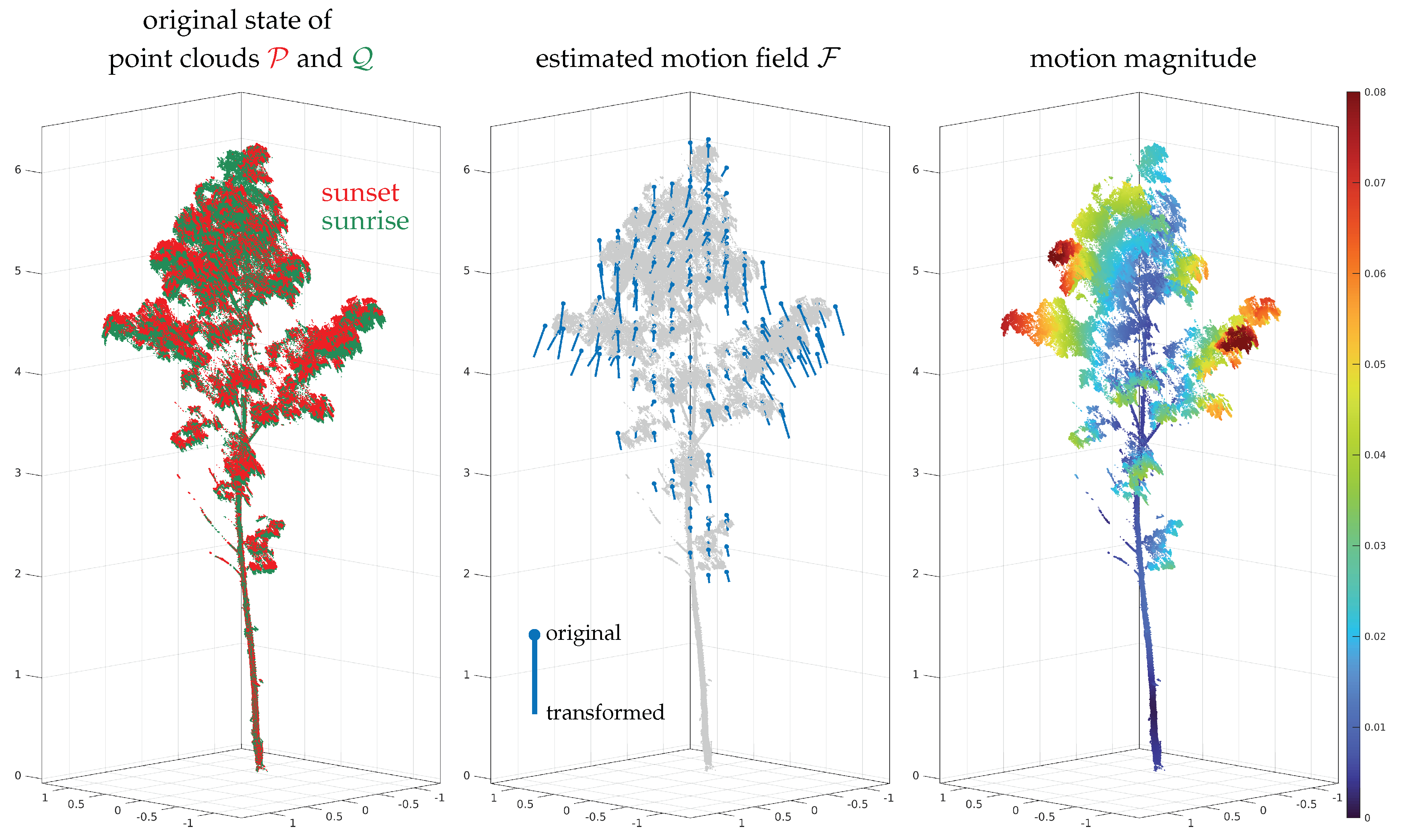
Figure 2.
ICP-based point cloud registration pipeline.
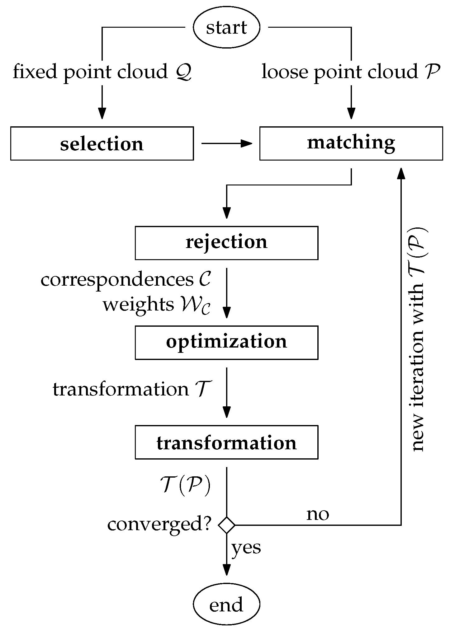
Figure 3.
Typical systematic georeferencing errors of airborne laser scanning (ALS) point clouds (b–d) and their superposition (e). Without access to the trajectory and lidar data, such an error pattern can only be corrected by means of a non-rigid transformation.
Figure 3.
Typical systematic georeferencing errors of airborne laser scanning (ALS) point clouds (b–d) and their superposition (e). Without access to the trajectory and lidar data, such an error pattern can only be corrected by means of a non-rigid transformation.
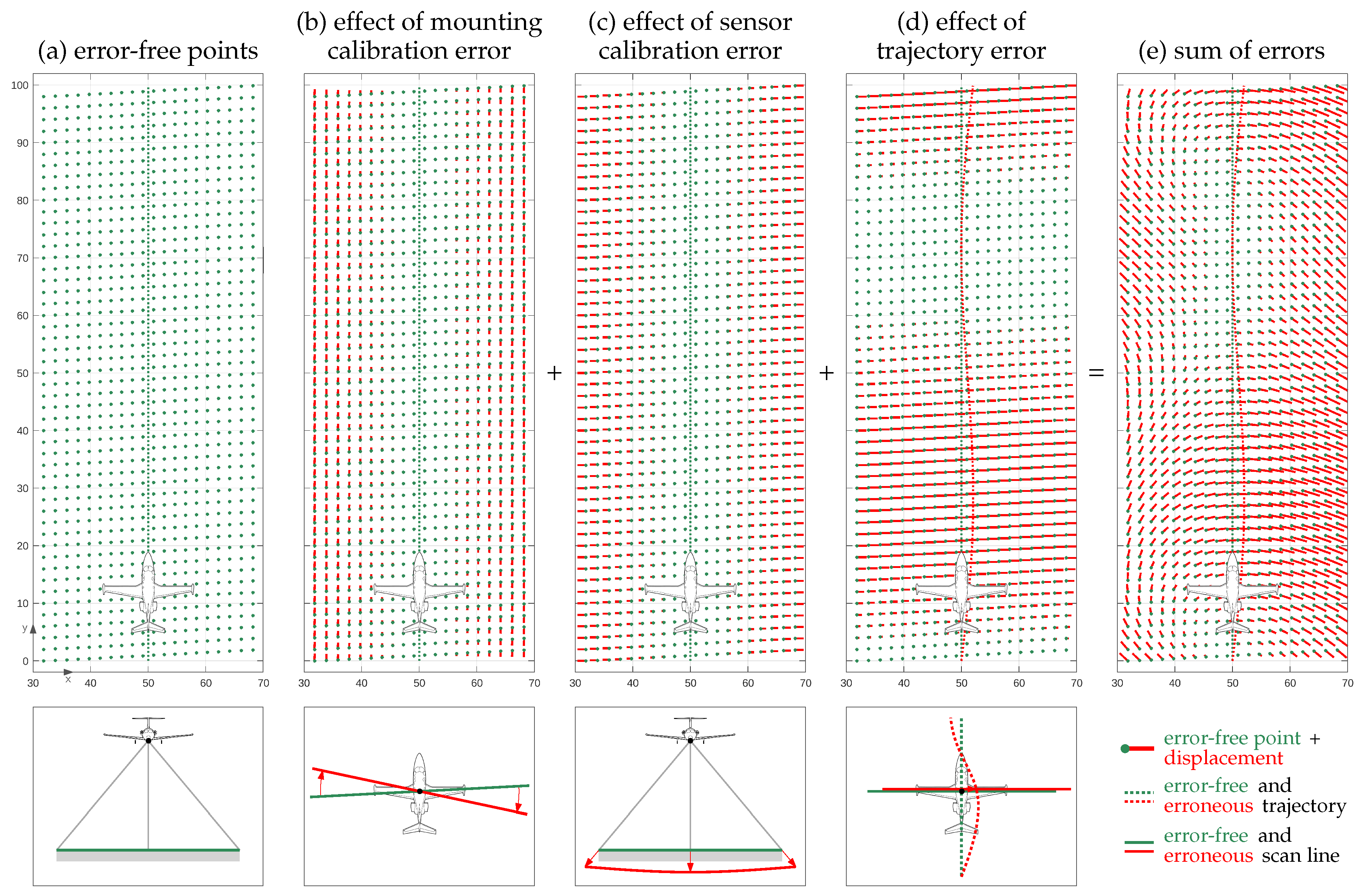
Figure 4.
Example of a 2D transformation field with graph-based control structure, linear interpolation as continuity model, and rigid-body transformation as local transformation model. The white area corresponds to the domain of .
Figure 4.
Example of a 2D transformation field with graph-based control structure, linear interpolation as continuity model, and rigid-body transformation as local transformation model. The white area corresponds to the domain of .
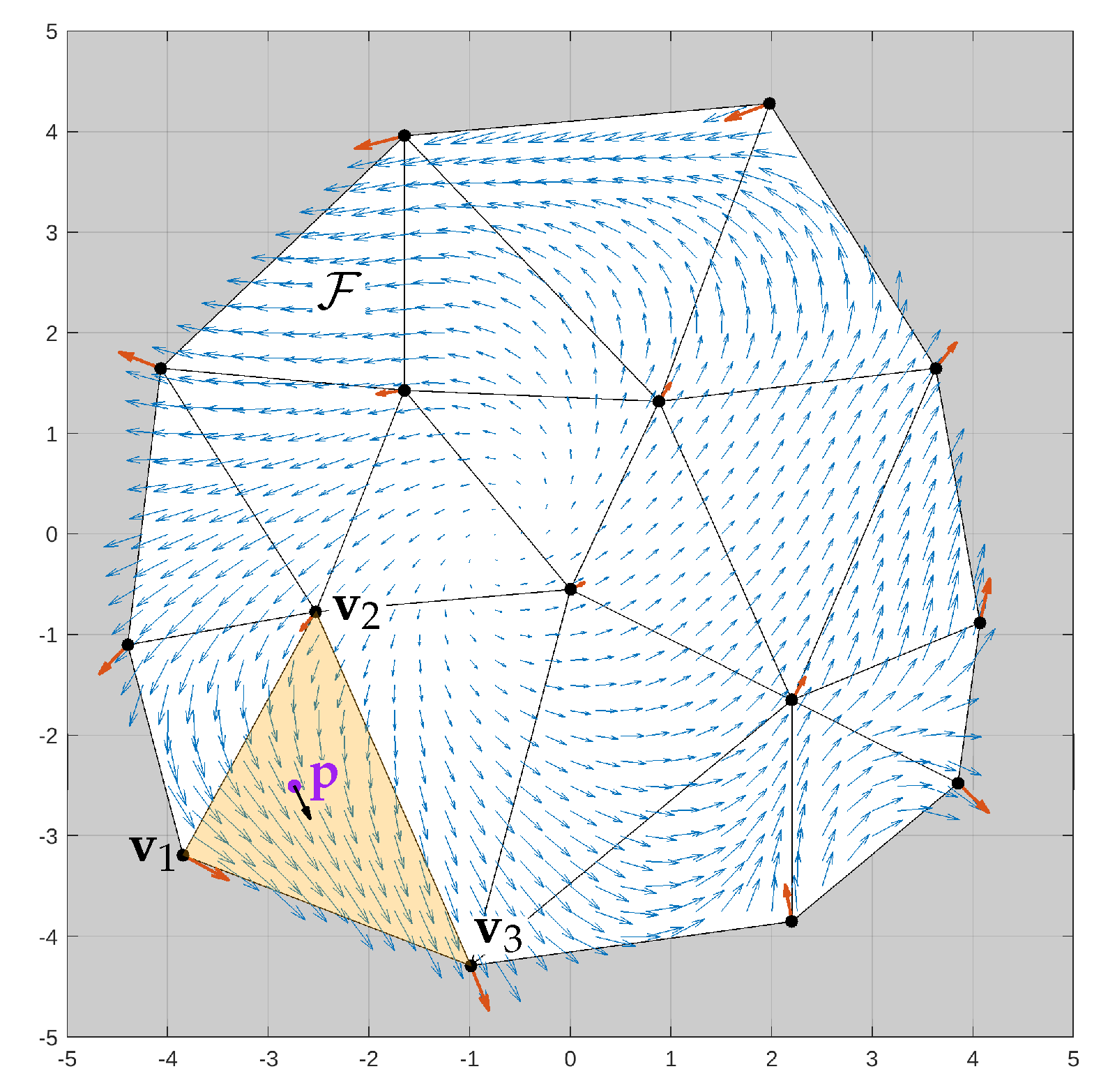
Figure 5.
Types of control structures for transformation fields.
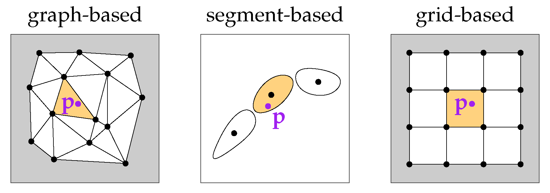
Figure 6.
The non-rigid transformation is modelled by piece-wise tricubic polynomials in a voxel structure; TFCS = transformation field coordinate system (e.g. UTM), VCS = voxel coordinate system.
Figure 6.
The non-rigid transformation is modelled by piece-wise tricubic polynomials in a voxel structure; TFCS = transformation field coordinate system (e.g. UTM), VCS = voxel coordinate system.
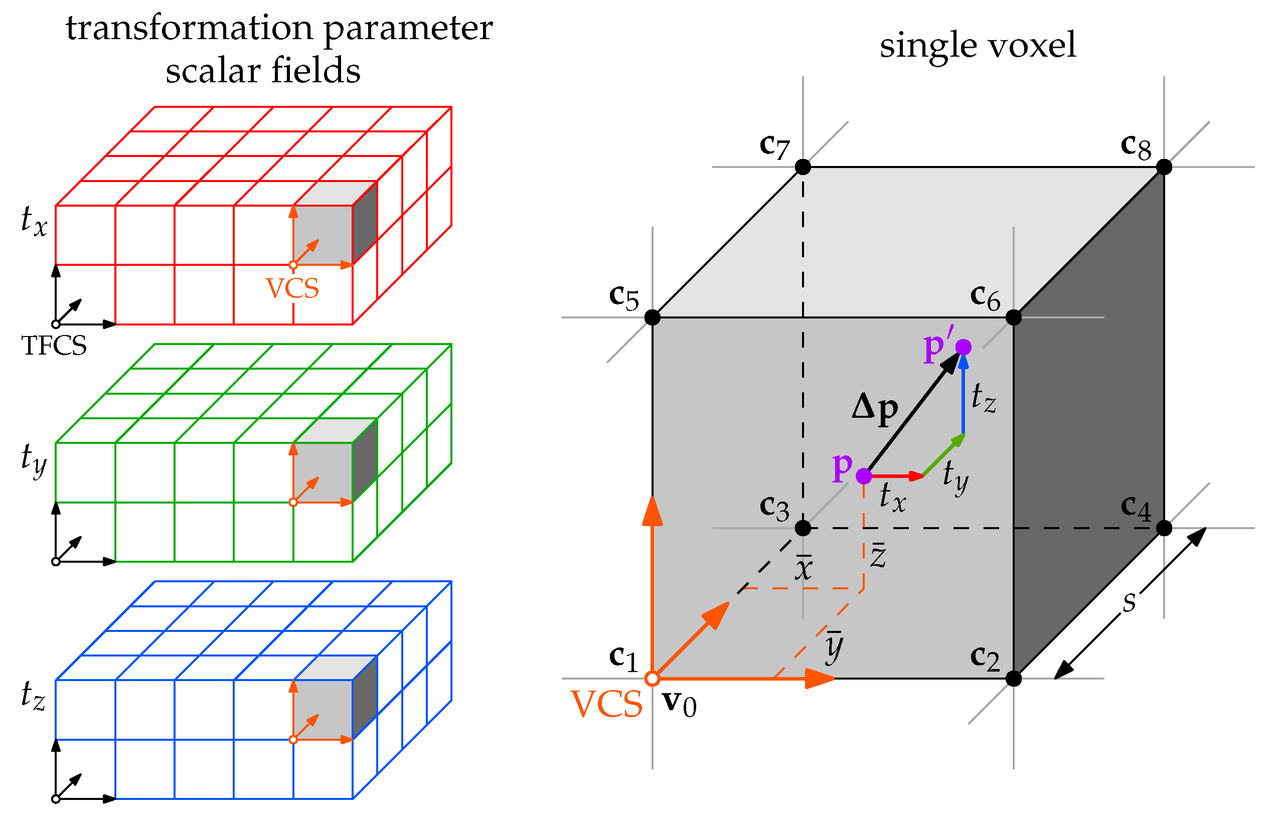
Figure 7.
Example of non-rigid registration of two synthetic point clouds. Red: loose point cloud . Green: fixed point cloud . Correspondences between and are visualized as lines in the upper left image. The transformation field is visualized as vector field in the upper right image.
Figure 7.
Example of non-rigid registration of two synthetic point clouds. Red: loose point cloud . Green: fixed point cloud . Correspondences between and are visualized as lines in the upper left image. The transformation field is visualized as vector field in the upper right image.
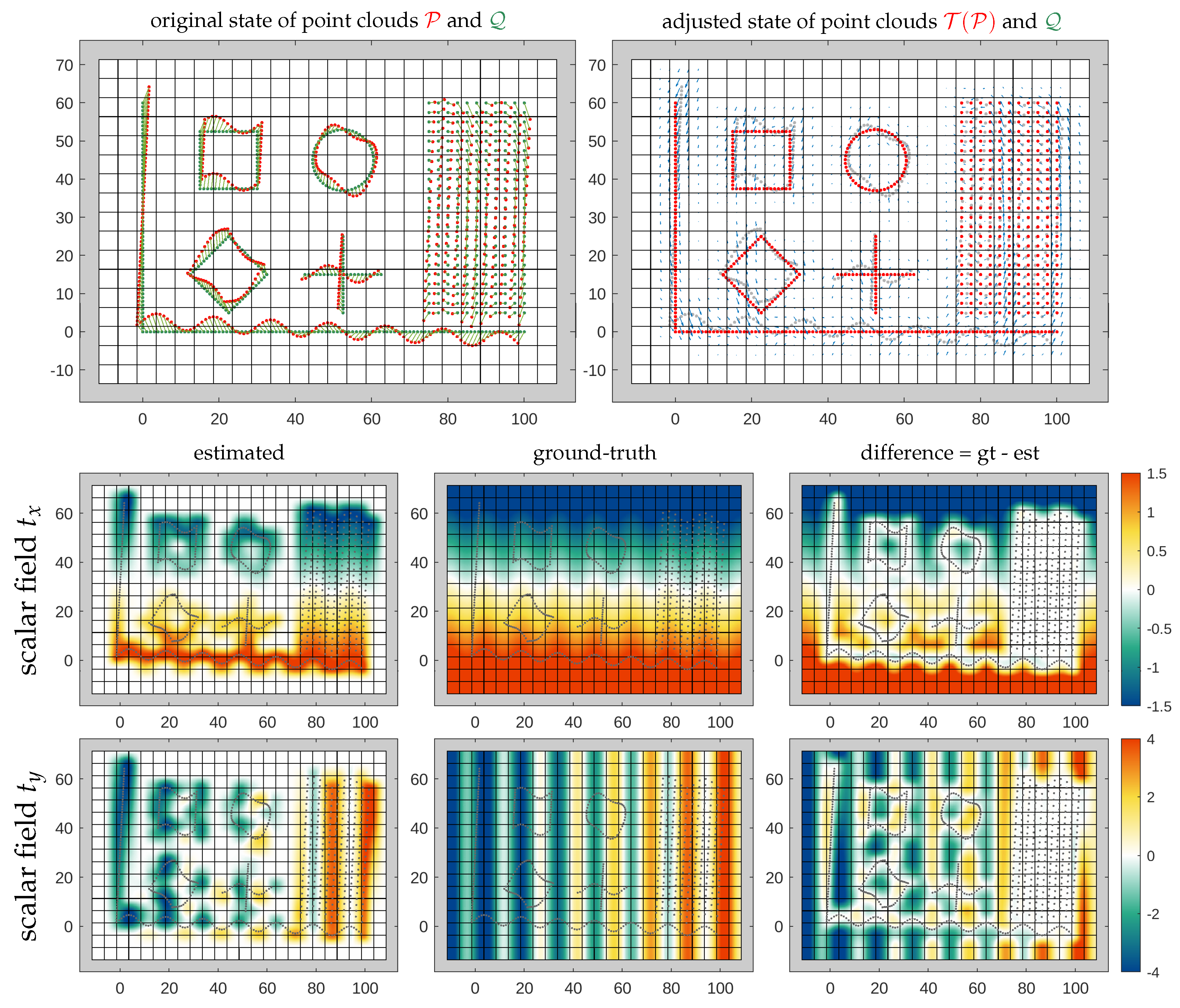
Figure 8.
Effect of varying the weights and of the regularizing observations on the estimated scalar fields and ; GoF = goodness-of-fit, C = condition number.
Figure 8.
Effect of varying the weights and of the regularizing observations on the estimated scalar fields and ; GoF = goodness-of-fit, C = condition number.
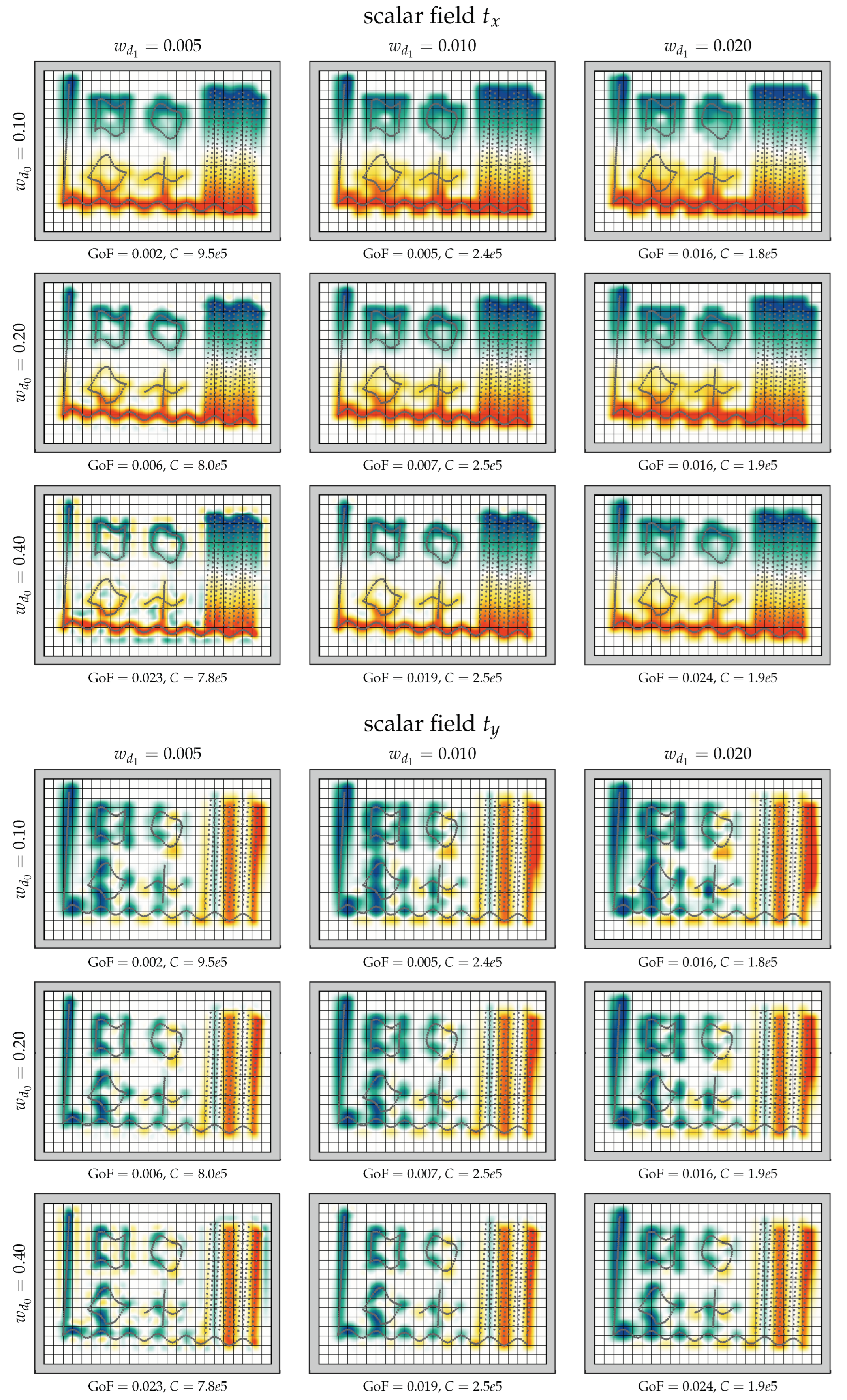
Figure 9.
Effect of different cell sizes on the estimated scalar fields and ; GoF = goodness-of-fit, C = condition number.
Figure 9.
Effect of different cell sizes on the estimated scalar fields and ; GoF = goodness-of-fit, C = condition number.
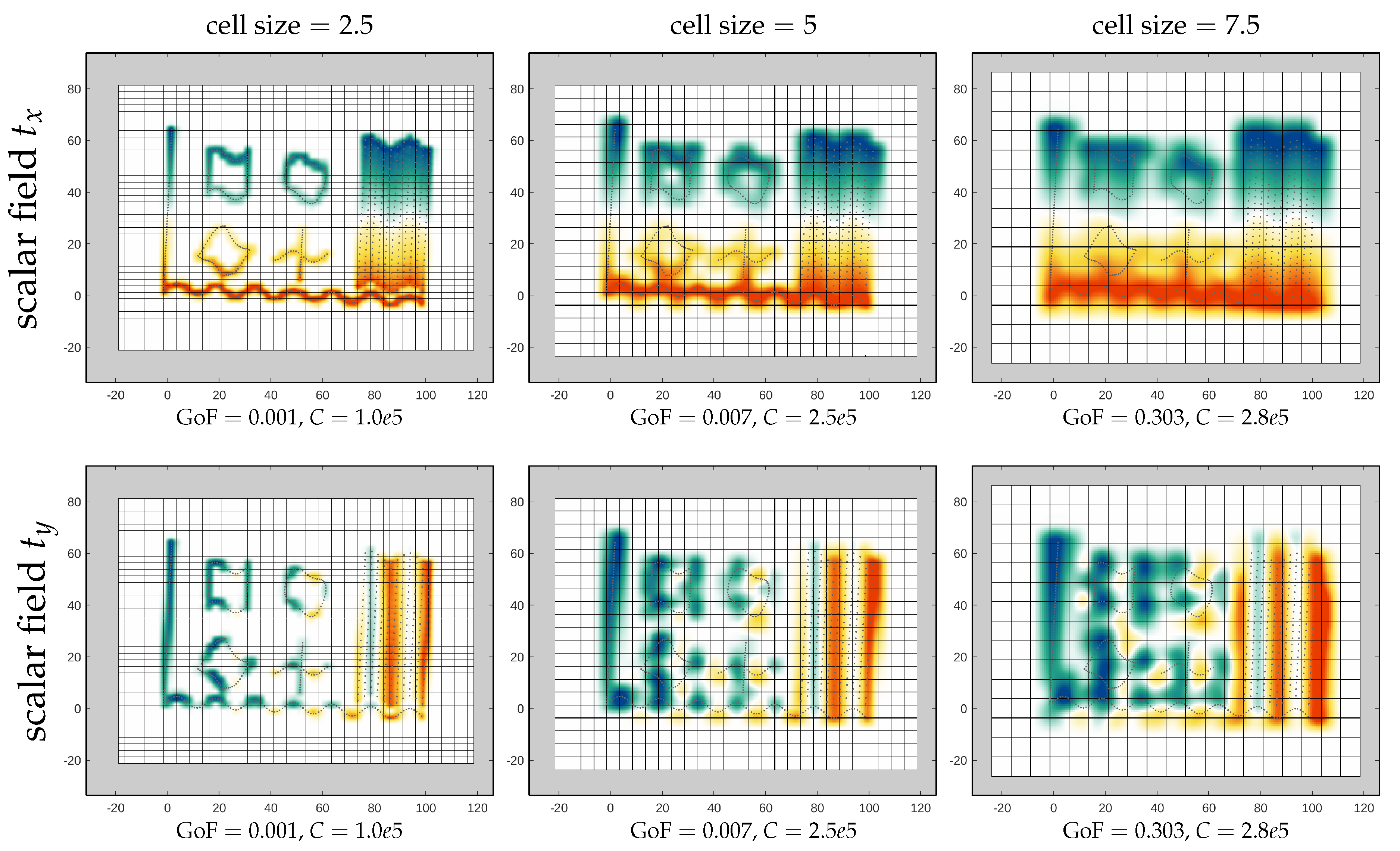
Figure 10.
Open source implementation of our method for two-dimensional point clouds – it can be downloaded here. The depicted example corresponds to the right column in Figure 9.
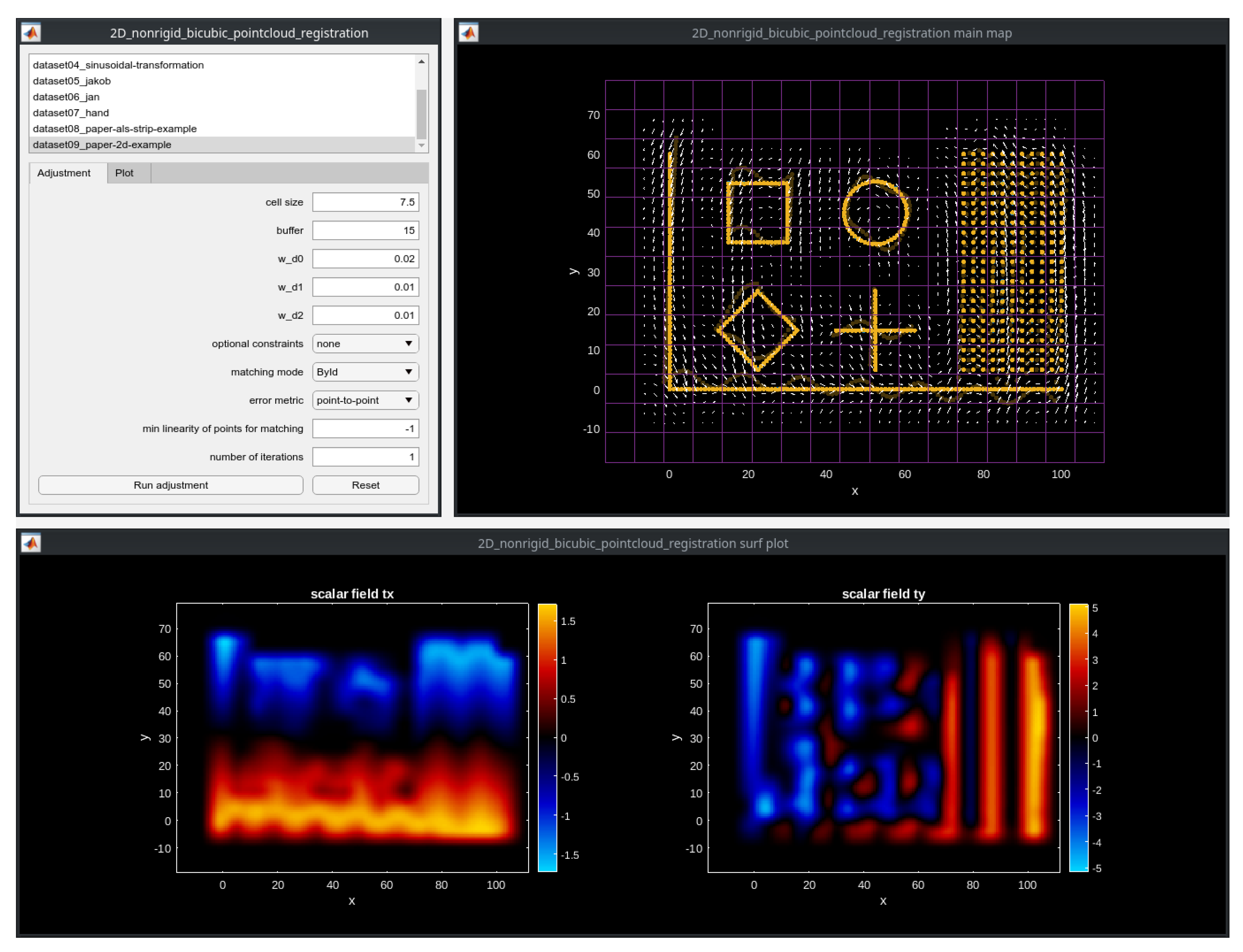
Figure 11.
Improvement of the alignment between two DSMs from 2007 and 2015. The height differences show the errors before (original state) and after (adjusted state) the application of our method. The three images on the right show the estimated shifts in the x, y, and z direction for point cloud . All units in meter.
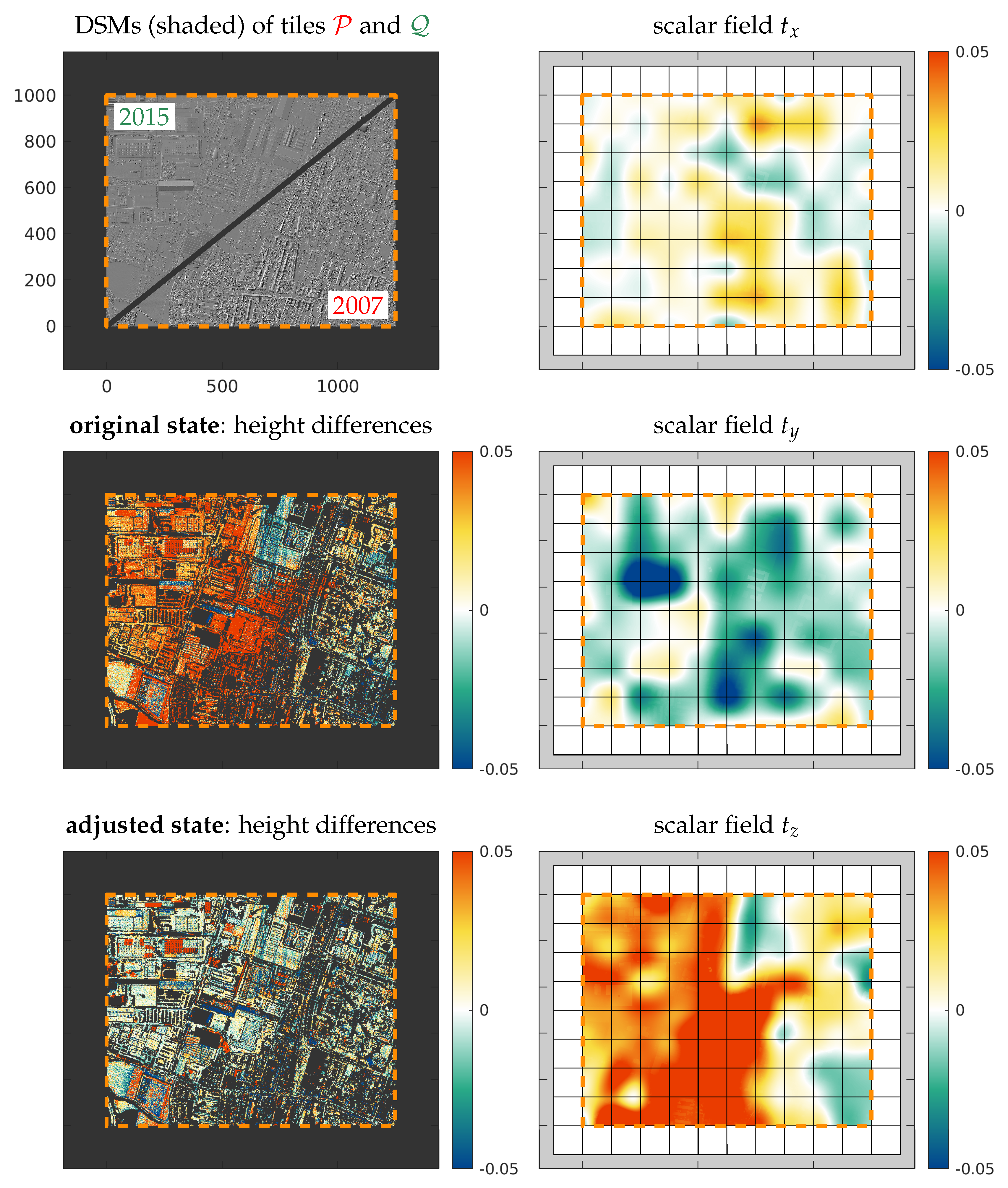
Figure 12.
Improvement of the alignment of two ALS strips. As in the previous example, the height differences show the errors before (original state) and after (adjusted state) the application of our method. The lower three images show the estimated shifts in the x, y, and z direction for point cloud . All units in meter.
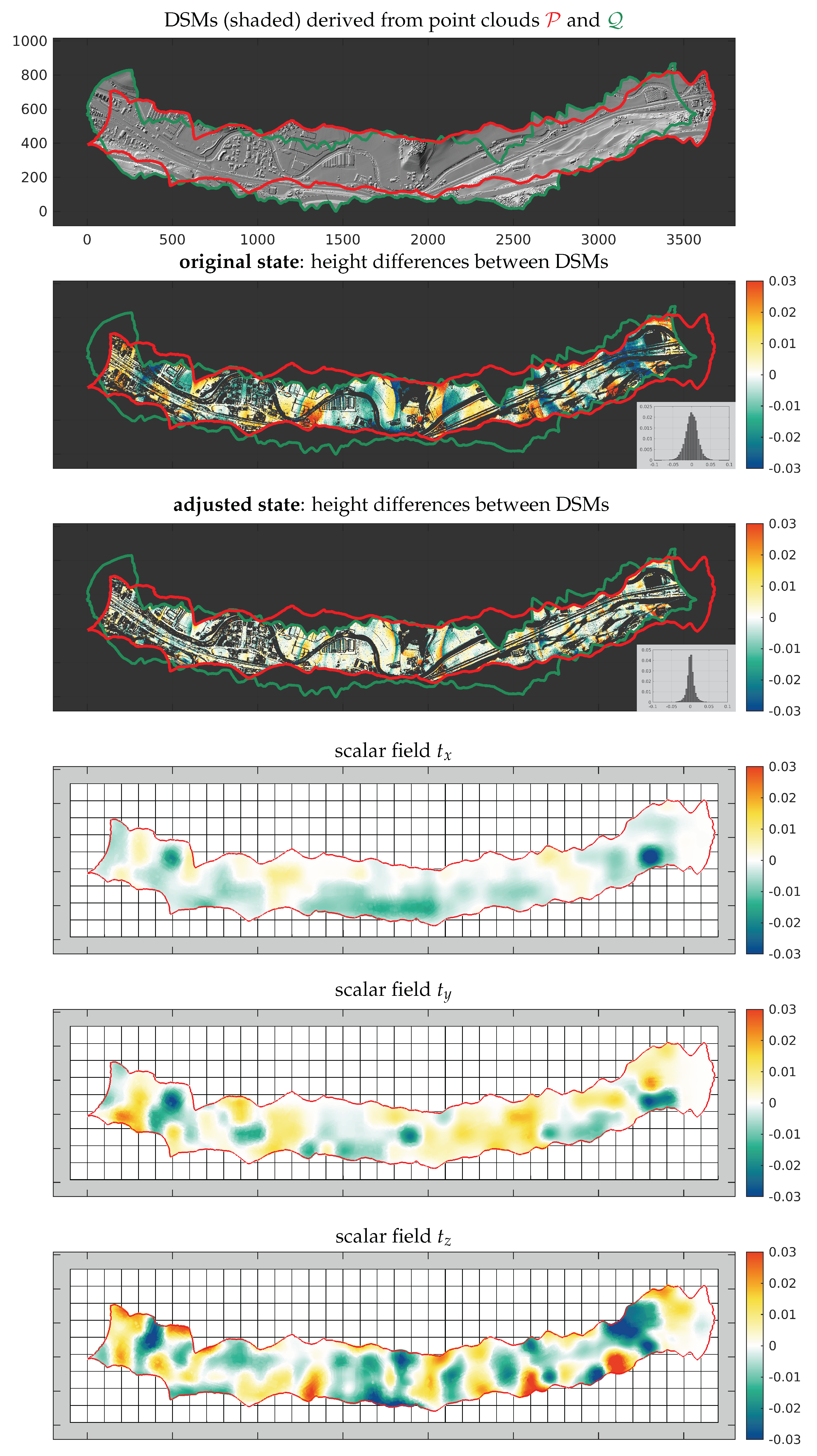
Figure 13.
Improvement of alignment of two MLS strips. Only smooth areas like roads and facades are considered during the registration process. The images on the right show the alignment error between the two point clouds in their original state (top), after adjustment with a 6DoF-ICP (middle) and after our method (bottom). All units in meter.
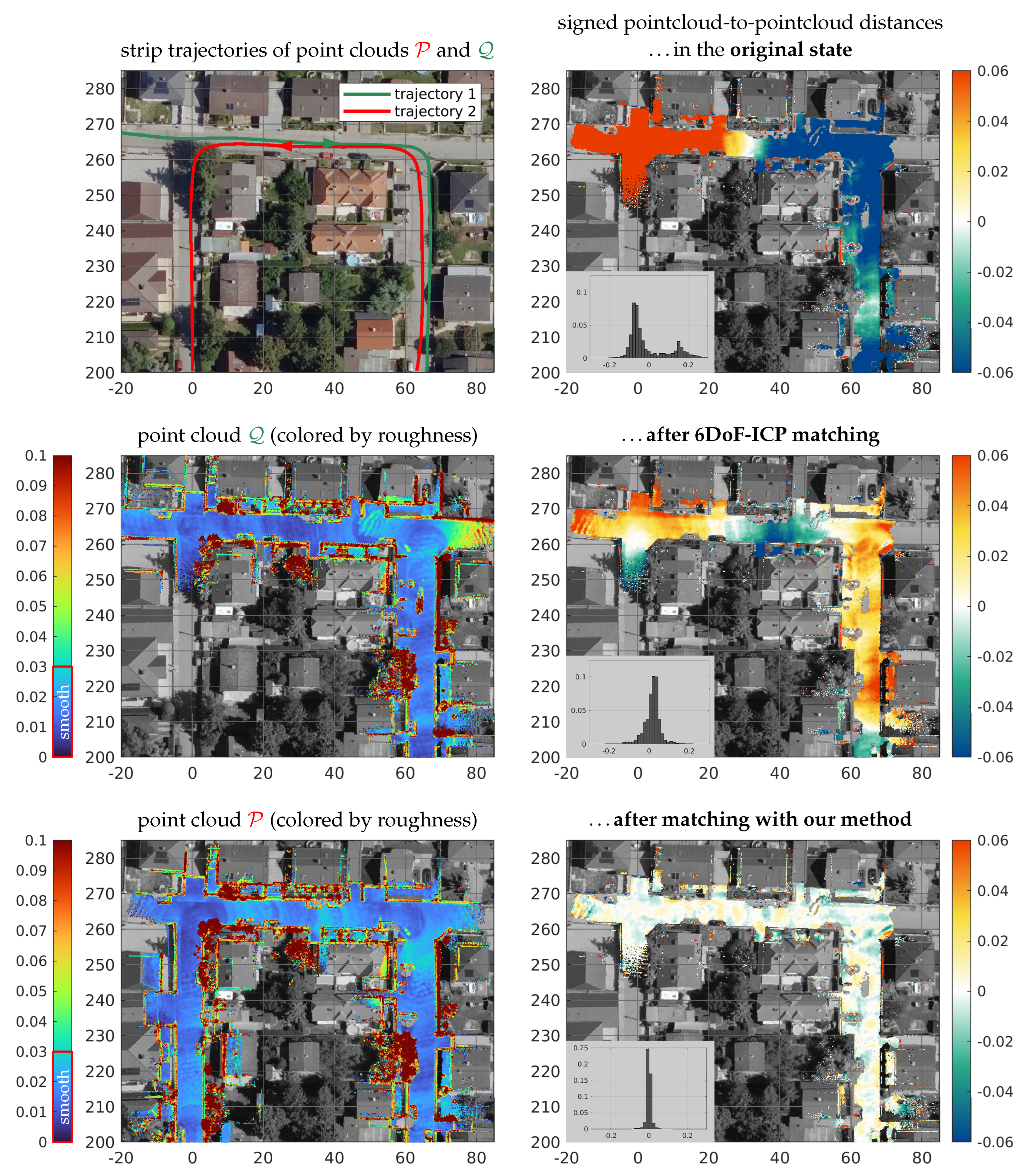
Figure 14.
Estimation of a dense optical flow between two images.
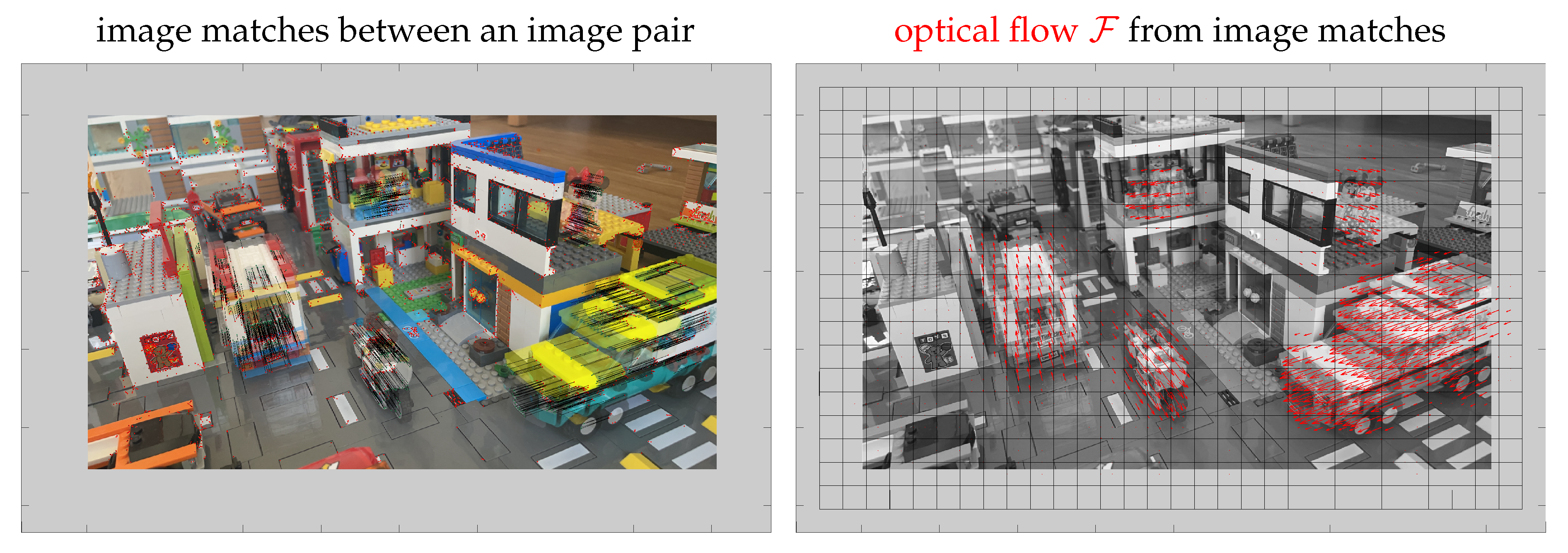
Figure 15.
Non-rigid registration of two point clouds from [18].
Figure 15.
Non-rigid registration of two point clouds from [18].
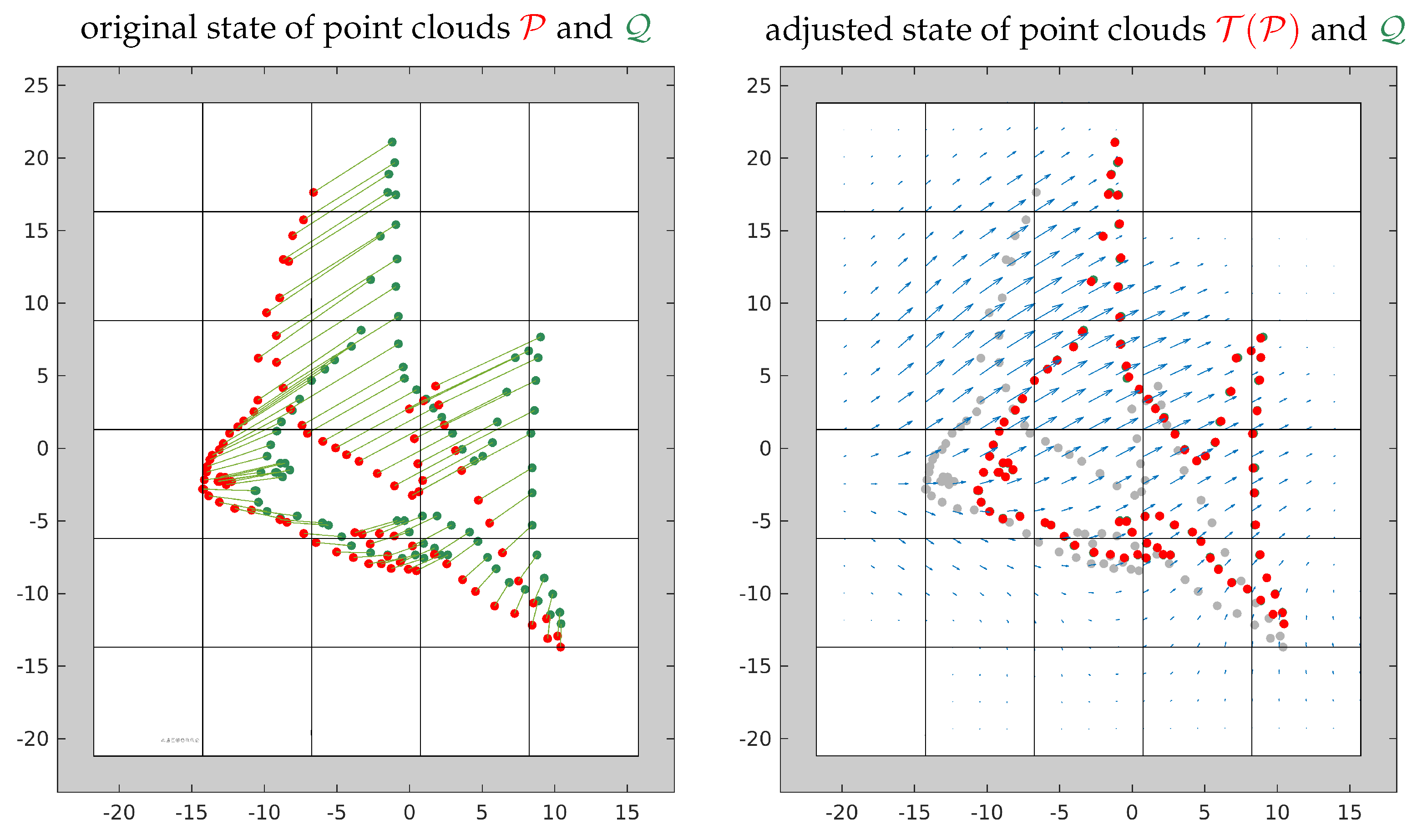
Figure 16.
Non-rigid registration of two hand-shaped point clouds.
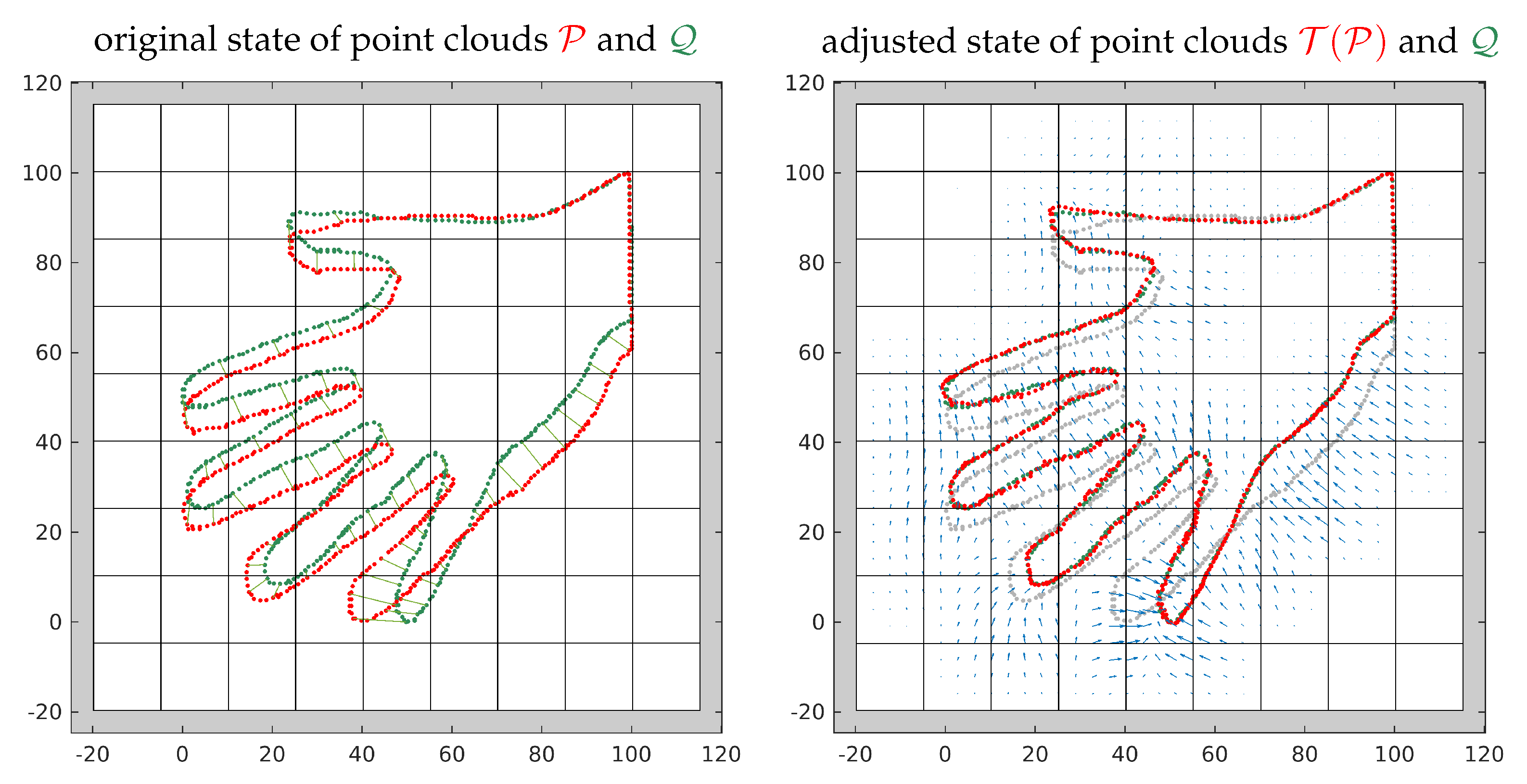
Table 1.
Overview of the datasets used in the experiments and the corresponding input parameter values.
Table 1.
Overview of the datasets used in the experiments and the corresponding input parameter values.
| Experimental results | ||||||||||
|---|---|---|---|---|---|---|---|---|---|---|
| use case | sec. | 2D/3D | cell size | regularization weights | #corresp. | #it. | ||||
| 1 | ALS 1 | Section 6.1 | 3D | 125.0 m | 2.00 | 2.00 | 2.00 | 2.00 | 20000 | 3 |
| 2 | ALS 2 | Section 6.2 | 3D | 100.0 m | 1.00 | 1.00 | 1.00 | 0.10 | 20000 | 3 |
| 3 | MLS | Section 6.3 | 3D | 5.0 m | 0.10 | 0.10 | 0.10 | 0.10 | 10000 | 3 |
| 4 | TLS | Section 6.4 | 3D | 2.0 m | 0.01 | 0.01 | 0.01 | 0.01 | 10000 | 5 |
| 5 | Opt. flow | Section 6.5 | 2D | 15.0 px | 0.20 | 0.10 | 0.10 | – | 6713 | 1 |
| 6 | Fish | Section 6.6 | 2D | 7.5 | 0.10 | 0.10 | 0.10 | – | 91 | 1 |
| 7 | Hand | Section 6.6 | 2D | 15.0 | 0.05 | 0.05 | 0.10 | – | 36 | 1 |
Disclaimer/Publisher’s Note: The statements, opinions and data contained in all publications are solely those of the individual author(s) and contributor(s) and not of MDPI and/or the editor(s). MDPI and/or the editor(s) disclaim responsibility for any injury to people or property resulting from any ideas, methods, instructions or products referred to in the content. |
© 2023 by the authors. Licensee MDPI, Basel, Switzerland. This article is an open access article distributed under the terms and conditions of the Creative Commons Attribution (CC BY) license (http://creativecommons.org/licenses/by/4.0/).
Copyright: This open access article is published under a Creative Commons CC BY 4.0 license, which permit the free download, distribution, and reuse, provided that the author and preprint are cited in any reuse.


