
Submitted:
26 June 2025
Posted:
30 June 2025
You are already at the latest version
Abstract
Point cloud denoising is essential for improving 3D data quality, yet traditional K-means methods relying on Euclidean distance struggle with non-uniform noise. This paper proposes a K-means algorithm leveraging Total Bregman Divergence (TBD) to better model geometric structures on manifolds, enhancing robustness against noise. Specifically, TBDs - Total Logarithm, Exponential, and Inverse Divergences - are defined on symmetric positive-definite matrices, each tailored to capture distinct local geometries. Theoretical analysis demonstrates the bounded sensitivity of TBD-induced means to outliers via influence functions, while anisotropy indices quantify structural variations. Numerical experiments validate the methods superiority over Euclidean-based approaches, showing effective noise separation and improved stability. The work bridges geometric insights with practical clustering, offering a robust framework for point cloud preprocessing in vision and robotics applications.
Keywords:
Total Bregman divergence
; point cloud denoising
; K-means clustering
; manifold learning
; influence function
; anisotropic index
1. Introduction
In recent years, the rapid advancement of 3D scanning technologies has led to an explosion of point cloud data in various fields, including computer vision, robotics, and autonomous systems [1,2,3,4]. As raw digitalizations of physical structures, point clouds often contain inherent noise that degrades segmentation and 3D reconstruction fidelity. Despite their utility, raw point cloud datasets frequently contain inherent imperfections like noise and outliers that compromise the accuracy of downstream applications including segmentation and 3D reconstruction. This inherent data quality challenge necessitates robust denoising algorithms as a fundamental preprocessing requirement for reliable 3D analysis [5,6,7,8,9,10].
Among the various denoising techniques, clustering-based methods have shown promising results due to their ability to group similar points together and distinguish between signal and noise [11,12]. While conventional K-means clustering demonstrates effectiveness in regular data spaces, its dependence on isotropic distance measures creates fundamental limitations when processing irregular 3D structures. Specifically, the Euclidean metric fails to adequately characterize manifold geometries inherent to point cloud data, particularly under spatially variant noise conditions.
Our methodological contribution resolves this through a density-aware clustering framework that adapts to local topological characteristics [13,14]. Given the differences in local geometric structures between noise and valid data on the manifold, points with similar local features should be grouped together into the same cluster. Previous studies [15,16] have employed the K-means clustering algorithm for point cloud denoising, but they relied solely on a limited number of metrics to measure distances on the manifold. Furthermore, these studies overlooked the influence function, which is crucial for evaluating the robustness of the mean derived from each metric in the presence of outliers. Conversely, [17] proposed a point cloud denoising method leveraging the geometric structure of the Gaussian distribution manifold, employing five distinct measures: Euclidean distance, Affine-Invariant Riemannian Metric (AIRM), Log-Euclidean Metric (LEM), Kullback-Leibler Divergence (KLD), and its symmetric variant (SKLD). The research evaluated metric robustness by deriving influence functions for mean estimators under outlier conditions. Experimental results revealed that geometric metrics outperformed Euclidean measurements in denoising quality, with geometric means showing greater outlier resistance than arithmetic means. Notably, KLD and SKLD demonstrated computational advantages over AIRM/LEM through reduced complexity. Bregman divergence extends squared Euclidean distances to diverse data-adaptive metrics, enabling more efficient computation of means and influence functions compared to AIRM/LEM frameworks, thus enhancing processing efficiency while maintaining theoretical rigor.
This work introduces a novel divergence class measuring orthogonal deviation between a convex differentiable function’s value at one point and its tangent approximation at another, formally termed Total Bregman Divergence (TBD). A schematic comparison in [18] visually clarifies TBD’s geometric distinction from conventional Bregman divergence. Notably, the Total Bregman Divergence exhibits heightened robustness and adaptability when managing intricate data structures.
This paper builds upon our previous concept presented in [17] by introducing a novel class of methods specifically designed for point cloud denoising. Furthermore, we implement the idea of K-means clustering, leveraging local statistical features to distinguish between noise and valid data. TBD offers advantages over traditional Bregman divergence by providing invariance to coordinate transformations, measuring orthogonal distance between function values and tangents, potentially improving robustness against noise, and generalizing the standard Bregman divergence while retaining its useful properties, albeit the specific benefits may vary depending on the application context and function choice.
Three fundamental breakthroughs constitute the core innovations of this research:
(1) We introduce a K-means clustering algorithm based on TBDs specifically designed for denoising high-density noise point clouds. This methodology capitalizes on the local statistical differences between noise and valid data within the context of Gaussian distribution families.
(2) Bregman divergences are defined on the manifold of positive definite matrices by employing convex functions. Associated with these divergences, anisotropic indices are proposed, which serve to reflect the local geometric structure surrounding each point on the matrix manifold. Furthermore, TBDs are endowed on the manifold, including the total logarithm divergence (TLD), the total exponent divergence (TED), and the total inverse divergence (TID).
(3) The means of several positive-definite matrices are computed based on TBDs. To evaluate the robustness of these means, approximations and upper bounds for their influence functions are provided. Numerical simulations reveal that the loss function of the TBDs-induced means is lower than that induced by the Euclidean distance, and the weighted logarithm Euclidean divergence exhibits a smaller cost function compared to the mean induced by the logarithmic Euclidean metric, thereby affirming the algorithm’s effectiveness and advantage.
The paper is structured into six main sections. Section 1 introduces the importance of point cloud denoising and highlights the limitations of traditional K-means clustering approaches based on Euclidean distance. Section 2 delves into the theoretical foundations, defining TBD and deriving the means of several positive-definite matrices. Section 3 proposes a novel K-means clustering algorithm that leverages TBD for point cloud denoising. Section 4 provides an in-depth analysis of the anisotropy indices of Bregman divergence and the influence functions of the TBD means. Section 5 presents simulation results and performance comparisons, demonstrating the effectiveness of the proposed algorithm. Section 6 concludes by summarizing the main contributions and discussing potential applications and future research directions.
2. Geometry on the Manifold of Symmetric Positive-Definite Matrices
The collection of real matrices is represented by , whereas the subset comprising all invertible real matrices forms the general linear group, denoted as . Notably, possesses a differentiable manifold structure, with functioning as its Lie algebra, denoted as . The exchange of information between and is facilitated by exponential and logarithmic mappings. In particular, the exponential map, given by
converts a matrix X in to an element in . Conversely, for an invertible matrix A devoid of eigenvalues on the closed negative real axis, there exists a unique logarithm with eigenvalues within the strip . This logarithm, serving as the inverse of the exponential map, is termed the principal logarithm map and symbolized by
Let denote the space of real symmetric matrices:
The subset of symmetric positive-definite matrices forms the Riemannian manifold:
Three fundamental metric structures on are considered:
- (i)
-
Euclidean (Frobenius) Framework: The canonical inner product on is defined asinducing the norm and metric distanceThe tangent space at any coincides with due to ’s open submanifold structure in .
- (ii)
-
Affine-Invariant Riemannian Metric (AIRM): The geometry metric at is given by
- (iii)
-
Log-Euclidean Metric (LEM): Through the logarithmic group operationbecomes a Lie group. The metric at is defined via differential mappings:
where denotes the differential of the matrix logarithm. The corresponding distance becomes
effectively Euclideanizing the manifold geometry through logarithmic coordinates.
2.1. Bregman Divergence on Manifold
For matrices , the Bregman matrix divergence associated with a strictly convex differentiable potential function is given by:
where denotes the Frobenius inner product [21].
This divergence can be systematically extended to a total Bregman divergence (TBD) through the subsequent formulation. For invertible matrices , the TBD is defined as [22]
When calculating the divergence associated with a certain convex function , the Riemannian gradient of is often needed, which can be obtained by the covariant/directional derivative related to the Riemannian metric as follows:
with the curve and . After linearizing the curve , (12) can be rewritten as
Proposition 1.
For any nonsingular matrix with spectral exclusion condition , there exists a well-defined matrix entropy functional:
which generalizes the scalar function to the matrix setting through trace-theoretic extension [22]. Then, the Riemannian gradient of is
Furthermore, the Bregman divergence is expressed as follows
and the total logarithm divergence (TLD) is provided by
Proof.
Similar to the proof methodology employed in Proposition 1, we can derive Proposition 2 and Proposition 3 through analogous applications.
Proposition 2.
Consider which is induced from the function [21]. Then, the Riemannian gradient of is
Furthermore, the Bregman divergence is expressed as
and the total exponential divergence (TED) is provided by
Proposition 3.
When A is invertible and let , which is induced from the function [21]. Then, the Riemannian gradient of is
Furthermore, the Bregman divergence is expressed as follows
and the total inverse divergence (TID) is provided by
To analyze the differences among the TBD divergences defined on the positive-definite matrix manifold, Figure 1 shows 3-dimensional isosurfaces centered at the identity matrix, which are induced by TLD, TED, and TID, respectively. All of these isosurfaces are convex balls with non-spherical shapes, differing completely from the spherical isosurfaces in the context of the Euclidean metric.
2.2. TBDs Means on
In this subsection, we study the geometric mean of several symmetric positive-definite matrices induced by the TBD, by considering the minimization problem of an objective function.
For m positive real numbers , the arithmetic mean is often denoted as and expressed as
where represents the absolute difference between a and , which signifies the distance separating the two points on the real number line. The mean of m symmetric positive-definite matrices is the solution to
Thus, the arithmetic mean of endowed by the Euclidean metric can be represented as
And, the mean of with LEM is [16]
The result indicates that the Log-Euclidean mean has Euclidean characteristics when considered in the logarithmic domain, whereas AIRM’s mean lacks these properties [17].
The concept extends naturally to the TBD mean. For a strictly convex differentiable function and matrices , the TBD mean is defined as
The strict convexity of ensures the Bregman divergence retains strict convexity in A. Consequently, uniqueness of the TBD mean (30) follows directly from convex optimization principles, provided such a mean exists. To guarantee existence, must operate within a compact subset of the symmetric positive-definite matrix manifold . Compactness ensures adherence to the Weierstrass extreme value theorem, which mandates attainment of minima for continuous functions over closed and bounded domains conditions inherently satisfied by the convex functional on this Riemannian manifold. Let’s define as
According to (13), the Riemannian gradient of can be obtained as
Then, by solving , the TBD mean can be expressed as
with the weight
Next, by substituting (15), (20), and (23) into (33) respectively, it is straightforward to get explicit expressions for the means corresponding to TLD, TED, and TID.
Proposition 4.
The TLD mean of m symmetric positive-definite matrices is provided by
where
By comparing (29) and (35), it can be seen that the TLD mean is essentially a weighted version of the LEM mean.
Proposition 5.
The TED mean of m symmetric positive-definite matrices is provided by
where
Proposition 6.
The TID mean of m positive definite matrices is provided by
where
3. K-Means Clustering Algorithm with TBDs
In the n-dimensional Euclidean space , we denote a point cloud of size as
For , we first identify its local neighborhood using the k-nearest neighbors algorithm. Subsequently, the intrinsic geometry of is characterized by computing two statistical descriptors:
1. The centered mean vector:
where denotes empirical expectation;
2. The covariance operator:
quantifying pairwise positional deviations.
These descriptors induce a parameterization of as points on the statistical manifold of n-dimensional Gaussian distributions
where f denotes the probability density function. This geometric embedding facilitates subsequent analysis within the framework of information geometry. The point cloud undergoes local statistical encoding through operator , generating its parametric representation in symmetric matrix space. This mapped ensemble, termed the statistical parameter point cloud, preserves neighborhood geometry through covariance descriptors while enabling manifold-coordinate analysis.
Due to the topological homeomorphism between and [23], the geometric structure on can be induced by assigning metrics on . Additionally, the distance on is denoted as
where stands for the difference between and . The mean of on the parameter point cloud is denoted as , where
The definitions of both distance and mean operators on are contingent upon the specific metric structure imposed on . In our proposed algorithm, these fundamental statistical measures will be directly computed through TBDs, which play a crucial role in establishing the geometric framework for subsequent computations.
The intrinsic statistical properties of valid and stochastic noise components exhibit fundamental divergences in their local structural organizations. This statistical separation forms the basis for our implementation of a K-means clustering framework to partition the complete dataset into distinct phenomenological categories: structured information carriers and unstructured random perturbations. The formal procedure for this discriminative clustering operation is systematically outlined in Algorithm 1.
| Algorithm 1 Signal-Noise Discriminative Clustering Framework. |
|
4. Anisotropy Index and Influence Functions
This chapter establishes a unified analytical framework for evaluating geometric sensitivity and algorithmic robustness on . Section 4.1 introduces the anisotropy index as a key geometric descriptor, formally defining its relationship with fundamental metrics including the Euclidean metric, AIRM, and the Bregman divergences. Through variational optimization, we derive closed-form expressions for these indices, revealing their intrinsic connections to matrix spectral properties. Section 4.2 advances robustness analysis through the influence function theory, developing perturbation models for three central tensor means: TLD, TED, and TID. By quantifying sensitivity bounds under outlier contamination, we establish theoretical guarantees for each mean operator.
4.1. The Anisotropy Index Related to Some Metrics
The discriminatory capacity of weighted positive definite matrices manifests through their associated anisotropy measures. Defined intrinsically on the matrix manifold , the anisotropy index quantifies local geometric distortion relative to isotropic configurations. For , the anisotropy measure relative to the Riemannian metric is
This index corresponds to the squared minimal projection distance from A to the scalar curvature subspace . Larger values indicate stronger anisotropic characteristics. For explicit computation, we minimize the metric-specific functional:
Next, we systematically investigate anisotropy indices induced by three fundamental geometries: the Frobenius metric representing Euclidean structure, AIRM characterizing curved manifold topology, and Bregman divergences rooted in information geometry. This trichotomy reveals how metric selection governs directional sensitivity analysis on the symmetric positive-definite matrix manifold.
Following Equations (3) and (45), the anisotropy index associated with the Euclidean metric can be derived through direct computation.
Proposition 7.
Proposition 8.
The anisotropy index associated with AIRM at a point is formulated as
where
Proof.
Proposition 9.
Proposition 10.
Proposition 11.
4.2. Influence Functions
This subsection develops a robustness analysis framework through influence functions for symmetric positive-definite matrix-valued data. We systematically quantify the susceptibility of the TBD mean estimators under outlier contamination by deriving closed-form expressions of influence functions. Furthermore, we establish operator norm bounds of influence functions, thereby characterizing their stability margins in perturbed manifold learning scenarios.
Let denote the TBDs mean of m symmetry positive-definite matrices . Let denote the mean after adding a set of l outliers with a weight to [25,26]. Therefore, can be defined as follows:
which shows that is a perturbation of and is defined as the influence function. Let denote the objective function to be minimized over the symmetric positive-definite matrices, formulated as follows:
Given that denotes the mean of symmetric positive-definite matrices, the optimality condition requires , which gives:
By taking the derivative of the equation with respect to and evaluating it at , we obtain
Next, the influence functions of TLD mean, TED mean, and TID mean are given by the following properties.
Proposition 12.
TLD mean of m symmetry positive-definite matrices and l outliers is with
Furthermore,
Proof.
Following from (15), we derive
Then, substituting (74) into (71) and computing the trace on both sides, we obtain
By considering the arbitrariness of , we derive (72) for the TLD mean. Furthermore, it can be deduced that the influence function has an upper bound (73), and is independent of outliers . □
Proposition 13.
TED mean of m symmetric positive-definite matrices and l outliers is , where
Furthermore,
Proof.
Following from (20), we derive
Then, substituting (78) into (71) and computing the trace on both sides, we obtain
By considering the arbitrariness of , we derive (76) for the TED mean. Furthermore, it can be deduced that the influence function has an upper bound (77), and is independent of outliers . □
Proposition 14.
TID mean of m symmetry positive-definite matrices and n outliers is , where
Furthermore,
Proof.
Following from (23), we derive
Then, substituting (82) into (71) and computing the trace on both sides, we obtain
By considering the arbitrariness of , we get (80) for the TED mean. Furthermore, it can be deduced that the influence function has an upper bound (81), and is independent of outliers . □
While the influence function of the AIRM Mean demonstrates unboundedness with respect to its input matrices [24], all of the TBD means exhibit bounded influence functions under equivalent conditions.
5. Simulations and Analysis
In the following simulations, the symmetric positive-definite matrices used in Algorithm 1 are generated by
where is a square matrix randomly generated by MATLAB.
A. Simulations and Results
In this example, we apply Algorithm 1 to denoise the point cloud of a teapot, employing TLD as the distance metric. The signal-to-noise ratio (SNR) is specified as 4137:1000, with parameters and . The experiments utilize MATLAB’s built-in Teapot.ply dataset, a standard PLY-format 3D point cloud that serves as a benchmark resource for validating graphics processing algorithms and visualization techniques. To optimize indicator weights and enhance data visualization, we utilize Principal Component Analysis to provide a holistic view of the covariance matrix encompassing all data. Figure 2 (a) displays the initial distribution of valid data and noise prior to denoising. Following that, Figure 2 (b) exhibits the transformed data distribution after applying TLD for denoising. Figure 2 (c) and (d) respectively show the results before and after denoising the teapot. In these figures, blue dots signify noise data, whereas green dots indicate valid data. Figure 2 demonstrates that Algorithm 1 effectively partitions data points into two discrete clusters, achieving explicit separation between valid signals and noise components.
B. Analysis of TBDs Mean Stability
In Figure 3, for the 10 sample data randomly generated by (84) when , we use 100 experiments to compare the loss functions of the means for the Euclidean metrc, TLD, TED, and TID. It is shown that the loss function of the mean for the Euclidean distance is much larger than those of the TBDs. Among the TBDs, the loss function of the TED mean is slightly larger than those of the TLD and TID means. A more minor loss function generally indicates that the algorithm is more stable during the training process, less prone to issues such as gradient explosion or vanishing gradients. This aids the algorithm in finding a better solution within a limited time. Therefore, this indicates that on , the means induced by TLD, TED, and TID are more suitable than those induced by the Euclidean metric.
From (29) and (35), it is shown that the TLD mean is essentially a weighted version of the LEM. Figure 4 compares the loss functions of the TLD mean and that of the LEM mean based on 100 repeated trials conducted on 50 samples generated using (84). As shown in Figure 4, the loss function of the TLD mean is significantly smaller compared to that of the LEM mean. Therefore, by assigning different weights to the elements of the matrix, the weighted mean further reduces the loss function. In practical applications such as image processing, signal analysis, and machine learning, using the weighted mean can be a valuable tool for achieving more accurate and efficient data processing and analysis.
Table 1 benchmarks the denoising performance of Algorithm 1 across four metrics (Euclid, TLD, TED, TID), evaluated through True Positive Rate (TPR), False Positive Rate (FPR), and Signal-to-Noise Ratio Growth (SNRG) under three degradation levels (SNR=10/2/1). At SNR=10, all algorithms hit 100% TPR, but Euclid’s FPR (80.24%) is highest, making it less effective than TLD, TED, and TID. TLD and TED excel in SNRG, with TID leading at 112.82%. As SNR drops to 2, TED stands out with perfect TPR and high SNRG, followed by TLD. TID remains competitive despite TPR decline. Euclid lags in FPR and SNRG. At SNR=1, TED leads in TPR and SNRG, while TID tops FPR and SNRG among all. Euclid fails to match TLD, TED, and TID, especially in FPR minimization and SNRG maximization. In summary, Euclid underperforms TLD, TED, and TID in FPR and SNRG, highlighting their effectiveness in point cloud denoising.
C. Analysis of Computational Complexity
We first analyze the computational complexity of mean operators induced by four metrics: Euclidean, TLD, TED, and TID, mathematically defined in equations (28), (35), (37), and (39). Subsequently, we quantify the computational load for corresponding influence functions, with formulations specified in (72), (76), (80), and Proposition 1 of [17].
Under the framework of m symmetric positive-definite matrices and l outliers, we systematically evaluate computational costs. Considering single-element operations as O(1) and matrix , fundamental operations reveal critical patterns: Matrix inversion and logarithmic operations both require computations. Operations involving matrix exponentials and matrix roots for symmetric positive-definite matrices necessitate eigenvalue decomposition, consequently maintaining complexity.
Detailed analysis reveals the arithmetic mean (28) exhibits complexity. For influence functions, Euclidean-based estimation requires operations. This establishes a critical trade-off: While Algorithm 1’s Euclidean metric demonstrates inferior denoising efficacy compared to TLD/TED/TID variants, its computational economy in mean matrix calculation and influence function estimation surpasses geometric counterparts. The complexity disparity stems from TLD/TED/TID’s intrinsic requirements for iterative matrix decompositions and manifold optimizations absent in Euclidean frameworks.
6. Conclusions
This study introduces a novel K-means clustering algorithm based on Total Bregman Divergence for robust point cloud denoising. Traditional Euclidean-based K-means methods often fail to address non-uniform noise distributions due to their limited geometric sensitivity. To overcome this, TBDs-Total Logarithm Divergence, Total Exponential Divergence, and Total Inverse Divergence - are proposed on the manifold of symmetric positive-definite matrices. These divergences are designed to model distinct local geometric structures, enabling more effective separation of noise from valid data. Theoretical contributions include the derivation of anisotropy indices to quantify structural variations and the analysis of influence functions, which demonstrate the bounded sensitivity of TBD-induced means to outliers.
Numerical experiments on synthetic and real-world datasets (e.g., 3D teapot point clouds) validate the algorithms excellence over Euclidean-based approaches. Results highlight improved noise separation, enhanced stability, and adaptability to complex noise patterns. The proposed framework bridges geometric insights from information geometry with practical clustering techniques, offering a scalable and robust preprocessing solution for applications in computer vision, robotics, and autonomous systems. This work underscores the potential of manifold-aware metrics in advancing point cloud processing and opens avenues for further exploration of divergence-based methods in high-dimensional data analysis.
Author Contributions
Investigation, Xiaomin Duan; Methodology, Xiaomin Duan and Anqi Mu; Software, Xinyu Zhao; Writing—original draft, Xiaomin Duan; Writing—review and editing, Xiaomin Duan, Anqi Mu, Xinyu Zhao, and Yuqi Wu.
Acknowledgments
This research was supported by the National Natural Science Foundation of China (No. 61401058), the General Program of Liaoning Natural Science Foundation (No. 2024-MS-166), and the Basic Scientific Research Project of the Liaoning Provincial Department of Education (No. JYTMS20230010).
Conflicts of Interest
The authors declare no conflict of interest.
References
- Xiao, K.; Li, T.; Li, J.; Huang, D.; Peng, Y. Equal emphasis on data and network: A two-stage 3D point cloud object detection algorithm with feature alignment. Remote Sens. 2024, 16, 249. [Google Scholar] [CrossRef]
- Zhang, S.; Zhu, Y.; Xiong, W.; Rong, X.; Zhang, J. Bridge substructure feature extraction based on the underwater sonar point cloud data. Ocean Eng. 2024, 294, 116700. [Google Scholar] [CrossRef]
- Jiang, J.; Lu, X.; Ouyang, W.; Wang, M. Unsupervised contrastive learning with simple transformation for 3D point cloud data. Vis. Comput. 2024, 40, 5169–5186. [Google Scholar] [CrossRef]
- Akhavan, J.; Lyu, J.; Manoochehri, S. A deep learning solution for real-time quality assessment and control in additive manufacturing using point cloud data. J. Intell. Manuf. 2024, 35, 1389–1406. [Google Scholar] [CrossRef]
- Ran, C.; Zhang, X.; Han, S.; Yu, H.; Wang, S. TPDNet: a point cloud data denoising method for offshore drilling platforms and its application. Measurement. 2025, 241, 115671. [Google Scholar] [CrossRef]
- Bao, Y.; Wen, Y.; Tang, C.; Sun, Z.; Meng, X.; Zhang, D.; Wang, L. Three-dimensional point cloud denoising for tunnel data by combining intensity and geometry information. Sustainability 2024, 16, 2077. [Google Scholar] [CrossRef]
- Fu, X.; Zhang, G.; Kong, T.; Zhang, Y.; Jing, L.; Li, Y. A segmentation and topology denoising method for three-dimensional (3-D) point cloud data obtained from Laser scanning. Lasers Eng. 2024, 57, 191–207. [Google Scholar] [CrossRef]
- Nurunnabi, A.; West, G.; Belton, D. Outlier detection and robust normal-curvature estimation in mobile laser scanning 3D point cloud data. Pattern Recog. 2015, 48, 1404–1419. [Google Scholar] [CrossRef]
- Zeng, J.; Cheung, G.; Ng, M.; Pang, J.; Yang, C. 3D point cloud denoising using graph Laplacian regularization of a low dimensional manifold model. IEEE Trans. Image Process. 2019, 29, 3474–3489. [Google Scholar] [CrossRef]
- Xu, X.; Geng, G.; Cao, X.; Li, K.; Zhou, M. TDNet: transformer-based network for point cloud denoising. Appl. Opt. 2022, 61, 80–88. [Google Scholar] [CrossRef]
- Jain, A. K. Data clustering: 50 years beyond K-means. Pattern Recognit. Lett. 2010, 31, 651–666. [Google Scholar] [CrossRef]
- Maronna, R.; Aggarwal, C. C.; Reddy, C. K. Data clustering: algorithms and applications. Statistical Papers. 2015, 57, 565–566. [Google Scholar] [CrossRef]
- Zhu, Y.; Ting, K.; Carman, M. J. Density-ratio based clustering for discovering clusters with varying densities. Pattern Recognit. 2016, 60, 983–997. [Google Scholar] [CrossRef]
- Rodriguez, A.; Laio, A. Clustering by fast search and find of density peaks. Science 2014, 334, 1494–1496. [Google Scholar] [CrossRef] [PubMed]
- Sun, H.; Song, Y.; Luo, Y.; Sun, F. A Clustering Algorithm Based on Statistical Manifold. Trans. Beijing Inst. Technol. 2021, 41, 226–230. [Google Scholar] [CrossRef]
- Duan, X.; Ji, X.; Sun, H.; Guo, H. A non-iterative method for the difference of means on the Lie Group of symmetric positive-definite matrices. Mathematics 2022, 10, 255. [Google Scholar] [CrossRef]
- Duan, X.; Feng, L.; Zhao, X. Point cloud denoising algorithm via geometric metrics on the statistical manifold. Appl. Sci. 2023, 13, 8264. [Google Scholar] [CrossRef]
- Liu, M.; Vemuri, B, C.; Amari, S, I.; Nielsen, F. Total Bregman divergence and its applications to shape retrieval. In Proceedings of the 2010 IEEE Computer Society Conference on Computer Vision and Pattern Recognition(CVPR), San Francisco, CA, USA, 2010, pp. 3463-3468. [CrossRef]
- Yair, O.; Ben-Chen, M.; Talmon, R. Parallel transport on the cone manifold of SPD matrices for domain adaptation. IEEE Trans. Signal Process. 2019, 67, 1797–1811. [Google Scholar] [CrossRef]
- Luo, G.; Wei, J.; Hu, W.; Maybank, S. J. Tangent Fisher vector on matrix manifolds for action recognition. IEEE Trans. Image Process. 2020, 29, 3052–3064. [Google Scholar] [CrossRef]
- Dhillon, I. S.; Tropp, J. A. Matrix nearness problems with Bregman divergences. SIAM J. Matrix Anal. Appl. 2007, 29, 1120–1146. [Google Scholar] [CrossRef]
- Liu, M.; Vemuri, B. C.; Amari, S. L.; Nielsen, F. Shape retrieval using hierarchical total Bregman soft clustering. IEEE Trans. Pattern Anal. Mach. Intell. 2012, 34, 2407–2419. [Google Scholar] [CrossRef] [PubMed]
- Amari, S. I.; Information Geometry and its Applications. Springer. Tokyo, Japan, 2016.
- Hua, X.; Ono, Y.; Peng, L.; Cheng, Y.; Wang, H. Target detection within nonhomogeneous clutter via total Bregman divergence-based matrix information geometry detectors. IEEE Trans. Signal Process. 2021, 69, 4326–4340. [Google Scholar] [CrossRef]
- Hua, X.; Peng, L.; Liu, W.; Cheng, Y.; Wang, H.; Sun, H.; Wang, Z. LDA-MIG detectors for maritime targets in nonhomogeneous sea clutter. IEEE Trans. Geosci. Remote Sens. 2023, 16, 5101815. [Google Scholar] [CrossRef]
- Hua, X.; Cheng, Y.; Wang, H.; Qin, Y. Information geometry for covariance estimation in heterogeneous clutter with total Bregman divergence. Entropy 2018, 20, 258. [Google Scholar] [CrossRef]
Figure 1.
Isosurfaces induced by Euclidean metric and TBDs.
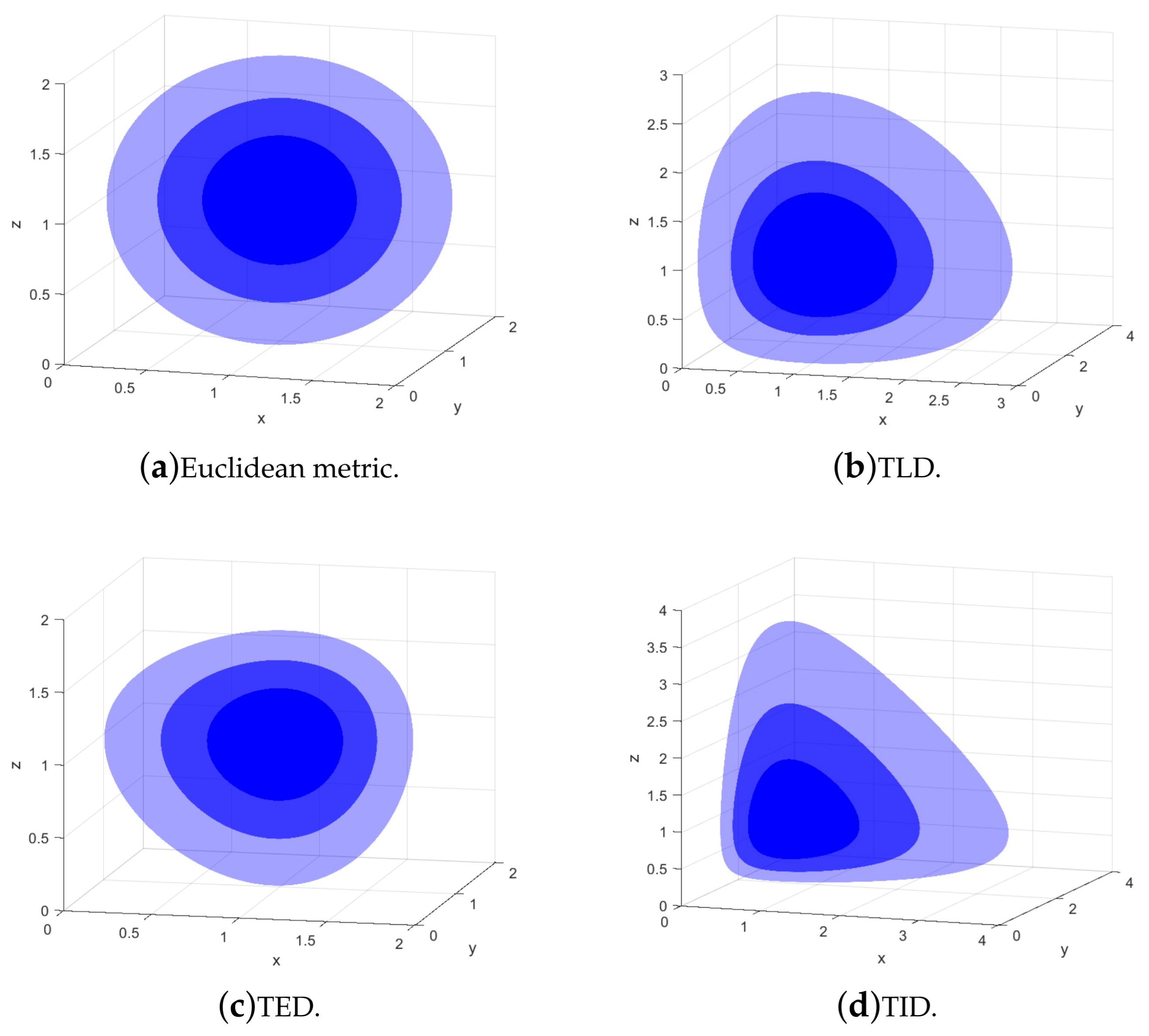
Figure 2.
Denoised-raw point cloud contrast.
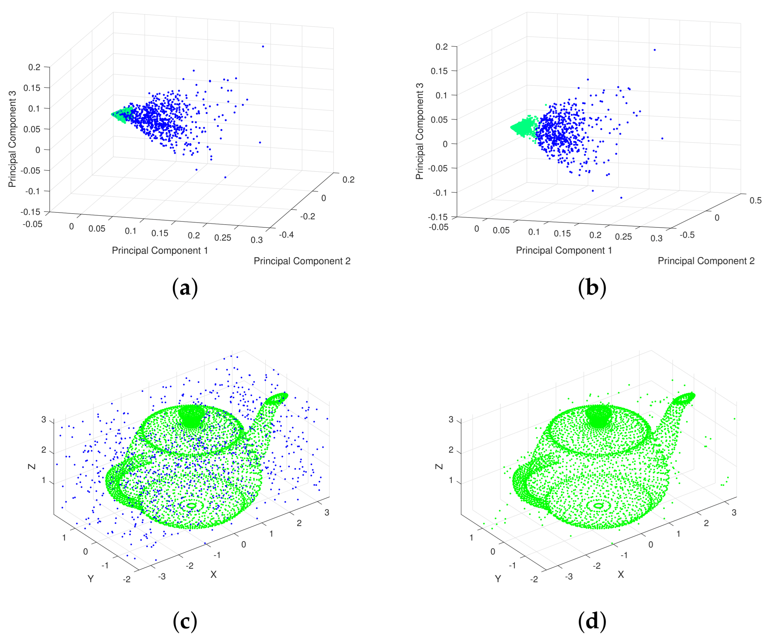
Figure 3.
Comparison of loss functions.
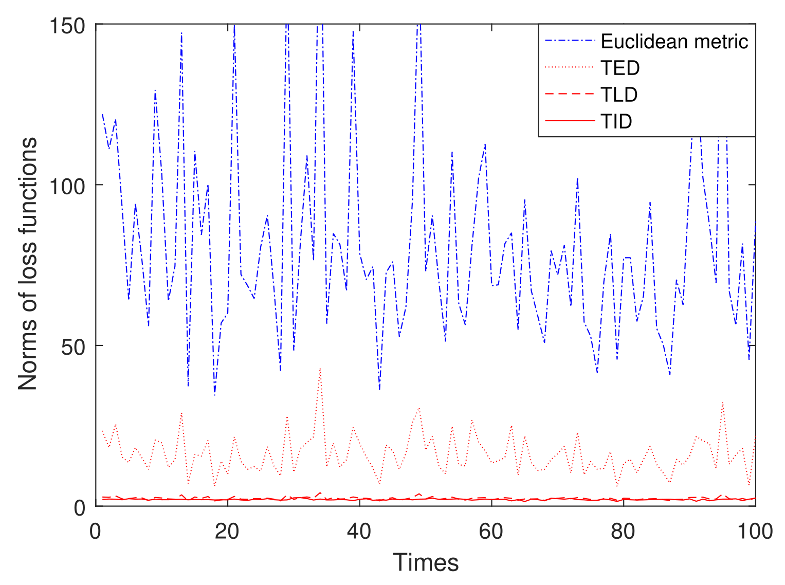
Figure 4.
Comparison of the loss functions between LEM and TLD mean.
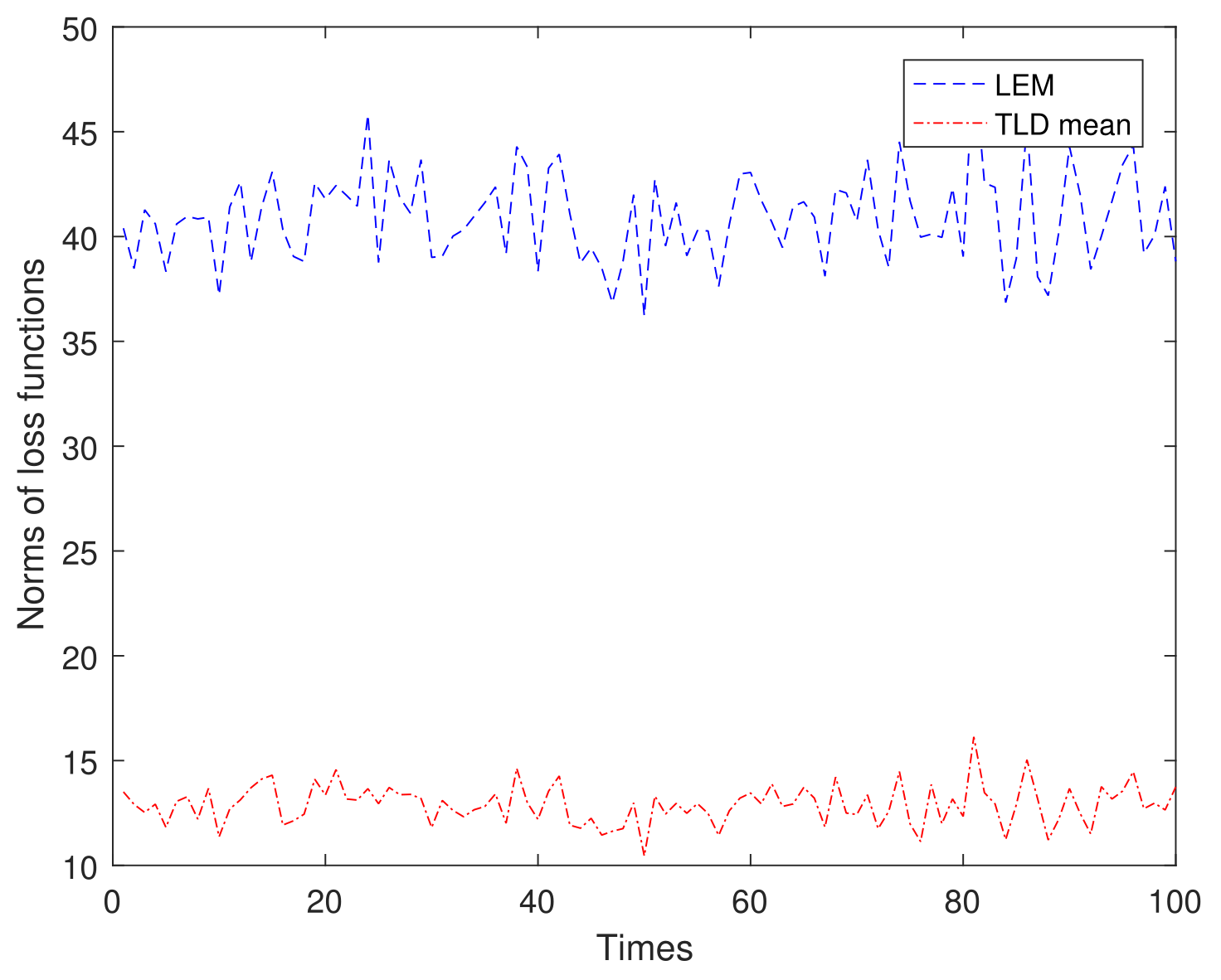

Table 1.
Comparison of denoising results.
| Metric | SNR=10 | SNR=2 | SNR=1 | ||||||
|---|---|---|---|---|---|---|---|---|---|
| TPR | FPR | SNRG | TPR | FPR | SNRG | TPR | FPR | SNRG | |
| Euclid | 100% | 80.24% | 24.62% | 96.17% | 69.14% | 39.09% | 92.38% | 62.32% | 48.24% |
| TLD | 100% | 51.81% | 93.02% | 99.54% | 38.19% | 160.67% | 93.76% | 38.86% | 141.25% |
| TED | 100% | 57.59% | 73.64% | 100% | 44.65% | 123.97% | 97.40% | 47.52% | 104.97% |
| TID | 100% | 46.99% | 112.82% | 90.24% | 26.81% | 236.60% | 87.01% | 27.41% | 217.41% |
Disclaimer/Publisher’s Note: The statements, opinions and data contained in all publications are solely those of the individual author(s) and contributor(s) and not of MDPI and/or the editor(s). MDPI and/or the editor(s) disclaim responsibility for any injury to people or property resulting from any ideas, methods, instructions or products referred to in the content. |
© 2025 by the authors. Licensee MDPI, Basel, Switzerland. This article is an open access article distributed under the terms and conditions of the Creative Commons Attribution (CC BY) license (http://creativecommons.org/licenses/by/4.0/).
Copyright: This open access article is published under a Creative Commons CC BY 4.0 license, which permit the free download, distribution, and reuse, provided that the author and preprint are cited in any reuse.


