
Submitted:
10 October 2023
Posted:
11 October 2023
You are already at the latest version
Abstract
Conceptual distance refers to the degree of proximity between two concepts within a conceptualization. It is closely linked with semantic similarity and relationship, but its computation relies entirely on the context of the given concepts. The DIS-C algorithm, which requires using search algorithms such as Breadth First Search, represents an advance in computing the semantic similarity/relation regardless of the type of knowledge structure and semantic relationships. The shortest path algorithm facilitates the determination of the semantic closeness between two indirectly connected concepts in an ontology by propagating local distances. This process is implemented for each concept pair to establish the most effective and efficient paths to connect these concepts. The algorithm identifies the shortest path between the concepts, allowing for the inference of the most relevant relationships between them. This approach contributes to developing a comprehensive understanding of the ontology and enhances the accuracy and precision of the semantic representation of the concepts. However, one of the critical issues is associated with the computational complexity due to the nature of the algorithm, which is errorn3. This paper studies alternatives to accelerate the DIS-C based on approximation and optimized algorithms, focusing on Dijkstra, pruned Dijkstra, and Sketched-based algorithms to compute conceptual distance. Based on the experiments, we discovered that the bottleneck can be avoided using the proposed 2-hop coverages, bringing DIS-C almost linearity.
Keywords:
conceptual distance
; shortest path algorithms
; accelerated calculation
; computational complexity
MSC: 68Q25
1. Introduction
The spread of information and communication technologies has significantly increased the available information. Thus, we can interpret this information through concepts. Conceptual matching is essential for human and machine reasoning, enabling problem-solving and data-driven inference. Researchers studying the human brain use the term "concept" to describe a unit of meaning stored in memory. The ability to relate concepts and generate knowledge is inherent to humans. Giving computers this capability is a significant advance in computer science.
Transferring the relationship between concepts from the human domain to the computational domain is complex. Sociocultural and language aspects are closely related to the types of concepts an individual acquires. Determining the similarity between concepts so that a computer can process them is one of the most basic and relevant problems in various research fields.
Over time, people have explored various structures and methods to represent the semantic relationships underlying conceptual distance. The graph is one of the most used abstract data types to represent this information, designed to model connections between people, objects, or entities. Nodes and edges are the two main elements of a graph. In addition, graphs have specific properties that make them unique and valuable in different applications.
In recent years, conceptual graphs generated from ontologies have gained relevance. These graphs are strongly connected, where each concept is a vertex, and two edges represent each relationship (one in each direction). Consequently, applying different graph theory search algorithms to study and analyze the relations represented in the conceptual graph is possible. The shortest-path algorithms are crucial in solving different optimization problems. The primary purpose of these algorithms is to find the path with the minimum cost or distance between a given pair of vertices in a graph or network. The study of the shortest path algorithms and proposing different approaches to reduce computational cost have been deeply studied, considering the research works proposed by Dreyfus (1969) [1], Gallo and Pallottino (1988) [2], Magzhan and Jani (2013) [3], Madkour et al. (2017) [4].
Some research works offer different techniques and optimizations for efficiently applying the shortest path algorithm to handle massive data. Fuhao and Jiping (2009) [5] proposed a novel adjacent node algorithm that is more suitable for analyzing networks with massive spatial data. Chakaravarthy et al. (2016) [6] introduced a scalable parallel algorithm that significantly reduced inter-node communication traffic and achieved high processing rates on large-scale graphs. Yang et al. (2019) [7] focused on routing optimization algorithms based on node-compression in big data environments, addressing the common problem of finding the shortest path within a limited time and limited nodes passing through. Liu et al. (2019) [8] presented a navigation algorithm based on a navigator data structure, which effectively navigates the shortest path with high probability in massive complex networks.
Unfortunately, the shortest path algorithm can propagate local distances to determine the distance between two not directly connected concepts by a relation in the ontology. This process is applied to each pair of concepts, making establishing semantic closeness possible. However, calculating these distances has a high computational cost since traditional algorithms have a complexity of around , which is disadvantageous with massive graphs. In this paper, we use the DIS-C algorithm Quintero et al. (2019) [9] as a basis for computing the conceptual distance, which has a complexity to try to make it more efficient.
According to Mejia Sanchez-Bermejo (2013) [10], measuring the conceptual distance between words has been the object of study for many years within the areas of linguistic computing and artificial intelligence because it represents a generic procedure in a wide variety of applications, such as natural language processing, word disambiguation, detection and error correction in text documents, text classification, among others. Reducing the computational cost of calculating conceptual distances for each pair of concepts in massive graphs will accelerate semantic similarity computation. Consequently, it will have practical benefits and contribute to developing more efficient applications to solve practical problems, for instance, reducing the computational time required to search pairs of documents with high semantic similarity in large data sets composed of millions of documents. Additionally, it expands the understanding of the phenomenon of semantic similarity in computing systems based on conceptual graphs. Research and developing efficient algorithms that reduce computing time by combining approximation or analytical techniques is vital to advance the study of semantic similarity.
The manuscript is organized as follows: Section 2 comprises the state-of-the-art that refers to this field. Section 3 presents an analysis of the complexity of the DIS-C algorithm to reference the parts to be improved accurately, the algorithms proposed to improve performance, and the demonstration of its accuracy and the associated computational complexity. In Section 4, we establish the execution scenarios, which include the total number and type of tests. Section 5 presents the experimental results and their discussion. Finally, Section 6 outlines the conclusion and future work.
2. Related work
2.1. Semantic Similarity
Conceptual distance is closely related to semantic relationship and semantic similarity. The semantic relationship, on the other hand, is not necessarily conditioned by a taxonomic relationship; in general terms, these relationships are given by any relationship between concepts, such as meronymy, antonymy, functionality, cause-effect, holonymy, hyponymy, hyperonymy, and so on. On the other hand, we define conceptual distance as the space that separates two concepts within a conceptualization; in other words, it is the degree of proximity between the concepts Quintero et al. (2023) [11]. We can define a rule that indicates conceptual closeness about how close to 0 (in terms of distance) the assigned value is. However, computing such distance depends entirely on the context of the concepts. However, to calculate it, the concepts must first be represented in a model that allows expressing the semantic relationships and defining the measurement metric from the different underlying structures and representations.
In the network model, ontologies are used to face the problem of formally representing the semantics of the information and its relationships Meersman (1999) [12]. The above structures assess the conceptual distance between terms. The present work considers the assumption that we can represent an ontology as a strongly connected graph (conceptual graph); in this context, some authors have proposed many approaches to evaluate the closeness between concepts.
In the literature, authors employ four groups of methods, models, and techniques to compute semantic similarity: a) edge counting-based, b) feature-based, c) information content-based, and d) hybrids. In this work, we use information content-based methods due to their direct relationship with calculating conceptual distance as a measure to determine semantic similarity. The underlying knowledge base offers these methods a structured representation of terms or concepts connected by semantic relationships, also offering a semantic measure free of ambiguity since we consider the terms’ real meaning Sanchez et al. (2012) [13].
2.1.1. Edge counting-based methods
Edge-counting methods consider an ontology a connected graph, where the nodes are concepts, and the edges are relations (almost always taxonomic). The number of edges separating two concepts establishes the similarity between them. Rada et al. (1989) [14] presented one of the first outcomes, proposing a metric called “Distance” defined as minimum number of edges that separate a and b. Despite the effectiveness of its algorithm, one of its most significant drawbacks is its inefficiency when using relationships other than “is-a”.
Wu and Palmer (1994) [15] proposed a measure based on a semantic representation, where they define each verb by a set of concepts in different conceptual domains. Thus, they organized such representation in a hierarchy, formally demarcating its measurement.
In the study presented by Hirst and Stonge (1995) [16], the edge-counting method is extended by considering non-taxonomic semantic links in lexical strings. Such an idea was based on considering all types of relationships found on the WordNet [17], along with the intuition that the longer the path and the more direction the relationship changes, the less the similarity. In such work, authors interpreted the directions in the relationship of the lexical chain as ascending (hypernymy and meronymy), descending (hyponymy and holonymy), and horizontal (antonymy).
Li et al. (2003) [18] proposed a similarity measure as a function that considers the attributes of the shortest path length, depth of ontological information, and local density in a nonlinear function. This research employed a hierarchical structure with relationships of the type “is-a” or “is a type of”.
More recent investigations within the edge count method are mainly based on already established measures, such as those mentioned above with slight variations or the addition of penalty factors to calculate the shortest distance between concepts. An example is the work proposed by fullciteshenoy2012new, inspired by the measure developed by Wu and Palmer (1994) [15].
Thus, Table 1 summarizes the methods based on edge counting we have mentioned; the table contains the expression used to compute the similarity/distance and a brief explanation of the variables involved.
While this method’s class performs well and enjoys simplicity, several limitations hinder their performance. First, they only consider the shortest path between pairs of concepts. It applied to large and detailed ontologies that incorporate multiple taxonomic inheritances; the result is only sometimes the best because the users need to consider several taxonomic paths. Other characteristics that influence the semantics of the concept, such as the number and distribution of common and uncommon taxonomic ancestors, are not considered either. Another problem with edge count measures is that they are based on the notion that all links in the taxonomy represent a uniform distance. In practice, the semantic distance will depend on the granularity and taxonomic detail implemented by the knowledge engineer Sanchez et al. (2012) [13].
2.1.2. Feature-based methods
Feature-based methods are based on the Tversky (1977) [20] similarity model, which in turn derives from set theory, assesses the similarity between concepts based on their properties, subtracting the common and uncommon features of the terms, and attempts to overcome the limitations of edge count-based measures concerning the fact that taxonomic links in an ontology do not necessarily represent uniform distances Sanchez et al. (2012) [13]. These types of measures have the potential to be applied in the calculation of semantic similarity supported by crossed ontological structures, that is, when the pairs of concepts belong to two different ontologies, a milestone that methods based on edge counting are not capable of reaching.
The idea is quite simple: if we imagine three concepts such as “dog”, “bird”, and “sofa”, we can almost instinctively realize that “dog” and “bird” are more similar to each other. This reasoning may be associated with the fact that we identify a “dog” and a “bird” as animals despite not having a direct relationship of kinship. Someone can argue that “dog” and “bird” have more characteristics in common than they would with a “couch”.
One of the first studies to develop a semantic similarity measure based on the hypothesis that the more common characteristics two words have, the more related they are, the research by Lesk (1986) [21] proposed the homonymous measure. The algorithm for calculating this Lesk measure aims to search for the disambiguation of words in texts. The work presented by Banerjee and Pedersen (2003) [22] is an extension of the Lesk measure. It took as reference the terms or synsets provided by WordNet. The idea of performing multiple comparisons sets it apart from the original algorithm. His measure seeks overlaps between the glosses of the synsets themselves, hyperonyms, hyponyms, meronyms, holonyms, and troponyms.
In the modern world, there are multiple sources of information, such as social networks and internet blogs, among others, that provide a large amount of information daily, including terms or concepts (new words, brands, acronyms, among others) uncaptured in domain ontologies or formal taxonomic structures. For this reason, there are works where other sources of knowledge are used, such as Wikipedia. In this aspect, the study of Jiang et al. (2015) [23] evaluates specific existing methods, based on characteristics, under a formal representation of concepts extracted from said source. In general, there is an excellent human correlation, and there are some practical ways to determine the similarity between Wikipedia concepts.
The main drawback of the feature-based approach is its reliance on ontologies or knowledge sources with semantic features such as glosses, and most ontologies rarely incorporate semantic features other than relations [13]. It significantly restricts its use for computing the similarity between concepts; however, this approach has been adopted to calculate the similarity between other data types, such as images or videos.
2.1.3. Information content-based methods
Information content-based approaches arose from the need to improve some of the limitations of edge-counting-based methods. Specifically, Resnik (1995) [24] proposed to complement the taxonomic structure of an ontology with the information distribution of concepts evaluated in the input corpus. Similarly, the author framed the notion of information content (IC) by associating probabilities of the appearance of each concept in the taxonomy. The IC was computed from its occurrences in a given corpus. Therefore, a high IC value indicates that the word is more specific and clearly describes a concept with less ambiguity.
In contrast, lower IC values indicate that the words have a more abstract meaning [25]. The Resnik measure calculates the IC of a concept a according to the negative logarithm of its probability of occurrence , . This measure is closely related to the notion of LCS (Least Common Subsumer) because, according to Resnik’s research, semantic similarity depends on the information shared between 2 terms and a way that represents such measure in a taxonomy. This way, if two terms do not share an LCS, they are considered significantly different.
It is evident that if any pair of terms share the same LCS, the result of semantic similarity is the same; this is one of the main drawbacks of the measure. For this basis, over time, research focused on the notion of the IC, combining the main reasoning of the IC with other ideas that complement its calculation and, in its entirety, semantic similarity.
An example of the above is the work of Jiang and Conrath (1997) [26] based on the notion of IC proposed by Resnik (1995) [24]. The measure proposed by Jiang and Conrath (1997) [26] is a combined model derived from the method based on edge counting by adding the information content as a decision factor. The results showed that a combined approach outperforms the IC approach alone. Thanks to the practical results, such outcomes gave credibility to using the IC as a factor for calculating the semantic similarity and as reinforcement in the computation of the conceptual distance based on finding the shortest path between two terms.
Gao et al. (2015) [27] considered the basis of edge counting methods, that is, the shortest path length between two concepts, and combines it with the IC of the LCS. This way of interpreting relations is close to the work of Jiang and Conrath (1997) [26], and in general terms, this approach is mainly accepted in many research investigations; however, the fundamental difference is in the model used to describe the semantic similarity. Jiang et al. (2017) [28] proposed computing the IC of a concept from Wikipedia. They suggested diverse methods for IC calculation that aim to test which IC calculation method and which underlying similarity measurement approach are suitable for concept similarity calculation in the Wikipedia category structure. The first technique presented the computing of IC using the category structure and the extension of methods founded on Jiang and Conrath (1997) [26] corpus. Table 2 summarizes the IC-based methods. Moreover, we present the expressions used to calculate IC and briefly explain the variables involved.
2.1.4. Hybrid methods
While some of the above mentioned investigations use a hybrid approach, where authors combine two or more techniques for calculating semantic similarity, This section explains the work on which this is based. In [9], we proposed the DIS-C method to calculate the conceptual distance between two concepts in an ontology based on a fundamental approach that uses the topology of ontology to compute the weight of relationships between concepts. Unlike other methods, DIS-C can incorporate various relationships between concepts, such as meronymy, hyponymy, antonymy, functionality, and causation, without needing to represent the source of knowledge in taxonomic or hierarchical structures.
The theoretical foundation of the DIS-C method considers the conceptual distance as the space that separates two concepts within a conceptualization represented as a directed graph. We assumed that the distance is related to the difference in information content provided by the concepts in their definitions. The method assigns a distance value to each relationship type and transforms this into a weighted directed graph, allowing the conceptual structure not to matter. This characteristic means that DIS-C can be applied to any conceptual structure. The only requirement for the algorithm is that the conceptualization be a 3-tuple of elements , where C is a set of concepts, ℜ is the set of types of relations, and R is the set of relations in the conceptualization. With this information, the method can calculate the conceptual distance between each pair of concepts, the weight each type of relationship contributes, and a marginal measure called generality closely related to the IC. The DIS-C algorithm includes a method for the automatic weighting of the graph. In the literature, the weighting in methods based on graphs is too specific to the type of conceptualization, so proposing a general method allows independence concerning the domain.
Thus, we consider DIS-C a hybrid approach because, as we have seen, the computing of the IC (characterized by generality) is used and combined with the calculation of the shortest path between all pairs of nodes to find all the most critical concepts, close to each of the concepts themselves. Section 3.1 presents the analysis of the DIS-C algorithm in more detail. In summary, the method is described through the following steps:
- Assign to each relation an arbitrary conceptual weight defined in each direction of the relationship.
- A directed and weighted graph (conceptual graph) is created where the vertices are the concepts contained in the conceptualization and the edges are the relationships that connect each pair of concepts. Each edge has its counterpart in the opposite direction with different weighting. Finally, to compute the weighting, the generality of each concept is necessary.
- Calculate the length of the shortest paths between each pair of vertices, i.e., diffuse the conceptual distance to all concepts.
2.2. All pair shortest path problem
In the conceptual graph, each node is a concept, and each relation is an edge connecting a pair of nodes. Graph theory techniques can extract the underlying knowledge encoded in the ontology. The natural step is to compute the shortest path to find the distance between concepts that are not directly related. In this step, we find one of the leading technical drawbacks of the approach, and it is the specific issue to be dealt with in this work. When dealing with large graphs, calculating the shortest path between each pair of concepts is computationally expensive. This type of problem in graph theory is known as “All Pair Shortest Path” (APSP) [31].
In [9], we used two well-known algorithms to solve this problem: the Floyd-Warshall and Johnson-Dijkstra algorithms. Floyd-Warshall is based on transitive Boolean matrix closure [32] with computational complexity of 1. At the same time, Johnson-Dijkstra has complexity (when using Fibonacci heaps as a priority queue); however, it requires that there is no negative cycle in the graph and when the complexity is equal to [33].
The APSP is widely related to the matrix multiplication problem (MM); for this explanation, people often use accelerated matrix multiplication algorithms where, in general, there is a cost of [34]. Techniques like divide and conquer [35] or metaheuristic algorithms [36] are also used to optimize the computational cost. Another approach uses new-generation hardware, such as the GPU, to parallelize existing algorithms and thus reduce runtime [37].
Thus, the complexity of the APSP problem has remained open even though it is executed in polynomial time. According to Reddy (2016) [38], most of the algorithms are based on the following two types of computational models:
- Addition comparison model: The shortest path algorithms in this model assume that the inputs are real weighted graphs, where the only operations allowed on reals are comparisons and additions.
- Random Access Machine (RAM) model: In this model, shortest path algorithms assume that the inputs are weighted graphs of integers manipulated by addition, subtraction, comparison, shift, and various logical operations [39].
Most algorithms that solve the APSP problem work on the RAM model. Unfortunately, some of the algorithms are far from practical. We must consider the characteristics of the graph (directed, weighted, complete, among others) to face this problem; the effectiveness of most algorithms depends directly on their properties.
2.2.1. Analytic solutions
The algorithm presented by Johnson (1977) [40] was one of the first to use Dikjstra’s algorithm as a subprocess, in addition to the Bellman-Ford algorithm to remove negative edge weights, thus achieving a total computational complexity of . This complexity improves on the Floyd-Warshall algorithm described by Bernard Roy in 1959, which has a complexity.
Chan (2010) [41] presented an algorithm for the APSP problem with real-weighted general dense graphs. It has a computational complexity of . The base of such an algorithm is on calculating the distance product of two square matrices, and the efficiency is obtained through computational geometry and using rectangular matrix multiplications instead of square matrix multiplications.
Moreover, Peres et al. (2013) [42] studied a specific case of graphs achieving a theoretical time limit of . However, the limitation of the proof is the dependency on the class of complete and directed graphs with an edge weight independently and uniformly at random between . The algorithm proposed by Peres et al. (2013) [42] is considered a variant of Demetrescu and Italiano (2004) [43]. The notion of local shortest paths (LSP) is the base of such algorithms.2 Roughly speaking, the algorithm presented by Demetrescu and Italiano (2004) [43] is a parallel implementation of Dijkstra’s algorithm from each node of the graph, with the difference that it only examines the LSP, following a series of specific rules using a priority queue. This algorithm correctly finds all the shortest paths in the graph in time .
Williams (2018) [44] proposed the fastest known algorithm for the APSP problem with dense graphs. The computational complexity is . The algorithm uses Monte Carlo and algebraic techniques to reduce the computation time in multiplying rectangular matrices. It is a non-deterministic algorithm. However, the investigation also showed that the APSP could be solved deterministically in a time for a using a suitable deterministic polynomial transformation. Later, Chan and Williams (2016) [45] showed that the problem can be solved deterministically in time .
Brodnik and Grgurovic (2017) [46] developed an algorithm that sub-processes any other single source the shortest path (SSSP) algorithm, which solves APSP with an asymptotic limit ; where is the number of different edges in the shortest paths, and is the time the algorithm, solves the SSSP problem. This approach is very similar to the hidden path algorithm [47], which is essentially a modification of Dijkstra’s algorithm to make it more efficient in solving APSP. The primary difference between the two methods is that the hidden path method only works with Dijkstra’s algorithm, while the Brodnik and Grgurovic (2017) [46] algorithm works for any arbitrary algorithm that solves SSSP. The authors used the Johnson weighting technique, topological ordering, and the propagation algorithm to solve the APSP in time for directed acyclic graphs with arbitrary weighting.
Kratsch and Nelles (2020) [48] considered the APSP within the framework of efficient parameterized algorithms (FPT in P). Specifically, the authors investigated the influence of two parameters: clique-width () and modular-width (). The result is an efficient and combinatorial algorithm for graphs with non-negative weighting in the vertices, such that the algorithm is executed in time using the parameter and for . In addition, when fast matrix multiplication can be used, the time is reduced to using the algorithm defined by Yuster (2009) [49] as a black box for the matrix multiplication. One of the differences with other algorithms is the particularity of working with graphs weighted in the vertices and not in the edges.
In summary, despite the great interest in the APSP problem, there are only minor advances in computational complexity over for general graphs based on the computation of the distance product, closely related to matrix multiplication. Although subcubic algorithms exist, they only take advantage of properties of specific graphs or benefit from sparse graphs, so up to now, there is no genuinely subcubic combinatorial algorithm. Table 3 describes the algorithms developed with their computational complexity over time, and Figure 1 shows the execution time comparison of each algorithm.
2.2.2. Approximation solutions
Although we can solve the APSP problem in polynomial time, its application for large graphs is not feasible in practice. For this basis, it is interesting to analyze heuristic and metaheuristic methods and approximation algorithms in this class of problems. The clear advantage of this approach is the speed gain, while its disadvantage is the accuracy of the computation. In the literature, authors use a few relevant investigations of this class of algorithms in the APSP problem: genetic, evolutionary, and optimization algorithms per ant colony.
Attiratanasunthron and Fakcharoenphol (2008) [59] presented a rigorous analysis of the running time for ACO in a shortest-path problem. Its n-ANT algorithm is inspired by the 1-ANT [60] and the AntNet [61] algorithm. In Horoba and Sudholt (2009) [62], the n-ANT algorithm to solve APSP is formalized and optimized. We will call this algorithm that is a generalization of presented in the same research study. This algorithm solves the single source shortest path problem. The computational complexity of is , where is the maximum degree of the graph, l the maximum number of edges in any shortest path, and .
On the other hand, Chou et al. (1998) [63] used a hierarchical approach to decompose a network (graph) into several smaller subnets. In this way, when it is necessary to search for a shorter path, it is evaluated in a smaller graph. However, the shortest path may be different. The shortest paths of all pairs of nodes can be approximated through various constraint mechanisms by exploring a search space smaller than that of the original graph. The authors compare the computational complexity between Dijkstra’s algorithm and two versions of the algorithm called HA: Best HA, which obtained the best results regarding the error of the shortest paths, and the Nearest HA, the fastest execution instance. Dijkstra had no error percentage, while the Nearest HA had 21.5% and Best HA had 4.68%. Concerning runtime, Nearest HA was 15 times faster than Dijkstra and Best HA only twice. Mohring et al. (2007) [64] presented a similar work; however, their study only focuses on the shortest path to a single source. So, the hypothesis that it can be generalized for APSP is supported.
Other works that do not focus on graph partitioning but do speed up the asymptotic limit concerning are Baswana et al. (2009) [65] and Yuster (2012) [66]. The first one points to unweighted and undirected graphs, where the merit lies in presenting the first algorithm to calculate APSP with a 3-approximation, this means that for each pair of vertices , the distance reported by the algorithm is not greater than , such that is the actual shortest distance of the path. The article also presents two more algorithms for a 2-approximation, specifically, the first corresponds with complexity and , the second, and . The clear advantage is that there is a defined limit of error.
Finally, there is the Sketch-based approach. Multiple investigations have been considered, but two extensive processes can be identified globally. The first is pre-processing, where the result is a data structure that allows consulting the distance between two nodes. This data structure, a distance oracle, was introduced in [67]. The second process is related to queries, where it is a question of making queries to the oracle and for it to return, in a specific time limit, the result of the shortest distance between two nodes.
Unlike exact algorithms, these algorithms reduce time by several orders of magnitude. Das Sarma et al. (2010) [68] is one of the first studies to adopt this approach for complex graphs with hundreds of millions of nodes and billions of edges. The description of the algorithm is simple: sample a small number of node sets from the graph, called seed node sets. Then, for each node of the graph, the nearest seed is searched in each of these sets of seeds. The sketch of a node is the set of closest seeds and the distance to them. Thus, given a pair of nodes u and v, the distance between them can be estimated by looking for a common seed in their sketches. Although there are no theoretical guarantees of the degree of optimization of the method for directed graphs, the results showed a better average, close to the actual distance, when applied to directed graphs than to undirected graphs.
Wang et al. (2021) [69] centered on finding all shortest paths in huge-scale undirected graphs. Despite having practically the same approach, what makes it different from the work of Das Sarma et al. (2010) [68] is that Wang et al. (2021) [69] considered the computational complexity to perform the preliminary calculation. This task’s standard method applies a BFS algorithm to the seed node sets. It is well known that the complexity of BFS is when using an adjacency list or for an adjacency matrix. This complexity is a drawback when processing extensive graphs. For this reason, they considered whether it is possible to speed up the preliminary computation with the [70] pruned reference point labeling technique, that is, applying a pruned BFS. The specific results for this stage showed a linear time for its construction, that is, . The results showed a notable improvement, especially in runtime, for large graphs.
3. Methods and materials
The solution presented combines several approaches to solve the APSP, although the DIS-C algorithm consists of other processes whose computational cost is non-significant.
3.1. Analysis of the DIS-C algorithm
Quintero et al. (2019) [9] detailed two algorithms; the basic one, which calculates the conceptual distance given a conceptualization and the weights for each relationship type . Such an algorithm consists of converting the conceptualization K into a graph with and through which we compute the conceptual distance by calculating the APSP in the graph G. The second algorithm enables automatic weighting, which allows the conceptual distance to be computed automatically without providing the weights of the relationship types. It is precisely this algorithm that we want to speed up. Figure 2 shows the flowchart corresponding to the DIS-C algorithm with automatic weighting3, which will subsequently be referred to simply as DIS-C.
As mentioned, the APSP algorithm has the most significant influence on computational complexity. Up to this point, we can set that the computational complexity of the DIS-C algorithm is for a conceptualization with n concepts4.
3.2. The pruned Dijkstra
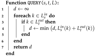
The pruned Dijkstra algorithm is an optimized version of Dijkstra’s algorithm in which unnecessary paths are removed in the search, keeping a list of pending nodes and choosing to expand the one with the minimum distance in the list. If we find a path longer than the currently known shortest path to any node during expansion, then that path is discarded and not considered again. In this way, the pruned Dijkstra algorithm reduces the number of paths to be considered. It is a generalization of the PLL (Pruned Landmark Labeling) method for undirected weighted graphs [70]. The PLL method is based on the idea of 2-hop coverage [72], which is an exact method. It is defined as follows: let be an undirected and weighted graph; for each node , the cover is a set of pairs , where u is a node and is the distance from u to v in the graph G. All covers are denoted as indexed . To calculate the distance between two vertices, s and t, we use the search function (Q), as shown in Eqn. 1. L is a two-hop cover of G if for any .
In the case of weighted directed graphs, it is necessary to calculate two indexes; the first contains the coverage of all the nodes, considering the incoming edges. The second considers the outgoing edges. The way to consult the distances has a minor modification, but the idea remains the same. Such change can be observed in Eqn. 2.
A naive way to build these indexes is through two executions of Dijkstra’s algorithm. Although this method needs to be more obvious and effective, we will explain the details to discuss the next method. Let , start with an empty index , where . Suppose Dijkstra is used on each vertex in the order . After the k-th Dijskstra on a vertex , the distances of are added to the coverages of the vertices reached, whereby for each with , where is the distance from node u to node v within the graph G. It is important to mention that the coverages of the vertices reached are not changed, which implies for each with . By performing this procedure starting with , the same result can be obtained but considering the output edges.
Thus, and are the final indices contained in . Obviously, for any pair of vertices, therefore and are the 2-hop covers of G. This is because, if s and t are reachable, then and .
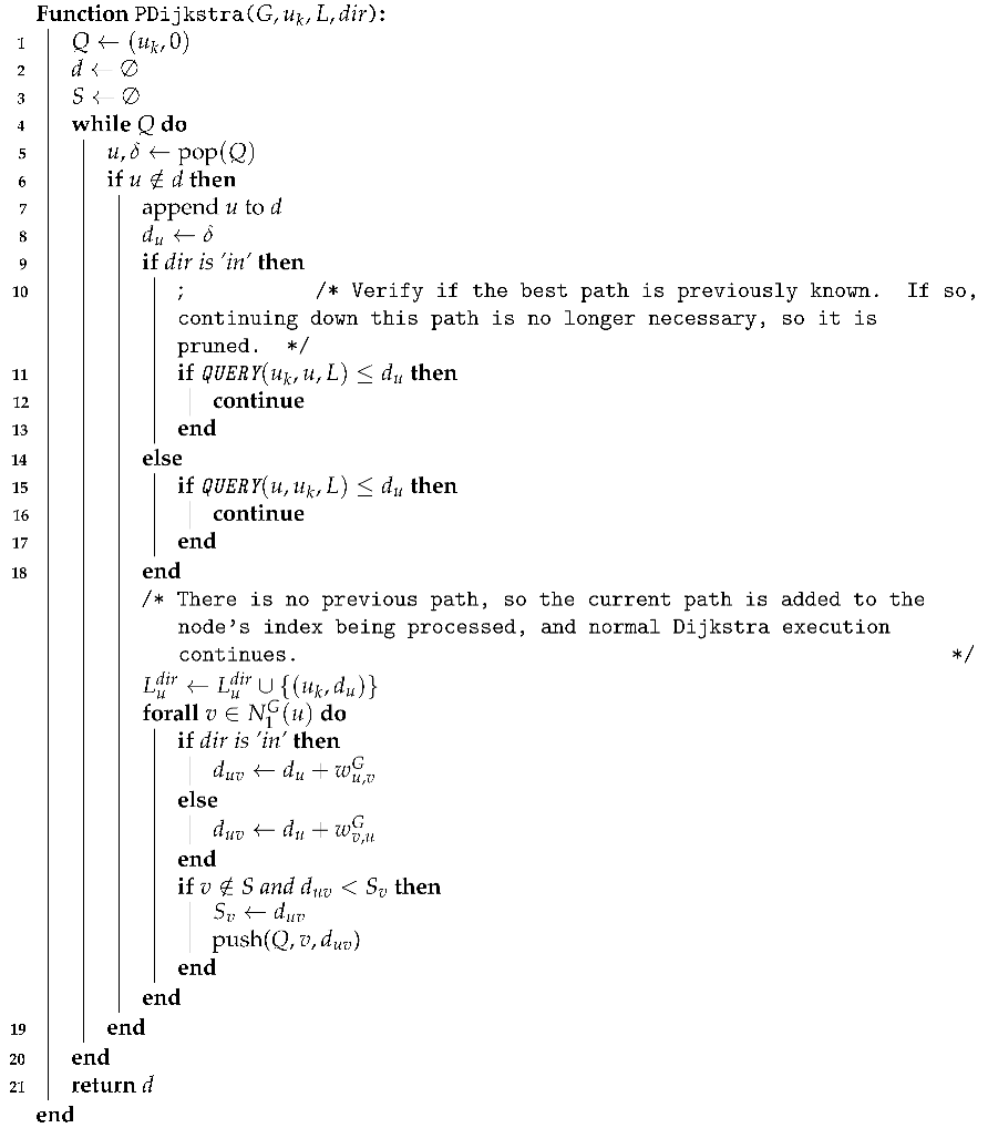
As mentioned at the beginning of the description, this way of creating indexes could be more efficient. For this reason, pruning is added to the naive method. This technique reduces the search space considerably. Like the naive method, a pruned search is conducted with Dijkstra’s algorithm starting from the vertices in the following order: . Start with a pair of indices , and create indices , from and , respectively, using the information obtained by the k-th execution of pruned Dijkstra for vertex .
The pruning process is as follows: suppose we have the indices and and we execute the pruned Dijkstra from to create a new index . Assuming that we are visiting a vertex u with distance . If , then we prune u, that is, we do not add to and we do not add any neighbors of u to the priority queue. If the condition is not met, then is added to the cover of u, and Dijkstra is executed as normal. As with the naive method, we set and for all vertices that were not reached in the k-th execution of the pruned Dijkstra. In the end, and are the final indices contained in .
Figure 3 shows an example of the algorithm acting on the graph represented in the figure, taking the order of execution as . The first pruned Dijkstra from vertex one visits all other vertices, forward and reverse (see Figure 4a and Figure 4b). During the next iteration from vertex 8 (Figure 5e), when node one is visited, given that 1, vertex one is pruned and none of its neighbors are visited anymore; the same occurs in the opposite direction (see Figure 5f). With these two executions, it is possible to cover all the shortest paths, and once the process is executed on the remaining vertices, they will only refer to themselves. The pruned Dijkstra algorithm is described in Algorithm 2, and the whole algorithm for constructing indices is presented in Algorithm 1.
| Algorithm 1:APSP_PDijkstra |
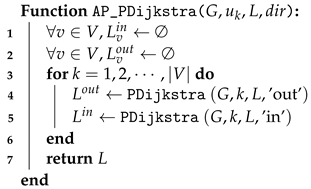 |
We executed the pruned Dijkstra in order ; and arbitrarily chose the order of the vertices; however, it is relevant for a good algorithm performance. Ideally, start from central vertices so that many shortest paths pass through them. There are many strategies to order the vertices; some of the most used ones apply to order by centralities. In this work, we choose the order of the vertices by the degree of centrality. The graphs generated by semantic networks behave like networks without scale, where high-degree vertices provide high connectivity to the network. In this way, the shortest path between two vertices will likely pass through those nodes.
| Algorithm 2:The Pruned Dijkstra |
 |
|
Algorithm 3: Check distance from source to target nodes according a 2-hop cover
|
 |
3.2.1. The pruned Dijkstra analysis
To prove the correctness of the method, it suffices to show that the algorithm computes a two-hop coverage, that is, for any . Let be the index built without the pruning process, so it is a two-hop coverage; is the index built by applying the pruning process. Since there exists a node such that , and , the goal is to show that also exists in and .
Theorem 1.
For , and ,
Proof.
Let , assume there is a path between them, j the smallest number such that , and . We must show that and also lie in and respectively; that is to say that . To prove that , first, for any , suppose , where is a path between a and b. If we assume that , by inequality:
Since and , it contradicts the fact that j is the smallest number. Therefore, for no .
Now, we prove that . Suppose we execute the j-th Dijkstra pruned from node to construct index . Let . Since there is no for , it means that there is no vertex in the i-th pruned Dijkstra iteration that covers the shortest path of to t, therefore . Consequently, vertex t is visited without pruning and is added.
Finally, suppose we execute the j-th Dijkstra pruned from , but this time to build . If s and t are reachable in G, it means that there is a path between and s taking into account the input edges, or what is the same, there is . Since we already proved that for , it means that is a neighbor of s or , and since is the initial vertex of the path , then is the least distance neighbor sharing s. In any of the cases , therefore the node s is visited without pruning (remember that it is considering the input edges). Consequently is added. □
As mentioned, the order in which the nodes are processed influences the algorithm’s performance. Is there an order of execution such that the construction time is the minimum possible? The answer is yes; however, finding such an order is challenging. So, there are two approaches: the first is to find the minor nodes that cover all the shortest paths, which is a much bigger problem since this is an instance of the minimum vertex coverage problem that is NP-hard. The second approach is a parameterized perspective; specifically, the explored parameter is the width of the tree. It also relies on the process of centroid decomposition of the tree [73]. This approach deduces the following lemma; the formal proof is made in [70].
Lemma 1.
Let w be the width of the graph of G. There is a vertex order with which the pruned Dijkstra method executes in time for preprocessing, stores an index with space and answers each query in time.
Considering that this research study does not look for minimum two-hop coverage, using the upper bound of for the algorithm can be considered an inconsistency. Since there is no guarantee that the chosen order (degree centrality) is the same as the order necessary to achieve such computational complexity, however, what we concluded for our implementation is that it cannot be faster than the one theoretically obtained using the order with which . That is, our implementation has a lower bound . Also, in terms of Dijkstra’s algorithm, we can hypothesize that the construction of the coverage using the pruned process, regardless of the order of execution, is much smaller than for the construction of the naive coverage in highly connected graphs, that is to say, that .
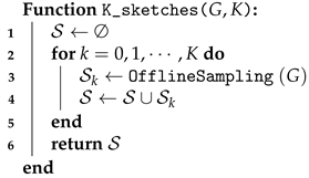
3.3. The sketches
Sketch-based algorithms are methods comprising two general processes: offline and online. In the offline process, the sketches (that are crucial nodes, initially random) are computed from which the shortest path to all the other nodes is calculated. In the online process, we compute the closest distance between a pair of nodes from the closest common sketch between them.
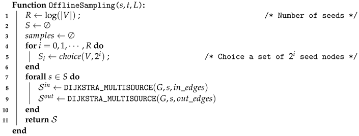
The offline process consists of sampling sets of seed nodes, each containing a subset of size . From each set, the closest seed of each node is stored together with its distance; that is, for each node u, a sketch of the form SKETCH is created. Therefore, the final size of the sketch for each node is . This construction can be made with Dijkstra’s algorithm. The node closest to u is called the seed of u. This procedure is executed k times with different sample sizes. At the end of the k iterations, we obtain seeds for each node.
As with the previous algorithm, we must compute two sketches for each node. The first SKETCH and SKETCH representing the distance from node to the nearest seed and vice versa. We do this by running the search algorithm twice; one considering the input edges, the other with the output edges.
We can randomly choose S, using some criteria to bias our choice. For example, we can discard those nodes whose degree is less than two. We can also take advantage of the graph’s structure, and its specific properties5. In the Algorithm 4, the proposed pseudocode is shown to generate the sketches of each node.
| Algorithm 4:Sketches_DIS-C: offline sampling |
 |
For each sample, we obtain the closest seed node and its distance for each node. This process is done with the classical Dijkstra multi-source algorithm. In this way, the seed nodes for each are computed (see Algorithm 5).
| Algorithm 5:Sketches_DIS-C: k sketches offline |
 |
In each iteration, we generated a sketch from an offline sample; therefore, at the end of the algorithm, there will be seeds for each node.
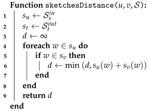
The second process of the method is the online one. The calculation of the approximate minimum distance between nodes u and v is done by looking at the distance from u and v to any node w that appears in both as in . So, we compute the path length from u to v by adding the distance from u to w plus the distance from w to v. The minimum distance is taken if there are two or more common nodes w. Algorithm 6 shows the proposal to perform said calculation.
| Algorithm 6:Sketches_DIS-C: k sketches online |
 |
Finally, to solve the APSP problem, it is necessary to create another algorithm that it executes for each pair of nodes (Algorithm 7).
| Algorithm 7:Sketches_DIS-C: k sketches online APSP |
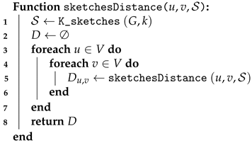 |
Figure 5 shows an example of the described procedure. The graph of Figure 3 is taken as a reference. Since there are 12 nodes, the number of seed sets is 3 (), and the size of the sets are 1, 2, and 4, respectively. The nodes in each set are 1; for the first, ; for the second, and , for the last.
In the first iteration (Figure 5a), all the nodes have node 1 in their coverage; this also happens for the input edges (see Figure 5b). In the second iteration (Figure 5c and Figure 5d), the coverages do not change since node three does not cover any path shorter than those already covered by node 1, finally, in the last iteration (Figure 5e and Figure 5f), we have node 8 in the seed set, this covers the shortest path of its neighbors, except those that are also in the set; therefore, nodes 5, 12 and 9 will have 8 in their coverage. On the other hand, nodes 2 and 7 are contained in their respective coverage.
3.3.1. Sketches analysis
In the sketches-based method, there is no accuracy test for general graphs. It means that the method does not guarantee exact node labeling to answer the exact distance between all pairs of vertices. As far as computational complexity is concerned, it is easy to determine.
Theorem 2.
For a set of nodes such that the size of said set is for , the computational complexity of the algorithm is .
Proof.
We know that the sketch-based method selects a number w founded on the number of nodes in the graph, that is, . Then, given w, subsets of nodes are created for such that the size of each one is . It can be seen that . For each of the subsets, the multi-source Dijkstra algorithm is executed, with the aim of finding, for all the nodes of G, the closest node of the set. Dijkstra’s algorithm from multiple sources has a complexity of ; for each subset of nodes, it is necessary to apply (independent of size) a single execution of Dijkstra’s algorithm. Therefore, since there are w subsets of nodes, w Dijkstra processes from multiple sources must be executed; that is to say, in total, we reach a complexity of . □
In the implementation carried out in this work, we determined w by a logarithmic function , where . In this way, we ensured that . Therefore, for the implementation made, the method has a complexity of .
4. Experiments and execution scenarios
This section specifies the different experiments carried out, the proposed datasets, and the execution environments.
4.1. The datasets
Datasets are pairs of words to which, through human judgment, a numerical value is assigned. We divide these sets into two families: those that measure semantic similarity and those that measure semantic relatedness. These sets are described in Table 4.
Therefore, we run the process through a script that, for each data set, takes a couple of words, generates the conceptual graph that connects them, and applies the DIS-C algorithm to find the conceptual distance. We repeat this process with all the pairs of words, and in the end, all the graphs generated from a set of words are unified to obtain a graph with all the pairs of words in the set. We also apply the DIS-C algorithm to the unified graph from this last execution, where the conceptual distances are registered. The objective of applying DIS-C to graphs that connect only a couple of words is to measure the runtime with different sizes of graphs and thus have a much more extensive record.
4.2. Evaluation metrics
We divide the evaluation metrics for this research work into performance and semantics. The first corresponds to the running time measurement, related to the graph’s number of nodes and edges. Semantic metrics measure the precision in estimating similarity, using the Pearson correlation factor (Equation 3), the Spearman rank correlation factor (Equation 4), and the harmonic score (Equation 5).
Pearson’s correlation compares human similarity vectors and has been widely used to evaluate similarity estimation methods between words and concepts. Spearman’s rank correlation ranks invariants and allows comparison of the intrinsic power of word similarity measures. In addition, we used harmonic scoring, which combines Pearson and Spearman correlations to provide a single weighted score for assessing word similarity methods. These correlation measurements are essential for evaluating and comparing similarity methods in the literature.
5. Experimental results
In this section, we describe the results of the different experiments. In the first part, we analyze the performance metrics on the generated graphs; also, we compare the control algorithm and those proposed. The second section analyzes the results of the semantic metrics.
5.1. Generated graphs and performance
We generated a graph connecting each pair of words for each dataset to generate the corresponding unified graphs later. Table 5 shows the size of these graphs. The last row of the table (labeled ’All’) refers to the union of all graphs; additionally, algorithms were applied to this graph.
Below are a series of graphs related to each proposed algorithm’s runtime. Figure 6 shows the runtime of the control algorithm, the pruned Dijkstra algorithms, and Sketches. At specific points, the runtime is increased in a “abnormal” way; this is due to a parameter other than the size of the graph; specifically, it is the convergence threshold of the algorithm. It indicates that more iterations were necessary for this dataset, particularly the graph structure, to reach the threshold.
The convergence threshold is a function of the total generality of the graph, that is, the sum of all the generalities of each node. The total generality of the graph depends on the distance value between each pair of nodes provided by the APSP algorithm; for this reason, the algorithms that obtain the shortest actual distance always reach the convergence threshold in the same number of iterations. In this case, there is the control algorithm and the pruned Dijkstra. On the other hand, the Sketches algorithm varies in the number of iterations to reach the threshold; however, as a general rule, such many iterations cannot be less than the number reached by the control algorithm. The reason for this is that the control algorithm obtains the exact shortest distances, so the total generality of the graph is the minimum possible. Since it is known that the Sketches algorithm (and any other approximation algorithm) cannot compute the shortest distance less than the real one, then the generality of the graph cannot be less than the minimum generality.
In the same Figure 6, it can be seen that most of the proposed algorithms have a longer runtime than the control algorithm; this is mainly due to the density of the graphs, that is, the generated graphs have few edges and can be considered sparse graphs. It is noted that only the Sketches algorithm with stays below the time of the control algorithm. However, it is not a considerable acceleration. For the acceleration to be significant, it must be reduced by at least one order of magnitude, considering that the runtime is in the order of days in the results analyzed. Since the proposed algorithms are divided into two significant processes (construction and query), we break down the runtime these two processes take separately. Figure 7 illustrates this particular task.
The query time is the bottleneck in the algorithms. In the complexity analysis of the query process, we established that the complexity of the Sketches algorithm depends on the size of the coverages, and these are a function of k, so the behavior when increasing the value of k is predictable, as shown in Figure 7. In the case of the pruned Dikstra algorithm, the size of the coverages is enormous for more general nodes and decreases as a function of such generality. It motivates some nodes to find their shortest distance, which will take longer; this behavior speeds up the total query time. Although a binary search can be used instead of a linear one, it does not underestimate the quadratic factor inherent to APSP and whose behavior is reflected in the results. This inconvenience led us to conjecture that it is possible to calculate the generality of the graph only with the coverages of the nodes. It means that solving APSP to calculate the generality is unnecessary, so the quadratic factor of APSP is eliminated.
Due to the last basis, a framework was established for computing generality, only considering the coverage of the nodes, because we defined generality as the average of the conceptual distances from concept x to all other concepts, divided by the sum of the average conceptual distances and all concepts in the ontology. In the case of the pruned Dijkstra, the more general concepts contain a more significant coverage; their area of influence is much larger than the less general concepts. The area of influence can be used in such a way that the generality of a node depends on it. The insight of generality is respected, given that the information provided by other concepts to the concept x (the distances of the coverage ) and the information that the concept x itself provides to its related concepts (the distances of the coverage ). We can see it as a generality calculation based on the extended neighborhood of the nodes represented through their coverage. We can perform this since the covers map the graph’s topology. So, we performed the generality computation as in Equation 6, and from now on, versions of DIS-C that use this type of generality are referred to as simple algorithm.
In Figure 8, we can see the total cost of running the simple algorithms compared to the others. An apparent acceleration is observed concerning the proposed algorithms’ first versions.
There is a considerably higher speed for the simple pruned Dijkstra algorithm, which means reducing one order of magnitude for the most extensive graph from days to hours. In the case of Sketches algorithms, there is a more predictable, linear behavior concerning k; that is, the runtime for is two times less than for , and so on.
We identified a significant speedup when using the simple version of the algorithms. Likewise, the use of the proposed algorithms in their original form is ruled out, at least in a practical sense. The practical utility of conceptual distance is put on trial in the following section: how much precision is lost in the calculation and if it is compensated by the acceleration achieved.
5.2. Conceptual distance results
In this section, we analyzed the results of the conceptual distance obtained in the different datasets evaluated, considering the metrics previously proposed.
Before analyzing the group of sets, we only analyzed the results of one set individually, the MC30. The results of the pruned Dijkstra algorithm correspond directly to the results of the control algorithm because the process obtains the exact shortest distances. The Sketches algorithm adjusts satisfactorily to the conceptual control distance results; the closeness of these results depends, in the first instance, on the value of k; the higher it is, the smaller the difference with the original results. This behavior allows us to notice a high correlation with the control algorithm and, in general, with the other versions of the algorithms.
Figure 9 and Figure 10 show the correlation matrix of Person and Spearman, respectively. The upper part of the diagonal represents the correlation between the words in the sense (conceptual distance from the word “a” to the word “b”). In contrast, the lower diagonal is the correlation of .
The matrices showed a very high correlation among all the algorithms. Although the results in all cases are excellent, the correlation values of the algorithms concerning the control are the most relevant for the analysis; these are those represented in row 1 and column 1, with values of and , respectively. In the first case, the lowest correlation value (0.94) corresponds to the Sketches algorithm with ; however, the correlation growth can be observed depending on the increase in the value of k. This same behavior is replicated in the Spearman matrix and the results of the sense of the concepts. Regarding the pruned Disjktra algorithms, in its standard version, the correlation is 1, while in its simple version, it reaches values very close to 1 (0.99). These results suggest that the use of the algorithms in its standard version or its simple version is indifferent since, in both cases, the correlation gained is quite similar and identical in some instances.
We also performed experiments with different datasets (with diverse amounts of nodes, paths, and edges). In this sense, Table 6 and Table 7 show the results of the Pearson correlation obtained by all the algorithms and their configurations in the eleven datasets. Moreover, Table 8 and Table 9 show the Spearman correlation.
All the algorithms obtained a correlation that is considered high (greater than 0.7). In both types of correlation, the algorithm with the best performance was the pruned Dijkstra. The one that obtained the lowest correlation was the Sketches algorithm with , with values ranging from 0.77 to 0.81; although they cannot be considered bad results, they do show a disparity with all the others. If the analysis is focused on the Sketches algorithm with its different configurations, the behavior observed individually in the MC30 dataset can be confirmed; that is, increasing the value of k also increases the probability of getting a better correlation.
Finally, the harmony values are shown in Table 10; these values unify the performance obtained by both correlations. As mentioned in the previous sections, this table demonstrates that the pruned Dijkstra algorithm achieves the highest correlation values. In contrast, the Sketches algorithm performs better depending on the given value of its k parameter.
With these results, we can conclude that any proposed algorithms can replace Dijkstra’s algorithm regarding the conceptual values between each concept, considering the function of solving the APSP problem. However, if we include the runtime results, the practical use of the algorithms, the pruned Dijkstra and Sketches in their regular (or standard) version can be immediately ruled out since their growth exceeds Dijkstra’s speed, at least with the graphs used. In this way, the algorithms in their simple version are the most useful in practice; if the highest precision is required in computing the distance, the best option is the simple version of the pruned Dijkstra.
On the other hand, if speed is the priority, the simple version of Sketches with moderate values (greater than one but less than 20) in the k parameter is a better alternative. We must also consider the size of the conceptualization; for sizes, less than a thousand concepts, the type of algorithm is indifferent, and the use of Dijkstra is a better option since the computation time is not excessive and ensures the calculation as proposed in the DIS-C model. An exciting way to take advantage of the speed of the Sketches algorithm with low parameters (less than 5) in k is when it is required to carry out tests quickly on systems that use DIS-C or directly when we desire to compare the method with others. In this sense, the implementation of sketches can provide a behavior guide; that is to say, if good results are obtained with the simple version, it is pretty confident that by implementing the model as it was proposed at the beginning (with Dijkstra’s algorithm) it achieves, at least, the same results as its simple version. The preceding considers that precision is the most crucial thing and computation time is not a priority, and even if time is a limitation, the pruned Dijkstra algorithm can be used as a replacement for Dijkstra, given its very high correlation.
6. Conclusions
With the development of the present research work, we obtained several implementations for computing the conceptual distance based on the DIS-C method that considerably reduces the processing time up to times faster, according to the experiments carried out. One of the main interests is maintaining a reduced loss of precision in distance computing concerning the original version of DIS-C, which was more than achieved given the experimental results, reaching correlation values of with specific implementations.
Moreover, we achieved the acceleration obtained by replacing the use of APSP as a sub-process for the propagation of conceptual distances between all pairs of concepts and the main factor for the calculation of generality by the application of the concept of coverage of a node, which is built from the proposed algorithms. This milestone marks the elimination of the most costly process in the method.
Likewise, the results achieved thanks to the simple implementations of the proposed algorithms confirmed that the use of the complete topology of a graph for the calculation of conceptual distance in the DIS-C model is excessive and supposes a high computational cost. In this sense, we experimentally demonstrated that the coverage can be a reliable approximation for generality computing.
Regarding the APSP problem, using two-hop coverages generated through Dijkstra’s pruned and sketches algorithm can be a slower method than Dijkstra’s algorithm, at least in weighted, directed graphs and with a low density. However, in undirected graphs, the hypothesis is supported that the coverage method can surpass, at runtime, traditional algorithms (such as BFS) for the same purpose because, within the literature, there are multiple specific optimizations for these graphs.
Finally, the proposed methodology allows a logical order, oriented to practice, of the process of design, analysis, implementation, and experimentation of the algorithms. Such an order lets us verify that it is possible to reduce the runtime of the DIS-C method without losing caution in computing the conceptual distance without the need to use the APSP problem as a basis for the calculation of generality.
Author Contributions
Conceptualization, R.Q. and E.M.; methodology, G.G. and M.T.-R.; software, E.M. and C.G.S.-M; validation, R.Q., E.M. and G.G.; formal analysis, M.T.-R. and G.G.; investigation, R.Q. and C.G.S.-M; resources, M.T.-R.; data curation, G.G.; writing—original draft preparation, R.Q. and C.G.S.-M.; writing—review and editing, M.T.-R. and G.G.; visualization, E.M.; supervision, R.Q.; project administration, C.G.S.-M.; funding acquisition, G.G. All authors have read and agreed to the published version of the manuscript.
Funding
This work was partially sponsored by the Instituto Politécnico Nacional under grants 20231372, 20230901, 20230655, the Consejo Nacional de Humanidades, Ciencias y Tecnologías and Secretaría de Educación, Ciencia, Tecnología e Innovación de la Ciudad de México (SECTEI-2023).
Acknowledgments
We are thankful to the reviewers for your time and their invaluable and constructive feedback that helped improve the quality of the paper.
Conflicts of Interest
The authors declare no conflict of interest.
References
- Dreyfus, S.E. An appraisal of some shortest-path algorithms. Operations research 1969, 17, 395–412.
- Gallo, G.; Pallottino, S. Shortest path algorithms. Annals of operations research 1988, 13, 1–79.
- Magzhan, K.; Jani, H.M. A review and evaluations of shortest path algorithms. Int. J. Sci. Technol. Res 2013, 2, 99–104.
- Madkour, A.; Aref, W.G.; Rehman, F.U.; Rahman, M.A.; Basalamah, S. A survey of shortest-path algorithms. arXiv preprint arXiv:1705.02044 2017.
- Fuhao, Z.; Jiping, L. A new shortest path algorithm for massive spatial data based on Dijkstra algorithm [J]. Journal of LiaoNing Technology University:(Natural Science and edition) 2009, 28, 554–557.
- Chakaravarthy, V.T.; Checconi, F.; Murali, P.; Petrini, F.; Sabharwal, Y. Scalable single source shortest path algorithms for massively parallel systems. IEEE Transactions on Parallel and Distributed Systems 2016, 28, 2031–2045.
- Yang, Y.; Li, Z.; Wang, X.; Hu, Q.; others. Finding the shortest path with vertex constraint over large graphs. Complexity 2019, 2019.
- Liu, J.; Pan, Y.; Hu, Q.; Li, A. Navigating a Shortest Path with High Probability in Massive Complex Networks. Analysis of Experimental Algorithms: Special Event, SEA2 2019, Kalamata, Greece, June 24-29, 2019, Revised Selected Papers. Springer, 2019, pp. 82–97.
- Quintero, R.; Torres-Ruiz, M.; Menchaca-Mendez, R.; Moreno-Armendariz, M.A.; Guzman, G.; Moreno-Ibarra, M. DIS-C: conceptual distance in ontologies, a graph-based approach. Knowledge and information systems 2019, 59, 33–65.
- Mejia Sanchez-Bermejo, A. Similitud semantica entre conceptos de Wikipedia. B.S. thesis, 2013.
- Quintero, R.; Torres-Ruiz, M.; Saldaña-Pérez, M.; Guzmán Sánchez-Mejorada, C.; Mata-Rivera, F. A Conceptual Graph-Based Method to Compute Information Content. Mathematics 2023, 11, 3972.
- Meersman, R.A. Semantic ontology tools in IS design. In Lecture Notes in Computer Science; Springer Berlin Heidelberg, 1999; pp. 30–45. [CrossRef]
- Sanchez, D.; Batet, M.; Isern, D.; Valls, A. Ontology-based semantic similarity: A new feature-based approach. Expert systems with applications 2012, 39, 7718–7728.
- Rada, R.; Mili, H.; Bicknell, E.; Blettner, M. Development and application of a metric on semantic nets. IEEE transactions on systems, man, and cybernetics 1989, 19, 17–30.
- Wu, Z.; Palmer, M. Verb semantics and lexical selection. arXiv preprint cmp-lg/9406033 1994.
- Hirst, G.; Stonge, D. Lexical Chains as Representations of Context for the Detection and Correction of Malapropisms. WordNet: An Electronic Lexical Database 1995, 305.
- Miller, G.A. WordNet: a lexical database for English. Communications of the ACM 1995, 38, 39–41.
- Li, Y.; Bandar, Z.A.; Mclean, D. An approach for measuring semantic similarity between words using multiple information sources. IEEE Transactions on Knowledge and Data Engineering 2003, 15, 871–882. [CrossRef]
- Shenoy, M.K.; Shet, K.; Acharya, U.D. A new similarity measure for taxonomy based on edge counting. International Journal of Web & Semantic Technology 2012, 3, 23.
- Tversky, A. Features of similarity. Psychological review 1977, 84, 327.
- Lesk, M. Automatic sense disambiguation using machine readable dictionaries: how to tell a pine cone from an ice cream cone. Proceedings of the 5th annual international conference on Systems documentation, 1986, pp. 24–26.
- Banerjee, S.; Pedersen, T. Extended gloss overlaps as a measure of semantic relatedness. Ijcai. Citeseer, 2003, Vol. 3, pp. 805–810.
- Jiang, Y.; Zhang, X.; Tang, Y.; Nie, R. Feature-based approaches to semantic similarity assessment of concepts using Wikipedia. Information Processing and Management 2015, 51, 215–234. [CrossRef]
- Resnik, P. Using Information Content to Evaluate Semantic Similarity in a Taxonomy. CoRR 1995, abs/cmp-lg/9511007, [cmp-lg/9511007].
- Zhu, G.; Iglesias, C.A. Computing semantic similarity of concepts in knowledge graphs. IEEE Transactions on Knowledge and Data Engineering 2016, 29, 72–85.
- Jiang, J.J.; Conrath, D.W. Semantic similarity based on corpus statistics and lexical taxonomy. arXiv preprint cmp-lg/9709008 1997.
- Gao, J.B.; Zhang, B.W.; Chen, X.H. A WordNet-based semantic similarity measurement combining edge-counting and information content theory. Engineering Applications of Artificial Intelligence 2015, 39, 80–88.
- Jiang, Y.; Bai, W.; Zhang, X.; Hu, J. Wikipedia-based information content and semantic similarity computation. Information Processing & Management 2017, 53, 248–265. [CrossRef]
- Zhou, Z.; Wang, Y.; Gu, J. A New Model of Information Content for Semantic Similarity in WordNet. 2008 Second International Conference on Future Generation Communication and Networking Symposia, 2008, Vol. 3, pp. 85–89. [CrossRef]
- Sanchez, D.; Batet, M.; Isern, D. Ontology-based information content computation. Knowledge-Based Systems 2011, 24, 297–303. [CrossRef]
- Seidel, R. On the All-Pairs-Shortest-Path Problem. Proceedings of the Twenty-Fourth Annual ACM Symposium on Theory of Computing; Association for Computing Machinery: New York, NY, USA, 1992; STOC ’92, pp. 745–749. [CrossRef]
- Warshall, S. A Theorem on Boolean Matrices. J. ACM 1962, 9, 11–12. [CrossRef]
- Singh, P.; Kumar, R.; Pandey, V. An Efficient Algorithm for All Pair Shortest Paths. International Journal of Computer and Electrical Engineering 2010, pp. 984–991. [CrossRef]
- Zwick, U. All Pairs Shortest Paths Using Bridging Sets and Rectangular Matrix Multiplication. J. ACM 2002, 49, 289–317. [CrossRef]
- D’alberto, P.; Nicolau, A. R-Kleene: A high-performance divide-and-conquer algorithm for the all-pair shortest path for densely connected networks. Algorithmica 2007, 47, 203–213.
- Islam, M.T.; Thulasiraman, P.; Thulasiram, R.K. A parallel ant colony optimization algorithm for all-pair routing in MANETs. Proceedings International Parallel and Distributed Processing Symposium. IEEE, 2003, pp. 8–pp.
- Katz, G.J.; Kider, J.T. All-pairs shortest-paths for large graphs on the GPU 2008.
- Reddy, K.R. A survey of the all-pairs shortest paths problem and its variants in graphs. Acta Universitatis Sapientiae, Informatica 2016, 8. [CrossRef]
- Aho, A.V.; Hopcroft, J.E. The design and analysis of computer algorithms; Pearson Education India, 1974.
- Johnson, D.B. Efficient Algorithms for Shortest Paths in Sparse Networks. J. ACM 1977, 24, 1–13. [CrossRef]
- Chan, T.M. More algorithms for all-pairs shortest paths in weighted graphs. SIAM Journal on Computing 2010, 39, 2075–2089.
- Peres, Y.; Sotnikov, D.; Sudakov, B.; Zwick, U. All-pairs shortest paths in O (n 2) time with high probability. Journal of the ACM (JACM) 2013, 60, 1–25.
- Demetrescu, C.; Italiano, G.F. A new approach to dynamic all pairs shortest paths. Journal of the ACM (JACM) 2004, 51, 968–992.
- Williams, R.R. Faster all-pairs shortest paths via circuit complexity. SIAM Journal on Computing 2018, 47, 1965–1985.
- Chan, T.M.; Williams, R. Deterministic APSP, orthogonal vectors, and more: Quickly derandomizing Razborov-Smolensky. Proceedings of the twenty-seventh annual ACM-SIAM symposium on Discrete algorithms. SIAM, 2016, pp. 1246–1255.
- Brodnik, A.; Grgurovic, M. Solving all-pairs shortest path by single-source computations: Theory and practice. Discrete applied mathematics 2017, 231, 119–130.
- Karger, D.R.; Koller, D.; Phillips, S.J. Finding the hidden path: Time bounds for all-pairs shortest paths. SIAM Journal on Computing 1993, 22, 1199–1217.
- Kratsch, S.; Nelles, F. Efficient parameterized algorithms for computing all-pairs shortest paths. arXiv preprint arXiv:2001.04908 2020.
- Yuster, R. Efficient algorithms on sets of permutations, dominance, and real-weighted APSP. Proceedings of the twentieth annual ACM-SIAM symposium on Discrete algorithms. SIAM, 2009, pp. 950–957.
- Fredman, M.L. New bounds on the complexity of the shortest path problem. SIAM Journal on Computing 1976, 5, 83–89.
- Takaoka, T. A new upper bound on the complexity of the all pairs shortest path problem. Information Processing Letters 1992, 43, 195–199.
- Dobosiewicz, W. A more efficient algorithm for the min-plus multiplication. International journal of computer mathematics 1990, 32, 49–60.
- Han, Y. Improved algorithm for all pairs shortest paths. Information Processing Letters 2004, 91, 245–250.
- Takaoka, T. A faster algorithm for the all-pairs shortest path problem and its application. International Computing and Combinatorics Conference. Springer, 2004, pp. 278–289.
- Takaoka, T. An O (n3loglogn/logn) time algorithm for the all-pairs shortest path problem. Information Processing Letters 2005, 96, 155–161.
- Zwick, U. A slightly improved sub-cubic algorithm for the all pairs shortest paths problem with real edge lengths. International Symposium on Algorithms and Computation. Springer, 2004, pp. 921–932.
- Chan, T.M. All-pairs shortest paths with real weights in O (n 3/log n) time. Algorithmica 2008, 50, 236–243.
- Han, Y. An o (n 3 (loglogn/logn) 5/4) time algorithm for all pairs shortest paths. European Symposium on Algorithms. Springer, 2006, pp. 411–417.
- Attiratanasunthron, N.; Fakcharoenphol, J. A running time analysis of an ant colony optimization algorithm for shortest paths in directed acyclic graphs. Information Processing Letters 2008, 105, 88–92.
- Neumann, F.; Witt, C. Runtime analysis of a simple ant colony optimization algorithm. International Symposium on Algorithms and Computation. Springer, 2006, pp. 618–627.
- Di Caro, G.; Dorigo, M. AntNet: Distributed stigmergetic control for communications networks. Journal of Artificial Intelligence Research 1998, 9, 317–365.
- Horoba, C.; Sudholt, D. Running time analysis of ACO systems for shortest path problems. International Workshop on Engineering Stochastic Local Search Algorithms. Springer, 2009, pp. 76–91.
- Chou, Y.L.; Romeijn, H.E.; Smith, R.L. Approximating shortest paths in large-scale networks with an application to intelligent transportation systems. INFORMS journal on Computing 1998, 10, 163–179.
- Mohring, R.H.; Schilling, H.; Schutz, B.; Wagner, D.; Willhalm, T. Partitioning graphs to speedup Dijkstra’s algorithm. Journal of Experimental Algorithmics (JEA) 2007, 11, 2–8.
- Baswana, S.; Goyal, V.; Sen, S. All-pairs nearly 2-approximate shortest paths in O(n2polylogn) time. Theoretical Computer Science 2009, 410, 84–93. [CrossRef]
- Yuster, R. Approximate shortest paths in weighted graphs. Journal of Computer and System Sciences 2012, 78, 632–637.
- Thorup, M.; Zwick, U. Approximate distance oracles. Journal of the ACM (JACM) 2005, 52, 1–24.
- Das Sarma, A.; Gollapudi, S.; Najork, M.; Panigrahy, R. A sketch-based distance oracle for web-scale graphs. Proceedings of the third ACM international conference on Web search and data mining, 2010, pp. 401–410.
- Wang, Y.; Wang, Q.; Koehler, H.; Lin, Y. Query-by-Sketch: Scaling Shortest Path Graph Queries on Very Large Networks. Proceedings of the 2021 International Conference on Management of Data, 2021, pp. 1946–1958.
- Akiba, T.; Iwata, Y.; Yoshida, Y. Fast exact shortest-path distance queries on large networks by pruned landmark labeling. Proceedings of the 2013 ACM SIGMOD International Conference on Management of Data, 2013, pp. 349–360.
- Mendiola, E. Algoritmo para el cálculo acelerado de distancias conceptuales. PhD thesis, Instituto Politécnico Nacional, Mexico City, 2022.
- Cohen, E.; Halperin, E.; Kaplan, H.; Zwick, U. Reachability and distance queries via 2-hop labels. SIAM Journal on Computing 2003, 32, 1338–1355.
- Robertson, N.; Seymour, P. Graph minors. III. Planar tree-width. Journal of Combinatorial Theory, Series B 1984, 36, 49–64. [CrossRef]
- Miller, G.A.; Charles, W.G. Contextual correlates of semantic similarity. Language and cognitive processes 1991, 6, 1–28.
- Rubenstein, H.; Goodenough, J.B. Contextual correlates of synonymy. Communications of the ACM 1965, 8, 627–633.
- Pirro, G. A semantic similarity metric combining features and intrinsic information content. Data & Knowledge Engineering 2009, 68, 1289–1308.
- Agirre, E.; Alfonseca, E.; Hall, K.; Kravalova, J.; Pasca, M.; Soroa, A. A study on similarity and relatedness using distributional and wordnet-based approaches 2009.
- Hill, F.; Reichart, R.; Korhonen, A. Simlex-999: Evaluating semantic models with (genuine) similarity estimation. Computational Linguistics 2015, 41, 665–695.
- Halawi, G.; Dror, G.; Gabrilovich, E.; Koren, Y. Large-scale learning of word relatedness with constraints. Proceedings of the 18th ACM SIGKDD international conference on Knowledge discovery and data mining, 2012, pp. 1406–1414.
- Radinsky, K.; Agichtein, E.; Gabrilovich, E.; Markovitch, S. A word at a time: computing word relatedness using temporal semantic analysis. Proceedings of the 20th international conference on World wide web, 2011, pp. 337–346.
- Finkelstein, L.; Gabrilovich, E.; Matias, Y.; Rivlin, E.; Solan, Z.; Wolfman, G.; Ruppin, E. Placing search in context: The concept revisited. Proceedings of the 10th international conference on World Wide Web, 2001, pp. 406–414.
- Szumlanski, S.; Gomez, F.; Sims, V.K. A new set of norms for semantic relatedness measures. Proceedings of the 51st Annual Meeting of the Association for Computational Linguistics (Volume 2: Short Papers), 2013, pp. 890–895.
- Huang, E.H.; Socher, R.; Manning, C.D.; Ng, A.Y. Improving word representations via global context and multiple word prototypes. Proceedings of the 50th Annual Meeting of the Association for Computational Linguistics (Volume 1: Long Papers), 2012, pp. 873–882.
| 1 | From now on, n is the number of nodes, and m is the number of edges in the graph |
| 2 | A path is a locally shortest path (LSP) if the path obtained by removing its first edge and the path obtained by removing its last edge are both the shortest paths. |
| 3 | Where is the degree of entry of node a, is the exit degree of node a; and are the costs of entering and leaving node a, respectively; is the generality of node a; and are the nodes and edges respectively of the graph , which is the graph corresponding to the conceptualization K in the j-th iteration. Thus, is the cost of the edge that goes from node a to node b; is a geometric weighting factor. Moreover, is the APSP distance matrix, and is the set of edges representing a relation . Finally, is the convergence threshold of the algorithm. |
| 4 | A detailed analysis of this is presented in [71]. |
| 5 | The strategy for choosing the seed nodes consists of biasing those with the highest value of generality in the conceptual graph; this implies that the most general concepts will be chosen. |
Figure 1.
Comparison of execution time of APSP algorithms.
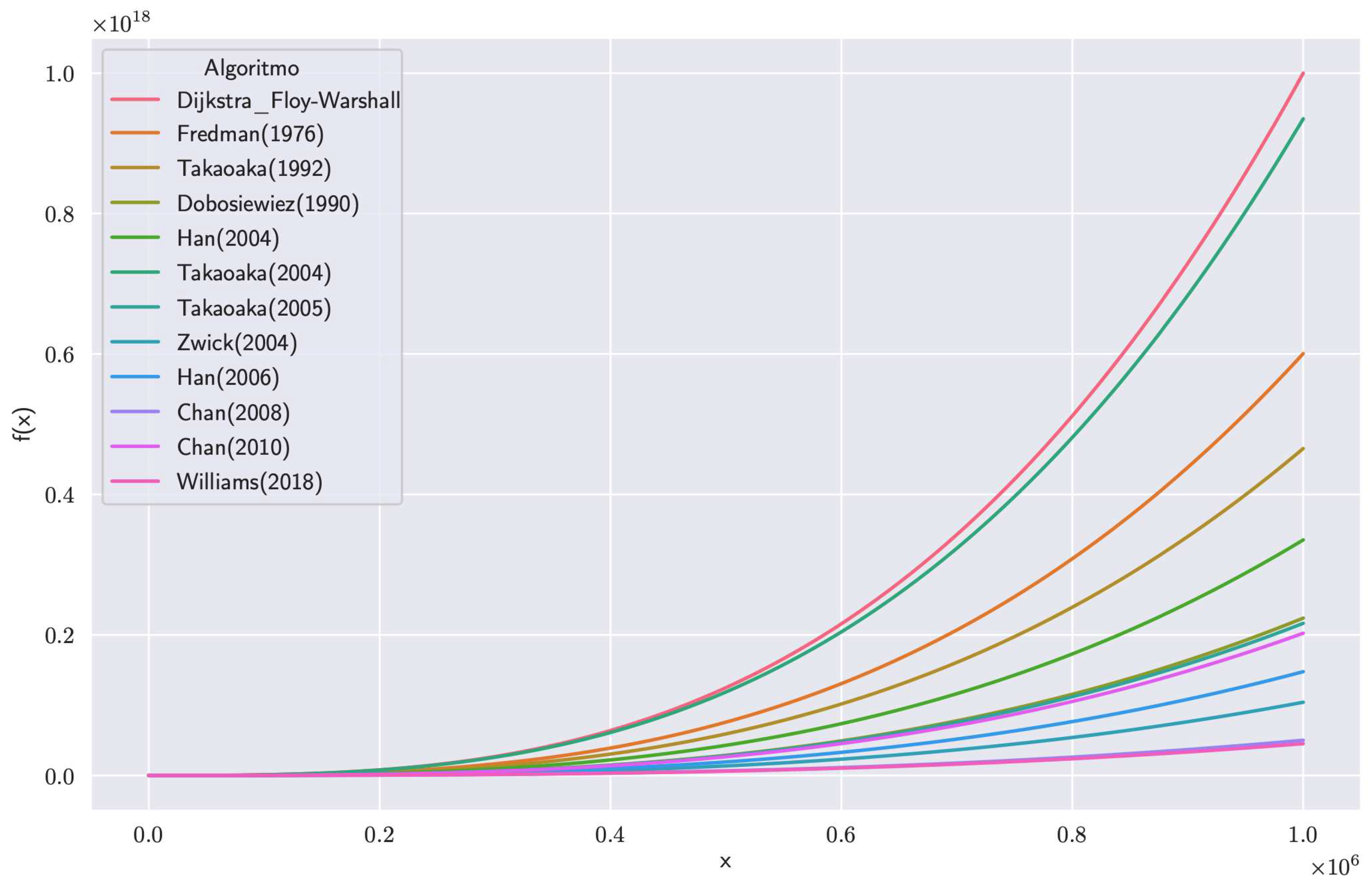
Figure 2.
The DIS-C algorithm flow diagram.
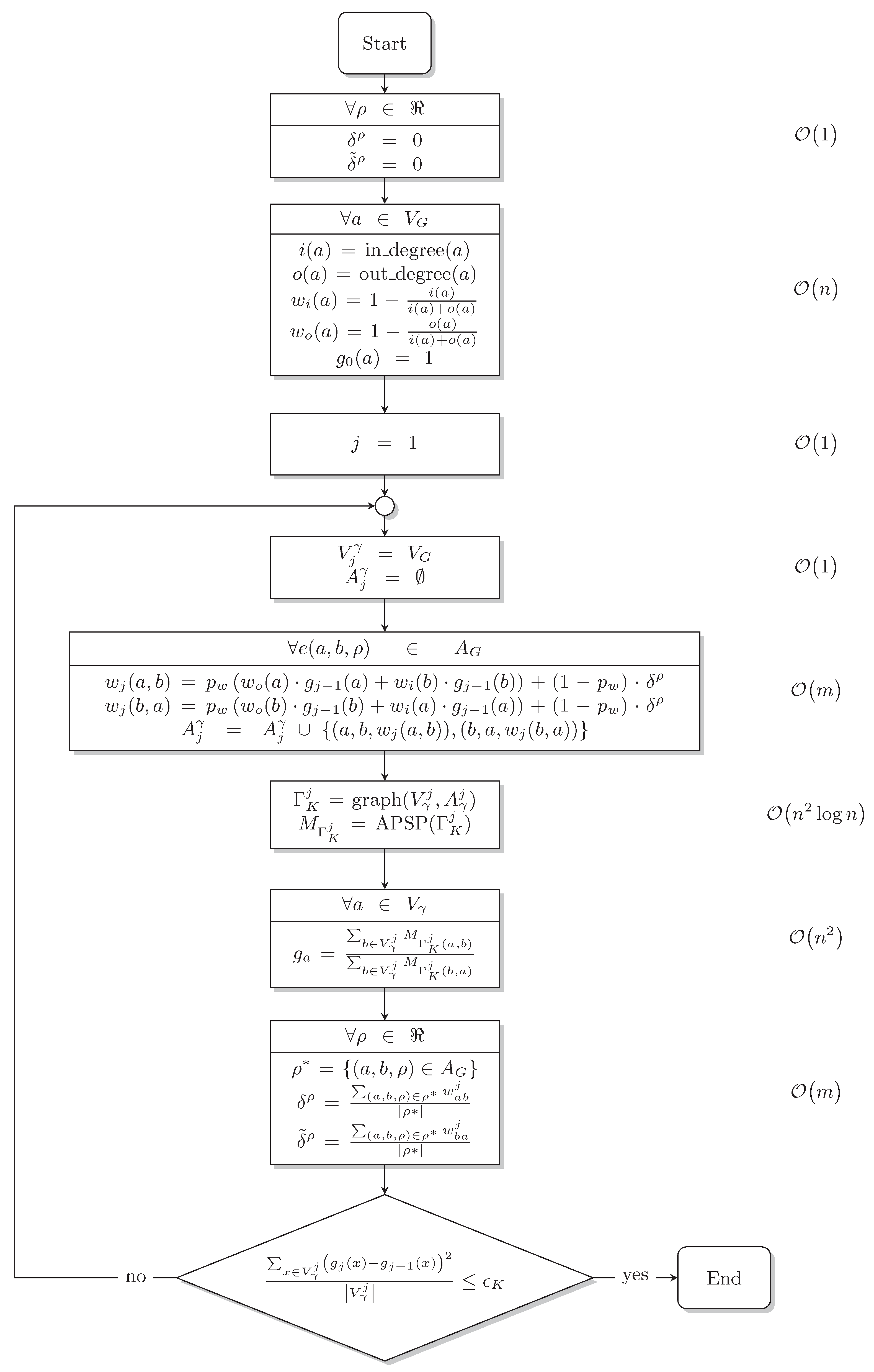
Figure 3.
The DIS-C algorithm flow diagram.
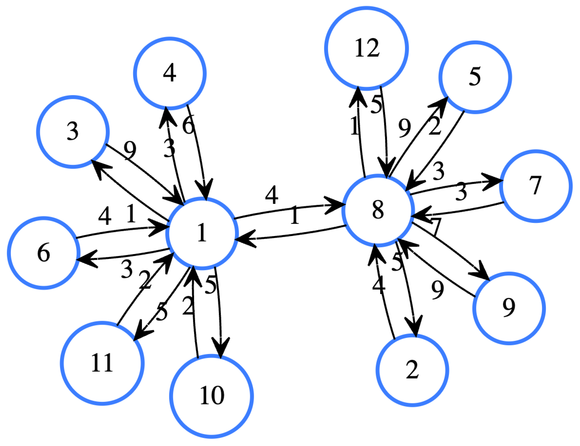
Figure 4.
Example of the pruned Dijkstra. The red vertices denote the execution root, the green ones denote those visited and added to the coverage, and the gray ones are the roots.
Figure 4.
Example of the pruned Dijkstra. The red vertices denote the execution root, the green ones denote those visited and added to the coverage, and the gray ones are the roots.
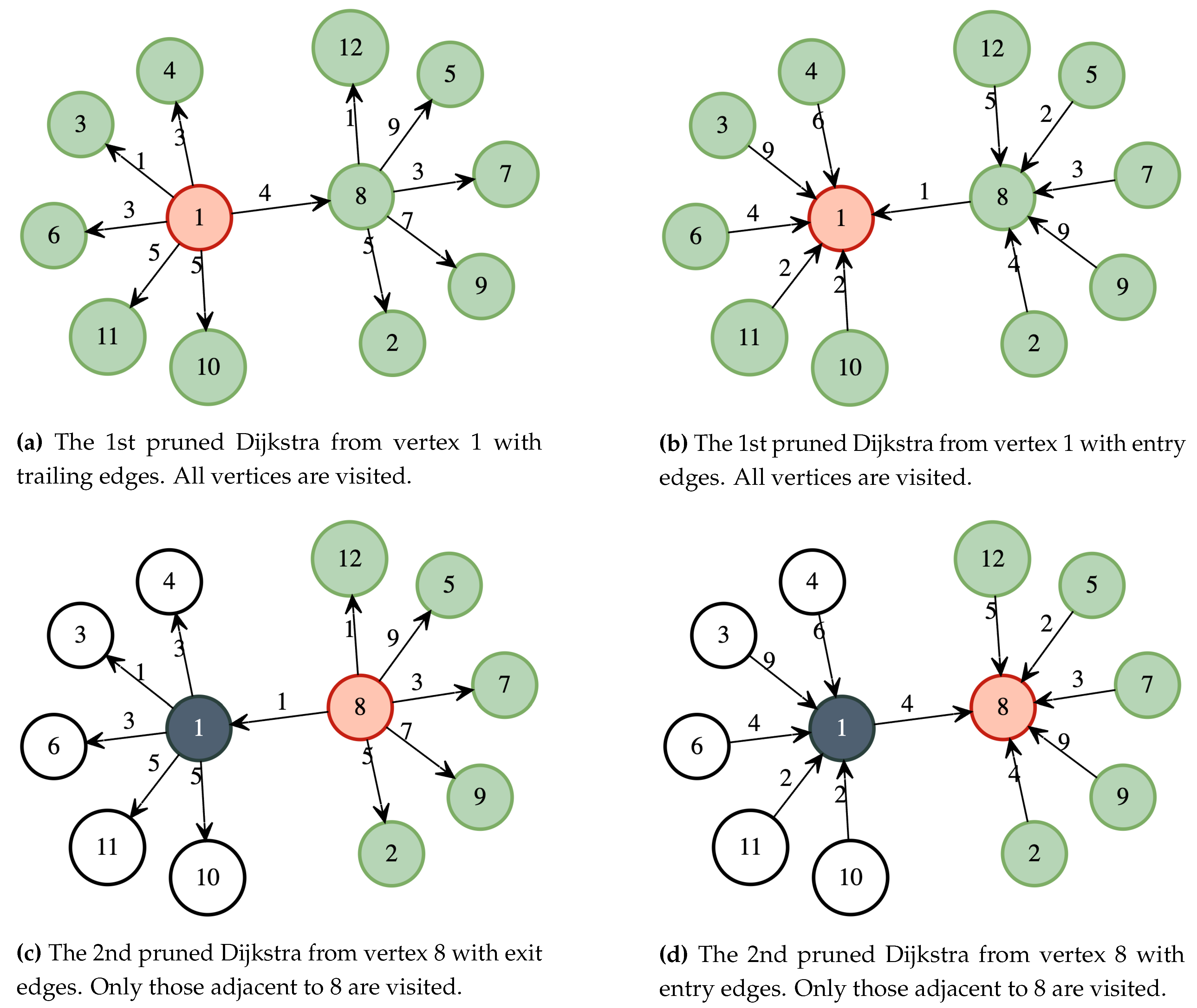
Figure 5.
Sketches example. The red vertices denote the execution root, and the green ones represent those that are visited.
Figure 5.
Sketches example. The red vertices denote the execution root, and the green ones represent those that are visited.
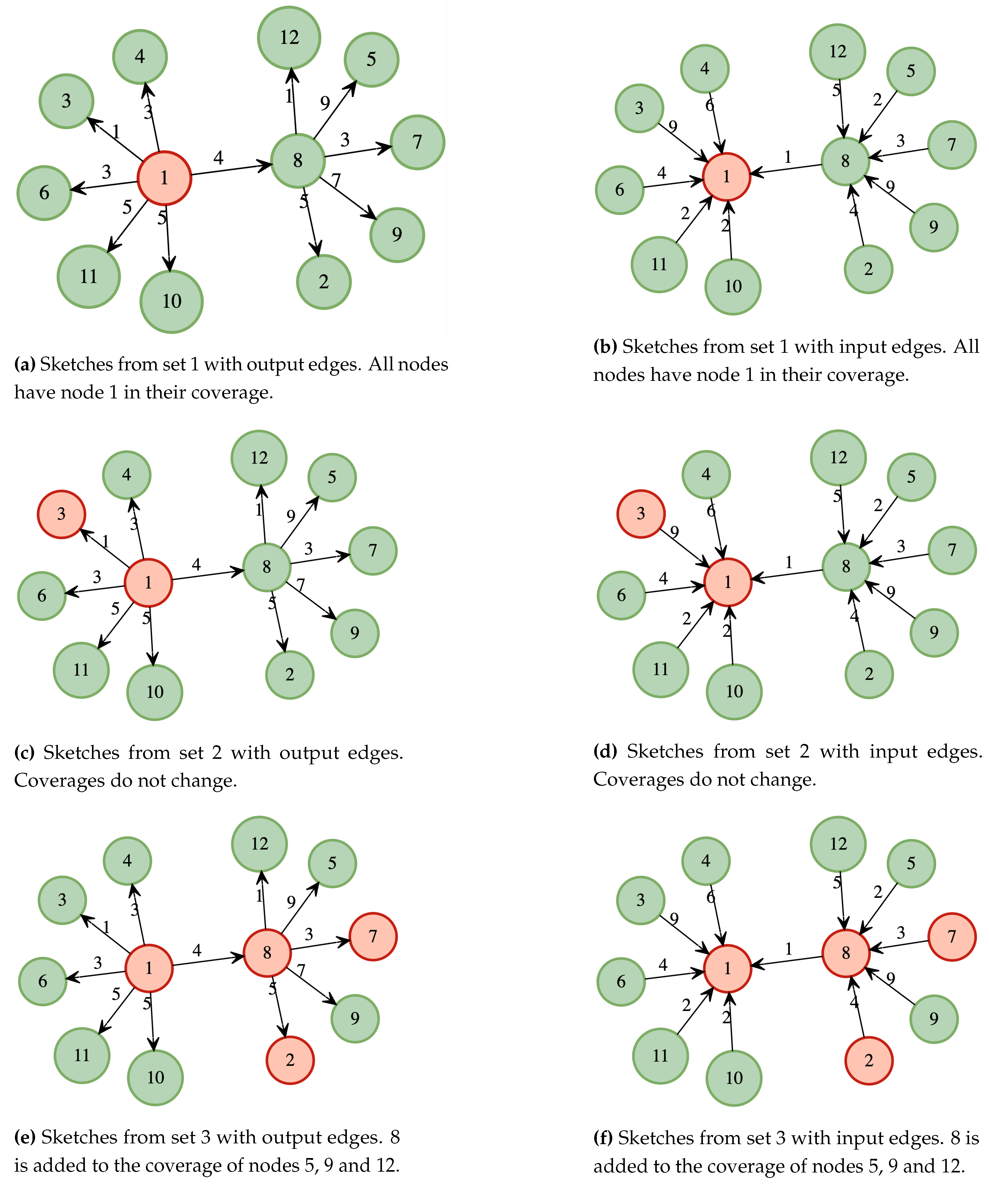
Figure 6.
The DIS-C runtime with the algorithms: Dijkstra,the pruned Dijkstra and Sketches.
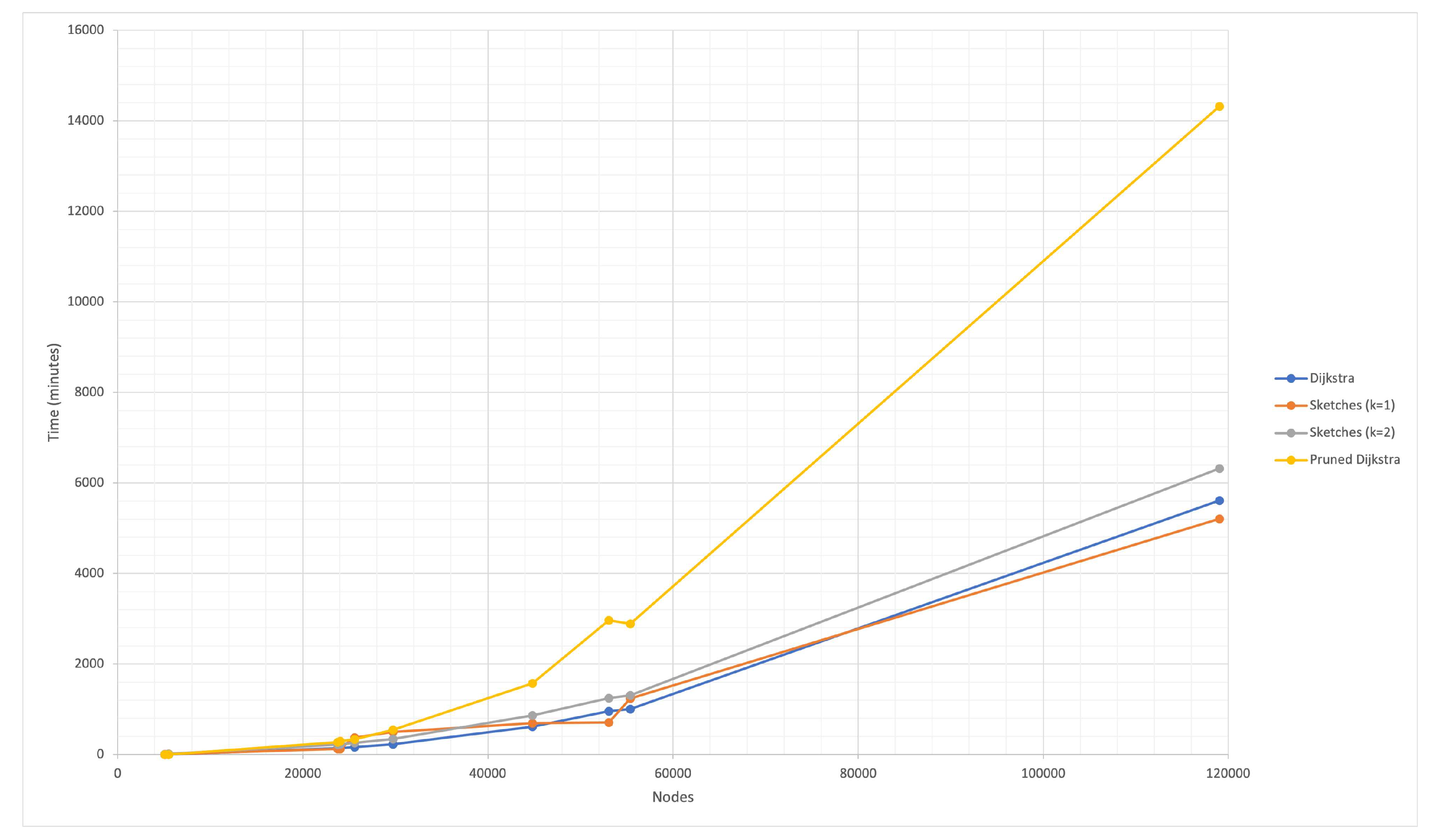
Figure 7.
Construction time (offline) and query time (inline). .
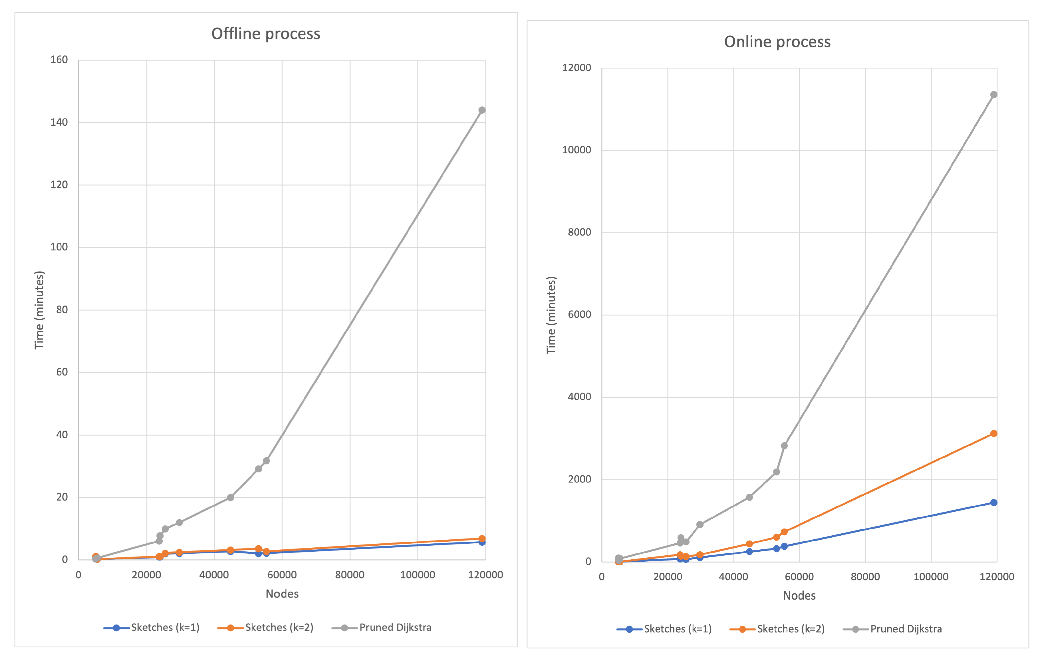
Figure 8.
Simple DIS-C runtime with the algorithms: Dijkstra, the pruned Dijkstra simple, and Sketches simple.
Figure 8.
Simple DIS-C runtime with the algorithms: Dijkstra, the pruned Dijkstra simple, and Sketches simple.
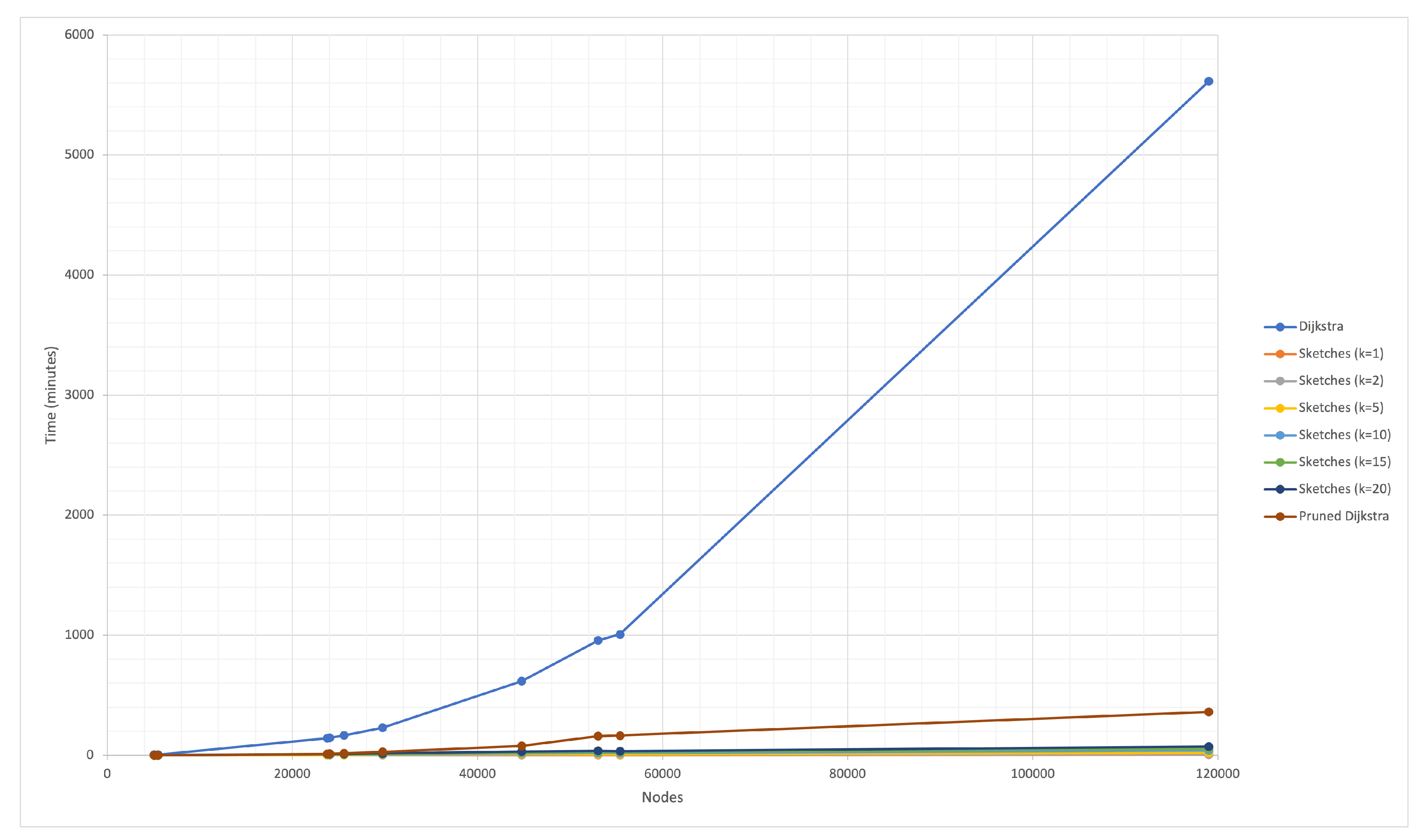
Figure 9.
The Pearson correlation matrix of the MC30 dataset.
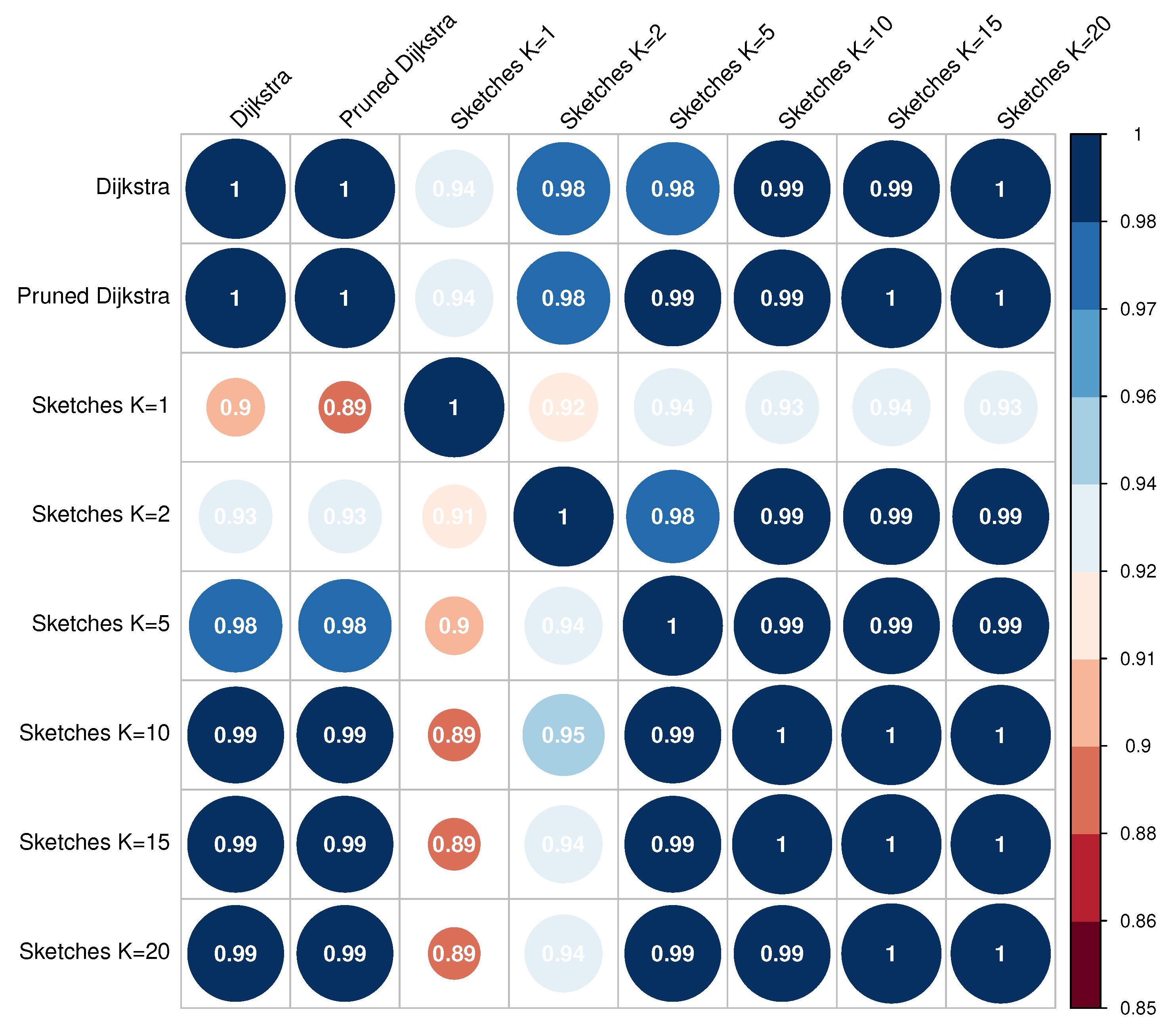
Figure 10.
The Spearman correlation matrix of the MC30 dataset.
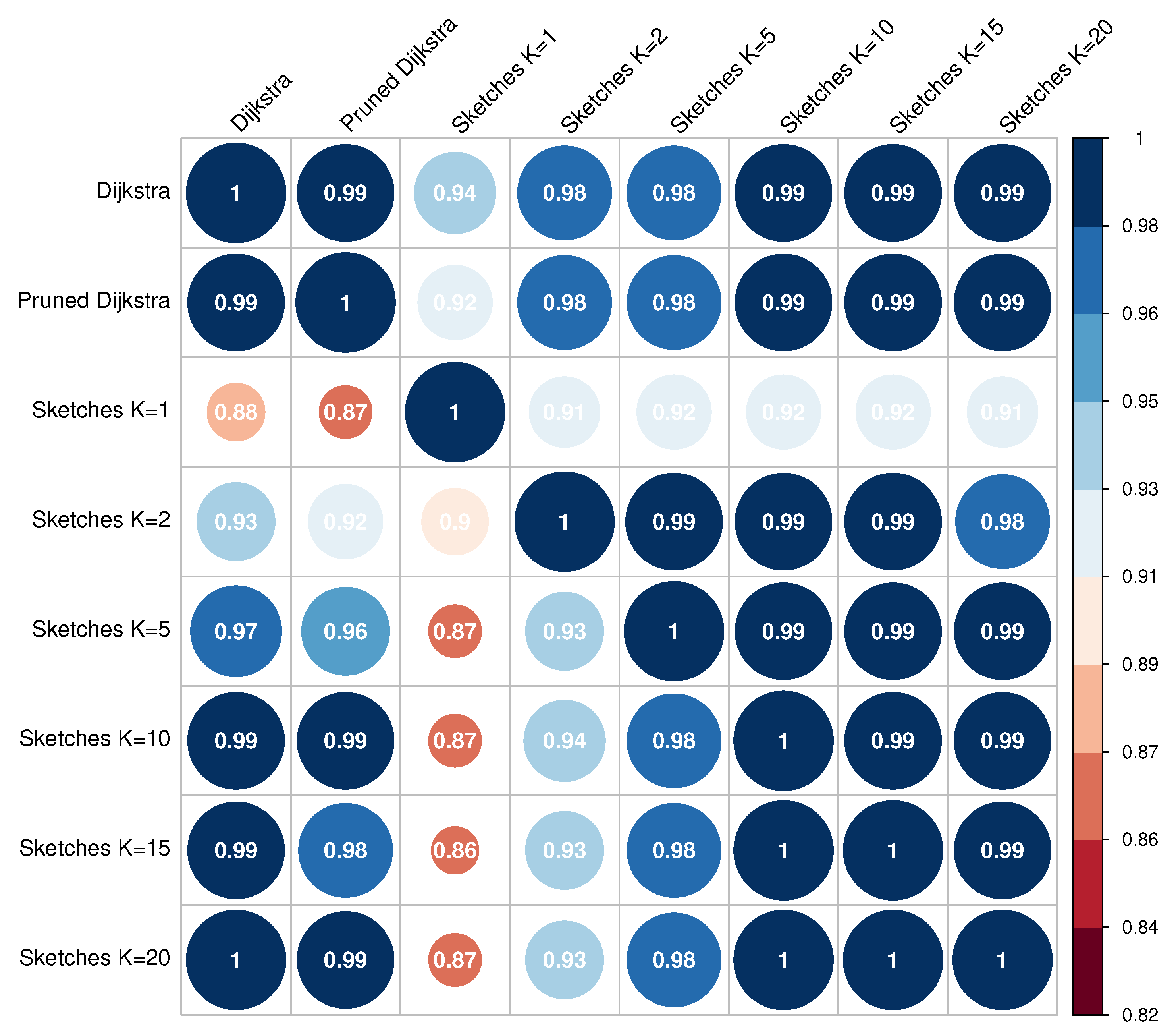

Table 1.
Edge counting-based methods
| Reference | Expression | Description |
|---|---|---|
| Rada et al. (1989) [14] | length of path from a to b | |
| Wu and Palmer (1994) [15] | a and b are concepts within the hierarchy, c is a less common super concept of a and b. is the number of nodes in the path from a to c, is the number of nodes in the path from b to c and is the number of nodes in the path from c to the root of the hierarchy. | |
| Hirst and Stonge (1995) [16] | C and K are constants, is the length of the shortest path between a and b, and is the number of times the path changes direction. | |
| Li et al. (2003) [18] | is the length of the shortest path between a and b, h is the minimum depth of LCS (the more specific concept that is an ancestor of a and b) in the hierarchy, and are parameters that scale the contribution of the shortest path length and depth, respectively. | |
| Shenoy et al. (2012) [19] | L is the shortest distance between a and b calculated taking into account the direction of the edges. Each vertical direction is given a value of 1; each time it changes direction, one more is added. N is the depth of the entire tree. and are the distances from the root to the concept a and b respectively. is 1 for neighboring concepts and 0 for the others |
Table 2.
Information content-based methods
| Reference | Expression | Description |
|---|---|---|
| Resnik (1995) [24] | Based on the notion of the LCS (Least Common Subsumer), if the terms share an LCS, then the IC is calculated from it. | |
| Jiang and Conrath (1997) [26] | It focuses on determining the link strength of an edge connecting a parent node with a child node. These taxonomic links between concepts are reinforced by the difference between the IC of a concept and its LCS. | |
| Gao et al. (2015) [27] | Where is a constant and is the set of senses of the concept x. | |
| Jiang et al. (2017) [28] | Where is the set of hyponyms for a, is the set of pages in category c and is the set of categories. | |
| The second proposed approach is the combination of the IC by using the category structure and the extension of ontology-based methods. | ||
| Generalization of the Zhou et al. (2008) [29] approach. Where is an adjustment factor for the weight of the two characteristics involved in the IC calculation, is the depth of the leaf a, and is the maximum depth of a leaf. | ||
| Generalization of the Sanchez et al. (2011) [30] approach. Where is the set of leaves of a in the category hierarchy, is the set of hypernyms, and is the maximum number of leaves in the hierarchy. |
Table 3.
Analytical algorithm runtime for APSP
| Reference | Year | |
|---|---|---|
| Dijkstra/Floyd–Warshall | 1959/1962 | |
| Fredman (1976) [50] | 1976 | |
| Takaoka (1992) [51] | 1991 | |
| Dobosiewicz (1990) [52] | 1990 | |
| Han (2004) [53] | 2004 | |
| Takaoka (2004) [54] | 2004 | |
| Takaoka (2005) [55] | 2005 | |
| Zwick (2004) [56] | 2004 | |
| Chan (2008) [57] | 2005 | |
| Han (2006) [58] | 2006 | |
| Chan (2010) [41] | 2007 | |
| Williams (2018) [44] | 2014 |
Table 4.
Dataset for evaluation procedure
| Dataset | Content | Type | Word pairs |
|---|---|---|---|
| MC30 [74] | Nouns | Similarity | 30 |
| RG65 [75] | Nouns | Similarity | 65 |
| PS [76] | Nouns | Similarity | 65 |
| Agirre201 [77] | Nouns | Similarity | 201 |
| SimLex665 [78] | Nouns | Similarity | 665 |
| MTurk771 [79] | Nouns | Relation | 771 |
| MTurk287 [80] | Nouns | Relation | 287 |
| WS245Rel [81] | Nouns | Relation | 245 |
| Rel122 [82] | Nouns | Relation | 122 |
| SCWS [83] | Nouns | Relation | 1994 |
Table 5.
Total nodes and edges of the underlying graphs of the datasets.
| Dataset | Word pairs | Nodes | Edges |
|---|---|---|---|
| Dijkstra/Floyd–Warshall | 1959/1962 | ||
| MC30 | 30 | 5,496 | 9583 |
| RG65 | 65 | 5,080 | 9271 |
| PS | 65 | 5,080 | 9271 |
| Agirre201 | 201 | 29,738 | 75,120 |
| SimLex665 | 665 | 44,798 | 138,122 |
| MTurk771 | 771 | 55,403 | 185,523 |
| MTurk287 | 287 | 25,576 | 58,637 |
| WS245Rel | 245 | 24,029 | 56,983 |
| Rel122 | 122 | 23,775 | 58,322 |
| SCWS | 1,994 | 53,052 | 183,366 |
| All | 4,445 | 119,034 | 818,788 |
Table 6.
The Pearson correlation of all datasets in the direction
| Algorithm | MC30 | RG | PS | Agirre | SimLex | MTurk | MTurk | WSRel | Rel | SCWS | All | Avg. |
|---|---|---|---|---|---|---|---|---|---|---|---|---|
| Dijkstra | 1.000 | 1.000 | 1.000 | 1.000 | 1.000 | 1.000 | 1.000 | 1.000 | 1.000 | 1.000 | 1.000 | 1.000 |
| Pruned Dijkstra | 1.000 | 1.000 | 1.000 | 1.000 | 1.000 | 1.000 | 1.000 | 1.000 | 1.000 | 1.000 | 0.997 | 1.000 |
| Sketches k=1 | 0.940 | 0.853 | 0.862 | 0.733 | 0.762 | 0.605 | 0.864 | 0.720 | 0.841 | 0.815 | 0.745 | 0.795 |
| Sketches k=2 | 0.977 | 0.947 | 0.961 | 0.870 | 0.813 | 0.731 | 0.888 | 0.842 | 0.922 | 0.898 | 0.802 | 0.877 |
| Sketches k=5 | 0.985 | 0.984 | 0.978 | 0.923 | 0.897 | 0.881 | 0.937 | 0.921 | 0.953 | 0.944 | 0.899 | 0.937 |
| Sketches k=10 | 0.991 | 0.979 | 0.995 | 0.961 | 0.955 | 0.931 | 0.967 | 0.959 | 0.976 | 0.971 | 0.942 | 0.966 |
| Sketches k=15 | 0.993 | 0.996 | 0.991 | 0.980 | 0.972 | 0.959 | 0.971 | 0.971 | 0.983 | 0.982 | 0.957 | 0.978 |
| Sketches k=20 | 0.996 | 0.992 | 0.994 | 0.983 | 0.974 | 0.971 | 0.979 | 0.975 | 0.989 | 0.986 | 0.972 | 0.983 |
Table 7.
The Pearson correlation of all datasets in the direction
| Algorithm | MC | RG | PS | Agirre | SimLex | MTurk | MTurk | WSRel | Rel | SCWS | All | Avg. |
|---|---|---|---|---|---|---|---|---|---|---|---|---|
| Dijkstra | 1.000 | 1.000 | 1.000 | 1.000 | 1.000 | 1.000 | 1.000 | 1.000 | 1.000 | 1.000 | 1.000 | 1.000 |
| Sketches k=1 | 0.897 | 0.777 | 0.877 | 0.734 | 0.722 | 0.562 | 0.862 | 0.757 | 0.857 | 0.793 | 0.733 | 0.779 |
| Sketches k=2 | 0.932 | 0.961 | 0.956 | 0.893 | 0.806 | 0.725 | 0.890 | 0.827 | 0.879 | 0.896 | 0.795 | 0.869 |
| Sketches k=5 | 0.979 | 0.984 | 0.981 | 0.909 | 0.893 | 0.865 | 0.946 | 0.936 | 0.947 | 0.945 | 0.897 | 0.935 |
| Sketches k=10 | 0.987 | 0.991 | 0.992 | 0.963 | 0.952 | 0.944 | 0.960 | 0.945 | 0.979 | 0.967 | 0.939 | 0.965 |
| Sketches k=15 | 0.992 | 0.998 | 0.994 | 0.968 | 0.971 | 0.958 | 0.975 | 0.966 | 0.978 | 0.980 | 0.960 | 0.976 |
| Sketches k=20 | 0.995 | 0.996 | 0.997 | 0.979 | 0.971 | 0.972 | 0.980 | 0.983 | 0.984 | 0.988 | 0.972 | 0.983 |
Table 8.
The Spearman correlation of all datasets in the direction
| Algorithm | MC | RG | PS | Agirre | SimLex | MTurk | MTurk | WSRel | Rel | SCWS | All | Avg. |
|---|---|---|---|---|---|---|---|---|---|---|---|---|
| Dijkstra | 1.000 | 1.000 | 1.000 | 1.000 | 1.000 | 1.000 | 1.000 | 1.000 | 1.000 | 1.000 | 1.000 | 1.000 |
| Pruned Dijkstra | 1.000 | 1.000 | 1.000 | 1.000 | 1.000 | 1.000 | 1.000 | 1.000 | 1.000 | 1.000 | 0.968 | 0.997 |
| Sketches k=1 | 0.938 | 0.876 | 0.858 | 0.702 | 0.742 | 0.605 | 0.843 | 0.671 | 0.799 | 0.831 | 0.736 | 0.782 |
| Sketches k=2 | 0.977 | 0.944 | 0.959 | 0.823 | 0.804 | 0.729 | 0.855 | 0.821 | 0.900 | 0.906 | 0.807 | 0.866 |
| Sketches k=5 | 0.978 | 0.978 | 0.984 | 0.911 | 0.887 | 0.876 | 0.925 | 0.907 | 0.950 | 0.954 | 0.897 | 0.931 |
| Sketches k=10 | 0.987 | 0.981 | 0.991 | 0.941 | 0.955 | 0.931 | 0.963 | 0.946 | 0.973 | 0.978 | 0.942 | 0.962 |
| Sketches k=15 | 0.987 | 0.993 | 0.985 | 0.968 | 0.971 | 0.969 | 0.963 | 0.960 | 0.980 | 0.986 | 0.954 | 0.974 |
| Sketches k=20 | 0.989 | 0.988 | 0.991 | 0.973 | 0.979 | 0.978 | 0.976 | 0.961 | 0.985 | 0.990 | 0.965 | 0.980 |
Table 9.
The Spearman correlation of all datasets in the direction
| Algorithm | MC | RG | PS | Agirre | SimLex | MTurk | MTurk | WSRel | Rel | SCWS | All | Avg. |
|---|---|---|---|---|---|---|---|---|---|---|---|---|
| Dijkstra | 1.000 | 1.000 | 1.000 | 1.000 | 1.000 | 1.000 | 1.000 | 1.000 | 1.000 | 1.000 | 1.000 | 1.000 |
| Pruned Dijkstra | 1.000 | 1.000 | 1.000 | 1.000 | 1.000 | 1.000 | 1.000 | 1.000 | 1.000 | 1.000 | 0.969 | 0.997 |
| Sketches k=1 | 0.875 | 0.826 | 0.843 | 0.735 | 0.700 | 0.573 | 0.823 | 0.693 | 0.817 | 0.807 | 0.732 | 0.766 |
| Sketches k=2 | 0.925 | 0.921 | 0.932 | 0.859 | 0.816 | 0.733 | 0.876 | 0.764 | 0.835 | 0.902 | 0.803 | 0.851 |
| Sketches k=5 | 0.972 | 0.970 | 0.961 | 0.898 | 0.884 | 0.866 | 0.920 | 0.906 | 0.936 | 0.953 | 0.896 | 0.924 |
| Sketches k=10 | 0.991 | 0.980 | 0.985 | 0.953 | 0.950 | 0.947 | 0.945 | 0.928 | 0.969 | 0.974 | 0.938 | 0.960 |
| Sketches k=15 | 0.991 | 0.990 | 0.981 | 0.959 | 0.974 | 0.960 | 0.961 | 0.952 | 0.969 | 0.984 | 0.958 | 0.971 |
| Sketches k=20 | 0.996 | 0.985 | 0.990 | 0.973 | 0.971 | 0.977 | 0.971 | 0.975 | 0.982 | 0.991 | 0.966 | 0.980 |
Table 10.
Harmonic values of the correlations
| Algorithm | MC | RG | PS | Agirre | SimLex | MTurk | MTurk | WSRel | Rel | SCWS | All | Avg. |
|---|---|---|---|---|---|---|---|---|---|---|---|---|
| Dijkstra | 1.00 | 1.00 | 1.00 | 1.00 | 1.00 | 1.00 | 1.00 | 1.00 | 1.00 | 1.00 | 0.0 | 1.00 |
| Pruned Dijkstra | 1.00 | 1.00 | 1.00 | 1.00 | 1.00 | 1.00 | 1.00 | 1.00 | 1.00 | 1.00 | 0.0 | 1.00 |
| Sketches k=1 | 0.94 | 0.86 | 0.86 | 0.72 | 0.75 | 0.61 | 0.85 | 0.69 | 0.82 | 0.82 | 0.0 | 0.79 |
| Sketches k=2 | 0.98 | 0.95 | 0.96 | 0.85 | 0.81 | 0.73 | 0.87 | 0.83 | 0.91 | 0.90 | 0.0 | 0.88 |
| Sketches k=5 | 0.98 | 0.98 | 0.98 | 0.92 | 0.89 | 0.88 | 0.93 | 0.91 | 0.95 | 0.95 | 0.0 | 0.94 |
| Sketches k=10 | 0.99 | 0.98 | 0.99 | 0.95 | 0.95 | 0.93 | 0.97 | 0.95 | 0.97 | 0.97 | 0.0 | 0.97 |
| Sketches k=15 | 0.99 | 0.99 | 0.99 | 0.97 | 0.97 | 0.96 | 0.97 | 0.97 | 0.98 | 0.98 | 0.0 | 0.98 |
| Sketches k=20 | 0.99 | 0.99 | 0.99 | 0.98 | 0.98 | 0.97 | 0.98 | 0.97 | 0.99 | 0.99 | 0.0 | 0.98 |
Disclaimer/Publisher’s Note: The statements, opinions and data contained in all publications are solely those of the individual author(s) and contributor(s) and not of MDPI and/or the editor(s). MDPI and/or the editor(s) disclaim responsibility for any injury to people or property resulting from any ideas, methods, instructions or products referred to in the content. |
© 2023 by the authors. Licensee MDPI, Basel, Switzerland. This article is an open access article distributed under the terms and conditions of the Creative Commons Attribution (CC BY) license (http://creativecommons.org/licenses/by/4.0/).
Copyright: This open access article is published under a Creative Commons CC BY 4.0 license, which permit the free download, distribution, and reuse, provided that the author and preprint are cited in any reuse.


