
Submitted:
09 October 2023
Posted:
11 October 2023
You are already at the latest version
Abstract
The main aim of this study is to predict whether the type of breast cancer is “benign” or “malignant” by classical generalized linear model (GLM) approach and an extended family of GLM called generalized linear mixed model (GLMM) approach for binomially distributed response variable with binary link functions. In this study, an advanced statistical modeling approach based on the GLMM to the traditional statistical modeling approach based on the GLM for binomially distributed response variable with various binary link functions is proposed to investigate the relationships between the “malignant or benign diagnosis of the BC in patients” and “nine attributes” of 699 BC diagnosed patients. This study also focuses on the statistical significance of the accurate classification of the BC diagnosed patients in cancer studies in medicine in “benign” or “malignant” type based on the WBC dataset. In this study, the superiority of the GLMM approach over the GLM approach for the binary response variable especially belonging to the WBC dataset is emphasized in the field of cancer diagnosis in medicine. Also the importance and the power of the IC and performance metrics as the goodness-of-fit test statistics are strongly emphasized for accurate statistical inferences from the “best” fitted model. In this study, from the main findings, the best fitted model among the GLM and GLMM approaches for the binary response variable is determined as the GLMM under “logit” link function with “id” random effect with the most statistically significant odds of the occurance of the BC being “malignant” as 7.9104, 5.6888, 5.6643, 4.9842, 4.1212, 2.0679, 1.8755, and 1.3970 times more than being “benign” for every one-unit increase in the quantities of “clump thickness”, “bland chromatin”, “mitoses”, “bare nuclei”, “cell shape”, “marginal adhesion”, “epithelial cell size”, and “cell size”, respectively.
Keywords:
Generalized linear mixed model
; Wisconsin breast cancer data
; logit
; probit
; cloglog
; cauchit link functions
; random effect
1. Introduction
The most importance of “breast cancer (BC)” taken in this study is being the fourth common seen cancer type and one of the most leading causes of mortality all over the world with 700.147 number of deaths belonging to 200 countries in the world in 2019 (Aalaei et al. [1], Kadhim and Kamil [2], Roser and Ritchie [3], Our World in Data [4], Desantis et al. [5]). Breast cancer mortality rates among deaths caused by all cancer types according to the 200 countries in the world in 2019 are illustrated in Figure 1.
As can be seen from Figure 1, among deaths caused by all cancer types belonging to the 200 countries in the world in 2019, the percentage of deaths from breast cancer is concentrated between approximately 6% and 15%. Five countries with the highest mortality rates from breast cancer are Solomon Islands with 24.48%, Papua New Guinea with 24.16%, Pakistan with 19.84%, Fiji with 18.99%, and Nigeria with 17.55%, respectively. On the other hand, five countries with the least mortality rates from breast cancer are Taiwan with 4.21%, South Korea with 4.02%, Japan with 3.72%, China with 3.64%, and Mongolia with 2.41%, respectively.
There are many studies in the literature on the popularly used “Wisconsin Breast Cancer (WBC) Dataset”, which is still very up-to-date and examined through many different statistical and machine learning methods. A detailed review of the wide variety of related studies done on the WBC dataset can be given as follows;
Jain and Abraham [6] investigated performances of fuzzy classification methods to approach a high classification rate in detecting BC using the WBC dataset. Karabatak and İnce [7] proposed an integrated neural network and association rules approach for the classification of BC using the WBC dataset. Fallahi and Jafari [8] showed accuracy of the classifiers based on Bayesian network approach to detect BC using the WBC dataset. Kumar et al. [9] established classification models for predicting BC by data mining methods using the WBC dataset. Borges [10] employed machine learning techniques based on Bayesian approach to detect BC using the WBC dataset. Aalaei et al. [1] emphasized superiority of genetic algorithm in terms of accuracy, specificity, and sensitivity features of different classifiers on the WBC dataset for the aim of disease diagnosis of breast cancer. Dubey et al. [11] applied k-means clustering algorithm for diagnosing BS using the WBC dataset. Banerjee et al. [12] constructed ensemble learning techniques as a machine learning study for the classification of BC based on the WBC dataset. Alshayeji et al. [13] used artificial neural network (ANN) model in the early diagnosis of breast cancer (BC) depending on the WBC dataset and evaluated accuracy, sensitivity, and specificity of their proposed ANN models. Kadhim and Kamil [2] compared the performances of machine learning classifiers in terms of some criteria.
Mumtaz et al. [14], Sarvestani et al. [15], Marcano-Cedeño et al. [16], Salama et al. [17], Shajahaan et al. [18], Vig [19], Sivakami and Saraswathi [20], Kumari and Singh [21], Obaid et al. [22], Sultana and Jilani [23], Mohammed et al. [24], and Mushtaq et al. [25] applied neural network models; data mining techniques; artificial neural network; multi-classifiers; data mining techniques; neural networks; DT - SVM hybrid model; KNN and SVM classifiers; machine learning techniques; multi-class classifiers; machine learning methods; k-nearest neighbor classification methods to the WBC dataset in the prediction, classification, and diagnosis of the BC in terms of various features such as accuracy, specificity, and sensitivity.
Sultana and Jilani [23], MurtiRawat et al. [26], Seddik and Shawky [27], Mathew and Kumar [28], Li and Chen [29], Magboo and Magboo [30], Haziemeh et al. [31], Mathew [32], Basunia et al. [33], Al-Azzam and Shatnawi [34], Khairunnahar et al. [35], Islam et al. [36], Mushtaq et al. [37], Hossin et al. [38], and Rekha and Vinoci [39] used logistic regression in the prediction of BC to classify types of patients with diagnosis of BC as “benign” or “malignant”.
As seen from the literature review, many authors focused on accurate classification of the WBC dataset by machine learning and data mining techniques with various classifiers and neural network approaches. The most common purpose of these studies on the WBC dataset in the literature is to apply machine learning algorithms in predicting and diagnosing BC due to the specificity, sensitivity, precision, and accuracy criteria in BC diagnosis based on the WBC dataset.
In the light of the studies given in the literature above and also in addition to the literature, in this study, an advanced statistical modeling approach based on the generalized linear mixed model (GLMM) to the traditional statistical modeling approach based on the generalized linear model (GLM) for binomially distributed response variable with various binary link functions is proposed to investigate the relationships between the “malignant or benign diagnosis of the BC in patients” and “nine attributes” of 699 BC diagnosed patients. This study also focuses on the statistical significance of the accurate classification of the BC diagnosed patients in cancer studies in medicine in “benign” or “malignant” type based on the WBC dataset.
This study consists of four sections. In the first section, “Wisconsin Breast Cancer (WBC) Dataset” and related studies on WBC dataset in the literature are introduced. In the second section, attributes of the WBC dataset are briefly described and the GLMM approach as the method used in this study is given in details. In the third and fourth sections, empirical results and discussions, as well as conclusions based on the examination of the WBC dataset with the GLMM approach, are presented in detail.
2. Materials and Methods
In this section, “Wisconsin Breast Cancer (WBC) Dataset” is introduced and attributes of the WBC dataset are briefly described and then the GLMM approach for binary response variable as the method used in this study is given in details.
2.1. Materials
Dr. William H. Wolberg from the University of Wisconsin Hospitals in Madison examined the samples taken from the patients for the diagnosis of breast cancer (BC) under the microscope. Then, these samples were examined under the microscope and numbers from 1 to 10 were assigned to 9 different quantities related to the BC including “clump thickness”, “cell size”, “cell shape”, “marginal adhesion”, “epithelial cell size”, “bare nuclei”, “bland chromatin”, "normal nucleoli", and “mitoses” for each sample point in the WBC dataset (Mangasarian and Wolberg [40], Wolberg and Mangasarian [41], Wolberg et al. [42], Bennett and Mangasarian [43]).
WBCD dataset available on 15 July 1992 consisted of eight groups and totally 699 sample points which were 367 sample points from group 1 (January 1989), 70 sample points from group 2 (October 1989), 31 sample points from group 3 (February 1990), 17 sample points from group 4 (April 1990), 48 sample points from group 5 (August 1990), 49 sample points from group 6 (January 1991), 31 sample points from group 7 (June 1991), and 86 sample points from group 8 (November 1991). 458 benign (B) sample points and 241 malignant (M) sample points were determined at totally 699 sample points according to these eight groups in the WBDC dataset (Wolberg [44]).
In this section of this study, “readxl”, “stats” and “ggplot” packages in the RStudio programme are used both in obtaining descriptive statistics and data visualization stages of the WBC dataset (Wickham [45], Team et al. [46], Wickham et al. [47]). The quantity of "normal nucleoli" is removed due to its inconsistent parameter estimates in the advanced statistical models performed in this study. Descriptive statistics for the 699 sample points according to their “benign” or “malignant” status of the remaining eight different quantities related to the BC are given in Table 1.
Descriptive statistics for the WBC dataset given in Table 1 are also graphically demonstrated in Figure 2 for a better visual understanding.
In Figure 2, green and red bars are seperately given for the eight quantities belonging to the “benign” and “malignant” samples, respectively. The boxes in the middle of each bar show average (mean) values of the related quantities, and the lower and upper values show the mean valuesstandard deviation values, respectively. Among the quantities determined for “benign” samples, the highest and the lowest mean values are determined for the “clump thickness” and “mitoses” with 2.6563, and 1.0633, respectively. The lowest lenghts of the bars calculated as 2standard deviation for the “benign” and “malignant” samples is on “mitoses” with 1.004, and on “bland chromatin” with 4.5478, respectively. On the other hand, the highest lenghts of the bars for the “benign” and “malignant” samples is on “clumb thickness” with 3.3486, and on “marginal adhesion” with 6.4210, respectively. As can be seen from Table 1 and Figure 2, descriptive statistics for the “malignant” samples are significantly higher in terms of both their averages and standard deviations compared to the “benign” samples.
As a more detailed version of the descriptive statistics given in Table 1, descriptive statistics of totally 699 sample points according to their “benign” and “malignant” status, eight different groups, and eight different quantities are given in Table 2.
As can be seen from Table 2, the highest values of the means and the standard deviations among the 699 sample points detected as "benign" according to their eight quantities in eight groups are determined on "clumb thickness" with mean values 2.6750, 2.7544, 3.6364, 4.2857, 3.1389, 3.4250, 3.7647, and 2.8889; and also standard deviation values 1.7333, 1.5616, 1.6197, 1.3260, 1.5703, 1.5340, 1.5219, and 1.5883, respectively. On the other hand, the highest values of means among the sample groups detected as “malignant” according to eight quantities are determined on “bare nuclei” with mean value 7.6168 in group 1, “clumb thickness” with mean value 8.3077 in group 2, “clumb thickness” with mean value 8.1111 in group 3, “bland chromatin” with mean value 8.6667 in group 4, “bare nuclei” with mean value 8.0833 in group 5, “bare nuclei” with mean value 8.0000 in group 6, “bland chromatin” with mean value 7.5714 in group 7, and “cell size” with mean value 8.8571 in group 8.
The highest values of standard deviations among the sample groups detected as “malignant” according to eight quantities are determined on “marginal adhesion” with standard deviation value 3.2157 in group 1, “bare nuclei” with standard deviation value 3.3874 in group 2, “clumb thickness” with standard deviation value 2.9768 in group 3, “mitoses” with standard deviation value 5.1962 in group 4, “marginal adhesion” with standard deviation value 3.5633 in group 5, “marginal adhesion” with standard deviation value 3.3082 in group 6, “bare nuclei” with standard deviation value 3.8381 in group 7, and “bare nuclei” with standard deviation value 3.2148 in group 8.
The frequencies and relative frequencies of eight quantities taken values from 1-10 according to “benign”, “malignant”, and both status of these sample groups are separately given in Table 3.
As can be seen from Table 3, according to the “benign” and “malignant” status of the samples, the frequencies of the “clump thickness”, “cell size”, “cell shape”, “marginal adhesion”, “epithelial cell size”, “bare nuclei”, “bland chromatin”, and “mitoses” are determined as at most of values at 1 with 142 (31%), at 1 with 380 (82.97%), at 1 with 351 (76.64%), at 1 with 375 (81.88%), at 2 with 363 (79.26%), at 1 with 387 (84.50%), at 2 with 159 (34.72%), and at 1 with 445 (97.16%), ; and also at 10 with 69 (28.63%), at 10 with 67 (27.80%), at 10 with 58 (24.07%), at 10 with 54 (22.41%), at 3 with 43 (17.84%), at 10 with 129 (53.53%), at 7 with 66 (27.39%), and at 1 with 134 (55.60%), respectively.
The frequencies and relative frequencies of eight quantities taken values from 1-10 according to “benign” and “malignant” status of the sample groups given in Table 3 are demonstrated in Figure 3 for a better visual understanding.
In Figure 3, the green bars are given for the quantities of “benign” samples, and the red bars are for the quantities of “malignant” samples. From Figure 2, it can be easily seen that the green bars symbolizing “benign” samples in the lower parts are predominantly long, while the red bars symbolizing “malignant” samples in the upper parts are predominantly long.
2.2. Method
General linear models are traditionally based on the “normality” assumption of the error terms and thus the response variable. However, the distribution of the response variable may not always have a normal distribution. In this case, the parameter estimates obtained from the model may be quite biased and the error terms may increase considerably (Hardin and Hilbe, [48], Agresti [49], Fox [50], İyit et al. [51]).
Nelder and Wedderburn [52] introduced the concept of generalized linear model (GLM) by relaxing traditional general linear model assumptions. GLM approach is constructed by connecting the mean of the response variable, which is a member of the exponential family of distributions, to the “linear predictor” containing the model parameters called “systematic component” part through a “link function” (Salinas Ruíz et al., [53], Özaltın and İyit [54], Goldburd, [55]). The probability (density) function of the exponential family forming the “random component” part of the GLM can be given as follows (Dunn and Smyth, [56]; Dunteman and Ho, [57]; İyit et al., [58]);
where , and are the location and dispersion parameters, respectively and also , , and are the known functions specific to the distribution of the exponential family.
The “linear predictor” part and the “link function” of the GLM can be given as follows (Myers et al. [59], İyit [60]);
Generalized linear mixed model (GLMM) approach is an extension of the GLM approach by adding random effect(s) to the “linear predictor” part. A general form of the “link function” of the GLMM as a function of the conditional mean of the response variable given the random effect term can be given as follows (McCulloch and Searle [61], Stroup [62], İyit et al. [63]);
In the GLM and GLMM approaches for the binomially distributed response variable performed in this study, four different binary link functions, namely “logit”, “probit”, “cloglog”, and “cauchit” are used as follows (Morgan and Smith [64], Olsson [65], Koenker and Yoon [66], Hilbe [67], İyit et al. [68], İyit and Mashhadani [69]);
In this study, “iteratively reweighted least squares (IRLS)” method with the “Fisher-Scoring (FS)” iterative algorithm, and “maximum likelihood (ML)” method with “Laplace approximation” are used for the the parameter estimation parts of the GLM and GLMM approaches with binomially distributed response variable, respectively (Agresti [49], Stroup [62], Jiang [70], Faraway [71], Tekin et al. [72], İyit and Sevim [73]).
Finally, the “confusion (classification) matrix” has been popularly created for obtaining the “performance metrics” in the GLM and GLMM approaches for the binomially distributed response variable (Hilbe [67], Khairunnahar et al. [35], Mathew [32], Mathew and Kumar [28], MurtiRawat et al. [26], Sultana and Jilani [23]). The “confusion matrix” consists of a cross-table where the number of correct and incorrect predicted values of the response variable by the models used in this study are compared to the actual values of the response variable. In this context, “True Positive (TP)”, “False Negative (FN)”, “False Positive (FP)”, and “True Negative (TN)” represent the number of correct positive predictions, the number of incorrect negative predictions, the number of incorrect positive predictions, and the number of correct negative predictions by the models used in this study, respectively (Fawcett [74], Piryonesi and El-Diraby [75], Powers [76], Sammut and Webb [77], Brooks [78], Chicco and Jurman [79], Tharwat [80]). The components belonging to the structure of the “confusion matrix” to obtain the “performance metrics” for the GLM and GLMM approaches in this study are given in Table 4 (Fawcett [74]).
After creating the “confusion matrix”, “performance metrics” have also been popularly used to compare the GLM and GLMM approaches used in this study for the binomially distributed response variable (Aalaei et al. [1], Al-Azzam and Shatnawi [34], Alshayeji et al. [13], Baneriee et al. [12], Basunia et al. [33], Borges [10], Fallahi and Jafari [81], Islam et al. [36], Jain and Abraham [82], Kadhim and Kamil [2], Khairunnahar et al., [35], Kumar et al. [9], Li and Chen [29], Magboo and Magboo [30], Marcano-Cedeño et al. [16], Mathew [32], Mathew and Kumar [28], Mohammed et al.[24], MurtiRawat et al. [26], Mushtaq et al. [37], Mushtaq et al. [25], Shajahaan et al. [18], Sultana and Jilani [23], Übeyli [83]). Some “performance metrics”, abbreviations, formulas, and references obtained by using the “confusion matrix” are given in Table 5.
Frequently used information criteria (IC) for comparing performances of the GLM and GLMM approaches for the binomially distributed response variable under different binary link functions given in Eq.s (5)-(8) used in this study are given as follows (Akaike, [90]; Cavanaugh [91], Schwarz [92], Bozdogan [93]);
The “smallest” and the “largest” values of the IC given in Eq.s (9)-(12) indicate the GLM and GLMM models that “best” and “worst” fit the WBC data used in this study, respectively.
3. Results and Discussion
In this study, the statistical relationships between eight different quantities related to the breast cancer (BC) and the “benign” or “malignant” status of the 699 sample points in the WBC dataset are examined by using the GLM and GLMM approaches for the response variable having binomial distribution as a member of the exponential family. In this context, the “benign” or “malignant” status of these 699 sample points are examined as the values of the binary response variable. The explanatory variables are eight different quantities related to the BC including “clump thickness”, “cell size”, “cell shape”, “marginal adhesion”, “epithelial cell size”, “bare nuclei”, “bland chromatin”, and “mitoses” as given in the material part of this study.
In line with this goal, binary regression models are used by diversifying under four different link functions as “logit”, “probit”, “cloglog”, and “cauchit” as a special circumstance of the GLM approach for the binomially distributed response variable as the “status of the BC” as “benign” or “malignant”. On the other hand, binary mixed regression models are used by diversifying “id” as the 699 sample points random effect, “group” as the eight group random effect, and also both “id and group” random effect, and also under four different link functions as “logit”, “probit”, “cloglog” and “cauchit” as a special circumstance of the GLMM approach for the binomially distributed response variable as the “status of the BC”. As a result, a total of 16 regression models are fitted in this study consisting of four binary regression models as a special circumstances of the GLM approach, and 12 binary mixed regression models as a special circumstances of the GLMM approach for modeling the WBC dataset. The results of the binary regression models in the GLM approach under different link functions and the “IRLS” parameter estimation method with the “FS” algorithm are given in Table 6.
According to the IC criteria for the binary regression models in the GLM approach in Table 10, from the best fitted to the worst fitted binary regression models in the GLM approach are determined under the “probit”, “logit”, “cauchit”, and “cloglog” link functions, respectively. As can be seen from Table 6, from the most statistically significant to the least significant quantities affecting whether the BC is “benign “ or “malignant” are determined as “Bare Nuclei”, “Clump Thickness”, “Bland Chromatin”, and “Cell Shape” with p-values 3.26e-07, 4.51e-05, 0.0027, and 0.0280 at significant level, respectively. The results of the binary mixed regression models in the GLMM approach under different link functions with “group” random effect and the “ML” parameter estimation method with the “Laplace approximation” are given in Table 7.
According to the IC criteria for the binary mixed regression models in the GLMM approach with “group” random effect in Table 10, from the best fitted to the worst fitted binary mixed regression models in the GLMM approach are determined under “probit”, “logit”, “cauchit”, and “cloglog” link functions, respectively. As can be seen from Table 7, from the most statistically significant to the least significant quantities affecting whether BC is “benign” or “malignant” are determined as “Bare Nuclei”, “Clump Thickness”, “Bland Chromatin”, and “Cell Shape” with p-values 1.87e-07, 6.73e-05, 0.00261, and 0.03466 at significant level, respectively. The results of the binary mixed regression models in the GLMM approach under different link functions with “id” random effect and the “ML” method with the “Laplace approximation” are given in Table 8.
According to the IC criteria for the binary mixed regression models in the GLMM approach with with “id” random effect in Table 10, from the best fitted to the worst fitted binary mixed regression models in the GLMM approach are determined under “logit”, “probit”, “cloglog” and, “cauchit” link functions, respectively. As can be seen from Table 8, for the “logit”, “probit”, and “cloglog” link functions, all of the eight quantities affecting whether BC is “benign” or “malignant” are statistically significant with p-values <2e-16 at significant level. The results of the binary mixed regression models in the GLMM approach under different link functions with “id and group” random effect and the “ML” method with the “Laplace approximation” are given in Table 9.
According to the IC criteria for the binary mixed regression models in the GLMM approach with “id and group” random effect in Table 10, from the best fitted to the worst fitted binary mixed regression models in the GLMM approach are determined under “logit”, “probit”, “cloglog”, and “cauchit” link functions, respectively. As can be seen from Table 8, for the “logit”, “probit”, and “cloglog” link functions, all of the eight quantities affecting whether BC is “benign” or “malignant” are statistically significant with p-values <2e-16 at significant level.
As a primary statistical result of this study, to compare the performances of the binary regression models as a special circumstance of the GLM approach and also binary mixed regression models with “id”, “group”, and also “id and group” random effect as a special circumstance of the GLMM approach under “logit”, “probit”, “cloglog”, and “cauchit” link functions for the binomially distributed response variable, information criteria (IC) as the goodness-of-fit test statistics (GOF) belonging to these models are given in Table 10.

Table 10.
Information criteria (IC) for the binary (mixed) regression models in the GLM and GLMM approaches under the binary link fınctions belonging to the WBC dataset.
Table 10.
Information criteria (IC) for the binary (mixed) regression models in the GLM and GLMM approaches under the binary link fınctions belonging to the WBC dataset.
| IC | GLM | GLMM (group-random effect) | ||||||
| logit | Probit | cloglog | cauchit | logit | probit | cloglog | cauchit | |
| AIC | 132.678 | 130.395 | 154.461 | 149.267 | 134.678 | 132.395 | 156.461 | 151.267 |
| BIC | 173.625 | 171.342 | 195.407 | 190.214 | 180.174 | 177.892 | 201.957 | 196.763 |
| AICc | 132.939 | 130.656 | 154.722 | 149.528 | 134.998 | 132.715 | 156.780 | 151.587 |
| CAIC | 182.625 | 180.342 | 204.407 | 199.214 | 190.174 | 187.892 | 211.957 | 206.763 |
| GLMM (id-random effect) | GLMM (id and group-random effect) | |||||||
| logit | Probit | cloglog | cauchit | logit | probit | cloglog | cauchit | |
| AIC | 98.550 * | 119.813 | 121.752 | 149.044 | 99.962 | 117.486 | 120.208 | 151.044 |
| BIC | 144.047 * | 165.309 | 167.248 | 194.541 | 150.008 | 167.532 | 170.254 | 201.090 |
| AICc | 98.870 * | 120.133 | 122.071 | 149.364 | 100.346 | 117.870 | 120.592 | 151.428 |
| CAIC | 154.047 * | 175.309 | 177.248 | 204.541 | 161.008 | 178.532 | 181.254 | 212.090 |
According to the IC criteria given in Table 10, the best fitted model among the GLM and GLMM models under “logit” link function is determined as the binary mixed regression model as a special circumstance of the GLMM approach with “id” random effect according to the smallest values of the AIC, BIC, AICc, and CAIC information criteria with 98.550, 144.047, 98.870, 154.047, respectively.
According to the IC criteria given in Table 10, the best fitted model among the GLM and GLMM models under “probit” link function is determined as the binary mixed regression model in the GLMM approach with “id” random effect according to the smallest values of the BIC, and CAIC information criteria with 165.309 and 175.309; and also the binary mixed regression model in the GLMM approach with “id and group” random effect according to the smallest values of the AIC, and AICc information criteria with 117.486, and 117.870, respectively.
According to the IC criteria given in Table 10, the best fitted model among the GLM and GLMM models under “cloglog” link function is determined as the binary mixed regression model in the GLMM approach with “id” random effect according to the smallest values of the BIC, and CAIC information criteria with 120.208 and 120.592; and also the binary mixed regression model in the GLMM approach with “id and group” random effect according to the smallest values of the AIC and AICc information criteria values with 167.248 and 177.248, respectively.
According to the IC criteria given in Table 10, the best fitted model among the GLM and GLMM models under “cauchit” link function is determined as the binary mixed regression model in the GLMM approach with “id” random effect according to the smallest values of the AIC and AICc information criteria with 120.208 and 120.592; and also the binary regression model in the GLM approach according to the smallest values of the BIC and CAIC information criteria with 190.214 and 199.214, respectively.
Finally, the best fitted model among the GLM and GLMM models under the binary link functions is determined as the binary mixed regression model under “logit” link function with “id” random effect as a special circumstance of the GLMM approach. By using the parameter estimates of the binary mixed regression model under “logit” link function with “id” random effect given in Table 8, the GLMM model is given as follows;
or
The GLMM model under “logit” link function with “id” random effect given in Eq. (13) predicts that the odds of the occurance of the BC being “malignant” will be ,, , , , , , and times more than being “benign” for every one-unit increase in the quantities of “clump thickness”, “cell size”, “cell shape”, “marginal adhesion”, “epithelial cell size”, “bare nuclei”, “bland chromatin”, and “mitoses”, respectively.
Confusion matrix and some performance metrics for the GLM and GLMM approaches under the binary link functions used in this study belonging to the WBC dataset are given in Table 11.
As seen from the confusion matrix given in Table 11;
Among the GLM and GLMM models under the “logit” link function, the binary mixed regression model as a special circumstance of the GLMM approach with “id” random effect have the most number of correct positive and correct negative predicted values of being “malignant” and “benign” with the values 456 and 238, respectively.
Among the GLM and GLMM models under the “probit” link function, the binary mixed regression model as a special circumstance of the GLMM approach with “id and group” and “id” random effects have the most number of correct positive and correct negative predicted values of being “malignant” and “benign” with values 450 and 232, respectively.
Among the GLM and GLMM models under the “cloglog” link function, the binary mixed regression model as a special circumstance of the GLMM approach with “id and group” random effects have the most number of correct positive and correct negative predicted values of being “malignant” and “benign” with values 450 and 237, respectively.
Among the GLM and GLMM models under the “cauchit” link function, both the binary regression model as a special circumstance of the GLM, and the binary mixed regression model as a special circumstance of the GLMM approach with “group” random effect have the most number of correct positive predicted value of being “malignant” with value 448; and also the binary mixed regression model as a special circumstance of the GLMM approach with “id and group” random effects have the most number of correct negative predicted value of being “benign” with value 236.
As seen from the performance metrics given in Table 11;
The best fitted model among the GLM and GLMM models under the “logit” link function is determined as the binary mixed regression model as a special circumstance of the GLMM approach with “id” random effect according to the ACC, TPR, TNR, PPV, and F1 score metric values with 0.98999, 0.99127, 0.98755, 1.88382, and 0.99235, respectively.
The best fitted model among the GLM and GLMM models under the “probit” link function is determined as the binary mixed regression model as a special circumstance of the GLMM approach with “id” random effect according to the ACC, TNR, and F1 score metrics values with 0.97139, 0.96266, and 0.97812; the GLMM approach with “id and group” random effects according to the TPR and PPV metrics with 0.98253 and 1.86722, respectively.
The best fitted model among the GLM and GLMM models under the “cloglog” link function is determined as the binary mixed regression model as a special circumstance of the GLMM approach with “id and group” random effects according to the ACC, TPR, TNR, PPV and F1 score metric values with 0.98283, 0.98253, 0.98340, 1.86722, and 0.98684, respectively.
The best fitted model among the GLM and GLMM models under the “cauchit” link function is determined as the binary mixed regression model as a special circumstance of the GLMM approach with “group” random effect according to the ACC and F1 score metric values with 0.97711 and 0.98246; both the GLM and GLMM approaches with “group” random effect according to the TPR and PPV metrics with 0.97817 and 1.85892; the GLMM approach with “id and group” random effects according to the TNR metric value with 0.97925, respectively.
4. Conclusions
In this study, an advanced statistical modeling approach based on the generalized linear mixed model (GLMM) to the traditional statistical modeling approach based on the generalized linear model (GLM) for binomially distributed response variable with various binary link functions is proposed to investigate the relationships between the “malignant or benign diagnosis of the BC in patients” and “nine attributes” of 699 BC diagnosed patients. This study also focuses on the statistical significance of the accurate classification of the BC diagnosed patients in cancer studies in medicine in “benign” or “malignant” type based on the WBC dataset. Another important feature of this study is that it comprehensively examines the studies in the literature as an extended review on the WBC dataset and also proposes a new and powerful advanced statistical method as the GLMM approach that will shed light on future studies in the analysis of the breast cancer or cancer datasets in medicine.
As one of the main conclusions of this study, according to the IC given in Table 10, the “best” and the “worst” fitted models among the GLM and GLMM approaches for the binary response variable are the GLMM under “logit” link function with “id” random effect and the GLMM under “cloglog” link function with “group” random effect according to the AIC values 98.550 and 156.461; the GLMM under “logit” link function with “id” random effect and the GLMM under “cloglog” link function with “group” random effect according to BIC values 98.870 and 156.780; the GLMM under “logit” link function with “id” random effect and the GLMM under “cloglog” link function with “group” random effect according to AICc values 144.047 and 201.957; the GLMM under “logit” link function with “id” random effect and the GLMM under “cauchit” link function with “id and group” random effect according to CAIC values 154.047 and 212.090, respectively.
In the light of this study, it can be concluded that AIC, BIC, and AICc determined the “best” and the “worst” fitted models among the GLM and GLMM approaches for the binary response variable are the GLMM under “logit” link function with “id” random effect, and the GLMM under “cloglog” link function with “group” random effect. On the other hand, CAIC incorrectly determined the “worst” fitted model among the GLM and GLMM approaches for the binary response variable.
As one of the main other conclusions of this study, according to the performance metrics in Table 11, the best fitted and the worst fitted models among GLM and GLMM approach for the binary response variable are the GLMM under “logit” link function with “id” random effect and the GLMM under “cauchit” link function with “id” random effect according to ACC metric values 0.99001 and 0.95422; the GLMM under “logit” link function with “id” random effect and the GLMM under “cauchit” link function with “id” random effect according to TPR metric values 0.99130 and 0.96070; the GLMM under “logit” link function with “id” random effect and the GLM under “cloglog” link function according to TNR metric values 0.925311 and 0.98755; the GLMM under “logit” link function with “id” random effect and the GLMM under “cauchit” link function with “id” random effect according to PPV metric values 1.89212 and 1.82573; the GLMM under “logit” link function with “id” random effect and the GLMM under “cauchit” link function with “id” random effect according to F1 score values 0.99238 and 0.96491, respectively.
In the light of this study, it can be also concluded that all performance metrics correctly determined the “best” fitted model among the GLM and GLMM approaches for the binary response variable as the GLMM under “logit” link function with “id” random effect. ACC, TPR, PPV, and F1 score determined the “worst” fitted model among the GLM and GLMM approaches for the binary response variable as the GLMM under “cauchit” link function with “id” random effect. On the other hand, TNR incorrectly determined the “worst” fitted model among the GLM and GLMM approaches for the binary response variable as the GLM under “cloglog” link function.
According to the confusion matrix given in Table 11, the GLMM under the “logit” link function with “id” random effect; the GLMM under the “probit” link function with “id and group” and “id” random effects; the GLMM under the “cloglog” link function with “id and group” random effects have the most number of correct positive and correct negative predicted values of being “malignant” and “benign”. On the other hand, both the GLM and the GLMM under the “cauchit” link function with “group” random effect have the most number of correct positive predicted value of being “malignant”. The GLMM under the “cauchit” link function with “id and group” random effects have the most number of correct negative predicted value of being “benign”. So it can be concluded that under the “cauchit” link function, both the GLM and GLMM approaches with different random effects have problems in determining the most number of correct positive and correct negative predicted values of being “malignant” and “benign”.
According to the performance metrics given in Table 11, under the “logit” and the “cloglog” link functions, the GLMMs with “id” and “id and group” random effects are determined as the best fitted models among the GLM and GLMM models according to the all performance metrics, respectively. Under the “probit” link function, the GLMMs with “id” and also “id and group” random effects are seperately determined as the best fitted models among the GLM and GLMM models according to the ACC, TNR, and F1 score metrics; and also the TPR and PPV metrics, respectively. Under the “cauchit” link function, the GLMM with “group” random effect; both the GLM and GLMM approaches with “group” random effect; the GLMM approach with “id and group” random effects are seperately determined as the best fitted models among the GLM and GLMM models according to the ACC and F1 score metrics; the TPR and PPV metrics; and the TNR metric, respectively.
Therefore, the main statistical conclusion can be drawn from this study that under the “probit” and the “cauchit” link functions, the GLM and the GLMM approaches with different random effects have problems in determining model fit performances.
In the light of the IC and performance metrics given in Table 10 and Table 11, the best fitted model among the GLM and GLMM approaches for the binary response variable as the GLMM under “logit” link function with “id” random effect given in Eq.(13) and Eq.(14) indicates that the odds of the occurance of the BC being “malignant” will be 7.9104, 5.6888, 5.6643, 4.9842, 4.1212, 2.0679, 1.8755, and 1.3970 times more than being “benign” for every one-unit increase in the quantities of “clump thickness”, “bland chromatin”, “mitoses”, “bare nuclei”, “cell shape”, “marginal adhesion”, “epithelial cell size”, and “cell size”, respectively.
According to the main findings of this study, if the “worst” fitted model as the GLMM under “cloglog” link function with “group” random effect determined by the AIC, BIC, and AICc had been used, it would have been incorrectly indicated that the odds of the occurance of the BC being “malignant” would be 1.3885, 1.3796, 1.3221, and 1.2598 times more than being “benign” for every one-unit increase in the quantities of “cell shape”, “clump thickness”, “bland chromatin”, and “bare nuclei”, respectively.
According to the other main findings of this study, if the “worst” fitted model as the GLMM under “cauchit” link function with “id” random effect determined by the ACC, TPR, PPV, and F1 score had been used, it would have been incorrectly indicated that the odds of the occurance of the BC being “malignant” would be 29.3473, 19.1787, 10.8797, 7.2196, and 7.0153 times more than being “benign” for every one-unit increase in the quantities of “mitoses”, “clump thickness”, “bare nuclei”,“marginal edhesion”, and “bland chromatin”, respectively.
As the final conclusion of this study, the superiority of the GLMM approach over the GLM approach for the binary response variable especially belonging to the WBC dataset is emphasized for the future studies in the field of cancer diagnosis in medicine. Also the importance and the power of the IC and performance metrics as the goodness-of-fit test statistics are strongly emphasized for accurate statistical inferences from the “best” fitted model.
Author Contributions
Conceptualization, N.İ. and N.A.; methodology, N.İ; software, N.İ. and N.A.; validation, N.İ. and N.A.; formal analysis, N.İ. and N.A.; investigation, N.İ.; resources, N.A.; data curation, N.A.; writing—original draft preparation, N.İ.; writing—review and editing, N.İ.; visualization, N.A.; supervision, N.İ. All authors have read and agreed to the published version of the manuscript.
Funding
This research received no external funding.
Data Availability Statement
All the data used in this study are public available in the UCI Machine Learning Repository http://archive.ics.uci.edu/dataset/15/breast+cancer+wisconsin+original.
Acknowledgments
The earlier version of this study is presented at the 2nd International Conference on Mathematics and Statistics (ICOMS 2019) in Prag, Chezh Republic by the same authors. The authors are grateful to the editors and anonymous referees for their valuable comments and contributions to the improvement of this study.
Conflicts of Interest
The authors declare no conflict of interest.
References
- Aalaei, S.; Shahraki, H.; Rowhanimanesh, A.; Eslami, S. Feature selection using genetic algorithm for breast cancer diagnosis: experiment on three different datasets. Iranian journal of basic medical sciences 2016, 19, 476.
- Kadhim, R. R.; Kamil, M. Y. Comparison of breast cancer classification models on Wisconsin dataset. Int J Reconfigurable & Embedded Syst ISSN 2022, 2089, 4864. [CrossRef]
- Roser, M.; Ritchie, H. "Cancer". Published online at OurWorldInData.org. 2015. Available online: https://ourworldindata.org/cancer (accessed 16 August 2023).
- Our World in Data. Cancer Deaths by Type, World, 2019. Available online: https://ourworldindata.org/cancer (accessed 16 August 2023).
- Desantis, C. E.; Ma, J.; Gaudet, M. M.; Newman, L. A.; Miller, K. D.; Goding Sauer, A.; Siegel, R. L. Breast cancer statistics, 2019. CA: a cancer journal for clinicians, 2019, 69, 438-451.
- Jain, R.; Abraham, A. A comparative study of fuzzy classification methods on breast cancer data. Australasian Physics & Engineering Sciences in Medicine 2004, 27, 213-218. [CrossRef]
- Karabatak, M.; Ince, M. C. An expert system for detection of breast cancer based on association rules and neural network. Expert systems with Applications 2009, 36, 3465-3469. [CrossRef]
- Fallahi, A.; Jafari, S. An expert system for detection of breast cancer using data preprocessing and bayesian network. International Journal of Advanced Science and Technology 2011, 34, 65-70.
- Kumar, G. R.; Ramachandra, G. A.; Nagamani, K. An efficient prediction of breast cancer data using data mining techniques. International Journal of Innovations in Engineering and Technology (IJIET) 2013, 2, 139.
- Borges, L. R. Analysis of the Wisconsin breast cancer dataset and machine learning for breast cancer detection. Group 2015, 1, 15-19.
- Dubey, A. K.; Gupta, U.; Jain, S. Analysis of k-means clustering approach on the breast cancer Wisconsin dataset. International journal of computer assisted radiology and surgery 2016, 11, 2033-2047. [CrossRef]
- Banerjee, C.; Paul, S.; Ghoshal, M. A Comparative study of different ensemble learning techniques using wisconsin breast cancer dataset. In 2017 International Conference on Computer, Electrical & Communication Engineering (ICCECE), (22-23, December, 2017).
- Alshayeji, M. H.; Ellethy, H.; Gupta, R. Computer-aided detection of breast cancer on the Wisconsin dataset: An artificial neural networks approach. Biomedical Signal Processing and Control 2022, 71, 103141. [CrossRef]
- Mumtaz, K.; Sheriff, S. A.; Duraiswamy, K. Evaluation of three neural network models using Wisconsin breast cancer database. In 2009 International Conference on Control, Automation, Communication and Energy Conservation. (June 2009).
- Sarvestani, A. S.; Safavi, A. A.; Parandeh, N. M.; Salehi, M. Predicting breast cancer survivability using data mining techniques. In 2010 2nd International Conference on Software Technology and Engineering. (2010, October).
- Marcano-Cedeño, A.; Quintanilla-Domínguez, J.; Andina, D. WBCD breast cancer database classification applying artificial metaplasticity neural network. Expert Systems with Applications 2011, 38, 9573-9579. [CrossRef]
- Salama, G. I.; Abdelhalim, M.; Zeid, M. A. E. Breast cancer diagnosis on three different datasets using multi-classifiers. Breast Cancer (WDBC), 2012, 32, 2.
- Shajahaan, S. S.; Shanthi, S.; ManoChitra, V. Application of data mining techniques to model breast cancer data. International Journal of Emerging Technology and Advanced Engineering 2013, 3, 362-369.
- Vig, L. Comparative analysis of different classifiers for the wisconsin breast cancer dataset. Open Access Library Journal 2014, 1, 1. [CrossRef]
- Sivakami, K.; Saraswathi, N. Mining big data: breast cancer prediction using DT-SVM hybrid model. International Journal of Scientific Engineering and Applied Science (IJSEAS), 2015, 1, 418-429.
- Kumari, M.; Singh, V. Breast cancer prediction system. Procedia computer science 2018, 132, 371-376. [CrossRef]
- Obaid, O. I.; Mohammed, M. A.; Ghani, M. K. A.; Mostafa, A.; Taha, F. Evaluating the performance of machine learning techniques in the classification of Wisconsin Breast Cancer. International Journal of Engineering & Technology, 2018, 7, 160-166.
- Sultana, J.; Jilani, A. K. Predicting breast cancer using logistic regression and multi-class classifiers. International Journal of Engineering & Technology 2018, 7, 22-26. [CrossRef]
- Mohammed, S. A.; Darrab, S.; Noaman, S. A.; Saake, G. Analysis of breast cancer detection using different machine learning techniques. In Data Mining and Big Data: 5th International Conference, DMBD 2020, Belgrade, Serbia, (14–20 July 2020).
- Mushtaq, Z.; Yaqub, A.; Sani, S.; Khalid, A. Effective K-nearest neighbor classifications for Wisconsin breast cancer data sets. Journal of the Chinese Institute of Engineers 2020, 43, 80-92. [CrossRef]
- MurtiRawat, R.; Panchal, S.; Singh, V. K.; Panchal, Y. Breast Cancer detection using K-nearest neighbors, logistic regression and ensemble learning. In 2020 international conference on electronics and sustainable communication systems (ICESC). (July 2020).
- Seddik, A. F.; Shawky, D. M. Logistic regression model for breast cancer automatic diagnosis. In 2015 SAI Intelligent Systems Conference (IntelliSys). (November 2015).
- Mathew, T. E; Kumar, K. A. A logistic regression based hybrid model for breast cancer classification. Indian Journal of Computer Science and Engineering (IJCSE) 2020, 11, 899-903.
- Li, Y.; Chen, Z. Performance evaluation of machine learning methods for breast cancer prediction. Appl Comput Math 2018, 7, 212-216.
- Magboo, V. P. C.; Magboo, M. S. A. Machine learning classifiers on breast cancer recurrences. Procedia Computer Science 2021, 192, 2742-2752. [CrossRef]
- Haziemeh, F. A.; Darawsheh, S. R.; Alshurideh, M.; Al-Shaar, A. S. Using logistic regression approach to predicating breast cancer dataset. In The Effect of Information Technology on Business and Marketing Intelligence Systems. Cham: Springer International Publishing, 2023, pp. 581-591.
- Mathew, T. E. A logistic regression with recursive feature elimination model for breast cancer diagnosis. International Journal on Emerging Technologies 2019, 10(3), 55-63.
- Basunia, M. R.; Pervin, I. A.; Mahmud, M.; Saha, S.; Arifuzzaman, M. On predicting and analyzing breast cancer using data mining approach. In 2020 IEEE Region 10 Symposium (TENSYMP). (June 2020).
- Al-Azzam, N.; Shatnawi, I. Comparing supervised and semi-supervised machine learning models on diagnosing breast cancer. Annals of Medicine and Surgery 2021, 62, 53-64. [CrossRef]
- Khairunnahar, L.; Hasib, M. A.; Rezanur, R. H. B.; Islam, M. R.; Hosain, M. K. Classification of malignant and benign tissue with logistic regression. Informatics in Medicine Unlocked 2019, 16, 100189. [CrossRef]
- Islam, M. M.; Haque, M. R.; Iqbal, H.; Hasan, M. M.; Hasan, M.; Kabir, M. N. Breast cancer prediction: a comparative study using machine learning techniques. SN Computer Science 2020, 1, 1-14.
- Mushtaq, Z.; Yaqub, A.; Hassan, A.; Su, S. F. Performance analysis of supervised classifiers using PCA based techniques on breast cancer. In 2019 international conference on engineering and emerging technologies (ICEET), (February 2019).
- Hossin, M. M.; Shamrat, F. J. M.; Bhuiyan, M. R.; Hira, R. A.; Khan, T.; Molla, S. Breast cancer detection: an effective comparison of different machine learning algorithms on the Wisconsin dataset. Bulletin of Electrical Engineering and Informatics 2023, 12, 2446-2456.
- Rekha, R.; Vinoci, K. L. Wisconsin Breast Cancer Detection Using L1 Logistic Regression. In 2023 International Conference on Intelligent Systems for Communication, IoT and Security (ICISCoIS). (February, 2023).
- Mangasarian, O. L.; Wolberg, W. H. Cancer diagnosis via linear programming. SIAM News 1990, 23, 1 -18.
- Wolberg, W. H.; Mangasarian, O. L. Multisurface method of pattern separation for medical diagnosis applied to breast cytology, Proceedings of the National Academy of Sciences USA, Applied Mathematics 1990, 87, 9193-9196. [CrossRef]
- Wolberg, W. H.; Mangasarian, O. L.; Setiono, R. Pattern recognition via linear programming: Theory and application to medical diagnosis, University of Wisconsin-Madison Department of Computer Sciences. SIAM Workshop on Optimization, Society for Industrial and Applied Mathematics, 1989.
- Bennett, K. P.; Mangasarian, O. L. Robust linear programming discrimination of two linearly inseparable sets, Optimization Methods and Software 1992, 1, 23-34. [CrossRef]
- Wolberg W. Breast Cancer Wisconsin (Original). UCI Machine Learning Repository. 1992. Available online: http://archive.ics.uci.edu/dataset/15/breast+cancer+wisconsin+original. [CrossRef]
- Wickham, H.; Bryan, J.; Kalicinski, M.; Valery, K.; Leitienne, C.; Colbert, B.; Bryan, M. J. 2019. Package ‘readxl’. Version, 1.3, 1.
- Team, R. C.; Team, M. R. C.; Suggests, M.; Matrix, S.; 2018, Package stats, The R Stats Package.
- Wickham, H., Chang, W. and Wickham, M. H., 2016, Package ‘ggplot2’, Create elegant data visualisations using the grammar of graphics. Version, 2 (1), 1-189.
- Hardin, J. W.; Hilbe, J. M., Generalized linear models and extensions, 2. ed.; A Stata Press Publication : Texas, 2007.
- Agresti, A. Foundations of linear and generalized linear models, John Wiley & Sons: New Jersey, 2015.
- Fox, J. Applied regression analysis and generalized linear models, 3. ed.; Sage Publications: USA, 2015.
- İyit, N., Yonar, H., & Yonar, A. An application of generalized linear model approach on econometric studies. In: İyit N., Doğan H.,H., Akgül H, editors. Research & reviews in science and mathematics-II. Ankara: Gece Publishing; 2021; 201–16.
- Nelder, J. A.; Wedderburn, R. W. Generalized linear models. Journal of the Royal Statistical Society Series A: Statistics in Society 1972, 135, 370-384.
- Salinas Ruíz, J.; Montesinos López, O. A.; Hernández Ramírez, G.; Crossa Hiriart, J. Generalized linear models. In Generalized linear mixed models with applications in agriculture and biology Cham: Springer International Publishing: 2023, (43-84).
- Özaltın, Ö.; İyit, N. Modelling the US diabetes mortality rates via generalized linear model with the Tweedie distribution. Int. J. Sci. Res, 2018, 7, 1326-1334.
- Goldburd, M.; Khare, A.; Tevet, D.; Guller, D. Generalized linear models for insurance rating. 2. ed.; Casualty Actuarial Society: CAS Monographs Series, 5, 2016.
- Dunn, P. K.; Smyth, G. K. Generalized linear models with examples in R, Springer, 2018.
- Dunteman, G. H.; Ho, M. H. R. An introduction to generalized linear models . Sage Publication: 2006.
- İyit, N., Yonar, H.; Genç, A. Generalized linear models for European Union countries energy data. Acta Physica Polonica A, 2016, 130, 397-400. [CrossRef]
- Myers R. H.; Montgomery D. C.; Vining G. G.; Robinson T. J. Generalized linear models: with applications in engineering and the sciences. John Wiley & Sons: 2012.
- İyit, N. Modelling world energy security data from multinomial distribution by generalized linear model under different cumulative link functions. Open Chemistry, 2018, 16, 377-385.
- McCulloch, C. E.; Searle, S. R. Generalized, linear, and mixed models. John Wiley & Sons: 2004.
- Stroup W. W. Generalized linear mixed models: modern concepts, methods and applications. 1st ed. Florida: CRC press; 2012.
- İyit, N.; Sevim, F.; Kahraman, Ü. M. Investigating the impact of CO2 emissions on the COVID-19 pandemic by generalized linear mixed model approach with inverse Gaussian and gamma distributions. Open Chemistry, 2023a, 21, 20220301. [CrossRef]
- Morgan, B. J.; Smith, D. A note on Wadley's problem with overdispersion, Journal of the Royal Statistical Society: Series C (Applied Statistics), 1992, 41, 349-354.
- Olsson, U. Generalized linear models: an applied approach, Lund, Studentlitteratur, 2002.
- Koenker, R.; Yoon, J. Parametric links for binary choice models: A Fisherian–Bayesian colloquy, Journal of Econometrics, 2009, 152, 120-130. [CrossRef]
- Hilbe, J. M. Logistic regression models, Boca Raton, CRC press, 2009.
- İyit, N.; Sarı, E.; Sevim, F. Modeling COVID-19 Binary Data in the Aspect of Neoplasms as a Potential Indicator of Cancer by Logit and Probit Regression Models. International Journal of Advanced Natural Sciences and Engineering Researches 2023b, 7, 400-407.
- İyit N.; Al Mashhadani, A.A. An application of generalized linear model (GLM) to child mortality data in Iraq based on socioeconomic indicators. In: Ugur A, Tozak K, Yatbaz A, editors. Turkish World Socio Economic Strategies. Beau Bassin, Mauritius: LAP Lambert, 2017,195–203.
- Jiang J. Linear and generalized linear mixed models and their applications. 1st ed. New York: Springer; 2007.
- Faraway J.J. Extending the linear model with R: Generalized linear, mixed effects and nonparametric regression models. 2nd ed. New York: Chapman and Hall/CRC; 2016.
- Tekin, K.U.; Mestav, B.; İyit N. Robust logistic modelling for datasets with unusual points. Journal of New Theory 2021, 36, 49–63. [CrossRef]
- İyit, N.; Sevim, F. A novel statistical modeling of air pollution and the COVID-19 pandemic mortality data by Poisson, geometric, and negative binomial regression models with fixed and random effects. Open Chemistry 2023, 21(1), 20230364.
- Fawcett, T. An introduction to ROC analysis. Pattern recognition letters, 2006, 27(8), 861-874. [CrossRef]
- Piryonesi, S. M.; El-Diraby, T. E. Data analytics in asset management: Cost-effective prediction of the pavement condition index. Journal of infrastructure systems 2020, 26, 04019036. [CrossRef]
- Powers, D. M. Evaluation: from precision, recall and F-measure to ROC, informedness, markedness and correlation. 2020, arXiv preprint arXiv:2010.16061.
- Sammut, C.; Webb, G. I. (Eds.) Encyclopedia of machine learning. Springer Science & Business Media, 2011.
- Brooks, H.; Brown, B.; Ebert, B.; Ferro, C.; Jolliffe, I.; Koh, T. Y.; Stephenson, D. WWRP/WGNE joint working group on forecast verification research. Collab. Aust. Weather Clim. Res. World Meteorol. Organ, 2015.
- Chicco, D.; Jurman, G. The advantages of the Matthews correlation coefficient (MCC) over F1 score and accuracy in binary classification evaluation. BMC genomics 2020, 21, 1-13.
- Tharwat, A. Classification assessment methods. Applied computing and informatics 2020, 17, 168-192.
- Fallahi, A.; Jafari, S. An expert system for detection of breast cancer using data preprocessing and bayesian network. International Journal of Advanced Science and Technology 2011, 34, 65-70.
- Jain, R.; Abraham, A. A comparative study of fuzzy classification methods on breast cancer data. Australasian Physics & Engineering Sciences in Medicine 2004, 27, 213-218.
- Übeyli, E. D. Implementing automated diagnostic systems for breast cancer detection. Expert systems with Applications, 2007, 33, 1054-1062.
- Metz, C. E. Basic principles of ROC analysis. In Seminars in nuclear medicine, 1978, 8, 283-298.
- British Standards Institution (BSI). Accuracy (trueness and precision) of measurement methods and results—Part 1: General principles and definitions, 1994.
- Yerushalmy, J. Statistical problems in assessing methods of medical diagnosis, with special reference to X-ray techniques. Public Health Reports (1896-1970), 1947, 1432-1449.
- Lewis, D. D. Representation quality in text classification: An introduction and experiment. In Speech and Natural Language: Proceedings of a Workshop Held at Hidden Valley, Pennsylvania, June 24-27, 1990.
- Lewis, D. D. Evaluating text categorization i. In Speech and Natural Language: Proceedings of a Workshop Held at Pacific Grove, California, February 19-22, 1991.
- Chinchor, N.; Hirschman, L.; Lewis, D. D. Evaluating message understanding systems: an analysis of the third message understanding conference (MUC-3). Computational linguistics, 1993,19, 409-450.
- Akaike H. A new look at the statistical model identification. IEEE Transactions on Automatic Control. 1974;19, 716-23. [CrossRef]
- Cavanaugh J. E. Unifying the derivations for the Akaike and corrected Akaike information criteria. Statistics & Probability Letters 1997, 33, 201-8. [CrossRef]
- Schwarz M. Estimating the dimensions of a model. Annals of Statistics 1978, 6, 461-4.
- Bozdogan H. Model selection and Akaike's Information Criterion (AIC): The general theory and its analytical extensions. Psychometrika 1987, 52, 345-70. [CrossRef]
Figure 1.
Histogram of the mortality rates from breast cancer among deaths caused by all cancer types belonging to the 200 countries in the world in 2019.
Figure 1.
Histogram of the mortality rates from breast cancer among deaths caused by all cancer types belonging to the 200 countries in the world in 2019.
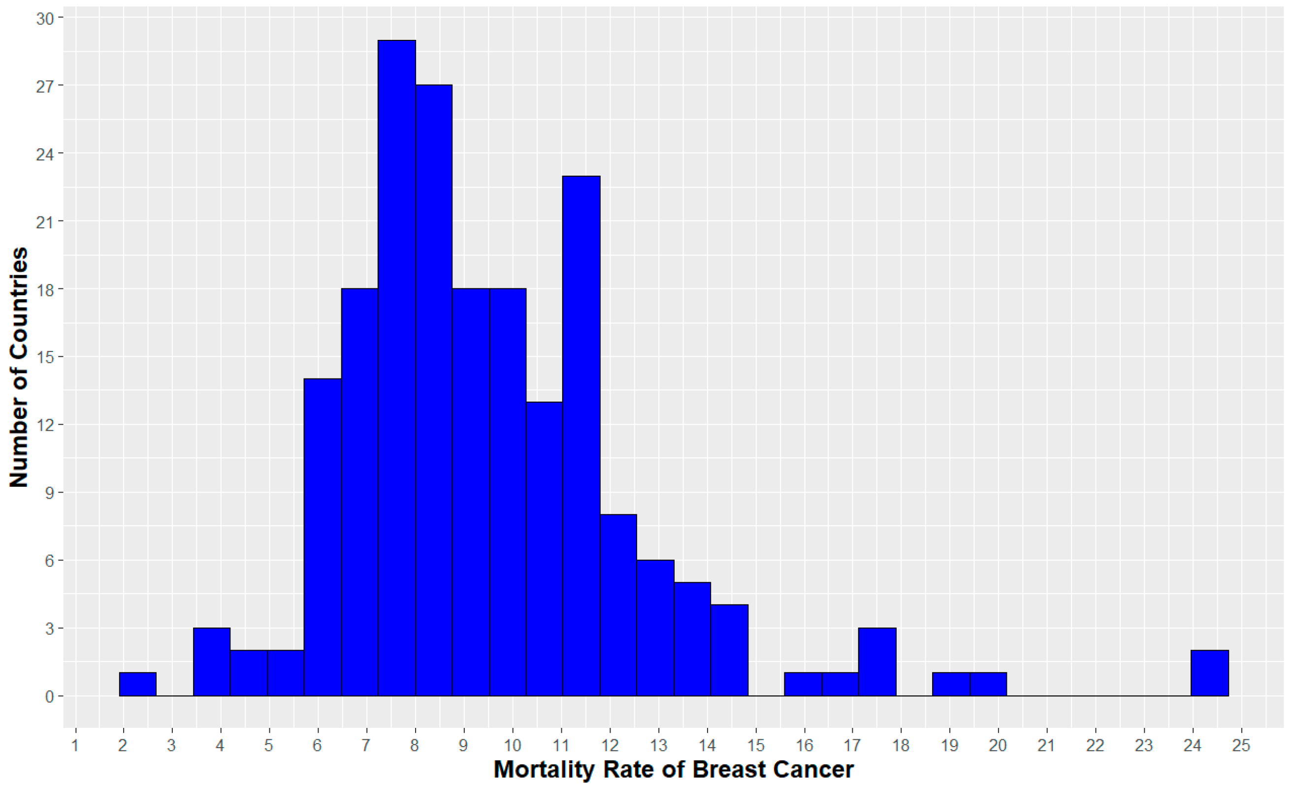
Figure 2.
Boxplots of the quantities belonging to the “benign” and “malignant” samples in the WBC dataset.
Figure 2.
Boxplots of the quantities belonging to the “benign” and “malignant” samples in the WBC dataset.
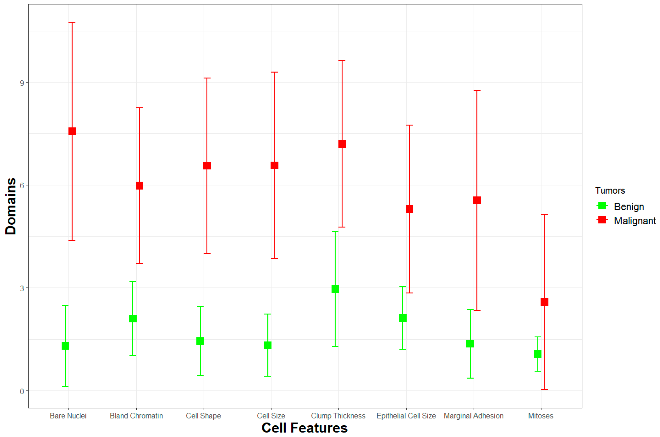
Figure 3.
Histograms of eight quantities taken values from 1-10 according to “benign” and “malignant” status in the WBC dataset.
Figure 3.
Histograms of eight quantities taken values from 1-10 according to “benign” and “malignant” status in the WBC dataset.
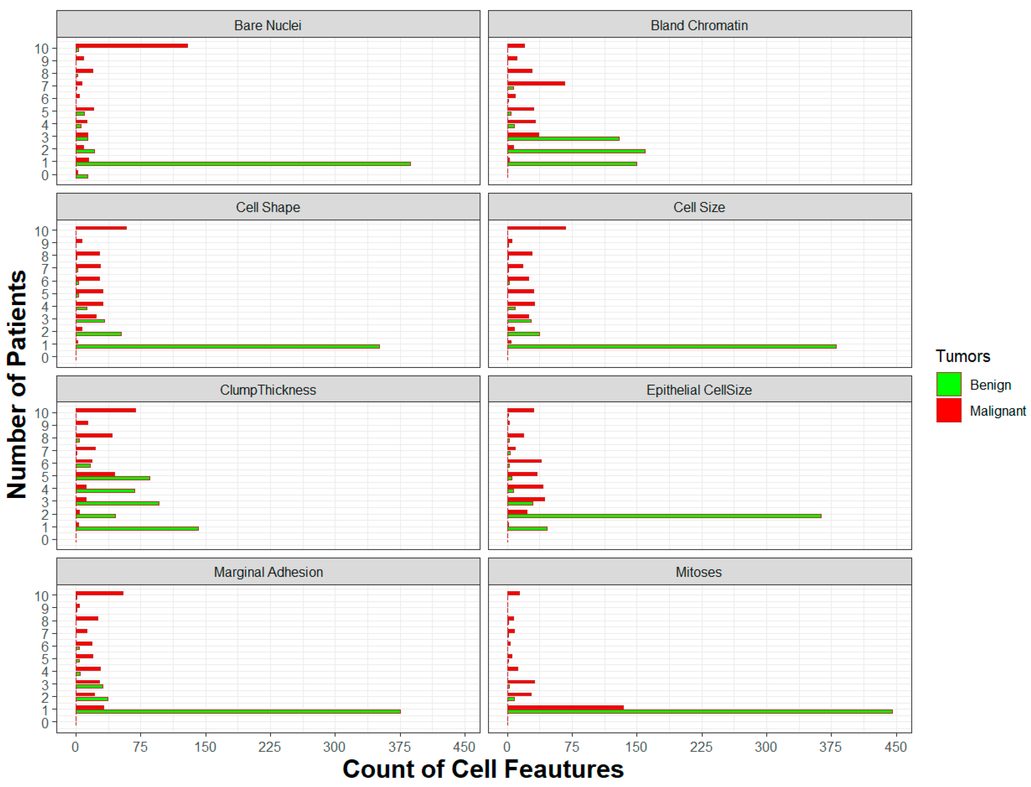
Table 1.
Descriptive statistics for 699 sample points according to their “benign” or “malignant” status of eight different quantities in the WBC dataset.
Table 1.
Descriptive statistics for 699 sample points according to their “benign” or “malignant” status of eight different quantities in the WBC dataset.
| Variables | Benign | Malignant | ||||||
|---|---|---|---|---|---|---|---|---|
| Min. | Median | Mean Sd. | Max. | Min. | Median | Mean Sd. | Max. | |
| Clump Thickness |
1 | 3 | 2.9563 1.6743 | 8 | 1 | 8 | 7.195 2.4288 | 10 |
| Cell Size | 1 | 1 | 1.3253 0.9077 | 9 | 1 | 6 | 6.5726 2.7195 | 10 |
| Cell Shape | 1 | 1 | 1.4432 0.9978 | 8 | 1 | 6 | 6.5602 2.562 | 10 |
| Marginal Adhesion |
1 | 1 | 1.3646 0.9968 | 10 | 1 | 5 | 5.5477 3.2105 | 10 |
| Epithelial Cell Size | 1 | 2 | 2.1201 0.9171 | 10 | 1 | 5 | 5.2988 2.4516 | 10 |
| Bare Nuclei | 0 | 1 | 1.3057 1.1827 | 10 | 0 | 10 | 7.5643 3.1802 | 10 |
| Bland Chromatin |
1 | 2 | 2.1004 1.0803 | 7 | 1 | 7 | 5.9793 2.2739 | 10 |
| Mitoses | 1 | 1 | 1.0633 0.5020 | 8 | 1 | 1 | 2.5892 2.5579 | 10 |
Table 2.
Descriptive statistics of totally 699 sample points according to their “benign” and “malignant” status, eight different groups, and eight different quantities in the WBC dataset.
Table 2.
Descriptive statistics of totally 699 sample points according to their “benign” and “malignant” status, eight different groups, and eight different quantities in the WBC dataset.
| Clump Thickness | Cell Size | Cell Shape | Marginal Adhesion | Epithelial Cell Size | Bare Nuclei | Bland Chromatin | Mitoses | ||||||||||
| Malign | Benign | Malign | Benign | Malign | Benign | Malign | Benign | Malign | Benign | Malign | Benign | Malign | Benign | Malign | Benign | ||
| Group 1 | Min. | 1 | 1 | 1 | 1 | 1 | 1 | 1 | 1 | 1 | 1 | 0 | 0 | 1 | 1 | 1 | 1 |
| Median | 2 | 8 | 1 | 6 | 1 | 6 | 1 | 4 | 2 | 5 | 1 | 10 | 3 | 5 | 1 | 1 | |
| Mean Sd. | 2.675 1.7333 | 7.3054 2.434 | 1.375 1.0439 | 6.1257 2.7685 | 1.475 1.1384 | 6.2575 2.5197 | 1.33, 0.9674 |
5.1796 3.2157 | 2.24 1.1658 |
5.4072 2.6255 | 1.43 1.5154 |
7.6168 3.1215 | 2.6 1.1988 |
5.3892 2.0648 | 1.08 0.5432 |
2.8204 2.6826 | |
| Max. | 8 | 10 | 8 | 10 | 8 | 10 | 9 | 10 | 10 | 10 | 10 | 10 | 7 | 10 | 7 | 10 | |
| Group 2 | Min. | 1 | 3 | 1 | 5 | 1 | 3 | 1 | 1 | 1 | 2 | 0 | 1 | 1 | 2 | 1 | 1 |
| Median | 3 | 9 | 1 | 8 | 1 | 8 | 1 | 5 | 2 | 5 | 1 | 10 | 2 | 7 | 1 | 1 | |
| Mean Sd. | 2.7544 1.5616 | 8.3077 2.213 | 1.6842 1.27 |
8.0769 1.801 | 1.7895 1.2209 | 8 2.1213 |
1.4737 1.0369 | 4.9231 3.0947 | 2.2105 0.7731 | 5.6923 2.9264 | 1.2807 1.0816 | 8.1538 3.3874 | 1.9298 0.7526 | 6.8462 2.035 | 1.0526 0.2941 | 1.9231 2.06 | |
| Max. | 6 | 10 | 9 | 10 | 7 | 10 | 6 | 10 | 5 | 10 | 8 | 10 | 4 | 10 | 3 | 8 | |
| Group 3 | Min. | 1 | 4 | 1 | 2 | 1 | 2 | 1 | 1 | 1 | 2 | 1 | 3 | 1 | 1 | 1 | 1 |
| Median | 4 | 10 | 1 | 6 | 1 | 6 | 1 | 7 | 2 | 5 | 1 | 10 | 1 | 8 | 1 | 1 | |
| Mean Sd. | 3.6364 1.6197 | 8.1111 2.4721 | 1.1364 0.4676 | 5.8889 2.0883 | 1.2727 0.6311 | 5.8889 2.4721 | 1.9091 1.377 | 6.1111 2.9768 | 2 0.4364 |
4.7778 1.3944 | 1.4545 1.101 | 8.1111 2.9345 | 1.0909 0.2942 | 7.7778 2.8186 | 1 0 |
1.4444 0.7265 | |
| Max. | 6 | 10 | 3 | 9 | 3 | 9 | 6 | 10 | 3 | 6 | 5 | 10 | 2 | 10 | 1 | 3 | |
| Group 4 | Min. | 1 | 4 | 1 | 7 | 1 | 7 | 1 | 5 | 1 | 4 | 1 | 5 | 1 | 7 | 1 | 1 |
| Median | 4.5 | 8 | 1 | 8 | 1 | 8 | 1 | 10 | 2 | 5 | 1 | 10 | 1 | 9 | 1 | 1 | |
| Mean Sd. | 4.2857 1.326 | 7 2.6458 |
1.2143 0.5789 | 8.3333 1.5275 | 1.2857 0.4688 | 8.3333 1.5275 | 1.3571 0.9288 | 8.3333 2.8868 | 1.7857 0.4258 | 6.3333 3.2146 | 1 0 |
8.3333 2.8868 | 1.1429 0.3631 | 8.6667 1.5275 | 1 0 |
4 5.1962 |
|
| Max. | 6 | 9 | 3 | 10 | 2 | 10 | 4 | 10 | 2 | 10 | 1 | 10 | 2 | 10 | 1 | 10 | |
| Group 5 | Min. | 1 | 3 | 1 | 3 | 1 | 2 | 1 | 1 | 1 | 3 | 1 | 3 | 1 | 3 | 1 | 1 |
| Median | 3.5 | 6 | 1 | 6.5 | 1 | 6.5 | 1 | 8.5 | 2 | 3.5 | 1 | 10 | 1.5 | 6.5 | 1 | 1 | |
| Mean Sd. | 3.1389 1.5703 | 6.25 2.2613 |
1.1111 0.3984 | 6.9167 2.6443 | 1.1389 0.4245 | 6.5833 2.811 | 1.4167 1.5376 | 6.8333 3.5633 | 1.8333 0.6547 | 4.0833 1.4434 | 1.25 0.8742 |
8.0833 2.8749 | 1.6111 0.6878 | 6.3333 2.0151 | 1 0 |
2 1.954 |
|
| Max. | 6 | 10 | 3 | 10 | 3 | 10 | 10 | 10 | 4 | 7 | 5 | 10 | 3 | 9 | 1 | 7 | |
| Group 6 | Min. | 1 | 5 | 1 | 4 | 1 | 3 | 1 | 1 | 1 | 3 | 1 | 2 | 1 | 2 | 1 | 1 |
| Median | 3.5 | 7 | 1 | 8 | 1 | 8 | 1 | 6 | 2 | 5 | 1 | 10 | 2 | 7 | 1 | 1 | |
| Mean Sd. | 3.425 1.534 | 7.3333 1.8708 | 1.225 0.6597 | 7.8889 2.0883 | 1.275 0.5541 | 7.3333 2.958 | 1.15 0.4267 |
6.2222 3.3082 | 1.925 0.2667 | 5 1.5 |
1.175 0.7121 | 8 3.1225 |
2.225 0.7675 | 7.4444 2.4037 | 1.025 0.1581 | 1.3333 0.5 |
|
| Max. | 6 | 10 | 4 | 10 | 3 | 10 | 3 | 10 | 2 | 8 | 5 | 10 | 4 | 10 | 2 | 2 | |
| Group 7 | Min. | 1 | 2 | 1 | 3 | 1 | 2 | 1 | 3 | 1 | 3 | 1 | 1 | 1 | 4 | 1 | 1 |
| Median | 4 | 5.5 | 1 | 8 | 1 | 7.5 | 1 | 8 | 2 | 4.5 | 1 | 10 | 1 | 7.5 | 1 | 1 | |
| Mean Sd. | 3.7647 1.5219 | 6.5 2.6239 |
1.0588 0.2425 | 7.1429 2.9576 | 1.4118 0.8703 | 7.0714 2.8138 | 1.3529 1.2217 | 7.2857 2.7012 | 1.9412 0.4287 | 4.9286 1.7744 | 1 0 |
7.5 3.8381 |
1.5294 0.6243 | 7.5714 2.0273 | 1 0 |
1.9286 2.4008 | |
| Max. | 5 | 10 | 2 | 10 | 4 | 10 | 6 | 10 | 3 | 10 | 1 | 10 | 3 | 10 | 1 | 10 | |
| Group 8 | Min. | 1 | 3 | 1 | 6 | 1 | 4 | 1 | 1 | 1 | 3 | 0 | 1 | 1 | 4 | 1 | 1 |
| Median | 3 | 5 | 1 | 10 | 1 | 8 | 1 | 6 | 2 | 5 | 1 | 5 | 1.5 | 7 | 1 | 2.5 | |
| Mean Sd. | 2.8889 1.5883 | 5.7143 2.1989 | 1.2083 0.5799 | 8.8571 1.4601 | 1.4167 0.9154 | 7.8571 2.2483 | 1.3056 0.6846 | 6.2857 2.8401 | 2.1111 0.7792 | 5.3571 1.9057 | 1.1667 0.7121 | 5.2143 3.2148 | 1.6528 0.8419 | 7.6429 2.0979 | 1.125 0.8381 | 2.8571 2.627 | |
| Max. | 7 | 10 | 4 | 10 | 5 | 10 | 3 | 10 | 8 | 10 | 5 | 10 | 6 | 10 | 8 | 10 | |
Table 3.
The frequencies and relative frequencies of eight quantities according to “benign”, “malignant”, and both status of these sample groups in the WBC dataset.
Table 3.
The frequencies and relative frequencies of eight quantities according to “benign”, “malignant”, and both status of these sample groups in the WBC dataset.
| Quantities | Domain | ||||||||||
| Type | 1 | 2 | 3 | 4 | 5 | 6 | 7 | 8 | 9 | 10 | |
| Clump Thickness | Benign | 142 (31 %) | 46 (10.04 %) | 96 (20,96 %) | 68 (14,85 %) | 85 (18,56 %) | 16 (3,49 %) | 1 (0,22 %) | 4 (0,87 %) | 0 (0 %) |
0 (0 %) |
| Malign | 3 (1,24 %) | 4 (1,66 %) | 12 (4,98 %) | 12 (4,98 %) | 45 (18,67 %) | 18 (7,47 %) | 22 (9,13 %) | 42 (17,43 %) | 14 (5,81 %) | 69 (28,63 %) | |
| Both | 145 (20,74 %) | 50 (7,15 %) | 108 (15,45 %) | 80 (11,44 %) | 130 (18,6 %) | 34 (4,86 %) | 23 (3,29 %) | 46 (6,58 %) | 14 (2 %) | 69 (9,87 %) | |
| Cell Size | Benign | 380 (82,97 %) | 37 (8,08 %) | 27 (5,9 %) | 9 (1,97 %) | 0 (0 %) |
2 (0,44 %) | 1 (0,22 %) | 1 (0,22 %) | 1 (0,22 %) | 0 (0 %) |
| Malign | 4 (1,66 %) | 8 (3,32 %) | 25 (10,37 %) | 31 (12,86 %) | 30 (12,45 %) | 25 (10,37 %) | 18 (7,47 %) | 28 (11,62 %) | 5 (2,07 %) | 67 (27,8 %) | |
| Both | 384 (54,94 %) | 45 (6,44 %) | 52 (7,44 %) | 40 (5,72 %) | 30 (4,29 %) | 27 (3,86 %) | 19 (2,72 %) | 29 (4,15 %) | 6 (0,86 %) | 67 (9,59 %) | |
| Cell Shape | Benign | 351 (76,64 %) | 52 (11,35 %) | 33 (7,21 %) | 13 (2,84 %) | 3 (0,66 %) | 3 (0,66 %) | 2 (0,44 %) | 1 (0,22 %) | 0 (0 %) |
0 (0 %) |
| Malign | 2 (0,83 %) | 7 (2,9 %) | 23 (9,54 %) | 31 (12,86 %) | 31 (12,86 %) | 27 (11,2 %) | 28 (11,62 %) | 27 (11,2 %) | 7 (2,9 %) | 58 (24,07 %) | |
| Both | 353 (50,5 %) | 59 (8,44 %) | 56 (8,01 %) | 44 (6,29 %) | 34 (4,86 %) | 30 (4,29 %) | 30 (4,29 %) | 28 (4,01 %) | 7 (1 %) |
58 (8,3 %) | |
| Marginal Adhesion | Benign | 375 (81,88 %) | 37 (8,08 %) | 31 (6,77 %) | 5 (1,09 %) | 4 (0,87 %) | 4 (0,87 %) | 0 (0 %) |
0 (0 %) |
1 (0,22 %) | 1 (0,22 %) |
| Malign | 32 (13,28 %) | 21 (8,71 %) | 27 (11,2 %) | 28 (11,62 %) | 19 (7,88 %) | 18 (7,47 %) | 13 (5,39 %) | 25 (10,37 %) | 4 (1,66 %) | 54 (22,41 %) | |
| Both | 407 (58,23 %) | 58 (8,3 %) | 58 (8,3 %) | 33 (4,72 %) | 23 (3,29 %) | 22 (3,15 %) | 13 (1,86 %) | 25 (3,58 %) | 5 (0,72 %) | 55 (7,87 %) | |
| Epithelial Cell Size | Benign | 46 (10,04 %) | 363 (79,26 %) | 29 (6,33 %) | 7 (1,53 %) | 5 (1,09 %) | 2 (0,44 %) | 3 (0,66 %) | 2 (0,44 %) | 0 (0 %) |
1 (0,22 %) |
| Malign | 1 (0,41 %) | 23 (9,54 %) | 43 (17,84 %) | 41 (17,01 %) | 34 (14,11 %) | 39 (16,18 %) | 9 (3,73 %) | 19 (7,88 %) | 2 (0,83 %) | 30 (12,45 %) | |
| Both | 47 (6,72 %) | 386 (55,22 %) | 72 (10,3 %) | 48 (6,87 %) | 39 (5,58 %) | 41 (5,87 %) |
12 (1,72 %) | 21 (3 %) |
2 (0,29 %) | 31 (4,43 %) | |
| Bare Nuclei | Benign | 387 (84,5 %) | 21 (4,59 %) | 14 (3,06 %) | 6 (1,31 %) | 10 (2,18 %) | 0 (0 %) |
1 (0,22 %) | 2 (0,44 %) | 0 (0 %) |
3 (0,66 %) |
| Malign | 15 (6,22 %) | 9 (3,73 %) | 14 (5,81 %) | 13 (5,39 %) | 20 (8,3 %) | 4 (1,66 %) | 7 (2,9 %) |
19 (7,88 %) | 9 (3,73 %) | 129 (53,53 %) | |
| Both | 402 (57,51 %) | 30 (4,29 %) | 28 (4,01 %) | 19 (2,72 %) | 30 (4,29 %) | 4 (0,57 %) | 8 (1,14 %) | 21 (3 %) |
9 (1,29 %) | 132 (18,88 %) | |
| Bland Chromatin | Benign | 150 (32,75 %) | 159 (34,72 %) | 129 (28,17 %) | 8 (1,75 %) | 4 (0,87 %) | 1 (0,22 %) | 7 (1,53 %) | 0 (0 %) |
0 (0 %) |
0 (0 %) |
| Malign | 2 (0,83 %) | 7 (2,9 %) | 36 (14,94 %) | 32 (13,28 %) | 30 (12,45 %) | 9 (3,73 %) | 66 (27,39 %) | 28 (11,62 %) | 11 (4,56 %) | 20 (8,3 %) | |
| Both | 152 (21,75 %) | 166 (23,75 %) | 165 (23,61 %) | 40 (5,72 %) | 34 (4,86 %) | 10 (1,43 %) | 73 (10,44 %) | 28 (4,01 %) | 11 (1,57 %) | 20 (2,86 %) | |
| Mitoses | Benign | 445 (97,16 %) | 8 (1,75 %) | 2 (0,44 %) | 0 (0 %) |
1 (0,22 %) | 0 (0 %) |
1 (0,22 %) | 1 (0,22 %) | 0 (0 %) |
0 (0 %) |
| Malign | 134 (55,6 %) | 27 (11,2 %) | 31 (12,86 %) | 12 (4,98 %) | 5 (2,07 %) | 3 (1,24 %) | 8 (3,32 %) | 7 (2,9 %) |
0 (0 %) |
14 (5,81 %) | |
| Both | 579 (82,83 %) | 35 (5,01 %) | 33 (4,72 %) | 12 (1,72 %) | 6 (0,86 %) | 3 (0,43 %) | 9 (1,29 %) | 8 (1,14 %) | 0 (0 %) |
14 (2 %) |
|
Table 4.
Tabular representation and description of the confusion matrix for the GLM and GLMM approaches used in this study.
Table 4.
Tabular representation and description of the confusion matrix for the GLM and GLMM approaches used in this study.
| Predicted | |||
| Total Population |
Positive | Negative | |
| Actual | Positive | True Posisite | False Negative |
| Negative | False Positive | True Negative | |
Table 5.
Some performance metrics to compare the GLM and GLMM approaches used in this study.
| Performance Metrics | Abbreviations | Formulas | References |
| Accuracy | ACC | Metz [84], BSI [85] |
|
| Sensitivity (Recall, True Positive Rate) | TPR | Yerushalmy [86], Lewis [87], Lewis [88] |
|
| Specificity (Selectivity, True Negative Rate) | TNR | Yerushalmy [86] | |
| Precision (Positive Predictive Value) | PPV | Lewis [87], Lewis [88] |
|
| F1 Score | F1 | Chinchor et al. [89] |
Table 6.
Results of the binary regression models in the GLM approach under the logit, probit, cloglog and cauchit binary link functions for the WBC dataset.
Table 6.
Results of the binary regression models in the GLM approach under the logit, probit, cloglog and cauchit binary link functions for the WBC dataset.
| Link Functions | Explanatory Variables | ||||||
|---|---|---|---|---|---|---|---|
| Lower | Upper | ||||||
| logit | Intercept | -9.7417 | 1.0620 | <2e-16 * | 0.0001 | 0.0000 | 0.0005 |
| Clump Thickness | 0.5374 | 0.1354 | 7.23e-05 * | 1.7116 | 1.3126 | 2.2320 | |
| Cell Size | 0.0669 | 0.1821 | 0.71327 | 1.0692 | 0.7483 | 1.5278 | |
| Cell Shape | 0.3681 | 0.2038 | 0.07092 | 1.4449 | 0.9691 | 2.1544 | |
| Marginal Adhesion | 0.2398 | 0.1145 | 0.03625 * | 1.2710 | 1.0155 | 1.5909 | |
| Epithelial Cell Size | 0.0897 | 0.1517 | 0.55464 | 1.0938 | 0.8124 | 1.4726 | |
| Bare Nuclei | 0.4222 | 0.0899 | 2.61E-06 | 1.5253 | 1.2790 | 1.8191 | |
| Bland Chromatin | 0.4490 | 0.1568 | 0.00418 * | 1.5668 | 1.1523 | 2.1303 | |
| Mitoses | 0.5416 | 0.3110 | 0.08157 | 1.7187 | 0.9344 | 3.1616 | |
| probit | Intercept | -5.1152 | 0.4863 | <2e-16* | 0.0060 | 0.0023 | 0.0156 |
| Clump Thickness | 0.2689 | 0.0659 | 4.51e-05* | 1.3085 | 1.1499 | 1.4890 | |
| Cell Size | 0.0297 | 0.0927 | 0.7491 | 1.0301 | 0.8589 | 1.2355 | |
| Cell Shape | 0.2215 | 0.1008 | 0.0280* | 1.2480 | 1.0242 | 1.5207 | |
| Marginal Adhesion | 0.1093 | 0.0592 | 0.0648 | 1.1155 | 0.9933 | 1.2528 | |
| Epithelial Cell Size | 0.0553 | 0.0773 | 0.4742 | 1.0569 | 0.9083 | 1.2297 | |
| Bare Nuclei | 0.2195 | 0.0430 | 3.26e-07* | 1.2454 | 1.1448 | 1.3549 | |
| Bland Chromatin | 0.2313 | 0.0771 | 0.0027* | 1.2602 | 1.0835 | 1.4658 | |
| Mitoses | 0.2592 | 0.1393 | 0.0628 | 1.2959 | 0.9863 | 1.7027 | |
| cloglog | Intercept | -6.99164 | 0.60571 | <2e-16* | 0.0009 | 0.0003 | 0.0030 |
| Clump Thickness | 0.31983 | 0.06462 | 7.44e-07* | 1.3769 | 1.2131 | 1.5628 | |
| Cell Size | -0.01662 | 0.08392 | 0.84298 | 0.9835 | 0.8343 | 1.1594 | |
| Cell Shape | 0.32819 | 0.09544 | 0.00058* | 1.3885 | 1.1516 | 1.6741 | |
| Marginal Adhesion | 0.07062 | 0.05742 | 0.21871 | 1.0732 | 0.9589 | 1.2010 | |
| Epithelial Cell Size | 0.14707 | 0.07803 | 0.05945 | 1.1584 | 0.9941 | 1.3499 | |
| Bare Nuclei | 0.23099 | 0.03901 | 3.21e-09* | 1.2598 | 1.1671 | 1.3600 | |
| Bland Chromatin | 0.27925 | 0.07608 | 0.00024* | 1.3221 | 1.1390 | 1.5347 | |
| Mitoses | 0.26686 | 0.1283 | 0.03753* | 1.3059 | 1.0155 | 1.6792 | |
| cauchit | Intercept | -34.0342 | 9.2132 | 0.00022* | 0.0000 | 0.0000 | 0.0000 |
| Clump Thickness | 1.6139 | 0.5607 | 0.00400* | 5.0224 | 1.6735 | 15.0725 | |
| Cell Size | 1.2674 | 0.6981 | 0.069441 | 3.5516 | 0.9040 | 13.9527 | |
| Cell Shape | 2.5983 | 0.9536 | 0.00644* | 13.4409 | 2.0735 | 87.1261 | |
| Marginal Adhesion | 0.5877 | 0.3087 | 0.056899 | 1.7998 | 0.9828 | 3.2961 | |
| Epithelial Cell Size | -0.4612 | 0.3948 | 0.242818 | 0.6305 | 0.2908 | 1.3670 | |
| Bare Nuclei | 2.2314 | 0.6716 | 0.00089* | 9.3129 | 2.4969 | 34.7346 | |
| Bland Chromatin | 0.8428 | 0.5632 | 0.13454 | 2.3229 | 0.7702 | 7.0053 | |
| Mitoses | 2.2195 | 1.1861 | 0.06131 | 9.2027 | 0.9001 | 94.0904 | |
Table 7.
Results of of the binary mixed regression models in the GLMM approach under the logit, probit, cloglog, and cauchit link functions with “group” random effect for the WBC dataset.
Table 7.
Results of of the binary mixed regression models in the GLMM approach under the logit, probit, cloglog, and cauchit link functions with “group” random effect for the WBC dataset.
| Link Functions | Explanatory Variables | 95% Confidence Level for | |||||
| Lower | Upper | ||||||
| logit | Intercept | -9.7417 | 1.0620 | <2e-16* | 0.0001 | 0.0000 | 0.0005 |
| Clump Thickness | 0.5374 | 0.1354 | 7.23e-05* | 1.7116 | 1.3126 | 2.2320 | |
| Cell Size | 0.0669 | 0.1821 | 0.71327 | 1.0692 | 0.7483 | 1.5278 | |
| Cell Shape | 0.3681 | 0.2038 | 0.0709 | 1.4449 | 0.9691 | 2.1544 | |
| Marginal Adhesion | 0.2398 | 0.1145 | 0.03625* | 1.2710 | 1.0155 | 1.5909 | |
| Epithelial Cell Size | 0.0897 | 0.1517 | 0.55464 | 1.0938 | 0.8124 | 1.4726 | |
| Bare Nuclei | 0.4222 | 0.0899 | 2.61e-06* | 1.5253 | 1.2790 | 1.8191 | |
| Bland Chromatin | 0.4490 | 0.1568 | 0.00418* | 1.5668 | 1.1523 | 2.1303 | |
| Mitoses | 0.5416 | 0.3110 | 0.08157 | 1.7187 | 0.9344 | 3.1616 | |
| probit | Intercept | -5.11523 | 0.48457 | <2e-16* | 0.0060 | 0.0023 | 0.0155 |
| Clump Thickness | 0.26891 | 0.06747 | 6.73e-05* | 1.3085 | 1.1464 | 1.4935 | |
| Cell Size | 0.02967 | 0.09444 | 0.75343 | 1.0301 | 0.8560 | 1.2396 | |
| Cell Shape | 0.22152 | 0.10487 | 0.03466* | 1.2480 | 1.0161 | 1.5328 | |
| Marginal Adhesion | 0.10932 | 0.0574 | 0.05682 | 1.1155 | 0.9968 | 1.2484 | |
| Epithelial Cell Size | 0.0553 | 0.07852 | 0.48124 | 1.0569 | 0.9061 | 1.2327 | |
| Bare Nuclei | 0.21947 | 0.04211 | 1.87e-07* | 1.2454 | 1.1468 | 1.3526 | |
| Bland Chromatin | 0.2313 | 0.07684 | 0.00261* | 1.2602 | 1.0840 | 1.4651 | |
| Mitoses | 0.25921 | 0.14433 | 0.0725 | 1.2959 | 0.9766 | 1.7196 | |
| cloglog | Intercept | -6.9915 | 0.5798 | <2e-16* | 0.0009 | 0.0003 | 0.0029 |
| Clump Thickness | 0.3198 | 0.0681 | 2.66e-06* | 1.3769 | 1.2048 | 1.5735 | |
| Cell Size | -0.0166 | 0.0894 | 0.85262 | 0.9835 | 0.8255 | 1.1719 | |
| Cell Shape | 0.3282 | 0.1087 | 0.00252* | 1.3885 | 1.1221 | 1.7180 | |
| Marginal Adhesion | 0.0706 | 0.0614 | 0.25013 | 1.0732 | 0.9515 | 1.2104 | |
| Epithelial Cell Size | 0.1471 | 0.0855 | 0.08532 | 1.1584 | 0.9797 | 1.3697 | |
| Bare Nuclei | 0.2310 | 0.0396 | 5.39e-09* | 1.2598 | 1.1658 | 1.3615 | |
| Bland Chromatin | 0.2792 | 0.0726 | 0.00012* | 1.3221 | 1.1467 | 1.5244 | |
| Mitoses | 0.2669 | 0.1434 | 0.0628 | 1.3058 | 0.9858 | 1.7297 | |
| cauchit | Intercept | -34.0344 | 9.7337 | 0.00047* | 0.0000 | 0.0000 | 0.0000 |
| Clump Thickness | 1.6140 | 0.5278 | 0.00223* | 5.0229 | 1.7852 | 14.1327 | |
| Cell Size | 1.2679 | 0.6157 | 0.03947* | 3.5534 | 1.0630 | 11.8778 | |
| Cell Shape | 2.5982 | 1.0076 | 0.00992* | 13.4395 | 1.8651 | 96.8435 | |
| Marginal Adhesion | 0.5877 | 0.3256 | 0.0711 | 1.7998 | 0.9508 | 3.4071 | |
| Epithelial Cell Size | -0.4612 | 0.4024 | 0.25178 | 0.6305 | 0.2865 | 1.3875 | |
| Bare Nuclei | 2.2315 | 0.6837 | 0.00110* | 9.3138 | 2.4387 | 35.5718 | |
| Bland Chromatin | 0.8427 | 0.5186 | 0.10421 | 2.3226 | 0.8405 | 6.4183 | |
| Mitoses | 2.2184 | 1.0522 | 0.03501* | 9.1926 | 1.1689 | 72.2919 | |
Table 8.
Results of the binary mixed regression models in the GLMM approach under the logit, probit, cloglog, and cauchit link functions with “id” random effect for the WBC dataset.
Table 8.
Results of the binary mixed regression models in the GLMM approach under the logit, probit, cloglog, and cauchit link functions with “id” random effect for the WBC dataset.
| Link Functions | Explanatory Variables | 95% Confidence Level for | |||||
| Lower | Upper | ||||||
| logit | Intercept | -35.7502 | 0.0012 | <2e-16* | 0.0000 | 0.0000 | 0.0000 |
| Clump Thickness | 2.0682 | 0.0012 | <2e-16* | 7.9104 | 7.8911 | 7.9296 | |
| Cell Size | 0.3343 | 0.0013 | <2e-16* | 1.3970 | 1.3934 | 1.4006 | |
| Cell Shape | 1.4162 | 0.0013 | <2e-16* | 4.1212 | 4.1107 | 4.1318 | |
| Marginal Adhesion | 0.7265 | 0.0012 | <2e-16* | 2.0679 | 2.0629 | 2.0729 | |
| Epithelial Cell Size | 0.6289 | 0.0013 | <2e-16* | 1.8755 | 1.8707 | 1.8803 | |
| Bare Nuclei | 1.6063 | 0.0013 | <2e-16* | 4.9842 | 4.9717 | 4.9967 | |
| Bland Chromatin | 1.7385 | 0.0013 | <2e-16* | 5.6888 | 5.6746 | 5.7031 | |
| Mitoses | 1.7342 | 0.0012 | <2e-16* | 5.6643 | 5.6506 | 5.6781 | |
| probit | Intercept | -9.5614 | 0.0019 | <2e-16* | 0.0001 | 0.0001 | 0.0001 |
| Clump Thickness | 0.5102 | 0.0019 | <2e-16* | 1.6657 | 1.6596 | 1.6718 | |
| Cell Size | 0.2569 | 0.0020 | <2e-16* | 1.2929 | 1.2879 | 1.2979 | |
| Cell Shape | 0.2526 | 0.0020 | <2e-16* | 1.2874 | 1.2824 | 1.2924 | |
| Marginal Adhesion | 0.1723 | 0.0019 | <2e-16* | 1.1880 | 1.1836 | 1.1924 | |
| Epithelial Cell Size | 0.1059 | 0.0020 | <2e-16* | 1.1117 | 1.1074 | 1.1161 | |
| Bare Nuclei | 0.4757 | 0.0019 | <2e-16* | 1.6092 | 1.6031 | 1.6153 | |
| Bland Chromatin | 0.4538 | 0.0019 | <2e-16* | 1.5743 | 1.5684 | 1.5803 | |
| Mitoses | 0.4191 | 0.0019 | <2e-16* | 1.5206 | 1.5150 | 1.5262 | |
| cloglog | Intercept | -13.7073 | 0.0017 | <2e-16* | 0.0000 | 0.0000 | 0.0000 |
| Clump Thickness | 0.5358 | 0.0016 | <2e-16* | 1.7088 | 1.7036 | 1.7141 | |
| Cell Size | 0.2359 | 0.0017 | <2e-16* | 1.2660 | 1.2618 | 1.2703 | |
| Cell Shape | 0.5402 | 0.0017 | <2e-16* | 1.7164 | 1.7107 | 1.7221 | |
| Marginal Adhesion | 0.1428 | 0.0016 | <2e-16* | 1.1535 | 1.1500 | 1.1571 | |
| Epithelial Cell Size | 0.3906 | 0.0017 | <2e-16* | 1.4778 | 1.4729 | 1.4827 | |
| Bare Nuclei | 0.5884 | 0.0016 | <2e-16* | 1.8011 | 1.7956 | 1.8067 | |
| Bland Chromatin | 0.6811 | 0.0016 | <2e-16* | 1.9761 | 1.9700 | 1.9822 | |
| Mitoses | 0.5726 | 0.0017 | <2e-16* | 1.7729 | 1.7669 | 1.7788 | |
| cauchit | Intercept | -41.3991 | 11.5252 | 0.00033* | 0.0000 | 0.0000 | 0.0000 |
| Clump Thickness | 2.9538 | 0.9066 | 0.00112* | 19.1787 | 3.2442 | 113.3790 | |
| Cell Size | 0.3683 | 0.8930 | 0.68004 | 1.4453 | 0.2511 | 8.3193 | |
| Cell Shape | -0.2457 | 0.8710 | 0.77789 | 0.7822 | 0.1419 | 4.3123 | |
| Marginal Adhesion | 1.9768 | 0.6551 | 0.00255* | 7.2196 | 1.9993 | 26.0703 | |
| Epithelial Cell Size | 0.4090 | 0.5235 | 0.434632 | 1.5053 | 0.5395 | 4.1999 | |
| Bare Nuclei | 2.3869 | 0.7747 | 0.00206* | 10.8797 | 2.3833 | 49.6656 | |
| Bland Chromatin | 1.9481 | 0.7656 | 0.01094* | 7.0153 | 1.5644 | 31.4587 | |
| Mitoses | 3.3792 | 1.0396 | 0.00115* | 29.3473 | 3.8251 | 225.1611 | |
Table 9.
Results of the binary mixed regression models in the GLMM approach under the logit, probit, cloglog and cauchit link functions with “id and group” random effect for the WBC dataset.
Table 9.
Results of the binary mixed regression models in the GLMM approach under the logit, probit, cloglog and cauchit link functions with “id and group” random effect for the WBC dataset.
| Link Functions | Explanatory Variables | 95% Confidence Level for | |||||
| Lower | Upper | ||||||
| logit | Intercept | -37.3782 | 0.0025 | <2e-16* | 0.0000 | 0.0000 | 0.0000 |
| Clump Thickness | 2.1253 | 0.0025 | <2e-16* | 8.3754 | 8.3338 | 8.4172 | |
| Cell Size | 0.3621 | 0.0027 | <2e-16* | 1.4364 | 1.4288 | 1.4440 | |
| Cell Shape | 1.5250 | 0.0026 | <2e-16* | 4.5951 | 4.5717 | 4.6186 | |
| Marginal Adhesion | 0.7773 | 0.0025 | <2e-16* | 2.1756 | 2.1649 | 2.1864 | |
| Epithelial Cell Size | 0.6156 | 0.0026 | <2e-16* | 1.8508 | 1.8414 | 1.8603 | |
| Bare Nuclei | 1.6801 | 0.0025 | <2e-16* | 5.3661 | 5.3395 | 5.3928 | |
| Bland Chromatin | 1.7540 | 0.0025 | <2e-16* | 5.7774 | 5.7488 | 5.8062 | |
| Mitoses | 2.1798 | 0.0025 | <2e-16* | 8.8443 | 8.8009 | 8.8879 | |
| probit | Intercept | -11.1554 | 0.0013 | <2e-16* | 0.0000 | 0.0000 | 0.0000 |
| Clump Thickness | 0.6323 | 0.0013 | <2e-16* | 1.8820 | 1.8772 | 1.8868 | |
| Cell Size | 0.2335 | 0.0014 | <2e-16* | 1.2630 | 1.2596 | 1.2664 | |
| Cell Shape | 0.3308 | 0.0014 | <2e-16* | 1.3921 | 1.3884 | 1.3959 | |
| Marginal Adhesion | 0.2271 | 0.0013 | <2e-16* | 1.2549 | 1.2517 | 1.2582 | |
| Epithelial Cell Size | 0.0988 | 0.0014 | <2e-16* | 1.1039 | 1.1009 | 1.1068 | |
| Bare Nuclei | 0.5542 | 0.0013 | <2e-16* | 1.7406 | 1.7360 | 1.7452 | |
| Bland Chromatin | 0.5370 | 0.0013 | <2e-16* | 1.7109 | 1.7064 | 1.7154 | |
| Mitoses | 0.5032 | 0.0013 | <2e-16* | 1.6540 | 1.6496 | 1.6583 | |
| cloglog | Intercept | -15.1586 | 0.0015 | <2e-16* | 0.0000 | 0.0000 | 0.0000 |
| Clump Thickness | 0.6358 | 0.0015 | <2e-16* | 1.8885 | 1.8830 | 1.8939 | |
| Cell Size | 0.1922 | 0.0016 | <2e-16* | 1.2119 | 1.2082 | 1.2156 | |
| Cell Shape | 0.6651 | 0.0016 | <2e-16* | 1.9446 | 1.9387 | 1.9505 | |
| Marginal Adhesion | 0.2313 | 0.0015 | <2e-16* | 1.2603 | 1.2567 | 1.2639 | |
| Epithelial Cell Size | 0.4966 | 0.0016 | <2e-16* | 1.6432 | 1.6382 | 1.6482 | |
| Bare Nuclei | 0.5542 | 0.0015 | <2e-16* | 1.7405 | 1.7355 | 1.7456 | |
| Bland Chromatin | 0.7217 | 0.0015 | <2e-16* | 2.0579 | 2.0520 | 2.0639 | |
| Mitoses | 0.6025 | 0.0015 | <2e-16* | 1.8267 | 1.8213 | 1.8322 | |
| cauchit | Intercept | -41.3991 | 11.5111 | 0.00032* | 0.0000 | 0.0000 | 0.0000 |
| Clump Thickness | 2.9538 | 0.9057 | 0.00111* | 19.1787 | 3.2499 | 113.1792 | |
| Cell Size | 0.3683 | 0.8930 | 0.68003 | 1.4453 | 0.2511 | 8.3193 | |
| Cell Shape | -0.2457 | 0.8709 | 0.77786 | 0.7822 | 0.1419 | 4.3114 | |
| Marginal Adhesion | 1.9768 | 0.6546 | 0.00253* | 7.2196 | 2.0013 | 26.0447 | |
| Epithelial Cell Size | 0.4090 | 0.5235 | 0.4346 | 1.5053 | 0.5395 | 4.1999 | |
| Bare Nuclei | 2.3869 | 0.7739 | 0.00204* | 10.8797 | 2.3870 | 49.5878 | |
| Bland Chromatin | 1.9481 | 0.7651 | 0.01089* | 7.0153 | 1.5660 | 31.4279 | |
| Mitoses | 3.3792 | 1.0384 | 0.00114* | 29.3473 | 3.8341 | 224.6321 | |
Table 11.
Confusion matrix and some performance metrics for all of the models in this study.
| GLM | GLMM (group-random effect) | |||||||||||||||
| Link Functions | logit | probit | cloglog | cauchit | logit | probit | cloglog | cauchit | ||||||||
| Conf. Matrix | 447 | 11 | 448 | 10 | 449 | 9 | 448 | 10 | 453 | 5 | 444 | 14 | 447 | 11 | 448 | 10 |
| 11 | 230 | 13 | 228 | 18 | 223 | 16 | 225 | 7 | 234 | 12 | 229 | 16 | 225 | 6 | 235 | |
| ACC (Accuracy) | 0.96853 | 0.96710 | 0.96137 | 0.96280 | 0.9828326 | 0.96280 | 0.96137 | 0.97711 | ||||||||
| TPR (Sensitivity, Recall) | 0.97598 | 0.97817 | 0.98035 | 0.97817 | 0.989083 | 0.96943 | 0.97598 | 0.97817 | ||||||||
| TNR (Specificity) | 0.95436 | 0.94606 | 0.92531 | 0.93361 | 0.9709544 | 0.95021 | 0.93361 | 0.97510 | ||||||||
| PPV (Precision) | 1.85477 | 1.85892 | 1.86307 | 1.85892 | 1.879668 | 1.84232 | 1.85477 | 1.85892 | ||||||||
| F1 Score | 0.97598 | 0.97497 | 0.97081 | 0.97180 | 0.9869281 | 0.97155 | 0.97068 | 0.98246 | ||||||||
| GLMM (id-random effect) | GLMM (id and group random effects) | |||||||||||||||
| Link Functions | logit | probit | cloglog | cauchit | logit | probit | cloglog | cauchit | ||||||||
| Conf. Matrix | 456 | 4 | 447 | 11 | 446 | 12 | 440 | 18 | 451 | 7 | 450 | 8 | 450 | 8 | 445 | 13 |
| 3 | 238 | 9 | 232 | 10 | 231 | 14 | 227 | 4 | 237 | 13 | 228 | 4 | 237 | 5 | 236 | |
| ACC (Accuracy) | 0.98999* | 0.97139 | 0.96853 | 0.95422 | 0.9842632 | 0.969957 | 0.982833 | 0.974249 | ||||||||
| TPR (Sensitivity, Recall) | 0.99127* | 0.97598 | 0.97380 | 0.96070 | 0.9847162 | 0.982533 | 0.982533 | 0.971616 | ||||||||
| TNR (Specificity) | 0.98755* | 0.96266 | 0.95851 | 0.94191 | 0.9834025 | 0.946058 | 0.983402 | 0.979253 | ||||||||
| PPV (Precision) | 1.88382* | 1.85477 | 1.85062 | 1.82573 | 1.871369 | 1.86722 | 1.86722 | 1.846473 | ||||||||
| F1 Score | 0.99235* | 0.97812 | 0.97593 | 0.96491 | 0.9879518 | 0.977199 | 0.986842 | 0.980176 | ||||||||
Disclaimer/Publisher’s Note: The statements, opinions and data contained in all publications are solely those of the individual author(s) and contributor(s) and not of MDPI and/or the editor(s). MDPI and/or the editor(s) disclaim responsibility for any injury to people or property resulting from any ideas, methods, instructions or products referred to in the content. |
© 2023 by the authors. Licensee MDPI, Basel, Switzerland. This article is an open access article distributed under the terms and conditions of the Creative Commons Attribution (CC BY) license (http://creativecommons.org/licenses/by/4.0/).
Copyright: This open access article is published under a Creative Commons CC BY 4.0 license, which permit the free download, distribution, and reuse, provided that the author and preprint are cited in any reuse.


