Submitted:
30 September 2023
Posted:
01 October 2023
Read the latest preprint version here
Abstract
By framing the problem of determining the state of Schrodinger’s cat as a problem of searching for Hidden Markov Model (HMM), this work shows that there is a high chance that Schrodinger’s cat is dead with a stationary probabilities P(Cat = Dead) = 1, and P(Cat = Alive) = 0.
Keywords:
network analysis
; Hidden Markov Models
1. Introduction
The thought experiment popularly known as ‘Schrödinger’s Cat’ [1] is a widely known paradox in quantum mechanics used to frame the question of when exactly quantum superposition ends [2]. For years, this thought experiment has been debated and has been considered as a paradox that has no definite answer – the cat is dead and alive at the same time [3,4]. The current work confronts this conclusion of the paradox.
This current work shows that the probability of the cat being alive is not equal to the probability of the cat being dead amid making inference based on equally random observable states. This is done by framing the problem as a search for the Hidden Markov Model (HMM) [5,6] of the states of the cat. The problem model is schematically shown in Figure 1. With HMM, the states of the cat are hidden and must be computed using observable states that are affected by the hidden states. In this problem model, the observable states are the emotions of Schrödinger who directly observes the cat and shows two emotions – sad or happy – at equal prior probabilities (50% each) from each hidden state. We are the observers of these emotional states of Schrödinger, and we want to use these observations to estimate probabilities of the unknown states of the cat. The hidden state – cat being dead or cat being alive – has the following prior probabilities: if the cat is alive then it has equal chances of being alive (50%) or dead (50%), and if the cat is dead then it will remain dead (100%).
To estimate the posterior probabilities of the HMM states, a sequence of observations must be collected and used as inputs into the training of the network leading to a convergence of the probabilities of the hidden states. This set of observations can be synthetically generated from a random process. Because there are just two observable states, the sample generation process is a Bernoulli (p=0.50) process.
2. Methodology
The workflow in this work was implemented using the Python programming language. The Python codes in Jupyter Notebook files used in this work are curated in the online GitHub repository of the work: https://github.com/dhanfort/HMM_Schrod_cat.git.
2.1 Mathematical Formulation
The prior probabilities based on Figure 1 constitute the initial probabilities of the transition matrix and emission matrix . Matrices and would then be trained on the observable states to determine their posterior. The starting state matrix probability is fixed at equal probabilities . Rigorous mathematical derivations and explanations of the forward algorithm and updating algorithm in the training of HMM to learn and from observable states can be found in these references: [6,7]. The stationary probabilities of the hidden states were also computed.
2.2 Model Traning and Inference
The Python module ‘hmmlearn’ [8] was used to train the HMM. Datasets of observable states consisted of 10, 100, 1000, and 10000 samples were generated from a Bernoulli(p=0.5) implemented using the ‘random’ function in Numpy module [9]. The observable states were coded as follows: 0 = Sad, and 1 = Happy. The hidden states were coded as follows: 0 = Dead, and 1 = Alive. The ‘hmmlearn.CategoricalHMM’ function was used to model the HMM.
After training the HMM, the model was then used to predict the hidden states. The input datasets to this prediction step were a new set of observable states also generated via a Bernoulli(p=0.5) with 100 datasets each containing 100 observations states.
3. Results and Discussion
3.1. Stationary Probabilities
When looking at the model (Figure 1) in a long-term network propagation, the stationary probabilities of the hidden states could be computed. With the ‘hmmlearn’, this was computed using the ‘get_stationary_distribution()’ function in the HMM model. The resulting stationary probabilities were P(Cat = Dead) = 1.0 and P(Cat = Alive) = 0. These probabilities indicate that Schrödinger’s cat may be dead all along.
3.2. Observation-based Model Training
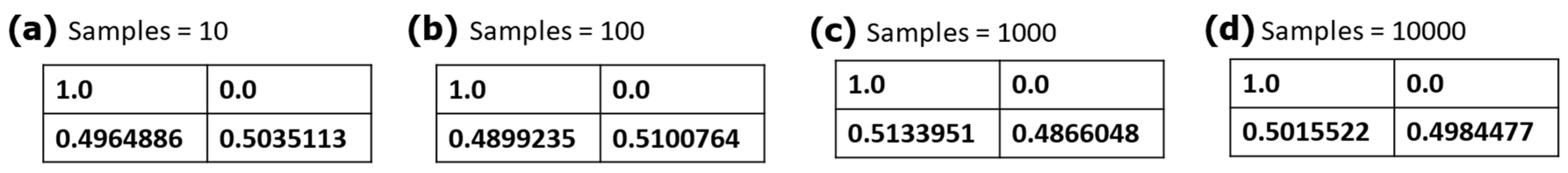
The stationary probabilities discussed in section 3.1 above were computed using the prior probabilities in the transition matrix (Figure 1). This begs the question “How good are the prior probabilities in the transition matrix used to compute the stationary probabilities of the hidden states?” We address this question by performing an observation-based learning through the fitting function in the ‘hmmlearn’ module, which fits the transition matrix . The transition matrix models the changes of hidden states in HMM and determining how observable states affect the transition probabilities would elucidate how the estimate of hidden state probabilities change. Based on our preliminary computations, the number of samples of the observable states significantly affect the updating of matrix . Figure 2 shows a graphical summary of tabulated results of the transition matrix at varying observable states sample. The resulting transition matrix values are close to the prior probabilities in the matrix . This indicates that the prior transition matrix used in the computation of the stationary probabilities is a good approximation of the hidden transition matrix. This confirms our conclusion that Schrödinger’s cat may be dead all along.
Author Contributions
Conceptualization, D.L.B.F. and A.P.M.; methodology, D.L.B.F.; software, D.L.B.F.; formal analysis, D.L.B.F. and A.P.M.; visualization, D.L.B.F. All authors have read and agreed to the published version of the manuscript.
Funding
This research received no external funding.
Data Availability Statement
The Python codes in Jupyter Notebook files used in this work are curated in the online GitHub repository of the work: https://github.com/dhanfort/HMM_Schrod_cat.git (accessed 29 September 2023).
Acknowledgments
We acknowledge the supportive staff of the Department of Chemical Engineering at the University of Louisiana at Lafayette, USA.
Conflicts of Interest
The authors declare no conflict of interest.
References
- Schrödinger, E. Die gegenwärtige Situation in der Quantenmechanik. Naturwissenschaften 1935, 23, 807–812. [Google Scholar] [CrossRef]
- Fine, A. The Einstein-Podolsky-Rosen Argument in Quantum Theory. The Stanford Encyclopedia of Philosophy 2020, Summer 2020. [Google Scholar]
- Trimmer, J.D. The Present Situation in Quantum Mechanics: A Translation of Schrödinger's "Cat Paradox" Paper. Proceedings of the American Philosophical Society 1980, 124, 323–338. [Google Scholar]
- Musser, G. Quantum paradox points to shaky foundations of reality. Available online: https://www.science.org/content/article/quantum-paradox-points-shaky-foundations-reality (accessed on 29 September 2023).
- Franzese, M.; Iuliano, A. Hidden Markov Models. In Encyclopedia of Bioinformatics and Computational Biology, Ranganathan, S., Gribskov, M., Nakai, K., Schönbach, C., Eds.; Academic Press: Oxford, 2019; pp. 753–762. [Google Scholar]
- Ghahramani, Z. An introduction to hidden Markov models and Bayesian networks. In Hidden Markov models: applications in computer vision; World Scientific Publishing Co., Inc., 2001; pp. 9–42. [Google Scholar]
- Rabiner, L.R. A tutorial on hidden Markov models and selected applications in speech recognition. Proceedings of the IEEE 1989, 77, 257–286. [Google Scholar] [CrossRef]
- hmmlearn-Developers. hmmlearn: Unsupervised learning and inference of Hidden Markov Models. Available online: https://hmmlearn.readthedocs.io/en/stable/ (accessed on 29 September 2023).
- Harris, C.R.; Millman, K.J.; van der Walt, S.J.; Gommers, R.; Virtanen, P.; Cournapeau, D.; Wieser, E.; Taylor, J.; Berg, S.; Smith, N.J.; et al. Array programming with NumPy. Nature 2020, 585, 357–362. [Google Scholar] [CrossRef]
Figure 1.
Formulation of the Schrödinger’s Cat paradox problem as a search for the Hidden Markov Model for the states of the cat. (a) Schrödinger sees whether the cat is dead or alive, but we can only observe Schrödinger’s emotions as we spy on Schrödinger. (b) Formulating the problem as a network model with the objective of determining the probabilities of the cat’s hidden states – Dead or Alive – by using Schrödinger’s observable states – Sad or Happy – as inputs to training the network model. The annotated probabilities are the prior probabilities.
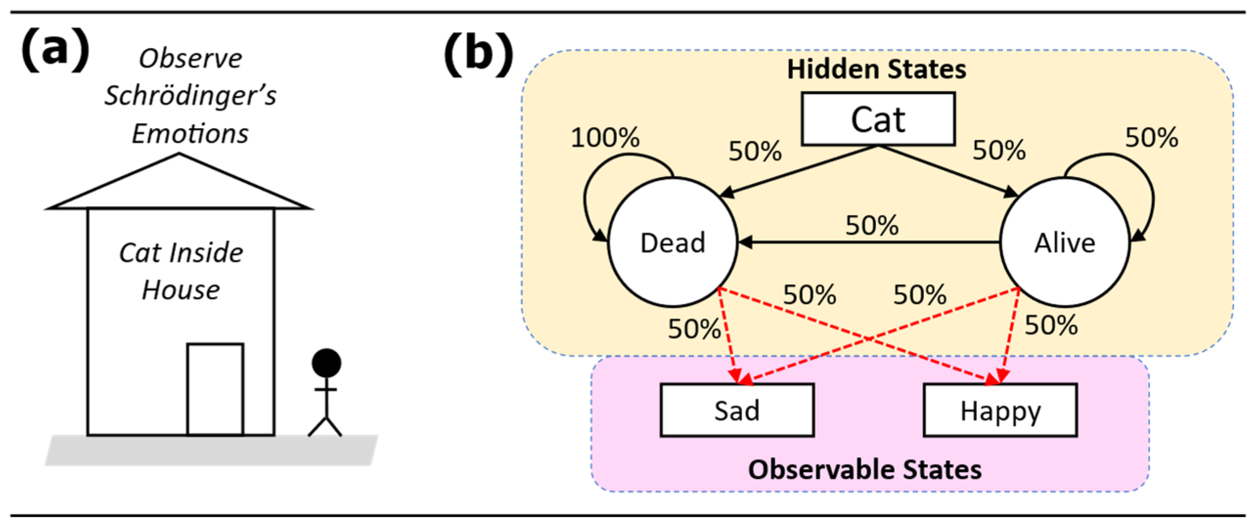
Figure 2.
The transition matrix after training on the the observable states at varying size of sample Bernoulli(p=0.5) samples: (a) 10 samples, (b) 100 samples, (c) 1000 samples, and (d) 10000 samples.
Figure 2.
The transition matrix after training on the the observable states at varying size of sample Bernoulli(p=0.5) samples: (a) 10 samples, (b) 100 samples, (c) 1000 samples, and (d) 10000 samples.
Disclaimer/Publisher’s Note: The statements, opinions and data contained in all publications are solely those of the individual author(s) and contributor(s) and not of MDPI and/or the editor(s). MDPI and/or the editor(s) disclaim responsibility for any injury to people or property resulting from any ideas, methods, instructions or products referred to in the content. |
© 2023 by the authors. Licensee MDPI, Basel, Switzerland. This article is an open access article distributed under the terms and conditions of the Creative Commons Attribution (CC BY) license (http://creativecommons.org/licenses/by/4.0/).
Copyright: This open access article is published under a Creative Commons CC BY 4.0 license, which permit the free download, distribution, and reuse, provided that the author and preprint are cited in any reuse.


