
Submitted:
16 September 2023
Posted:
18 September 2023
You are already at the latest version
Abstract
In this work, we incorporate a thixotropic-viscoelastic model into the widely used Computational Fluid Dynamics (CFD) software OpenFOAM, along with the rheoTool library. The model we implement is known as the Modified-Bautista-Manero (MBM), and effectively describes the rheological behavior of worm-like micellar solutions in extensional flows. We provide a detailed explanation of the numerical implementation of the model, specifically using the log-conformation tensor approach. Unlike previous works focused on this kind of fluids, we simulate inertial flows while considering convective terms in the governing equations, thus obtaining a more realistic behavior on the calculated results. The MBM model implementation is validated through numerical simulations on two different industrial-relevant geometries: the planar 4:1 contraction and the 4:1:4 contraction-expansion configurations. Furthermore, we investigate the influence of inertial, viscoelastic, and thixotropic effects on various flow field variables. These variables include velocity, viscosity, normal stresses, and corner vortex size. Our analysis encompasses both transient and steady solutions of corner vortexes across a range of Deborah and Reynolds numbers. Our results are also directly compared with simulations obtained using the non-thixotropic rubber network-based exponential Phan-Thien-Tanner (EPTT) model. From our planar 4:1 contraction results, we found that vortex-enhancement is seen when high elasticity is coupled with quick structural reformation and very low inertial effects. From our planar 4:1:4 contraction-expansion simulations, we show that an increase in inertia leads both to vortex-inhibition in the upstream channel and slight vortex-enhancement in the downstream channel. Lastly, we show the strong effect of the convection of fluidity into the fluidity profiles and into the upstream/downstream corner vortex sizes.
Keywords:
Computational Fluid Dynamics
; Finite Volume Method
; Rheology
; Non-Newtonian Fluids
; Viscoelasticity
; Thixotropy
; Worm-Like Micellar Solutions
1. Introduction
Viscoelastic fluids have been studied theoretically and experimentally for years, leading to the development of standard rheological models such as the Upper-Convected-Maxwell (UCM) [1], the quasi-linear elastic dumbbell Oldroyd-B [2], the non-linearly elastic Phan-Thien-Tanner (PTT) [3], the configuration-dependent molecular mobility Giesekus [4], among many others [5]. Also, the birth of Computational Fluid Dynamics (CFD) as a branch of science and the surge of computational power over the last decades has allowed researchers to simulate viscoelastic flow problems that were hard to tackle before [6], allowing in this way a better understanding of the models already developed and the formulation of new ones.
Some viscoelastic fluids show additional complex rheological behaviours. A common example of such fluids are the structured fluids, i.e., those materials that contain more than one phase, such as solid particles dispersed in a liquid, suspensions, surfactant solutions, among others, whose complex behaviour is generally dominated by the interactions between the components of the fluid. A typical example of a structured fluid is a micellar solution, which consists of a dispersion of micelles in a solvent. When surfactant molecules (which have a hydrophilic group (water-loving) that is chemically bonded to a hydrophobic group (water-hating)) are in the solution, they will self-assemble into aggregates such as spherical and wormlike micelles, bilayers, among others [7,8,9]. The rheological behaviour of micelles makes them highly attractive in the industry, specially in oil-recovery processes and in drilling operations [10,11,12,13]. Other examples of structured fluids include biological fluids [14] (such as blood [15]), colloidal and polymeric liquid systems, which also have direct application in the food, cosmetics, pharmaceutical and coating industries [16,17].
Entangled solutions of wormlike micelles exhibit viscoelastic effects, but they show special characteristics:
- At very low shear rates, their shear viscosity is constant (and slightly larger than that of the solvent), but more importantly, they are characterised by a single stress relaxation time (unlike some polymer solutions that exhibit a spectrum of relaxation times), yielding a near-Maxwell behaviour [18]. The response of these entangled solutions of wormlike surfactant solutions to unsteady shear-flows can be described with the standard Maxwell model.
- At higher shear rates, the entanglements may begin to break, so in order to model this kind of complex fluid, it is necessary to account for the reversible assembly and disassembly of the entangled wormlike-chain solution, which is usually modelled using a kinetic equation that could describe the level of internal structure of the fluid. Apart from viscoelasticity, these solutions can show thixotropy (defined as a time dependent property of structured fluids that exhibit a decrease in viscosity under flow, but there is a subsequent structural recovery once that the flow has been stopped) [19], yield-stress [20] and shear-banding [21,22].
It is of utmost importance to develop and study new constitutive equations that accurately capture the intricate behavior of these fluids. Therefore, in this work, our main focus is on the numerical implementation of the Modified-Bautista-Manero (MBM) viscoelastic model [23], and an in-depth analysis of the model’s behavior in contraction and expansion flows. The MBM model is particularly useful for accurately modeling the rheological behavior of micellar solutions, and, it encompasses essential characteristics like shear-thinning, shear-thickening, and thixotropic behaviors. The numerical implementation is performed using the widely-used and efficient open-source CFD software OpenFOAM, along with the rheoTool library [24]. This choice allows for a broader range of applications thanks to the software’s open-source nature. Furthermore, we provide a detailed explanation of the numerical implementation of the model, specifically using the log-conformation tensor approach, and we conduct an in-depth analysis of the model’s behavior when subject to strong extensional flows, such as the planar 4:1 contraction and 4:1:4 contraction-expansion geometries. These flows have only been previously documented in the literature for the inertialess case and in the absence of convective terms [25,26,27], and therefore, we improve our understanding of the model by performing simulations with a non-zero Reynolds number, which enables us to extend the model’s applicability. We are particularly interested in studying the transient and steady-state solutions of the corner vortex and how the coupled effects of viscoelasticity, thixotropy and inertia can affect their evolution. Three dimensionless numbers will be derived for a better analysis and understanding of our results. The content that will be presented here is an extension from our previous work [28], where simulations carried out in a recently developed software called HiGFlow [29], were compared with the results obtained in the rheoTool system. In the previous work [28], we limit ourselves to use fixed values of Deborah () and Reynolds () numbers in order to focus on the numerical validation of our solvers implemented in the HiGFlow software, which uses a new finite-difference method derived to simulate Newtonian and non-Newtonian flows in hierarchical grids [30].
Here, we delve deeper into understanding the behavior of thixotropic-viscoelastic fluids in contraction geometries, we explore a broader spectrum of Deborah and Reynolds numbers, and provide explanations for the observed phenomena through rheological reasoning. Our numerical findings are expected to serve as essential benchmarks for future experimental and theoretical simulations, contributing to the advancement of research in rheology and viscoelastic modeling.
The paper is organised as follows: Section 2 describes the thixotropic MBM model. Section 3 provides the complete system of governing equations and introduces a description of the discretization schemes and numerical methods employed in our simulations, which allow the stabilization of the viscoelastic fluid flow calculations. In Section 4, we present the numerical results obtained by the newly developed thixotropic viscoelastic model for two different flow geometries, the 4:1 contraction and the 4:1:4 contraction-expansion configurations. We provide detailed information on the technical aspects of our simulations, including the geometries, meshes, and other numerically relevant details. Furthermore, this section includes a discussion of how to interpret the obtained results, considering various Reynolds and Deborah numbers, as well as the structural relaxation parameter. Lastly, conclusions and future work are discussed in Section 5.
2. Thixotropic Models
In thixotropic systems, we observe that the immediate rheological properties, such as viscosity, are influenced by the internal structure level within the system. This level dynamically changes as the system undergoes deformation. The transformation of the internal microstructure of the fluid, and consequently, its viscosity, hinges on a delicate balance between two fundamental processes:
- Spontaneous Viscosity Build-Up (or Structural Reformation): This first process initiates when the structural parameter surpasses its minimum threshold, indicating a fully structured state. Importantly, the reformation is presumed to be independent of the rate at which shear work is exerted on the material. Instead, it relies on a material-specific characteristic time, which determines the pace of structural recovery for viscosity.
- Viscosity Breakdown (or Structural Destruction): In contrast to reformation, the breakdown of viscosity (second process) is directly influenced by the amount of shear work applied to the material. This process occurs when the structural parameter falls below its maximum value, signifying a completely unstructured state.
These two interdependent processes govern the dynamic behavior of thixotropic systems, where the viscosity response evolves in response to changing internal structures.
The BMP model [19] was first proposed in 1998 to predict and reproduce complex behaviour of viscoelastic systems that exhibit thixotropic and rheopectic characteristics. This model can accurately describe rheological flows of associative polymers, wormlike micellar solutions, dispersions of lamellar liquid crystals, and blood [15,19]. The model has five rheological parameters, which can be estimated from simple rheological experiments in steady and unsteady flows.
The simplest version of the BMP model consists of a coupled system of equations: a kinetic equation proposed by Fredrickson [31], which introduces a structural parameter to describe molecular entanglement, network junctions and destruction of structures (see Equation (1)), along with the Upper Convected Maxwell constitutive equation (see Equation (2)), which is assumed to model the complete wormlike micellar solution (the stress relaxation time is defined as , with the relaxation modulus, and, instead of the zero-shear-rate viscosity parameter, we now have ):
where t is the time, is the position vector, is the velocity field, is the extra-stress tensor, is the deformation-rate tensor,
and is the upper-convected derivative,
Equation (1) describes the evolution of the internal structure of the fluid , which is a structural parameter called fluidity, simply defined as the inverse of the viscosity ().
The right side of Equation (1) is divided in two terms:
- the first one is the reformation process (build up of viscosity or breakdown of fluidity), where is known as the structural relaxation time (units of ) and is the inverse of the zero-shear-rate viscosity, the fluidity plateau, and represents the fully structured state of the microstructure;
- the second term is the destruction process (breakdown of viscosity or build up of fluidity), where is a parameter related to structure breaking down (units of ), the term is the rate of energy dissipation of the fluid and is the experimentally observed fluidity at high shear rates, and represents the completely unstructured state of the fluid.
One of the disadvantages of this model is that the extensional viscosity gives rise to unbounded response (discontinuous structure) at finite deformation rates. In order to overcome the unbounded extensional viscosity response of the original model, Boek et al. [23], proposed a Modified-Bautista–Manero (MBM) model, where the constant solvent, , and polymeric, , viscosity contributions are split. Notice that, in the original model, see Equation (2), represents both the solvent and micellar parts.
The MBM model is then given by the total stress tensor that couples the solvent () and micellar/polymer () contributions to the solution:
together with the evolution equation for fluidity,
In this reformulation, the coefficient is treated as a single parameter and remains finite. Lastly, we should remark that in the original BMP model , where stands for the total zero shear-rate viscosity, i.e., , but in the MBM model . The MBM constitutive equation provides a continuous extensional viscosity response, which yields the possibility of supporting physically realistic strain-hardening/softening properties.
One of the novelties of this work compared to previous works found in the literature [25,26,27] is the inclusion of the convective term , which is included in the original thixotropic model derived by Fredrickson [31]. In the forthcoming results section, we will illustrate how convection of momentum, stress tensor, and fluidity play a significant role in contraction geometries. This is particularly pertinent when secondary flows manifest, making it evident that convective terms should not be entirely disregarded, as has been the case in previous papers.
A group of dimensionless numbers with physical relevant meaning can be derived from the MBM model. We scale fluidity with , lengths with L, we use the average shear rate (with being a characteristic velocity of the flow) to scale time and finally we scale stresses with a characteristic convective flux , leading to the dimensionless form of the kinetic equation for the fluidity:
where,
The dimensionless equations for the polymeric and solvent contributions are then given by (we kept again the original variables):
where we defined the solvent viscosity ratio as .
The Reynolds and Deborah numbers, are defined as follows,
with the fluid density, the zero-shear-rate viscosity obtained for the polymeric part and is the stress-relaxation time, defined as .
The parameter is associated to the reformation of complex structures and is commonly known as the dimensionless structural relaxation parameter, structure response rate or reformation parameter. The construction number represents the rate at which the material’s viscosity increases when subjected to a static or low shear stress. It quantifies the time required for the material to achieve a certain level of viscosity buildup after being at rest or subjected to low shear. For materials with high values of construction number (), the fluid will exhibit a slow or null relaxation of viscosity after the cessation of steady shear flow. On the other hand, fast structural relaxation is seen for the opposite case (). On the other hand, the parameter in Equation (10) is the parameter associated to the destruction/breaking down of structures. The destruction number represents the rate at which the material’s viscosity decreases when subjected to shear stress. It quantifies the time required for the material to recover its lower viscosity after being sheared or agitated. For a more in depth analysis of these dimensionless numbers the reader is refereed to inspect [25,32].
Boek et al. [23] compared directly the (shear and extensional) viscosities for a simple-steady shear flow and steady-state uniaxial extensional flow for both the BMP and the MBM models (see Figure 1 and 8 of their paper), and they showed that at intermediate values of strain rate, the extensional viscosity (dotted line) predicted by the original BMP model exhibits an odd behaviour, and therefore, the MBM model is recommended to use when simulating flows that involve extensional deformations. This is the main motivation that lead us to implement the MBM model in the rheoTool framework, and thus, we will carry out numerical simulations in these contraction-expansion geometries using only the MBM model.
3. Governing Equations and Numerical Method
The dimensionless equations governing the transient, isothermal and incompressible thixotropic-viscoelastic flows are the mass conservation and momentum equations (in the absence of external forces such as gravity):
together with,
where P is the dimensionless pressure.
3.1. Numerical method
As stated in Pimenta and Alves [33], numerical difficulties arise when solving the governing equations (14)–(18) at high Deborah numbers, which are mainly related from the insufficient resolution provided by discretization methods in capturing the rapid increase in stresses near critical points. In order to tackle this issue, Pimenta and Alves [33] implemented the log-conformation tensor approach proposed by Fattal and Kupferman [34] in the rheoTool computational framework, which consists in a reformulation of the differential constitutive equations in terms of the logarithm of the conformation tensor . The polymeric tensor is defined in terms of the conformation tensor as follows:
where is the identity tensor. In dimensionless form, this equation becomes:
For convenience, the viscoelastic equation with variable viscosity (17) is expressed in terms of the conformation tensor :
The log-conformation approach involves the introduction of a new tensor, denoted as , which is defined as the natural logarithm of the conformation tensor,
The conformation tensor can be diagonalized () since is positive definite, and is a matrix that contains in its columns the eigenvectors of and is a matrix whose diagonal elements are the eigenvalues resulting from the decomposition of . Thus, the new tensor can be written as follows:
Lastly, instead of solving the constitutive equation for the polymeric stress or for the conformation tensor, an evolution equation is derived for the natural logarithm of the conformation tensor (), which is obtained by reformulating equation (21) using the log-conformation approach:
In Equation (24), is an anti-symmetric tensor being the pure rotational component of the velocity gradient and is a symmetric tensor being the traceless extensional component of the velocity gradient. Details of this equation and the definitions of its terms are fully described in [24,33,35].
Then, the momentum equation is first solved to obtain an estimated velocity field, using previously known values of the pressure field. In the majority of CFD solvers, the continuity equation is formulated using the pressure variable, which is reduced to a Poisson-like differential equation. Once that this equation is solved, then the pressure field enforcing continuity is obtained, which is used to obtain a corrected velocity field. For a more detailed explanation of this approach, consult [24,33].
3.2. The exponential-PTT model
The Phan-Tien-Tanner (PTT) viscoelastic models [36] were derived from a Lodge-Yamamoto type of network theory for polymeric fluids. For this kind of models, network junctions are not assumed to move strictly as points of the continuum but allowed a certain “effective slip”. The rates of creation and destruction of junctions are assumed to depend on the instantaneous elastic energy of the network.
Several models have been derived from the original one, being one of the most popular in the scientific literature the exponential-Phan-Tien-Tanner (EPTT) [37], whose constitutive equation in terms of the conformation tensor is expressed as follows:
where is known as the extensibility parameter, which can determine the magnitude of the extensional viscosity. Equation (25) is the version of the model that considers affine motion, and the relation between polymer stress and conformation tensor is given by Equation (20).
The log-conformation version of Equation (25) is:
Tamaddon-Jahromi et al. [25] compared directly their inertialess simulations of planar-contraction 4:1 flows for the MBM model with the predictions of the EPTT model. They intended to illustrate the impact of the transient functionality of the worm-like micellar systems (with their assembly and disassembly properties) under complex deformation, where such transient description is absent in the EPTT network model. For these reasons, we will also carry out simulations under inertial conditions using the EPTT model. To do so, the momentum and continuity equations will be coupled with equations for the polymeric stress tensor (see Equation (20)) and the solvent contribution (see Equation (18)) along with the constitutive model (see Equation (25)), which will be transformed using the log-conformation approach previously described.
3.3. The RheoTool software
RheoTool [24] is an open-source toolbox based on OpenFOAM to simulate Generalized Newtonian Fluids (GNF) and viscoelastic fluids under pressure-driven and/or electrically-driven flows. The OpenFOAM/rheoTool framework uses a Finite Volume Method (FVM) approach for the numerical simulation of these flows. Full details and the theory behind the single-phase flow solvers used in rheoTool can be found in Pimenta and Alves [33] and Afonso et al. [35].
In the present work, we use the OpenFOAM version 7.0 together with rheoTool version 5.0. In all the simulations that will be carried out in rheoTool, we will use the solver rheoFoam, which implements the transient and incompressible Cauchy equation for single-phase flows of Generalized-Newtonian or viscoelastic fluids.
Some of the many features of rheoTool are: (1) a logarithm transformation of the conformation tensor () is implemented allowing to reach higher Deborah (or Weissenberg) numbers without loss of positive definiteness of the conformation tensor, (2) several techniques are available for stabilization purposes, for instance, the Rhie-Chow [38] interpolation allowing the coupling between pressure and velocity fields, and the both-sides-diffusion technique [39] allowing the coupling between stress and velocity fields, (3) high resolution schemes for the discretisation of advection terms following a component-wise deferred correction implementation, (4) constitutive equations library that contains a large amount of viscoelastic and GNF models, and (5) it includes interfaces to the sparse matrix solvers of external libraries, such as PETSc (Portable, Extensible Toolkit for Scientific Computation) [40], among other interesting features.
RheoTool allows the user to use the improved both-sides-diffusion (iBSD) technique [39], which consists in adding a diffusive term on both sides of the momentum Equation (15), with the difference that the one added in the left-hand side is added implicitly while the one in the right-hand side is added explicitly. Once steady state is reached, both terms cancel each other exactly. Such method increases the ellipticity of the momentum equation, and such, has a stabilizing effect on the numerical calculations. The iBSD technique will be used in all of our simulations to keep consistency with the results obtained in the previous work [28].
The following discretisation schemes were used: firstly, we used an Euler (transient, first order implicit and bounded) scheme for the time derivatives; secondly, all the advection terms were discretised using the CUBISTA (Convergent and Universally Bounded Interpolation Scheme for the Treatment of Advection) scheme [41]; a Gauss linear scheme was used for the gradient of the pressure and of the velocity, and for the divergence terms; lastly, the Laplacian terms were discretised using a Gauss linear corrected scheme. All the details of these schemes can be found in [42].
For the solution of the linear systems resulting from the discretization of the momentum equation (see Equation (15)) , the Bi-Conjugate Gradient Stabilized (Bi-CGSTAB) method [43] was used with a Simplified Diagonal-based Incomplete LU preconditioner (DILU), and for the pressure system (a Poisson equation obtained through the Rhie-Chow interpolation) the Conjugated Preconditioned Gradients (PCG) method was used with Simplified Diagonal-based Incomplete Cholesky (DIC) preconditioner [44].
3.4. Overview of the numerical method
Here, we briefly summarise the computational steps taken by the RheoTool software to simulate flows using the MBM fluid model:
- Initialise the fields for pressure p, velocity , fluidity (for the EPTT mode, ), log-conformation and polymeric stress tensors at time and set boundary conditions.
-
Enter the time loop ().
- (a)
-
Enter the inner iterations loop ().
- Compute the conformation tensor (Equation (19)) and their respective eigenvalues and eigenvectors and apply the log-conformation transformation approach to obtain the tensor .
- Solve the evolution of the log-conformation tensor Equation (24) to obtain .
- Solve the momentum equations for the velocity field that does not satisfy the continuity equation.
- Solve the Poisson equation for the pressure field and calculate the corrected velocity field ( and ).
- Increment the inner iteration index () and return to step i until the predefined number of inner iterations is reached.
- Update all the fields to be used in the next time loop: .
- (b)
- Increment the time and return to step 2 until the final time is reached.
- Stop the simulation and exit.
4. Results
In this study, we conduct simulations on fluids that display viscoelastic and thixotropic characteristics, examining two distinct configurations: the planar 4:1 contraction and the planar 4:1:4 contraction-expansion. To characterize this fluid behavior, we employ the MBM rheological model. Throughout the upcoming simulations, we will manipulate various model parameters, such as the structural relaxation parameter and Deborah number, in order to investigate different rheological behaviors. Additionally, we will explore the impact of inertia by varying the Reynolds number, specifically at values of . These findings will be elaborated upon in the subsequent sections.
4.1. The planar 4:1 contraction flow
In this section, we focus on describing the planar 4:1 contraction flow (see Figure 1), which offers a mix of shear and extensional deformation near the contraction region and where secondary flows might exist. This flow is a suitable benchmark problem for the evaluation of new rheological models or numerical methods [45].
Figure 1.
Domain representation: the planar 4:1 contraction geometry. Units are in meters.
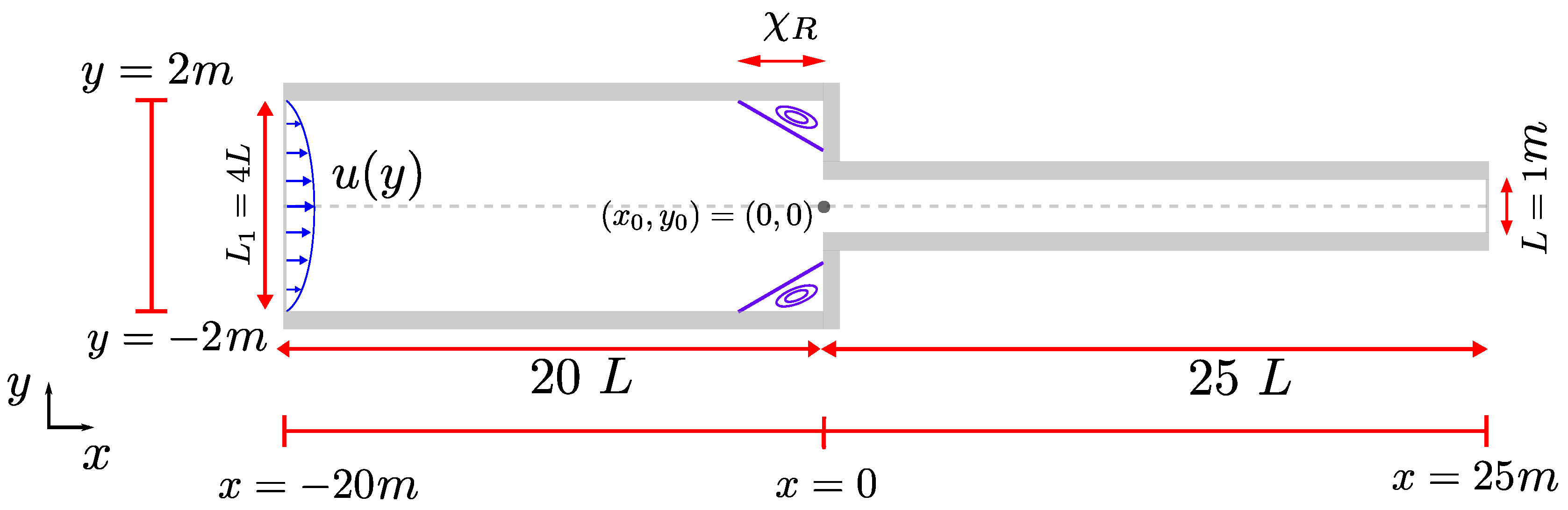
Some of the main characteristics of this geometry are: the characteristic length is defined as the width of the downstream channel m, and the width of the upstream channel is . In addition, we consider a large length for the upstream and downstream channels, respectively, and , to avoid artificial impact from the inlet and outlet boundaries on the obtained results. From our sketch of the domain, we can see that the origin (see Figure 1) is located where the contraction begins, exactly at the centreline of the downstream channel.
At the walls of the upstream and downstream channels, we impose the no-slip condition for the velocity and a linear extrapolation condition for the polymeric stress tensor. At the outlet, we set fully-developed boundary conditions and at the inlet, we adopt a parabolic profile of the form , where is the centreline velocity of the downstream channel.
Figure 2 illustrates the refined mesh, RMI, used on the numerical calculations of the 4:1 planar contraction configuration. As it can be seen, only half of the computational domain was used on the simulations since the flow is symmetric. This mesh has three levels of refinement (, and ), with the most refined region () near the contraction, inlet and outlet locations presenting cell sizes . The second level of refinement () has cell sizes and the third one () with cell sizes of .
We will also use three uniform meshes and an additional mesh with three refinement levels in order to check the convergence of the solutions. The uniform meshes are: mesh MI with , mesh MII with and mesh MIII with . The cell sizes of the second refined mesh RMII are half the value of the cell sizes of RMI for all refinement levels. The mesh convergence analysis is described in Section 4.1.1.
Finally, in all the simulations of the planar 4:1 sudden contraction problem, we will use the same time-step value and one inner iteration in the loop that solves the governing equations (see Section 3.4).
4.1.1. Mesh convergence analysis
In this section, we will carry out numerical simulations of the planar 4:1 contraction flow problem using the MBM model, with the main objective to perform a mesh convergence analysis to determine an optimal mesh refinement level that ensures results independent of the mesh resolution. The meshes that will be used on our analysis are those that were described in Section 4.1, i.e., the three uniform meshes MI, MII and MIII and two refined meshes RMI and RMII.
In order to perform the mesh convergence analysis, we will calculate the errors using the , and norms. We obtained the velocity profile on the downstream channel near the contraction region (at ) for each mesh, and we take the mesh MIII as reference mesh. Thus, the errors measuring the accuracy of the obtained results can be calculated using the following equations:
where is the solution in the mesh of reference MIII, is the solution of the respective mesh for which the error is being calculated (MI, MII, RMI and RMII), is the velocity profile in the points , where is a fixed point in the channel () and , .
For our simulations, we fixed the following parameter values: solvent viscosity ratio is , the Deborah number value is , the structural relaxation parameter is , the destruction parameter is and Reynolds number is . These values are standard parameter values used to model the behaviour of a viscoelastic flow with inertia that exhibits a quick structural recovery (low ). The results of the mesh convergence analysis are presented in Table 1, and it can be observed that while the solutions for all meshes are close to the solution obtained with mesh MIII, the refined meshes (particularly RMII, which has cell sizes near the contraction region equal to those of mesh MIII) show the smallest errors in terms of , , and . This suggests that it is not necessary to simulate thixotropic-viscoelastic flows using completely uniform meshes with extremely small cell sizes. In addition, apart from the fact that the solutions from refined meshes give us accurate values, they also help to reduce simulation time.
Now we compute the axial profiles of the velocity, viscosity and normal stresses at for each one of the meshes described above. The results can be seen in Figure 3 and Figure 4. As expected, it can be observed that the simulations in each of the five meshes (MI, MII, MIII, RMI and RMII) predicted a similar behaviour. However, we can easily see that the uniform mesh MI, which has the biggest cell sizes, tend to deviate from the numerical solutions of the rest of the meshes at . In addition, we see that decreasing the cell sizes the numerical results predicted using those meshes tend to be closer and closer to each other. Furthermore, the curve of the solutions obtained with meshes MII and RMI are in remarkable agreement (the same is observed for uniform mesh MIII and refined mesh RMII), and this is because the cell size value of the most refined level of mesh RMI has the same value as the value of the cells that composed the uniform mesh MII. These results prove that it is possible to obtain accurate results using locally refined meshes without the need to simulate flows with uniform meshes that have very small cell size values.
4.1.2. Strong-hardening and moderate-hardening behaviour
In this section, we will show results of our transient and steady-state simulations of the planar 4:1 contraction flow problem for the MBM model using the uniform and refined meshes described in Section 4.1. As previously mentioned, in all of our numerical results, we will use the log-conformation approach to solve the viscoelastic constitutive equation (see Equation (24)).
Following Tamaddon-Jahromi et al. [25], we will simulate two different cases: a fluid that exhibits strong-hardening and one with moderate-hardening. Some of the general fluid parameters that will be used in our simulations are shown in Table 2, where we take the centreline velocity and the width L of the downstream channel as the characteristic velocity and length, respectively, to calculate our dimensionless groups. We decide to calculate the Reynolds and Deborah numbers using L instead of the half-width because in our previous paper, we compare our results obtained here with numerical solutions of the MBM model from a new brand software called HiGFlow that uses the whole domain to carry out the simulations [28]. Different values of Deborah and Reynolds numbers (and thus, different values of and ) will be used for each fluid case in order to compare the effects of elasticity and inertia on the flow.
The model parameter values shown in Table 2 were selected by Tamaddon-Jahromi et al. [25] in order to match peaks in extensional viscosity () corresponding to instances of strong and moderate hardening. The viscosities predicted by the MBM model for cases 1 and 2 are comparable with the behaviour exhibited by a shear-thinning (non-thixotropic) exponential Phan-Thien/Tanner (EPTT) fluid (see Equation (25)), with an extensibility parameter value of to reproduce the strong-strain hardening case and to observe a moderate-hardening behaviour. In our previous work, we illustrated the planar extensional and shear () viscosities predicted by the MBM and EPTT models for both the moderate- and strong-hardening cases (see [28]).
As mentioned earlier, the most remarkable difference between our results and the ones reported in Tamaddon Jahromi et al. [25] is that we do not neglect inertial forces and convective terms are not ignored. The meshes to be used were already described in Section 4.1.
We start by showing the steady-state centreline axial velocity profiles near the contraction region ( and ) of the MBM fluids with strong- () and moderate- () hardening behaviour (see Figure 5). In addition, we show also the viscosity and normal stresses profiles of the MBM fluids with strong- () and moderate- () hardening behaviour (see Figure 6 and Figure 7, respectively). For each of these cases, we fixed the Deborah number and used three different values of Reynolds numbers, and . The simulations with correspond to the "creeping flow" case, where the inertial terms are almost negligible. As we already stated, most of previous works that focused on studying this geometry for this kind of fluids under creeping flow conditions ignored the left-hand side (both transient and convective terms) of the Cauchy equation (see Equation (15)) to simplify the solution of the system of equations. However, the contraction geometries can lead to the formation of secondary flows, which are important in the calculation of all the convective terms present in the momentum, fluidity and viscoelastic equations, and thus, such terms cannot be fully ignored. The software OpenFOAM/rheoTool easily let the users consider and discretise those terms using the CUBISTA method [41]. In this way, the creeping flow assumption is still adequate, notwithstanding the finite value of Reynolds number (). In all of our simulations, we will use the improved both-sides-diffusion technique (see Section 3.1).
In Figure 5, we show the dimensionless centreline axial velocity for the two cases, where we can see that we obtain the typical velocity profile for this kind of flows: the increasing extension rate causes the velocity to grow as we approach the contraction region ( and ) where we observe an overshoot behaviour (local maximum followed by a slow decrease). After this, the velocity reaches its steady-state value. We can also notice that, as expected, the velocity profiles are identical for the three different Reynolds number values.
The dimensionless profile of viscosity and the profiles of the normal stresses for a fluid with strong-hardening properties () can be found in Figure 6, where we take into account the influence of inertial and convective terms on their behavior. We illustrate the profile for the dimensionless viscosity (defined as the ratio between the viscosity and the zero-shear-rate viscosity) in Figure 6. As mentioned in previous sections, the viscosity is associated with the internal structure of our fluid. In this curve, we observe a similar pattern compared to the velocity profile: before the contraction region (), the fluid exhibits the same constant viscosity value , which means that the internal structure of the fluid has not changed (i.e. the complex micellar entanglement networks have not been destructed). However, as the fluid enters the contraction region, these networks are being broken due to flow, which causes a decrease in viscosity until it reaches a minimum value. More interestingly, since the fluid has thixotropic properties, the internal structure of the fluid is able to reform itself and thus, recovering its initial structure () as it moves away from the contraction region (). This quick structural recovery is also due to the magnitude of the value of the structural recovery parameter . Moreover, we can see that the flow with the higher Reynolds number (dotted line) exhibits the lowest minimum viscosity value at the centreline. For the other two Reynolds number cases, (solid red line) and (dashed line), the curves seem to be identical. However, small differences can be visualized if we zoom in the region near the centreline (see Figure 6), where we can see that the curve with is slightly lower compared to the creeping-flow case.
Now we study the normal stresses profiles and , which are shown in Figure 6 and Figure 6, respectively. The general behaviour of these curves is also the one we expected to see: overall, inertia will suppress the non-Newtonian (viscoelastic) effects. For the vs x curve, the values are zero very far away from the contraction region ( and ), but it reaches a maximum value at . The same behaviour is seen for but we see a minimum instead. In these profiles is where we can see the huge effects of the inertial terms on the normal stresses: for the profile, we can observe that the magnitude of the values of the curve with (red solid line) is way greater compared to the other two cases. Subsequently, the curve with is above the curve with the largest inertial effects () (see Figure 6). This behaviour was also expected since it is well known that the stresses are directly proportional to the Deborah number but inversely proportional to the Reynolds number. For the profiles, we have a similar scenario to that of the profiles for , but the values of are negative and we have a minimum instead (see Figure 6).
On the other hand, we have the dimensionless viscosity and the dimensional normal stresses profiles for the moderate-hardening case (), which are shown in Figure 7. All these profiles are similar to the ones already described for the strong-hardening case (see Figure 6). The main difference between the two thixotropic cases is the viscosity profile in Figure 7, where it can be noticed that the internal structure of the fluid is also being destructed as the fluid enters the contraction region, which causes a decrease on the viscosity. Since the structural destruction is high (or the structural recovery is weak), the fluid tends to reach a minimum value of , which is a smaller value compared to the value seen in the strong-hardening case (see Figure 6). Another interesting observation is that although the fluid also tries to recover its initial structure as the fluid moves away from the contraction region (), the structural recovery is not as quick compared to the strong-hardening case, and this is because of the fixed value that was setup for the construction number imposed in our simulations. This value of indicates the structural recovery is going to be slow [32].
As discussed in [28], something that caught our attention is that we can see that viscosity thins in the centreline, which is a region where extensional deformation prevails and the shear rates and the shear stress are null. However, the normal stresses and will have a contribution in the structural evolution of the fluid, since the dissipation term located on the right-hand side of the kinetic equation (see Equation (16)) will become at , where all terms are non-zero ( has a positive maximum value and has a negative minimum, see Figure 7 and Figure 7). More importantly, we can notice that for the simulations with inertia (), the Reynolds number appears on the term of Equation (16), indicating us that inertia will contribute to the structural destruction of the micellar solutions, leading to high values of fluidity (or low viscosity), which is in agreement with our results.
In addition, Tamaddon-Jahromi et al. [25] reported the transient development of the viscosity of a MBM fluid in planar 4:1 contraction inertialess flow using exactly the same MBM parameter values than us, and they observed that viscosity bands (with low viscosity values as a result of the shear-thinning nature of the fluid) spread out from the corner ( and ) to the centreline near the contraction region (see Figure 15 and 18 of their paper [25]). In Figure 8, we show the fluidity profiles at different times for our moderate-hardening simulation with and , where we can see that our results are in agreement with their observations: at small times , we notice that the fluidity is starting to increase (which is equivalent to a decrease in viscosity) near the corner. At higher times () and in steady-state, it is evident that the bands of fluidity have spread out from the corner and have reached the centreline of the geometry and even further away from the contraction (see the steady-state solution, Figure 8). The fluidity profiles observed for the strong-hardening case are shown in Figure 9, where it can be seen that the fluidity also increases (or equivalently, the viscosity decreases) at the centreline. It can also be noticed that viscosity bands spread out from the corner of the contraction. However, unlike the moderate-hardening case, these bands remain near the contraction region, as shown in the steady-state solution (see Figure 9).
4.1.3. Corner vortex: transient and steady-state behaviour
Our goal in this section is to study the transient and steady-state behaviour of the horizontal corner vortex size, (see Figure 1).
The strong- () and moderate- () hardening cases are studied here, which were simulated using the refined mesh RMI with exactly the same parameter values shown in Table 2. Simulations of the EPTT network model for strong- () and moderate- () hardening cases will also be carried out and will serve as a comparison point. Our methodology used for the calculation of the vortex size in the planar-contraction 4:1 geometry can be found in the appendix of our previous work [28]. Figure 10 shows the evolution of the steady-state dimensionless horizontal corner vortex size (scaled with the width of the downstream channel L) as a function of the Deborah number. For each value of and , we obtain the curves of vs for three different values of Reynolds number: , and . We will start by comparing our creeping-flow simulations with results already available in the literature to validate our solver. We focus first on the strong-hardening cases (figures to the left in Figure 10), where overall, we can see that there is a general pattern for the curves: a decrease of the vortex size is observed at small Deborah numbers but it is followed by a rapid increase at . This particular behaviour observed here is in agreement with reference works found in the literature, e.g., Pimenta et al. [33] saw similar patterns for the Oldroyd-B model while Tamaddon-Jahromi et al. [25] observed the same behavior in the MBM model for the inertialess case. In addition, Tamaddon-Jahromi et al. also noticed that there is a delayed departure in vortex behaviour from reduction-to-enhancement observed in the MBM results, which could be caused due to the slow strain-softening behaviour of the extensional viscosity of the EPTT model. Our simulations also predict similar results: for instance, from our creeping-flow simulations, we observe that the vortex size of the MBM model with fixed slightly decreases from to , and the vortex-enhancement is seen when . On the other hand, for the strong-hardening case of the EPTT model (), the decrease in is only seen from to , and the vortex size begins to increase at . Similar behaviour is also seen for the respective strong-hardening cases of each model. All the steady-state values of obtained for both the MBM and EPTT models in different flow conditions can be found in Table 3 and Table 4, whose content will be discussed later.
On the other hand, we have the moderate-hardening cases (figures to the right in Figure 10), and our creeping-flow () simulations also seem to be in agreement with what is being reported in [25]: Tamaddon-Jahromi et al. found that there is a significant vortex size reduction in the range for the EPTT model in comparison with the MBM solutions (see Figure 8 of their paper), which they attributed to the more rapid strain-softening behaviour of the MBM model. In our results, we can see that for the EPTT inertialess simulations (red lines), the vortex enhancement is seen at low Deborah numbers but a subsequent decrease of is seen at . In contrast, for the MBM results, although the vortex size remains almost constant at low , it begins to increase at and we manage to obtain stable simulations up to (with ), which corresponds to the critical Deborah number at and . It was expected to see vortex inhibition at , similar to the moderate-hardening case of the EPTT model, but numerical oscillations are present and stability cannot be guaranteed due to the inclusion of all the convective terms in the governing equations.
From these early results, Tamaddon-Jahromi et al. [25] also reported that the vortex tends to be greater in size for the moderate-hardening case in both models at low , while larger vortexes are seen at higher Deborah numbers for the strong-hardening behaviour predicted by the EPTT and MBM models, and once again, our simulations predict similar results: for instance, with both and fixed, a value of is seen with , while a value of is obtained with ; at higher Deborah numbers (), a value of is obtained for the strong-hardening case while is obtained for the moderate-hardening behaviour.
Now focusing on the inertial simulations (blue lines for the case while black lines are for ), we can notice that some of the observations previously made for the case still remain: 1) vortex decrease for the EPTT model and vortex-enhancement seen for the MBM results at moderately high in the moderate-hardening cases on one hand, and 2) vortex-inhibition at low but subsequent increase of vortex size for the strong-hardening cases.
Although there does not seem to be a noticeable difference between the creeping flow () and the low-inertia () curves (specially at low ), the weak inertial effects begin to have an effect at middle to high Deborah numbers. For instance, focusing on the MBM model with fixed, the vortex size value obtained with both and fixed is , while a value of is obtained with and , resulting in a error difference; on the other hand, a higher error difference () is seen at . Similar results are also seen for the moderate-hardening case : error difference between the vortex size values of and at , while the error is greater at ().
It can also be noticed that inertia do not strongly affect the curves until (see the gap between the curve for the case and the curve with ). This is particularly more evident for the moderate-hardening case of the EPTT model (bottom right figure in Figure 10).
As mentioned earlier, these steady-state values of vortex size were obtained from our transient results, which can be found in Figure 11. In the figures to the left, we found the strong-hardening behaviour while the moderate-hardening cases are found to the right.
In all these cases, we can see a common pattern: the transient curves show an overshoot at small times which is followed by a plateau, where the flow reaches the steady-state. This particular behaviour of the transient evolution of was previously reported by Pimenta and Alves [33]. In their work, they carried out transient analysis of the corner vortex dynamics of the planar 4:1 contraction flow of an Oldroyd-B fluid for different values of . From their results, they observed that the stabilization of the transient behaviour of the corner vortex size is much faster at lower values of . In contrast, at higher values, they obtained transient profiles similar to the one we reported here (see Figure 16 in [33]). The overshoot seems to be more remarkable at higher values of Reynolds number, where we also observe small oscillations before the flow reaches steady-state (especially for the cases in the MBM model). High inertia also tends to displace the overshoot, initially located at very small times for the creeping flow case, to be found at middle times when . It is also worth noting that the steady-state is reached at very long times if increases, and the computational cost of simulating such flow scenarios becomes more expensive, specially if we incorporate inertia and thixotropy. As stated in [33], low Deborah number flows tend to reach stability quicker, and thus, the steady-state is reached faster compared to the high cases. Moreover, we also notice from our results that the vortex growth and its stabilisation is faster at low , which leads us to conclude stability is reached for both low Reynolds and Deborah number values, while unstable flows could be expected to be seen at high and high because the non-linear nature of the governing equations; for instance, in Figure 12, we show the transient solution for the strong-hardening case of the MBM model with and (black solid line), where it can be easily noticed that oscillations appear around and continue to appear up to , which means that we cannot guarantee a steady-state solution for this case and thus, we report an average in brackets and marked with a star in Table 3.
Tamaddon-Jahromi et al. [25] reported a critical Deborah number of for the strong-hardening case of the MBM model at , but we decided to carry out simulations until , since the computational cost of simulating the case is high even without inertia and without the convective term for the fluidity. Although it is also possible to carry out simulations at for low Deborah numbers, we decided to limit ourselves to study only three Reynolds number cases ( and ) to save computational power and because we are interested in studying the coupled effects of inertia, thixotropy and viscoelasticity when the dimensionless numbers that represent these phenomena are comparable. This is discussed with more detail in the next section.
4.1.4. Corner vortex size as a function of Mach, elasticity and thixoelastic numbers
Now, we aim to provide explanations for the observations made thus far, considering both the flow conditions and the rheological properties of each fluid. To do this effectively, we will establish three dimensionless groups. These groups serve a dual purpose: firstly, they will aid in our understanding, and secondly, they will enable us to validate our findings by comparing them with existing information in the literature. Let’s define these dimensionless groups below:
where M is the viscoelastic Mach number, is the elasticity number and is the thixoelastic number. We report our steady-state values of the corner vortex size for both the MBM and EPTT models as a function of these numbers in Table 3 and Table 4. As mentioned earlier, we limit ourselves to simulate flows in a range of and due to numerical instabilities seen at higher values of both and . Thus, the maximum values of Deborah number reported in these tables correspond to the critical numbers.
The Mach M and the elasticity numbers were used by Choi et al. [46] to explain the effects of the viscoelasticity and the inertia on the vortex size behaviour of a viscoelastic fluid flowing through the planar 4:1:4 contraction-expansion geometry. They argued that increasing the flow rate of a viscoelastic fluid is equivalent to increasing only M for a fixed value of . Using these ideas, they found in their numerical work that as the Mach number M (of the flow rate) increases, the vortex growth will decrease for small elasticity number , but will increase for large . Our results follow the same trend described by Choi et al. [46], see Table 3 and Table 4. Now focusing on the strong-hardening case of the MBM model (), we can notice that the fluid with both and fixed will have the same Mach number value than the fluid with fixed and ( for both cases). However, it can be seen that the vortex size value of the former case () is greater than the value of the latter (), and this is because its respective value of elasticity number is much larger ( for the case and compared to the value of for the case and ). The same pattern is observed for the strong-hardening case of the EPTT model and for the moderate-hardening cases of the two models, which helps in validating the original observations made by Choi et al. [46].
We have also derived the thixoelastic number , which is the ratio between the Deborah number and the reformation parameter . More specifically, the thixoelastic number compares the effects of viscoelasticity with the thixotropic ones. This number can also be seen as a ratio of two time scales , where we compare the stress relaxation time with the structural relaxation time . The thixoelastic number has been previously used to study the effect of these rheological responses in the stability of channel flows of thixoelasto-viscoplastic materials [32].
By analysing all the information from Table 3 along with the values of the dimensionless numbers M, and , we can see some interesting patterns: for the strong-hardening case , vortex enhancement in inertial conditions is seen at high (finite) elasticity numbers coupled with high values of thixoelastic number and low-to-middle (non-zero) values of Mach number. For instance, we study the case of at and at , where the vortex size is with the following values of , and ; if the Deborah number is being increased to , the vortex size value obtained will be greater with respect to the case : with , and . Focusing again in the case , if we increase the Reynolds number to , we will notice that although the thixoelastic number remains the same , the Mach number will grow () and the elasticity number will drastically decrease (), resulting in a vortex size value of , which is smaller compared to the case (). If we now set , we again obtain the same value of , but the elastic number will skyrocket () while the Mach number will plummet (), giving us a value of .
From these results, we notice some interesting patterns: vortex-enhancement is seen when the following tendency is satisfied: , which indicates that the elasticity number must be greater than both the thixoelastic number and the Mach number. Subsequently, the thixoelastic number has to be much larger than M. This will mean that the viscoelastic effects are the main responsible of causing the formation of vortexes, which is not surprising, but the high values of thixoelastic number (which means that the stress relaxation time is slower compared to the structural recovery of the fluid) and the small flow rates (low M) play a significant role in the vortex-enhancement phenomenon. These observations are in agreement with the results reported for the case and at high (see Figure 10 and Figure 11). However, a different tendency is observed for the case , where we see that the thixoelastic number is greater than both and M (), which indicate that a significant increase in both inertia and flow rate are responsible of causing vortex-inhibition.
More interestingly, the tendencies and are still present for the moderate-hardening case , where we also previously observed slight vortex-enhancement (see Figure 10 and Figure 11). However, we noticed that at high Deborah numbers, the thixoelastic number is roughly of the same order of magnitude than the Mach number, since decreased with respect to the values of reported for the case , which means that the viscoelastic effects are still dominant, but the structural relaxation of the material will be almost as fast as the stress relaxation time. This will explain why the vortexes are bigger in size for the strong-hardening case of the MBM model () at high Deborah numbers, indicating that a quick structural recovery coupled with low inertia and viscoelasticity is key in the increase of the corner vortex sizes.
As previously discussed, the EPTT model lacks of a kinetic equation that governs the structural destruction and reformation of the polymeric networks. For these reasons, we could not derive a thixoelastic number for the EPTT model, but we report instead a ratio between the Deborah number and the extensibility parameter in Table 4, which is useful only to report that huge vortexes will be seen for extremely high values of this ratio coupled with high values of . These results (particularly the strong-hardening case ones) are in agreement with our analysis of results of the MBM simulations: vortex-enhancement is observed when the elasticity number is much more bigger compared to the Mach and numbers. The disadvantage of the latter number is that it is only comparing the magnitude of the Deborah number with a fitting parameter of the EPTT model, unlike the thixoelastic number , which compares two characteristic times of two rheological phenomena that the fluid exhibits. This also illustrates the advantage of using constitutive models that take into account the molecular dynamics under flow for a better analysis of results.
In addition, one of the major differences between the MBM and the EPTT models is that the the viscosity of the latter remains always constant, while the viscosity of the former changes with time due to the structural breakdown/reformation processes. Thus, we believe that the viscosity (or fluidity for our case) behaviour near the contraction is key to understand the vortex-enhancement previously described.
For these reasons, we we wish to report the fluidity profiles near the contraction region and their respective streamlines for both the strong- and moderate-hardening cases at low and high Deborah numbers with fixed. In Figure 13, we report the case , where we can see that the fluidity (inverse of viscosity), as expected, increases towards the walls of the contraction region. In addition, the bands of the fluidity spread out from the corner towards the upstream channel for both values of . The difference, however, between the strong- and moderate-hardening cases is that for the latter case (), the fluidity spreads even further away. This results in a higher value of vortex size for the case compared to the value seen for (). This difference in sizes can be better appreciated in the streamlines, where we have included a red solid line as reference, whose length is equal to the value of the highest vortex size between the two cases ().
More interestingly, we can notice a huge increase in the vortex size values for our results with and , which are reported in Figure 14. Under these conditions, the vortex size is now bigger for the strong-hardening case () in comparison with the value of the moderate-hardening case (). From our results shown in Section 4.1.3, we know that high elasticity numbers coupled with moderate-to-high values of thixoelastic number and low-viscoelastic Mach numbers could be causing this vortex-enhancement in the strong-hardening case at higher values of Deborah number, but what else the viscosity profiles can contribute to our analysis of results? If we look at the fluidity profiles, it could be easily noticed that bands of fluidity (or viscosity) have spread out further away from the contraction region and also managed to reach the top wall of the upstream channel. This is in contrast to what we previously show in Figure 9 for the case , where we saw that the high-value fluidity bands remain mostly close to the contraction region. These profiles suggest that high Deborah number flows lead the formation of bands fluidity in the upstream channel near the contraction region, which can spread out and reach the top wall ( and ), resulting in an increase in the first-normal stress difference values . This could be key phenomena that causes the vortex-enhancement.
4.2. The planar 4:1:4 contraction-expansion flow
In our final section, we focus on carrying out numerical simulations of the planar 4:1:4 contraction-expansion flow problem. This geometry has also been recently used as a benchmark problem to test new constitutive viscoelastic models with viscosity strain-hardening properties, to obtain estimates of pressure-drops and to validate numerical methods [26,27].
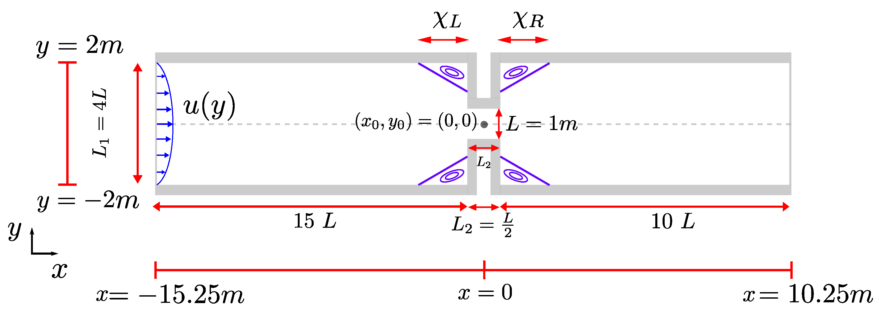
A sketch of the planar 4:1:4 contraction-expansion geometry is illustrated in Figure 15, where a parabolic profile is set at the inlet of the first channel, which will undergo through a contraction that is located at the centre of the domain. The main difference with respect to the planar 4:1 contraction geometry is that here, the contraction is almost immediately followed by an expansion. The inlet and outlet regions of the middle channel are exactly located at and , respectively.
Figure 15.
Domain representation: the planar 4:1:4 contraction-expansion geometry.
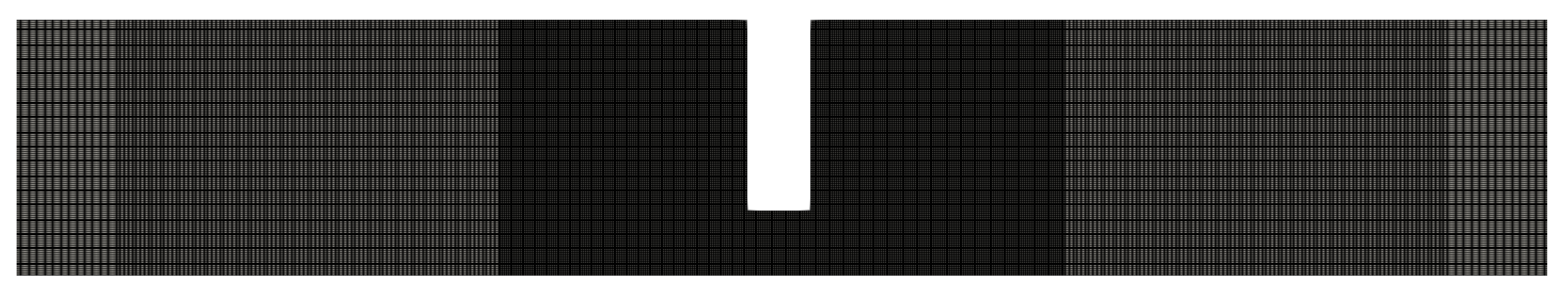
In our results of the mesh convergence analysis shown in Section 4.1.1, we concluded that we do not need to use uniform meshes with small cell size values in order to obtain high accurate solutions, since we observe that solutions from our meshes with localized refinements are similar to those solutions obtained in uniform meshes. Therefore, we will only focus on simulating flows using a refined mesh RMEC with the following specifications: the most refined part near the contraction region has cell size values , the second level of refinement has and the third one (whose cells cover mostly the regions near the inlet and outlet regions) . The inlet and outlet regions have are refined with cells of size . A graphical representation of the mesh RMEC used in our simulations is shown in Figure 16. As previously stated, we only simulate half of the domain since the flow is symmetric. Lastly, we use the same time-step value in all the simulations.
Figure 16.
Refined mesh RMEC used in OpenFoam/rheoTool (3 refinement levels) for the planar 4:1:4 contraction-expansion problem.
Figure 16.
Refined mesh RMEC used in OpenFoam/rheoTool (3 refinement levels) for the planar 4:1:4 contraction-expansion problem.
Similarly to the results shown in Section 4.1.2, we carry out numerical simulations of the MBM model in the planar 4:1:4 contraction-expansion geometry of fluids with exactly the same parameter values reported in Table 2. We are also interested in studying two cases: a strong-hardening fluid (with reformation parameter value ) and a moderate-hardening fluid ().
In these kinds of geometries, two corner vortexes will be formed: one at the upstream channel (with vortex size ) and another one at the downstream one (). In order to avoid being too repetitive with respect to the previous section, we will only limit ourselves to study the transient and steady-state behaviour of the vortexes sizes. We strongly encourage the reader to see our previous work [28], where we report the centreline axial profiles for the velocity, viscosity and components of the stress tensor for these kinds of fluids using the MBM model with and . We observed that the corner vortex from the upstream channel will decrease in size if the Reynolds number is being increased. On the other hand, we observe the opposite behaviour for the vortex of the downstream channel: an increase in will lead to a slight increase in . In the present work, we will intend to explain what is the cause of these phenomena, which will provide an insight behind the mechanism of formation of vortexes for these type of fluids.
4.2.1. Vortex dynamics: transient and steady-state behaviour
Firstly, we focus on studying the transient solutions of the upstream vortex size (the vortex located to the left of the geometry, found in the corner of upstream channel before the contraction region) for both and , see Figure 17a). The behaviour seen here resembles to that of the planar 4:1 contraction-expansion geometry (see Figure 11): we observe an overshoot at small times, which is followed by a plateau, after which the vortex reaches its steady state value. In addition, similarly to what we observe in the 4:1 case, the overshoot tends to be displaced from left to right as we increase the Reynolds number. In all the cases, a maximum value is observed, but the highest value is observed for the case (dashed line). Moreover, the transient curves also seem to be more stable for the creeping-flow case (). As mentioned earlier, another noticeable observation is that the steady vortex size value is decreased when the Reynolds number increases. The main difference between the strong- and moderate-hardening cases is that the upstream vortex size is slightly larger for the latter: with fixed, a value of is obtained with , while the vortex size is for the strong-hardening case (). Similar analysis is made when , where we also obtain a higher value of vortex size for the moderate-hardening case () compared to the value obtained with ().
On the other hand, we have the transient curves of the downstream vortex size (the vortex located to the right of the geometry, found in the corner of the downstream channel after the contraction region) shown in Figure 17b. The behaviour of these curves seem to be similar with respect to the curves of the upstream vortex (overshoot seen at small times and displacement of the curves from left to right as we increase the Reynolds number). However, there are two noticeable differences: 1) as is increased, the maximum value of each curve is also increased and 2) the steady-state value of the vortex size slightly increases if the inertial effects grow. For instance, if we focus on the moderate-hardening case (), the vortex size value for the creeping-flow is , while a value of is obtained with , resulting in a error difference between them. A similar behaviour is seen with : the vortex size is bigger for the inertial flow () compared to the case (), with a error difference. It can also be noticed that the vortexes sizes are also larger for the moderate-hardening case compared to the strong-hardening case, which is in agreement with our results from the planar-contraction 4:1 at low shown in Section 4.1.3.
This difference in vortex sizes at both creeping- and inertial flows predicted by our numerical results still need to be validated by experiments. Since those experiments do not exist yet, we will study the fluidity and first normal stress differences in the contraction/expansion regions for each of the scenarios shown above.
In Figure 18, we present the results for the strong-hardening scenario. At the top of the figure, we display the streamlines for both the creeping-flow (on the left) and inertial (on the right) cases. The creeping-flow case exhibits an interesting phenomenon of upstream growth and downstream shrinkage. This behavior was initially documented in [26] for the MBM model at and , as depicted in Figure 7 of their paper. Remarkably, our results for the case align with this finding. However, it’s worth noting that in [26], the size disparity between the vortexes is much more pronounced. In their case, the upstream vortex is nearly three times larger than the downstream one. To gain deeper insights into this difference, we analyze the fluidity and profiles displayed below.
From our fluidity profiles, it’s evident that fluidity bands spread outwards from the corner of the entrant region, consistent with our observations in Section 4.1.3. Interestingly, this behavior is observed for both and , but the creeping-flow case exhibits a broader coverage of fluidity bands near the upper corner of the upstream channel. This contrasts with the findings of Lopez-Aguilar et al. [26], who studied the moderate-hardening case of the MBM model with and (neglecting convective terms). They reported that the profiles are semi-symmetric at low Deborah numbers, becoming less symmetric with increasing , resulting in higher fluidity values near the salient region of the upstream channel or the entrant region of the contraction channel.
However, our results display a different trend: higher fluidity values (indicating viscosity thinning) are convected from the contraction region towards the downstream channel. This divergence in behavior may explain why the difference in size between the upstream and downstream vortices is more pronounced in [26] than in our results illustrated in Figure 18. Clearly, even when inertial effects are minimal (), convective terms in all governing equations play a pivotal role in geometries of this nature and cannot be entirely disregarded.
As we know, the fluidity also has an effect on the normal stress differences, and thus, we report our profiles at the bottom of Figure 18. If we focus first on studying the upstream channel, we will notice that negative normal stress difference dominate near the corner of the entrant region. Similarly to the fluidity profiles, large values of are observed near the corners in the salient region of the contraction channel. In addition, our results report clouds (of green colour) of middle-to-high values of () near the entrant region of the downstream channel, which are more larger compared to the clouds reported in [26]. This again would explain why the downstream vortex predicted by our simulations with inertia is much larger compared to the vortex size predicted in [26] with .
It’s worth noting that our profiles denoted as closely resemble those presented in Lopez-Aguilar’s study [26]. However, their findings fail to anticipate the high elasticity zone observed near the upper wall of the contraction region (the red-yellow zone). This discrepancy can be attributed to the significant influence of convection and inertia included in our governing equations. Additionally, our use of a rectangular mesh (as opposed to the rounded mesh employed in [26]) could also contribute to these disparities. We will study these differences in greater detail in the subsequent discussion of our results.
Lastly, we also decided to carry out numerical simulations for the moderating-hardening case with (see Figure 19), where the difference between the upstream/downstream vortexes is more noticeable. For instance, for the creeping flow case, we obtain an upstream vortex size value of while the downstream vortex size is , resulting in a error difference between the values. On the other hand, for the case , we observe a higher error difference: , where the upstream vortex and downstream vortex sizes are and , respectively. In contrast, the error difference between the upstream/downstream vortexes when (from Figure 18) are for the creeping-flow and when . Lopez-Aguilar et al. [26] also carried out inertialess simulations for the moderate-hardening case with fixed, and they reported a significant shrinkage in the downstream vortex, which almost becomes negligible compared to upstream vortex. Our numerical simulations do also predict the shrinkage in the downstream vortex for the creeping flow case, that goes from a value of (when ) to (when ). The main difference between our simulations with respect the results reported in [26] is that the size of the downstream vortex remains considerable in our simulations. In addition, Lopez-Aguilar et al. also observed an increase in upstream vortex size when the viscoelastic effects grow, which is the opposite of what we see in our results: we obtain a value of when and a value of when .
Although it is worth mentioning that Lopez-Aguilar et al. simulated these type of flows using a rounded-corner contraction/expansion mesh, which could partially explain why the downstream corner vortex shrinks considerably, we also simulated in rheoTool the creeping-flow case with fixed for two values of Deborah number ( and ), while ignoring the convective term of the fluidity equation from equation (9). These results can be found in Figure 20, where it is evident that the fluidity and profiles are symmetric, leading to upstream/downstream corner vortexes of similar size, which is in excellent agreement with the observations reported by Lopez-Aguilar et al. [26,27]. From the fluidity profiles, we can observe regions of high fluidity in the corners of the contraction channel, which are caused due to the consideration of a rectangular mesh (unlike the corner-rounded mesh used in [26,27]). For the case , the fluidity profiles are almost symmetric, but more importantly, it can be easily seen that the fluidity is not strongly convected towards the downstream channel compared to the profiles with the inclusion of the fluidity convective term previously shown in Figure 18. In addition, the shrinkage of the downstream vortex is more evident for the simulations without the term ; for instance, with both and fixed, the downstream corner vortex size obtained considering convection of fluidity is , while a value of is seen without convection of fluidity. Lastly, our simulation without the term predict a larger value of upstream corner vortex () compared to our simulation that does consider convection of ().
5. Conclusions
In this study, we present the numerical results obtained by integrating the thixotropic-viscoelastic Modified-Bautista-Manero (MBM) model into the OpenFoam/rheoTool framework. In the initial sections, we provide an overview of the system and outline the governing equations used in our simulations. Additionally, we introduce the MBM model, offering insights into the physical interpretations of its parameters, the dimensionless groups derived from the model, its predictive capabilities in terms of rheological behavior, and its strengths and weaknesses. The original Bautista-Manero-Puig (BMP) model, which was already part of the rheoTool version 5.0, was found to yield unrealistic extensional viscosity values in extensional flows. Thus, in this work, we implement the MBM model to rectify these issues associated with the BMP model.
We focused on simulating thixotropic-viscoelastic flows in two common geometries: the planar 4:1 contraction and 4:1:4 contraction-expansion. Using uniform and locally refined meshes, we carry out a mesh convergence analysis and we found that the solutions obtained from the locally refined meshes are very close to the results predicted using uniform meshes with very small cell size values.
In all of our simulations, we explored two distinct fluid scenarios:
- Strong-Hardening Case: This involves a fluid that exhibits rapid structural recovery, characterized by and a swift restoration of viscosity.
- Moderate-Hardening Case: In this case, we dealt with a fluid exhibiting slightly slower structural recovery, with .
Both of these cases were simulated using varying Deborah numbers (), and our findings revealed that the steady-state centerline profiles align closely with previously reported results in the literature.
We also performed numerical simulations using the MBM model with a non-zero Reynolds number in the rheoTool software. This choice was motivated by the fact that the majority of research in the literature on thixotropic-viscoelastic flows does not take into account inertia or fluidity convection. To gain insight into the impact of the Reynolds number on viscosity and the polymeric stress tensor, we compared our results to the case without inertia. Our findings revealed that a higher inertia leads to a slightly greater reduction in the structural integrity (and consequently, viscosity) near the contraction region at the centerline. Furthermore, as anticipated, the normal stresses exhibit an inverse relationship with the Reynolds number.
In addition, we have obtained numerical results for both transient and steady-state solutions related to corner vortex behavior. Specifically, we investigated the corner vortex in a planar 4:1 contraction geometry and the upstream/downstream corner vortexes in a planar 4:1:4 contraction-expansion geometry. Our study focused on understanding how the interplay of viscoelasticity, inertia, and thixotropy influences these vortex phenomena. In the case of the planar 4:1 contraction geometry, we plotted the relationship between vortex size () and the Deborah number. In both the scenarios of strong and moderate hardening, we observed a decrease in at low Deborah numbers. However, as we increased the Deborah number, there was a rapid increase in (refer to Figure 10). Our findings align with previously reported works in the literature (see references [25,33]).
Furthermore, the use of the log-conformation approach enabled us to simulate flows at moderately high Deborah numbers. This allowed us to explore the behavior of over extended periods, revealing that reaching a steady state takes significantly longer when Deborah number () is high. We derived three dimensionless numbers, the viscoelastic Mach number M (proportional to the square root of ), the elasticity number () and the thixoelastic number , and we found that the vortex size increases with the increase of both M and E. More importantly, we show that vortex-enhancement is seen when the elastic effects are dominant at low flow rates, specially if the stress relaxation time is slower compared to the structural recovery of the fluid (i.e., ). On the other hand, vortex-inhibition is observed when the inertial effects increase (decrease in ) and if elasticity is no longer dominant or if it is of the same order of magnitude of the thixotropic and inertial effects.
Our results obtained using the MBM model were also compared with those obtained using the exponential-PTT (EPTT) model, a non-thixotropic rubber network-based polymer model, where we show that the thixotropic model can provide us more rich information regarding the evolution of the internal structure of the fluid. For instance, the fluidity (inverse of viscosity) profiles were used to illustrate that bands of low viscosity spread out from the contraction region and manage to reach the top wall of the upstream channel, which could help to understand the mechanism of vortex-enhancement seen in our results at high .
Laslty, our study includes results obtained from numerical simulations conducted in a planar 4:1:4 contraction-expansion geometry. Our findings for steady-state conditions in the context of creeping flow align with previously reported research (Lopez et al., 2014; Lopez et al., 2015). Furthermore, our simulations involving a non-zero Reynolds number, especially concerning transient and steady-state solutions for corner vortex size, yield novel insights and highly accurate data in this geometry. Notably, we demonstrate that increasing inertial effects leads to inhibition of vortex formation in the upstream region and a slight enhancement of vortexes in the downstream channel. It would be beneficial to conduct experiments on thixotropic-viscoelastic flows with inertia to validate our discoveries. In addition, we highlight the significant impact of introducing convection of fluidity, represented as , into the fluidity profiles and its effects on the upstream and downstream corner vortex sizes. Specifically, we observe the breakdown of symmetry in the fluidity profiles due to strong fluidity convection toward the downstream channel, as well as a less pronounced reduction in the size of the downstream corner vortex compared to cases without fluidity convection.
In our future research, it is essential to expand our exploration of fluid behavior to encompass more extensive ranges of Deborah and Reynolds numbers. We are particularly interested in investigating these behaviors within the context of the planar 4:1:4 contraction-expansion geometry. Lopez-Aguilar et al. [26] have already made notable contributions to this field, identifying a critical Deborah number of for the MBM model. To push beyond these constraints, they introduced two related models: and , which incorporate elasticity and solvent effects into the fluidity evolution equation. These models enabled them to simulate flows up to . Therefore, our next step involves integrating these models, as well as complex ones that combine the EPTT and MBM models [26,47], into the rheoTool framework. This will enable us to simulate flows under inertial conditions without problems of numerical stability. Furthermore, we aim to investigate whether the conditions previously identified in Section 4.1.4 for the planar 4:1 contraction geometry (specifically, the observation of vortex enhancement when ) hold true for the planar 4:1:4 contraction-expansion geometry, both in upstream and downstream vortex scenarios.
Author Contributions
Conceptualization, H.A.C.S., M.S.B.A., J.B., and A.C.; methodology, H.A.C.S., M.S.B.A., J.B., C.F., L.F.F. and A.C.; software, H.A.C.S. and M.S.B.A.; validation, H.A.C.S., M.S.B.A. and C.F.; formal analysis, H.A.C.S., J.B., C.F. and L.F.F.; investigation, H.A.C.S. and C.F.; data curation, H.A.C.S. and M.S.B.A.; writing—original draft preparation, H.A.C.S.; writing—review and editing, H.A.C.S., J.B., C.F. and L.F.F.; visualization, H.A.C.S., M.S.B.A. and J.B.; supervision, A.C. and C.F.; project administration, H.A.C.S., C.F. and A.C.; funding acquisition, C.F. and A.C. All authors have read and agreed to the published version of the manuscript.
Funding
All authors thank the financial support from the São Paulo Research Foundation (FAPESP) grants 2013/07375-0 and 2020/02990-1. This research was also funded by FCT (Fundação para a Ciência e a Tecnologia) and CMAT (Centre of Mathematics of the University of Minho) projects UIDB/00013/2020 and UIDP/00013/2020, FCT project 2022.06672.PTDC and contract 2022.00753.CEECIND.
Acknowledgments
H. A. Castillo-Sánchez and A. Castelo acknowledge the support by ICMC - Instituto de Ciências Matemáticas e de Computação, Departamento de Matemática e Estatística, USP, São Carlos, SP. M.S.B. de Araújo acknowledge the support by UFPA - Universidade Federal do Pará, Instituto de Ciências Exatas e Naturais. J. Bertoco acknowledges the support by CMCC - Centro de Matemática, Computação e Cognição, UFABC. M.S.B. de Araújo acknowledges the support by UFPA - Universidade Federal do Pará, Instituto de Ciências Exatas e Naturais. L.L. Ferrás would like to thank FCT (Fundação para a Ciência e a Tecnologia) for financial support through CMAT (Centre of Mathematics of the University of Minho) projects UIDB/00013/2020 and UIDP/00013/2020 and would also like to thank FCT for the funding of project 2022.06672.PTDC. C. Fernandes acknowledges the support by FEDER funds through the COMPETE 2020 Programme and National Funds through FCT (Portuguese Foundation for Science and Technology) under the contract FCT/2022.00753.CEECIND.
Conflicts of Interest
The authors declare no conflict of interest.
Abbreviations
The following abbreviations are used in this manuscript:
| MBM | Modified-Bautista-Manero |
| BMP | Bautista-Manero Puig |
| CFD | Computational Fluid Dynamics |
| PTT | Phan-Tien-Tanner |
| EPTT | Exponential Phan-Tien-Tanner |
| UCM | Upper-Convected-Maxwell |
| GNF | Generalized Newtonian Fluids |
| FVM | Finite-Volume-Method |
| BSD | Both-sides-diffusion |
| iBSD | Improved Both-sides-diffusion |
| DILU | Simplified Diagonal-based Incomplete LU preconditioner |
| PETSc | Portable, Extensible Toolkik for Scientific Computation |
| PCG | Conjugated Preconditioned Gradients |
| Bi-CGSTAB | Bi-Conjugate Gradient Stabilized |
| DIC | Diagonal-based Incomplete Cholesky |
| CUBISTA | Convergent and Universally Bounded Interpolation Scheme for the Treatment of Advection |
References
- White, J.L.; Metzner, A.B. Development of constitutive equations for polymeric melts and solutions. Journal of Applied Polymer Science 1963, 7, 1867–1889. [Google Scholar] [CrossRef]
- Oldroyd, J.G.; Wilson, A.H. On the formulation of rheological equations of state. Proceedings of the Royal Society of London. Series A. Mathematical and Physical Sciences 1950, 200, 523–541. [Google Scholar] [CrossRef]
- Thien, N.P.; Tanner, R.I. A new constitutive equation derived from network theory. Journal of Non-Newtonian Fluid Mechanics 1977, 2, 353–365. [Google Scholar] [CrossRef]
- Giesekus, H. Die Elastizität von Flüssigkeiten. Rheologica Acta 1966, 5, 29–35. [Google Scholar] [CrossRef]
- Bird, R. Dynamics of Polymeric Liquids, Volume 1: Fluid Mechanics; Dynamics of Polymeric Liquids, Wiley, 1987.
- Alves, M.; Oliveira, P.; Pinho, F. Numerical Methods for Viscoelastic Fluid Flows. Annual Review of Fluid Mechanics 2021, 53, 509–541. [Google Scholar] [CrossRef]
- Yesilata, B.; Clasen, C.; McKinley, G. Nonlinear shear and extensional flow dynamics of wormlike surfactant solutions. Journal of Non-Newtonian Fluid Mechanics 2006, 133, 73–90. [Google Scholar] [CrossRef]
- Fernandes, C.; Faroughi, S.A.; Carneiro, O.S.; Nóbrega, J.M.; McKinley, G.H. Fully-resolved simulations of particle-laden viscoelastic fluids using an immersed boundary method. Journal of Non-Newtonian Fluid Mechanics 2019, 266, 80–94. [Google Scholar] [CrossRef]
- Fernandes, C.; Faroughi, S.A.; Ribeiro, R.; Isabel, A.; McKinley, G.H. Finite volume simulations of particle-laden viscoelastic fluid flows: application to hydraulic fracture processes. Engineering with Computers 2022, 38, 5395–5421. [Google Scholar] [CrossRef]
- Chávez-Miyauchi, T.E.; Firoozabadi, A.; Fuller, G.G. Nonmonotonic Elasticity of the Crude Oil–Brine Interface in Relation to Improved Oil Recovery. Langmuir 2016, 32, 2192–2198. [Google Scholar] [CrossRef]
- Nodoushan, E.J.; Yi, T.; Lee, Y.J.; Kim, N. Wormlike Micellar Solutions, Beyond the Chemical Enhanced Oil Recovery Restrictions. Fluids 2019, 4, 173. [Google Scholar] [CrossRef]
- Frigaard, I.A.; Paso, K.G.; de Souza Mendes, P.R. Bingham’s model in the oil and gas industry. Rheologica Acta 2017, 56, 259–282. [Google Scholar] [CrossRef]
- Fink, J. Water-based chemicals and technology for drilling, completion, and workover fluids; Gulf Professional Publishing, 2015.
- Spagnolie, S.E. Complex fluids in biological systems: experiment, theory, and computation; Vol. 6, Springer, 2015. [CrossRef]
- Moreno, L.; Calderas, F.; Sanchez-Olivares, G.; Medina-Torres, L.; Sanchez-Solis, A.; Manero, O. Effect of cholesterol and triglycerides levels on the rheological behavior of human blood. Korea-Australia Rheology Journal 2015, 27, 1–10. [Google Scholar] [CrossRef]
- Gallegos, C.; Franco, J.M. Rheology of food, cosmetics and pharmaceuticals. Current Opinion in Colloid & Interface Science 1999, 4, 288–293. [Google Scholar] [CrossRef]
- Eley, R.R. Applied rheology in the protective and decorative coatings industry. Rheology Reviews 2005. [Google Scholar]
- Larson, R.G. The structure and rheology of complex fluids; Topics in Chemical Engineering, Oxford University Press, 1998.
- Bautista, F.; De Santos, J.M.; Puig, J.E.; Manero, O. Understanding thixotropic and antithixotropic behavior of viscoelastic micellar solutions and liquid crystalline dispersions. I. The model. Journal of Non-Newtonian Fluid Mechanics 1999, 80, 93–113. [Google Scholar] [CrossRef]
- Calderas, F.; Herrera-Valencia, E.E.; Sanchez-Solis, A.; Manero, O.; Medina-Torres, L.; Renteria, A.; Sanchez-Olivares, G. On the yield stress of complex materials. Korea-Australia Rheology Journal 2013, 25, 233–242. [Google Scholar] [CrossRef]
- Bautista, F.; Soltero, J.F.A.; Pérez-López, J.H.; Puig, J.E.; Manero, O. On the shear banding flow of elongated micellar solutions. Journal of Non-Newtonian Fluid Mechanics 2000, 94, 57–66. [Google Scholar] [CrossRef]
- Vasquez, P.A.; McKinley, G.H.; Cook, L.P. A network scission model for wormlike micellar solutions: I. Model formulation and viscometric flow predictions. Journal of Non-Newtonian Fluid Mechanics 2007, 144, 122–139. [Google Scholar] [CrossRef]
- Boek, E.S.; Padding, J.T.; Anderson, V.J.; Tardy, P.M.J.; Crawshaw, J.P.; Pearson, J.R.A. Constitutive equations for extensional flow of wormlike micelles: stability analysis of the Bautista–Manero model. Journal of Non-Newtonian Fluid Mechanics 2005, 126, 39–46. [Google Scholar] [CrossRef]
- Pimenta, F.; Alves, M.A. RheoTool. https://github.com/fppimenta/rheoTool, 2017.
- Tamaddon Jahromi, H.R.; Webster, M.F.; Aguayo, J.P.; Manero, O. Numerical investigation of transient contraction flows for worm-like micellar systems using Bautista–Manero models. Journal of Non-Newtonian Fluid Mechanics 2011, 166, 102–117. [Google Scholar] [CrossRef]
- López-Aguilar, J.E.; Webster, M.F.; Tamaddon-Jahromi, H.R.; Manero, O. A new constitutive model for worm-like micellar systems – Numerical simulation of confined contraction–expansion flows. Journal of Non-Newtonian Fluid Mechanics 2014, 204, 7–21. [Google Scholar] [CrossRef]
- López-Aguilar, J.E.; Webster, M.F.; Tamaddon-Jahromi, H.R.; Manero, O. High-Weissenberg predictions for micellar fluids in contraction–expansion flows. Journal of Non-Newtonian Fluid Mechanics 2015, 222, 190–208. [Google Scholar] [CrossRef]
- Castillo-Sánchez, H.A.; Bertoco, J.; de Araújo, M.S.; Castelo, A. Numerical simulation of thixotropic–viscoelastic models for structured fluids in hierarchical grids. Computers & Fluids 2023, 266, 106045. [Google Scholar] [CrossRef]
- Castelo, A.; Afonso, A.M.; De Souza Bezerra, W. A Hierarchical Grid Solver for Simulation of Flows of Complex Fluids. Polymers 2021, 13, 3168. [Google Scholar] [CrossRef]
- Sousa, F.S.; Lages, C.F.; Ansoni, J.L.; Castelo, A.; Simao, A. A finite difference method with meshless interpolation for incompressible flows in non-graded tree-based grids. Journal of Computational Physics 2019, 396, 848–866. [Google Scholar] [CrossRef]
- Fredrickson, A.G. A model for the thixotropy of suspensions. AIChe Journal 1970, 16, 436–441. [Google Scholar] [CrossRef]
- Castillo, H.A.; Wilson, H.J. Elastic instabilities in pressure-driven channel flow of thixotropic-viscoelasto-plastic fluids. Journal of Non-Newtonian Fluid Mechanics 2018, 261, 10–24. [Google Scholar] [CrossRef]
- Pimenta, F.; Alves, M.A. Stabilization of an open-source finite-volume solver for viscoelastic fluid flows. Journal of Non-Newtonian Fluid Mechanics 2017, 239, 85–104. [Google Scholar] [CrossRef]
- Fattal, R.; Kupferman, R. Constitutive laws for the matrix-logarithm of the conformation tensor. Journal of Non-Newtonian Fluid Mechanics 2004, 123, 281–285. [Google Scholar] [CrossRef]
- Afonso, A.; Oliveira, P.J.; Pinho, F.T.; Alves, M.A. The log-conformation tensor approach in the finite-volume method framework. Journal of Non-Newtonian Fluid Mechanics 2009, 157, 55–65. [Google Scholar] [CrossRef]
- Ferrás, L.L.; Morgado, M.L.; Rebelo, M.; McKinley, G.H.; Afonso, A. A generalised Phan–Thien—Tanner model. Journal of Non-Newtonian Fluid Mechanics 2019, 269, 88–99. [Google Scholar] [CrossRef]
- Phan-Thien, N. A Nonlinear Network Viscoelastic Model. Journal of Rheology 1978, 22, 259–283. [Google Scholar] [CrossRef]
- Rhie, C.M.; Chow, W.L. Numerical study of turbulent flow past an isolated airfol with trailing edge separation. AIAA Journal 1983, 21, 1525–1532. [Google Scholar] [CrossRef]
- Fernandes, C.; Araújo, M.S.B.; Ferrás, L.L.; Miguel Nóbrega, J. Improved both sides diffusion (iBSD): A new and straightforward stabilization approach for viscoelastic fluid flows. Journal of Non-Newtonian Fluid Mechanics 2017, 249, 63–78. [Google Scholar] [CrossRef]
- PETSc. Portable, Extensible Toolkit for Scientific Computation, 1991. https://petsc.org/release/.
- Alves, M.A.; Oliveira, P.J.; Pinho, F.T. A convergent and universally bounded interpolation scheme for the treatment of advection. International Journal for Numerical Methods in Fluids 2003, 41, 47–75. [Google Scholar] [CrossRef]
- OpenFOAM Foundation, OpenFOAM v8 User Guide, 2020. https://cfd.direct/openfoam/user-guide.
- van der Vorst, H.A. Bi-CGSTAB: A Fast and Smoothly Converging Variant of Bi-CG for the Simulation of Nonsymmetric Linear Systems. SIAM Journal on Scientific and Statistical Computing 1992, 13, 631–644. [Google Scholar] [CrossRef]
- Jacobs, D. Preconditioned conjugate gradient methods for solving systems of algebraic equations. Technical Report RD/L/N193/80, Central Electricity Research Laboratories, 1980.
- Owens, R.G.; Phillips, T.N. Computational rheology; World Scientific, 2002.
- Choi, H.C.; Song, J.H.; Yoo, J.Y. Numerical simulation of the planar contraction flow of a Giesekus fluid. Journal of Non-Newtonian Fluid Mechanics 1988, 29, 347–379. [Google Scholar] [CrossRef]
- López-Aguilar, J.E.; Webster, M.F.; Tamaddon-Jahromi, H.R.; Manero, O. Convoluted models and high-Weissenberg predictions for micellar thixotropic fluids in contraction–expansion flows. Journal of Non-Newtonian Fluid Mechanics 2016, 232, 55–66. [Google Scholar] [CrossRef]
Figure 2.
Refined mesh RMI employed in the simulations of the planar 4:1 contraction benchmark problem. We used 3 refinement levels , and . In these regions and for , , for , and for , .
Figure 2.
Refined mesh RMI employed in the simulations of the planar 4:1 contraction benchmark problem. We used 3 refinement levels , and . In these regions and for , , for , and for , .
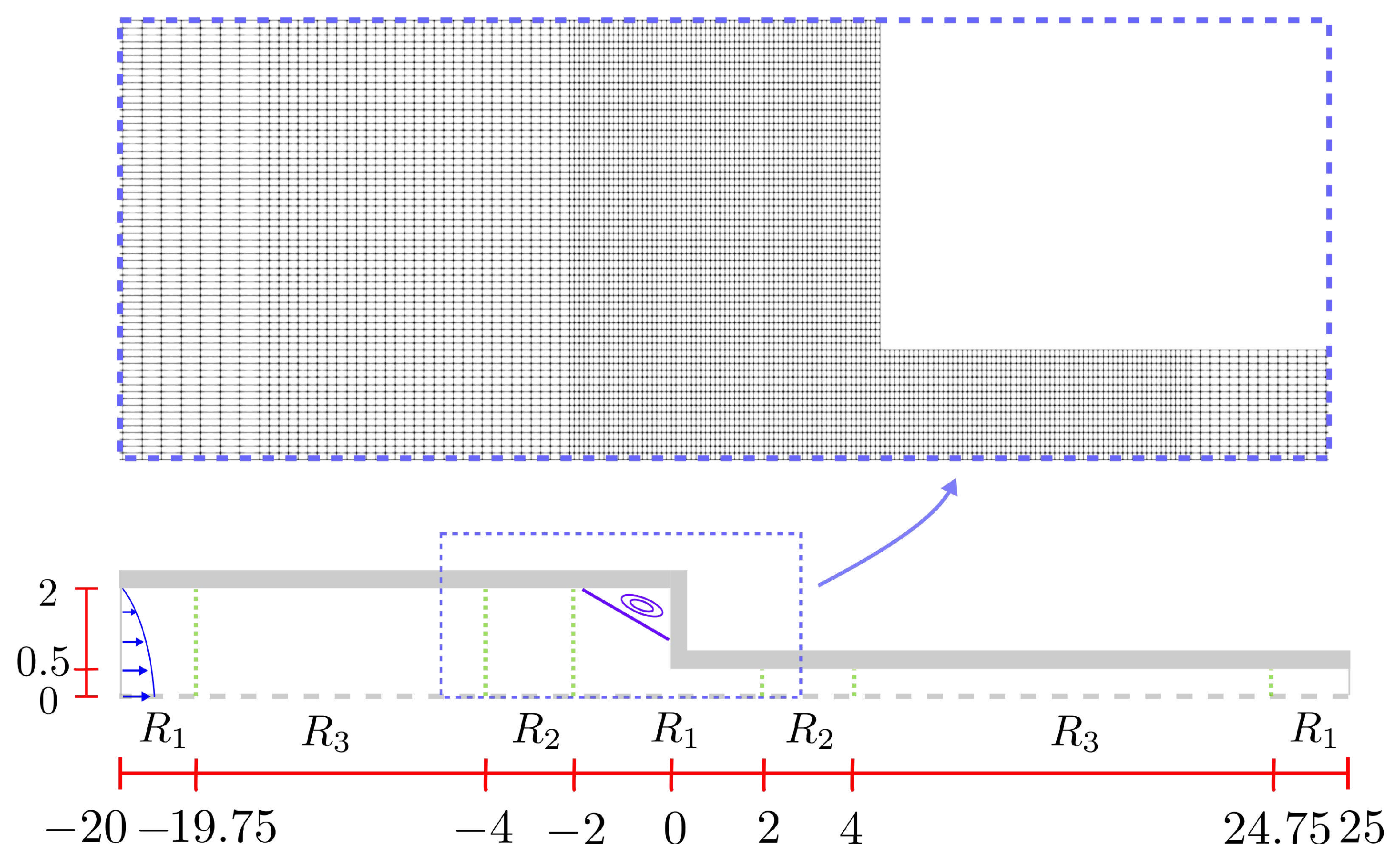
Figure 3.
Centreline axial velocity and viscosity profiles for the fluid with strong-hardening behaviour (). The numerical results of the planar 4:1 contraction flow problem using the MBM model were obtained for three uniform meshes (MI, MII and MIII) and two refined meshes (RMI and RMII). For these results, we fix the Deborah and the Reynolds numbers. The other fluid parameters used are shown in Table 2. Figure 3 and Figure 3 show zoomed regions of the wider curves shown in Figure 3 and Figure 3, respectively.
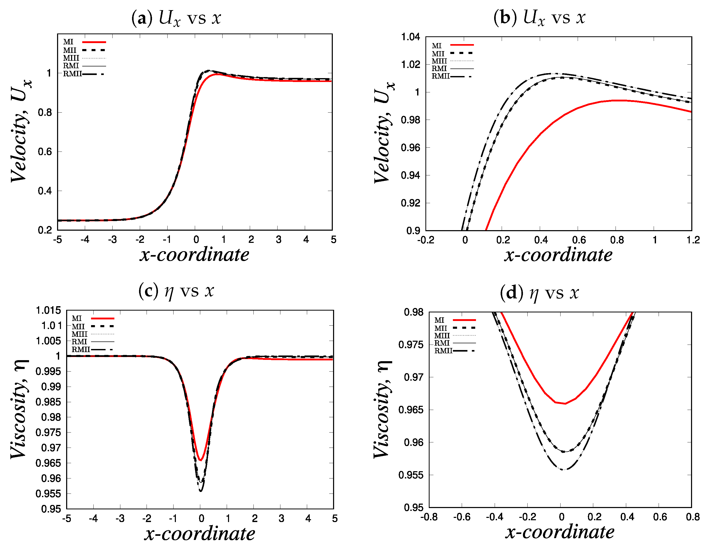
Figure 4.
Centreline normal stresses profiles for the fluid with strong-hardening behaviour (). The numerical results of the planar 4:1 contraction flow problem using the MBM model were obtained for three uniform meshes (MI, MII and MIII) and two refined meshes (RMI and RMII). For these results, we fix the Deborah and the Reynolds numbers. The other fluid parameters used are shown in Table 2. Figure 4 and Figure 4 show zoomed regions of the wider curves shown in Figure 4 and Figure 4, respectively.
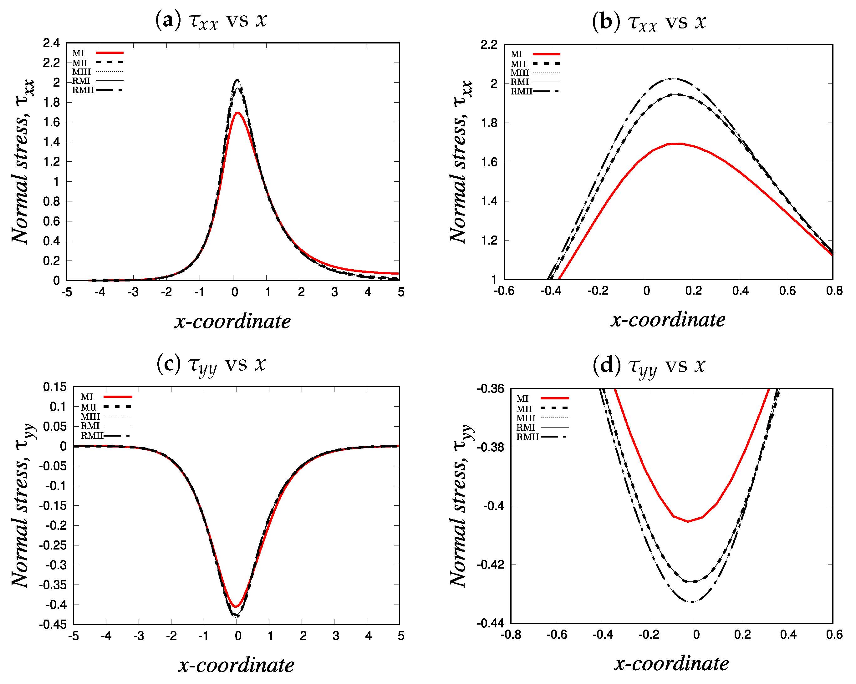
Figure 5.
Dimensionless centreline axial velocity profiles for the MBM fluid with strong- () and moderate-() hardening behaviours. For these results, we fix the Deborah number and simulate flows for three different Reynolds numbers: (red solid line), (dashed line) and (dotted line).
Figure 5.
Dimensionless centreline axial velocity profiles for the MBM fluid with strong- () and moderate-() hardening behaviours. For these results, we fix the Deborah number and simulate flows for three different Reynolds numbers: (red solid line), (dashed line) and (dotted line).
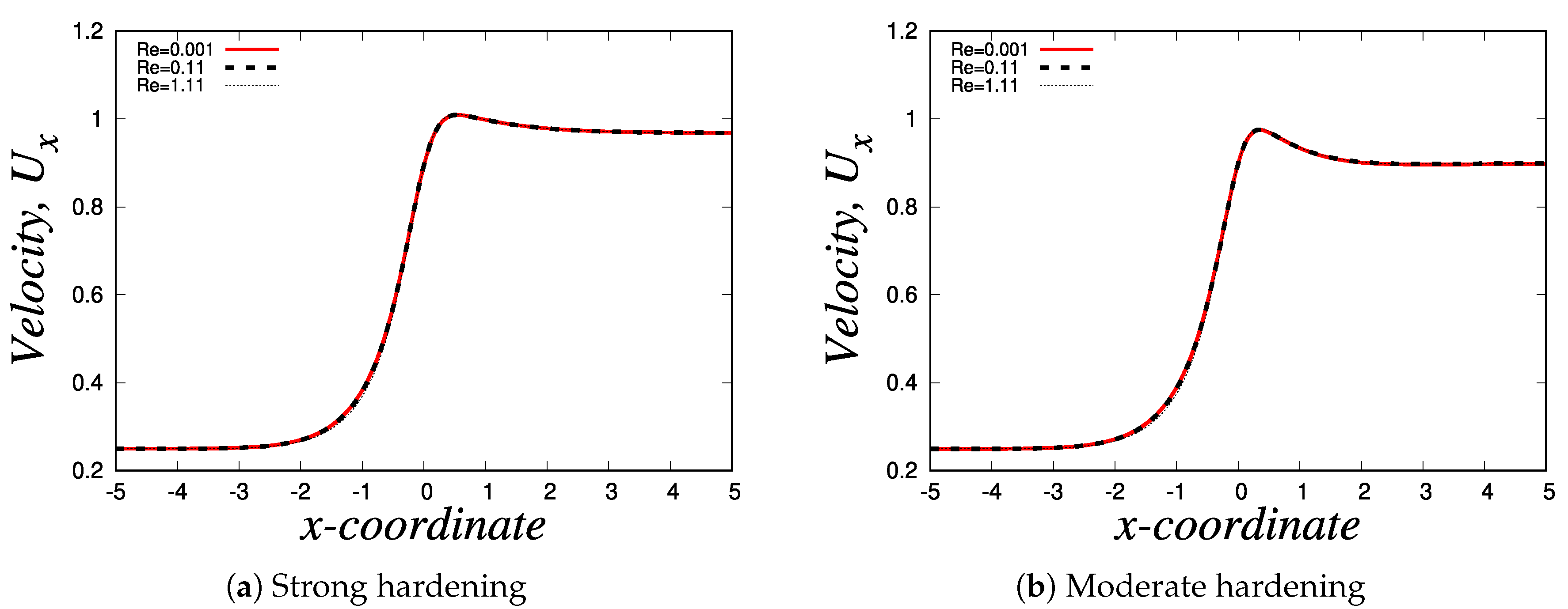
Figure 6.
Centreline axial viscosity and normal stresses profiles for the fluid with strong-hardening (with ) behaviour. In this plot, we show our numerical results of the planar 4:1 contraction flow problem for the MBM model using a refined mesh RM1. For these results, we fix the Deborah number and simulate flows for three different Reynolds numbers: (red solid line), (dashed line) and (dotted line). The fluid parameters used are shown in Table 2. Figure 6, Figure 6 and Figure 6 show zoomed regions of the wider curves shown in Figure 6, Figure 6 and Figure 6, respectively. All the profiles are in dimensionless form.
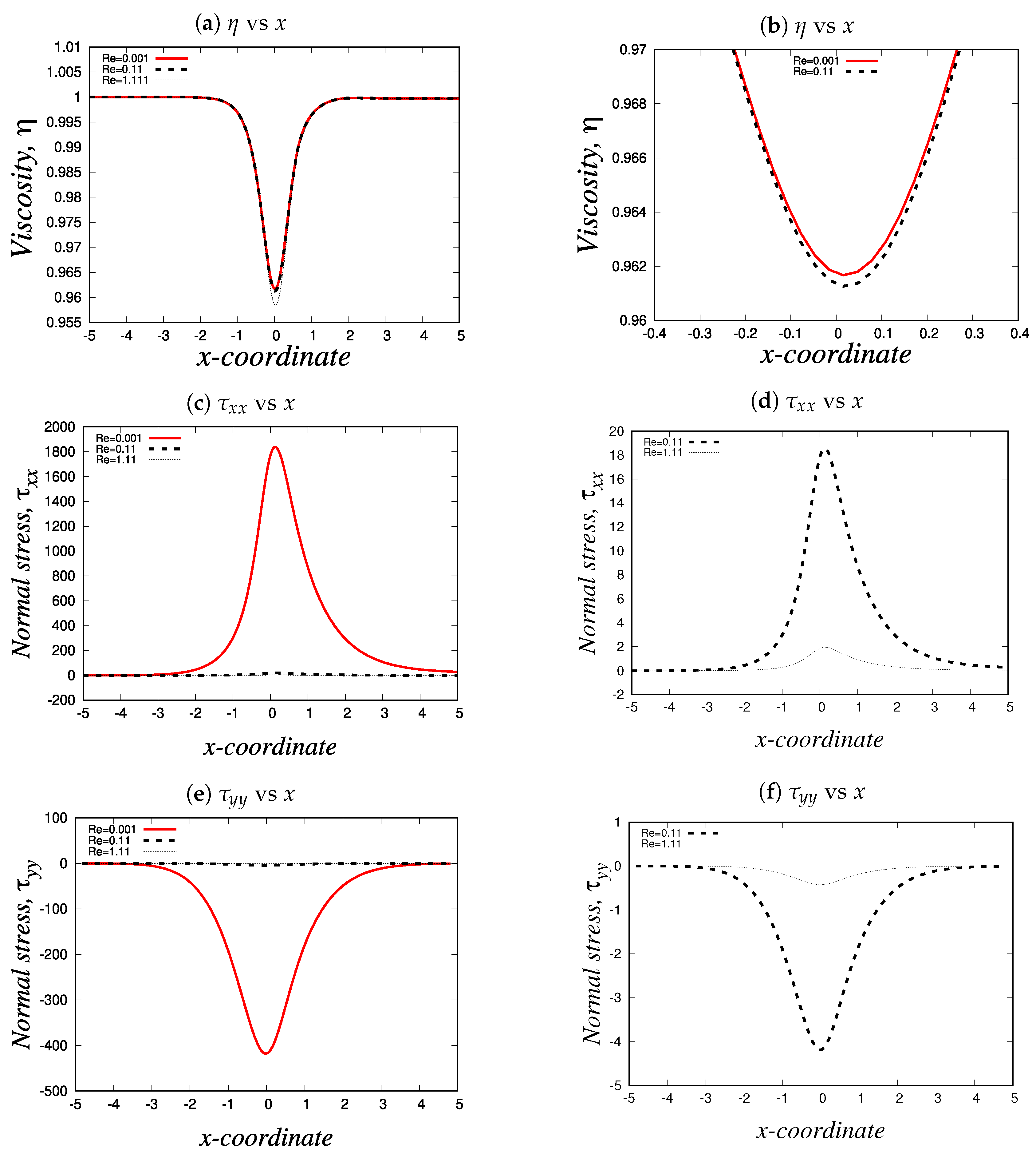
Figure 7.
Centreline axial viscosity and normal stresses profiles for the fluid with moderate-hardening behaviour. In this plot, we show our numerical results of the planar contraction 4:1 flow problem for the MBM model (with ) using a refined mesh. For these results, we fix the Weissenberg number and simulate flows for three different Reynolds numbers: (red solid line), (dashed line) and (dotted line). The fluid parameters used are shown in Table 2. Figure 7, Figure 7 and Figure 7 show zoomed regions of the wider curves shown in Figure 7, Figure 7 and Figure 7, respectively. All the profiles are in dimensionless form.
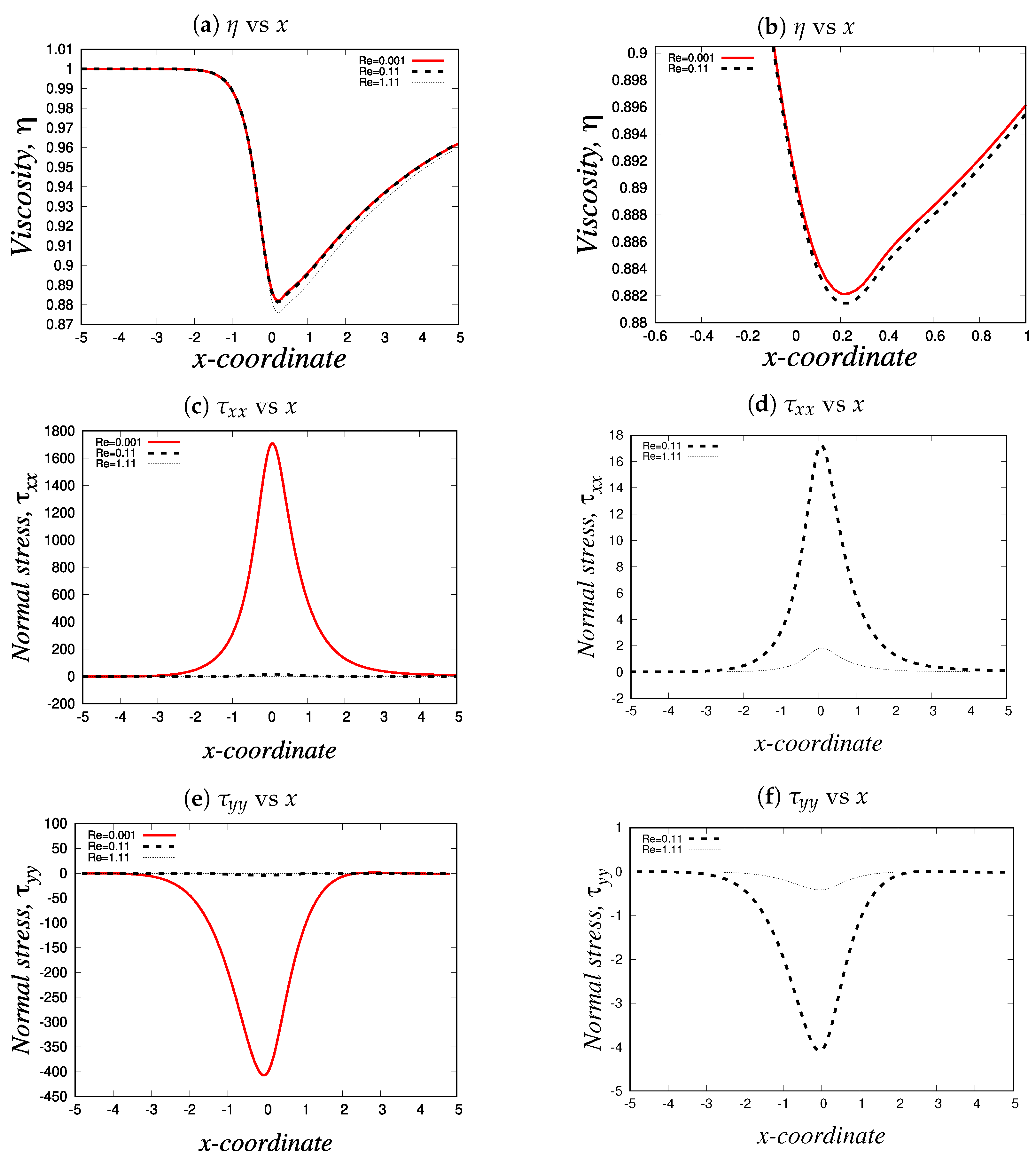
Figure 8.
Transient development of the fluidity profile for the moderate-hardening case () with and fixed.
Figure 8.
Transient development of the fluidity profile for the moderate-hardening case () with and fixed.

Figure 9.
Transient development of the fluidity profile for the strong-hardening case () with and fixed.
Figure 9.
Transient development of the fluidity profile for the strong-hardening case () with and fixed.
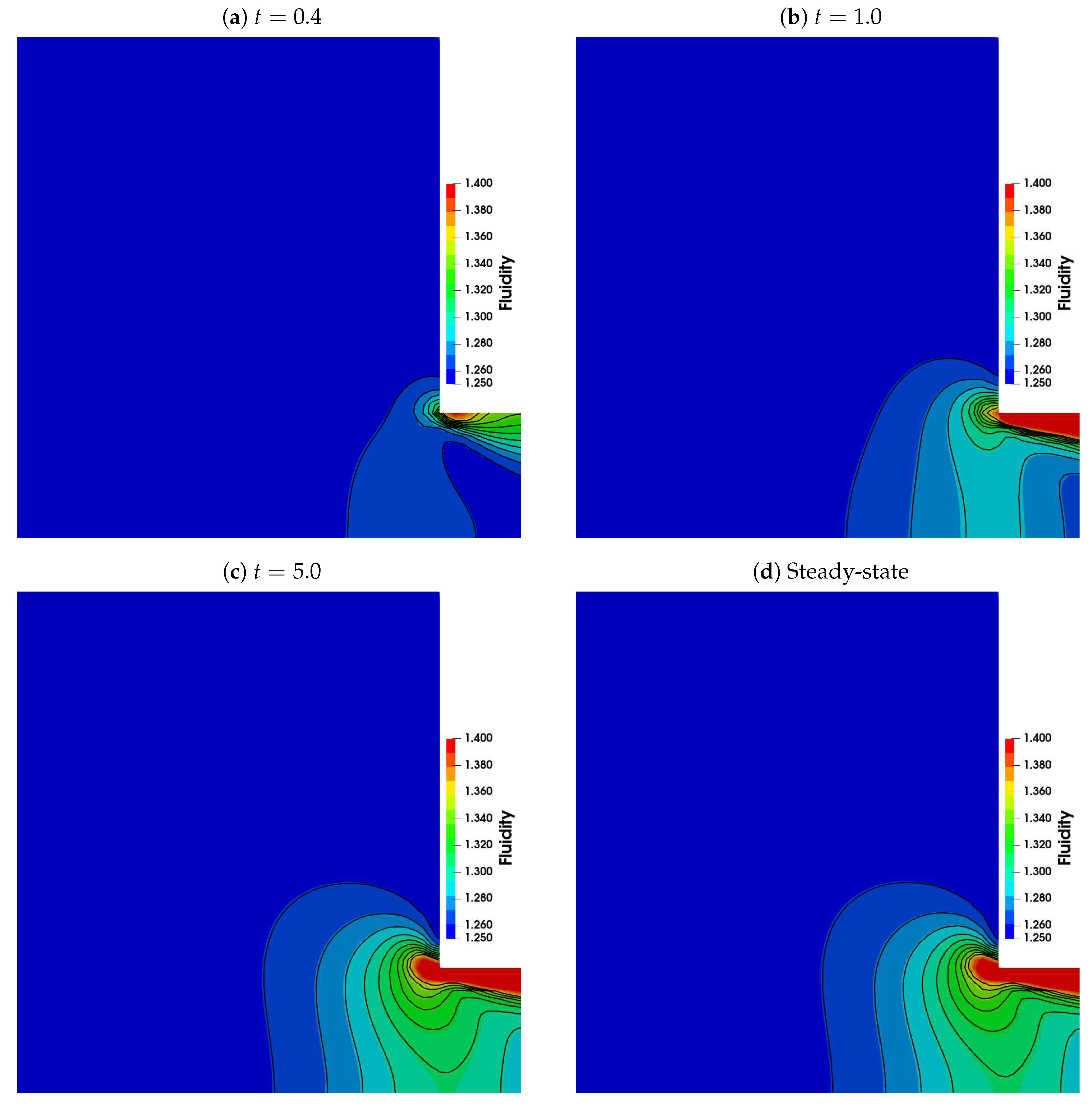
Figure 10.
Evolution of the corner vortex size, , as a function of the Deborah number, . The strong-hardening curves for cases of the MBM model () and the EPTT model () are found in the left, while the curves for the moderate-hardening cases of the MBM model () and the EPTT model () are located to the right. For each of these cases, we study the effect of the Reynolds number on the vortex size. From top to bottom, the is being increased.
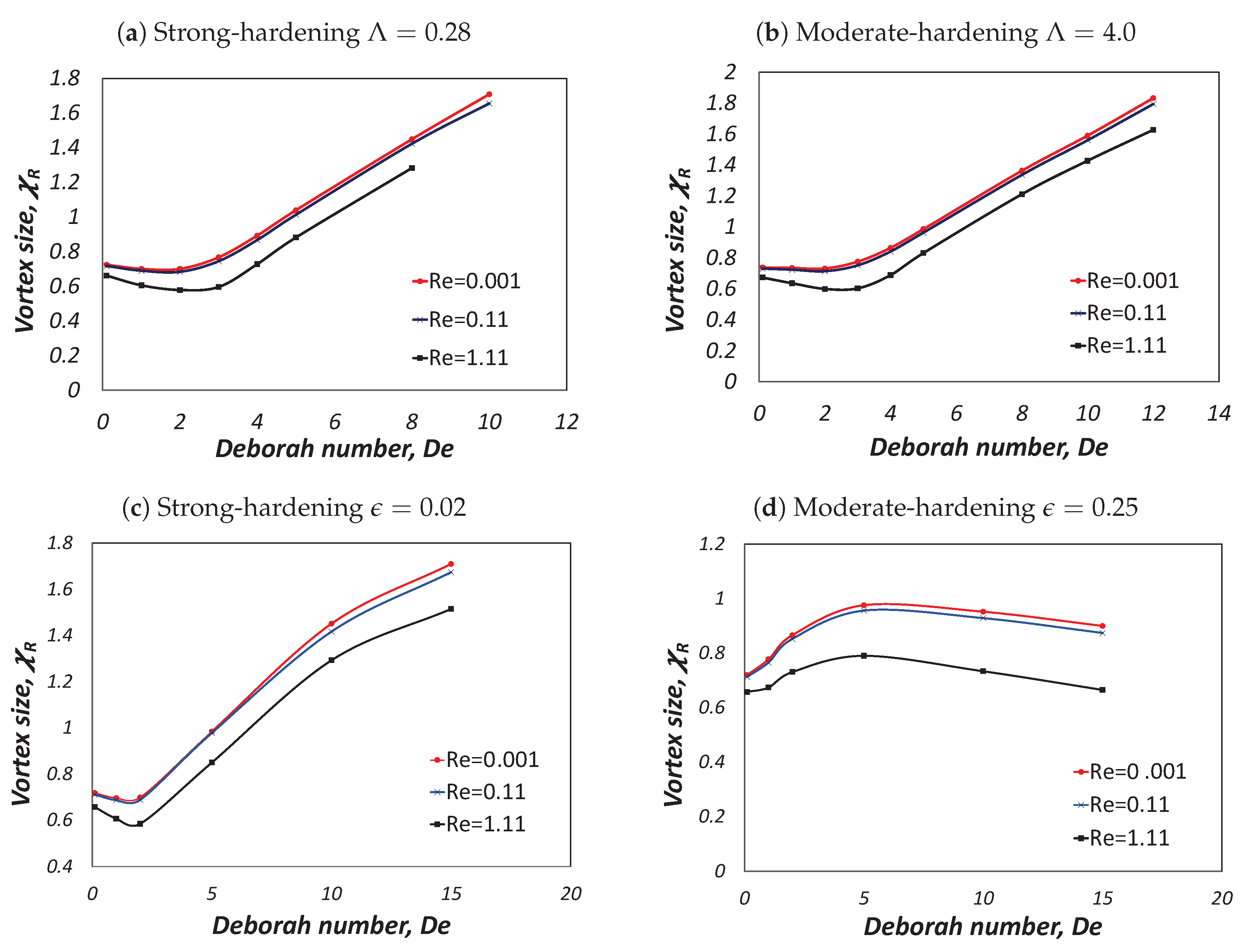
Figure 11.
Transient behavior of the corner vortex size for the planar 4:1 contraction geometry using the MBM model with strong- () (left) and moderate-hardening () (right) thixotropic behaviour for . Inside each figure, from top to bottom, the Reynolds number is being increased.
Figure 11.
Transient behavior of the corner vortex size for the planar 4:1 contraction geometry using the MBM model with strong- () (left) and moderate-hardening () (right) thixotropic behaviour for . Inside each figure, from top to bottom, the Reynolds number is being increased.
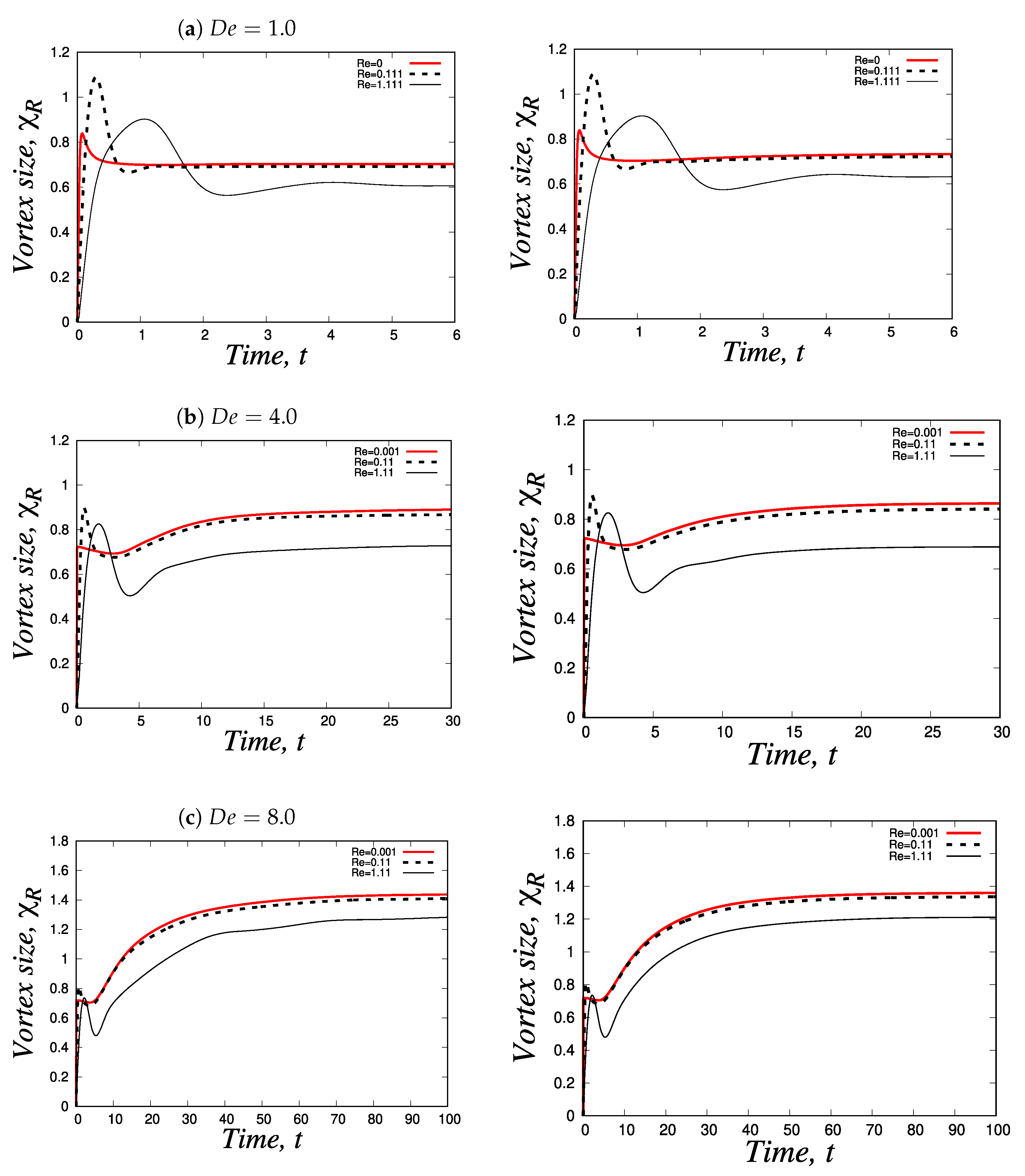
Figure 12.
Transient behavior of the corner vortex size for the planar 4:1 contraction geometry using the MBM model with strong- () hardening behaviour with and .
Figure 12.
Transient behavior of the corner vortex size for the planar 4:1 contraction geometry using the MBM model with strong- () hardening behaviour with and .
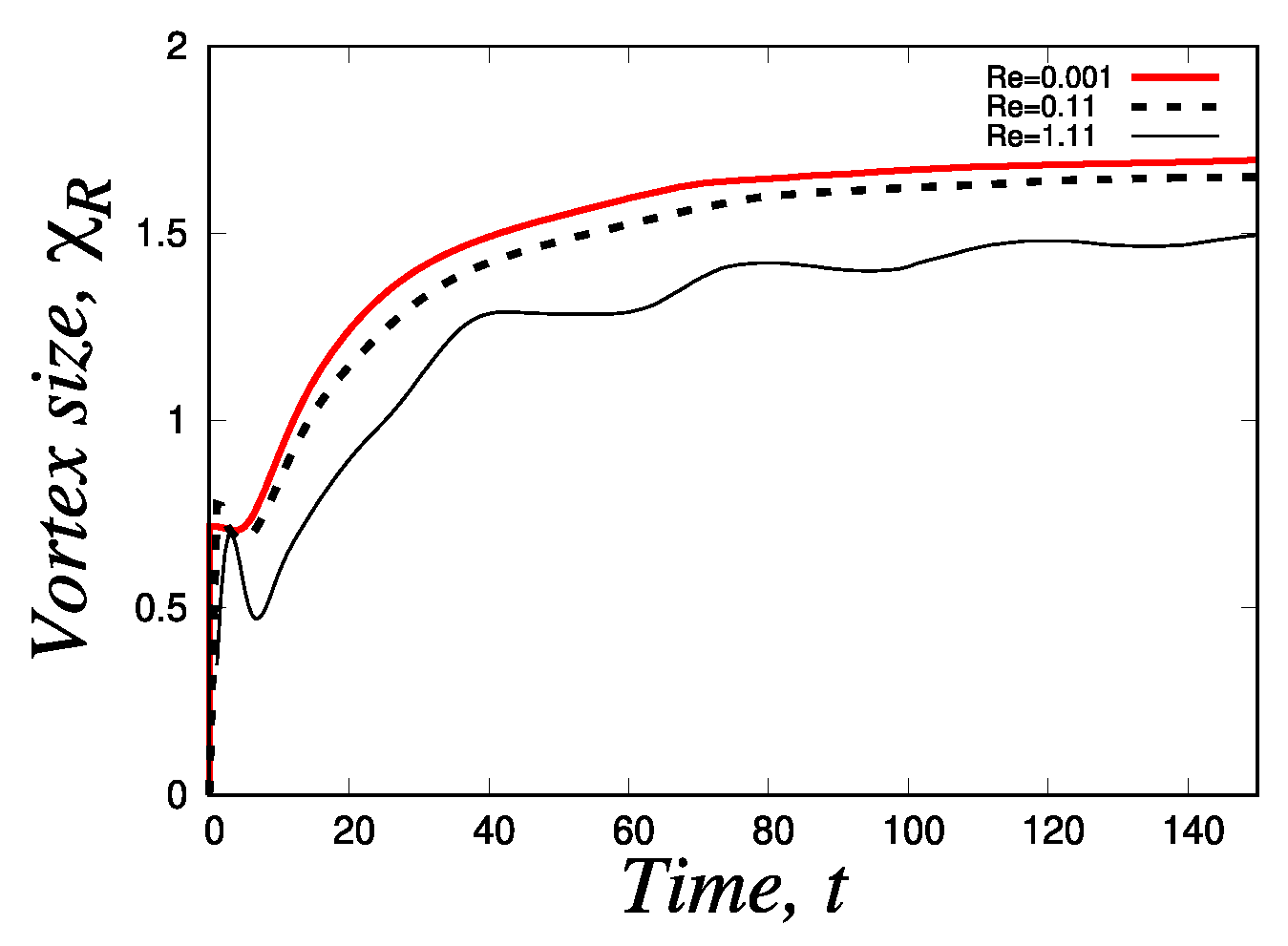
Figure 13.
Fluidity profiles and streamlines obtained from our simulations carried out in the planar contraction 4:1 flow problem using the MBM model for the strong- () and moderate hardening cases () with and fixed. The red line in the streamline figures is a reference line whose length is equal to the highest value of vortex size obtained between the two cases ( for the case ).
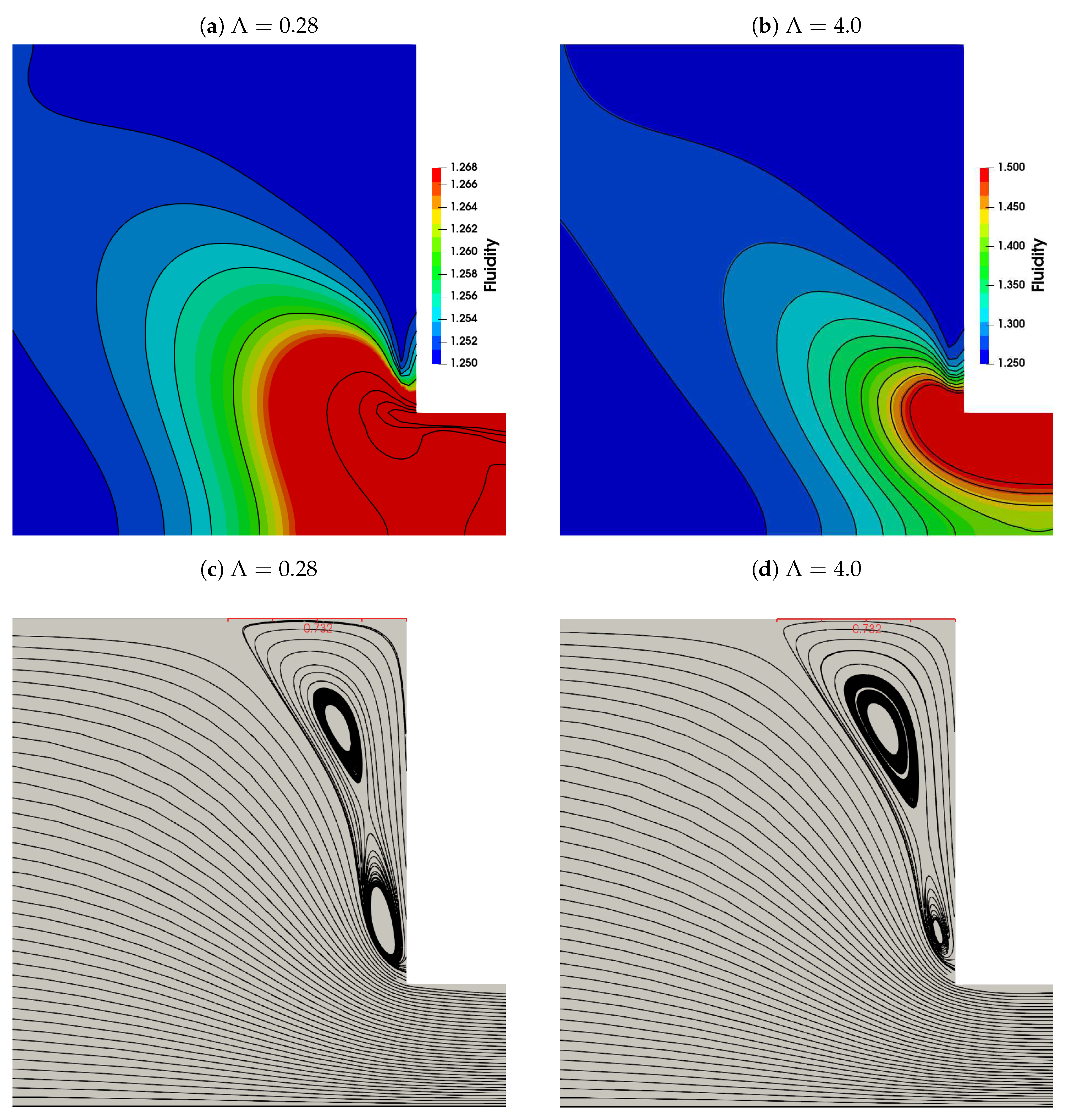
Figure 14.
Fluidity profiles and streamlines obtained from our simulations carried out in the planar contraction 4:1 flow problem using the MBM model for the strong- () and moderate hardening cases () with and fixed. The red line in the streamline figures is a reference line whose length is equal to the highest value of vortex size obtained between the two cases ( for the case ).
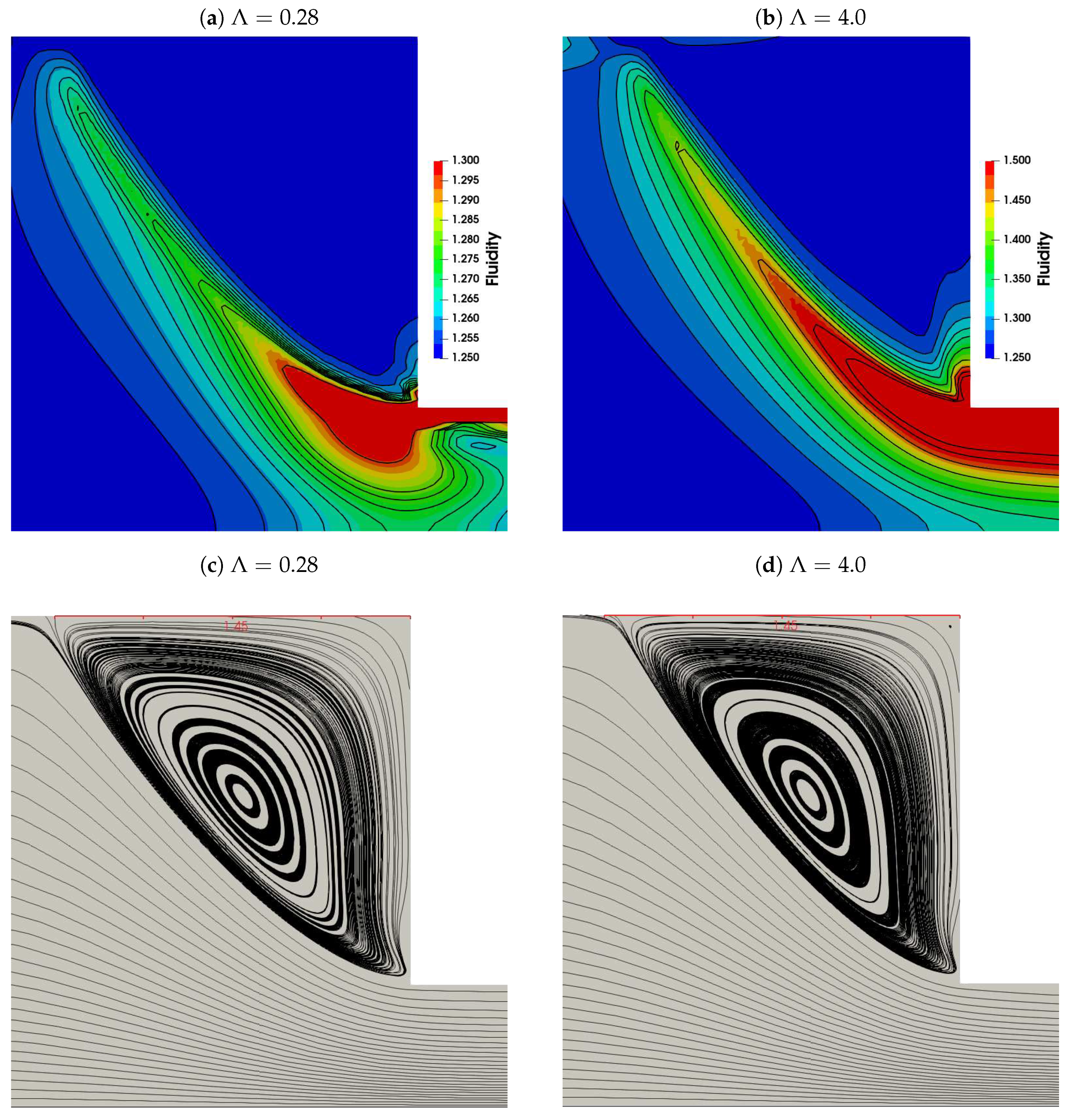
Figure 17.
Transient behavior of the (a) upstream and (b) downstream corner vortexes size for the planar 4:1:4 contraction-expansion geometry using the MBM model for the strong- () (left) and moderate-hardening () (right) thixotropic cases with fixed . In each figure, from top to bottom, the Reynolds number is being increased.
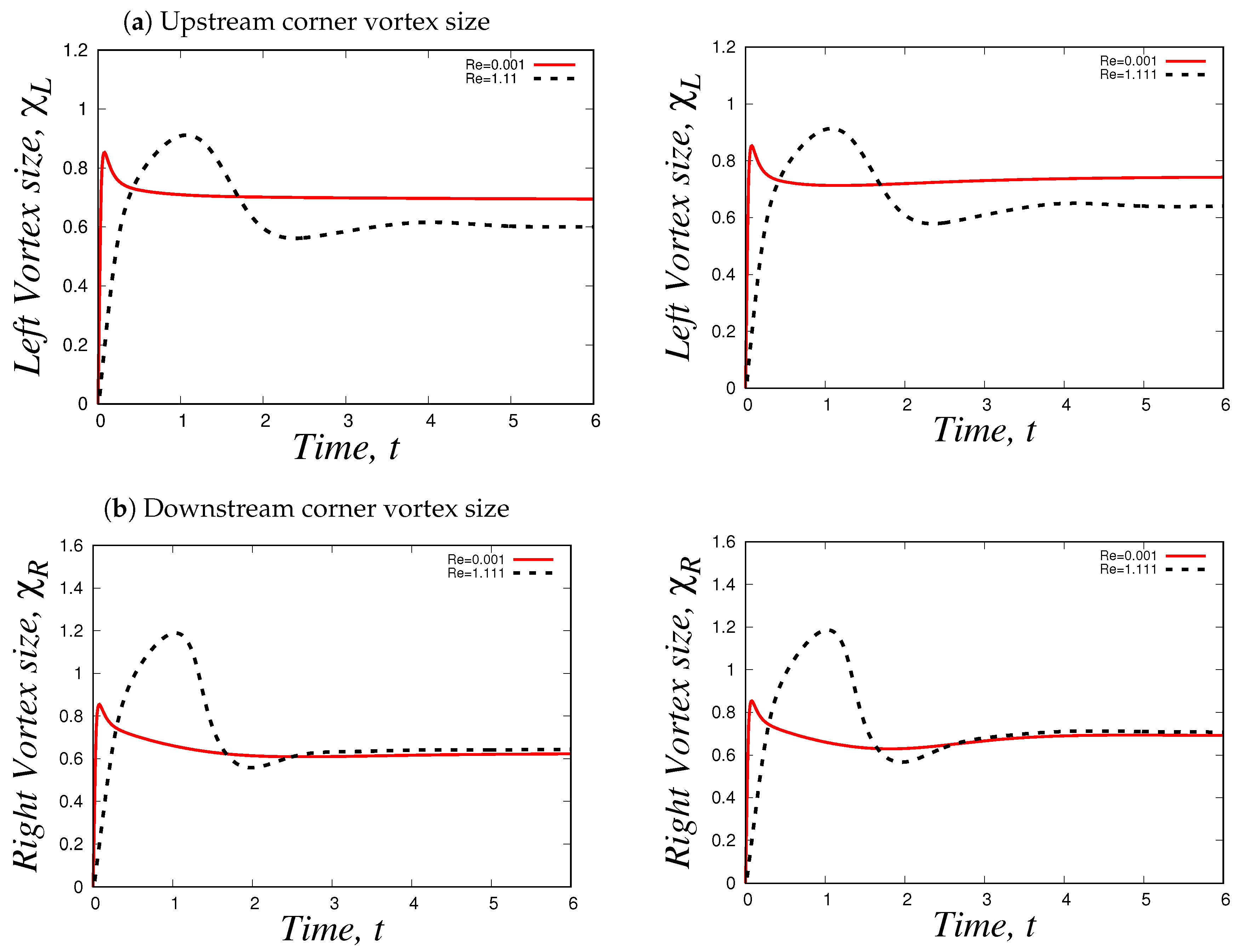
Figure 18.
Streamlines, normalised fluidity and first normal stress difference profiles for the moderate-hardening case () with fixed. The creeping-flow () results are found in the left, while the case is shown in the right.
Figure 18.
Streamlines, normalised fluidity and first normal stress difference profiles for the moderate-hardening case () with fixed. The creeping-flow () results are found in the left, while the case is shown in the right.
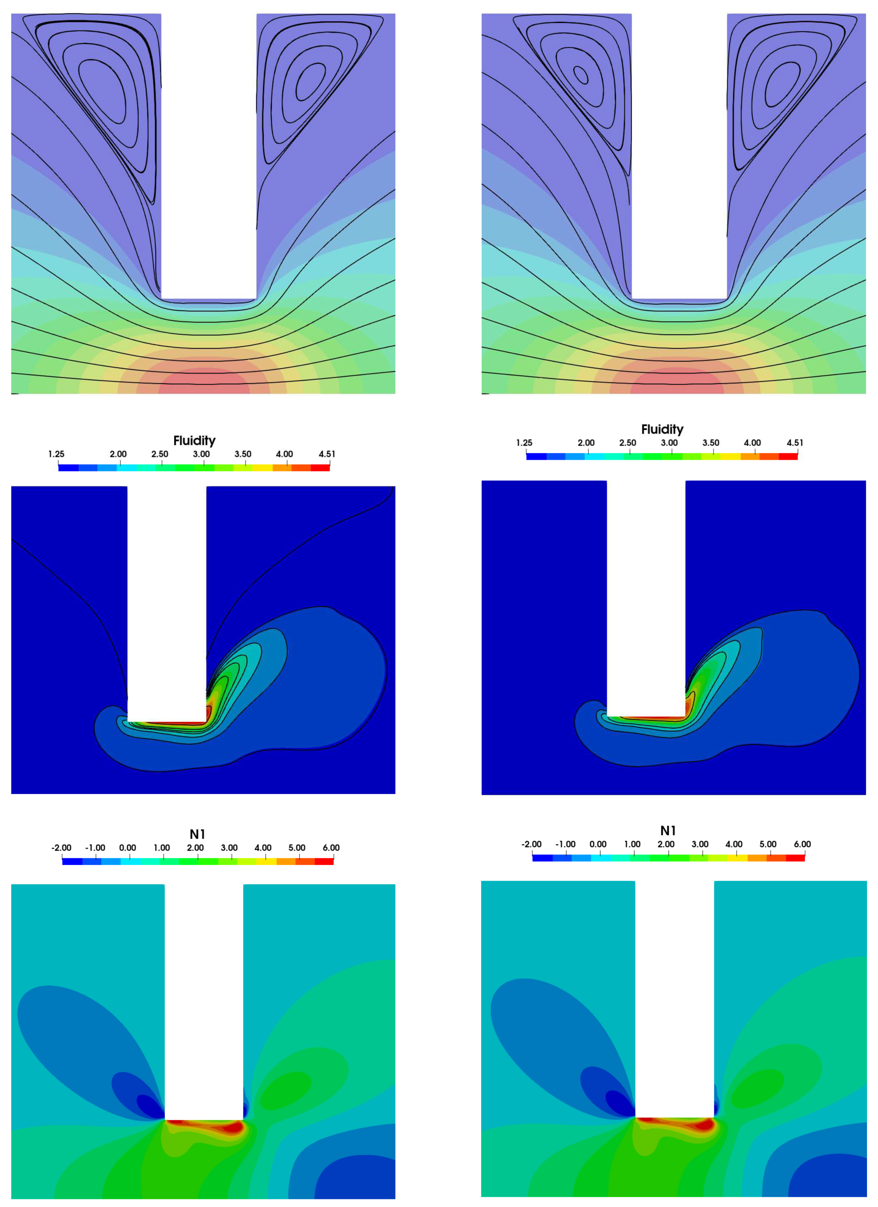
Figure 19.
Streamlines for moderate-hardening case () with fixed. The creeping-flow () results are found in the left, while the case is shown in the right..
Figure 19.
Streamlines for moderate-hardening case () with fixed. The creeping-flow () results are found in the left, while the case is shown in the right..
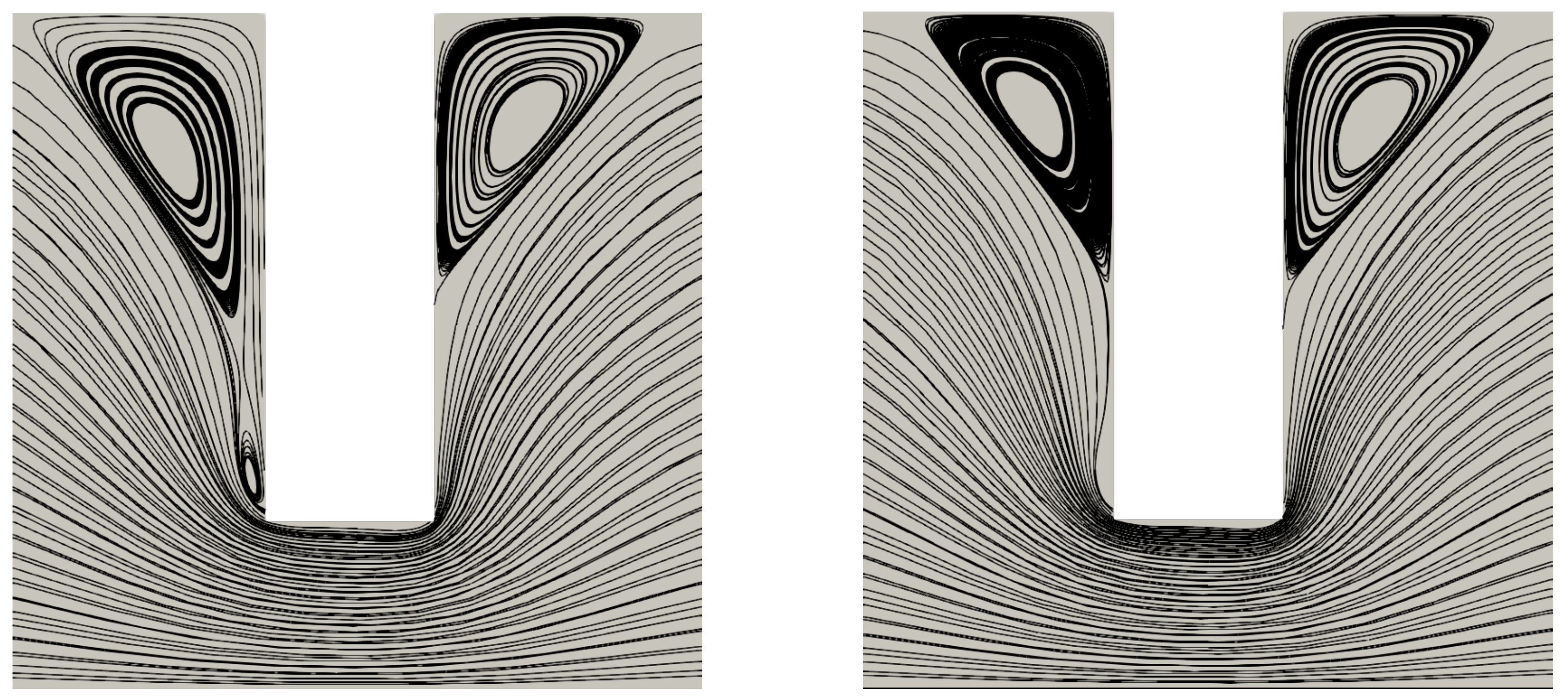
Figure 20.
Streamlines, fluidity and first normal stress difference profiles for the moderate-hardening case () under creeping-flow conditions (). The results for the case are found in the left, while the case is shown in the right. These simulations were carried out without considering the convective term for the fluidity from equation (9).
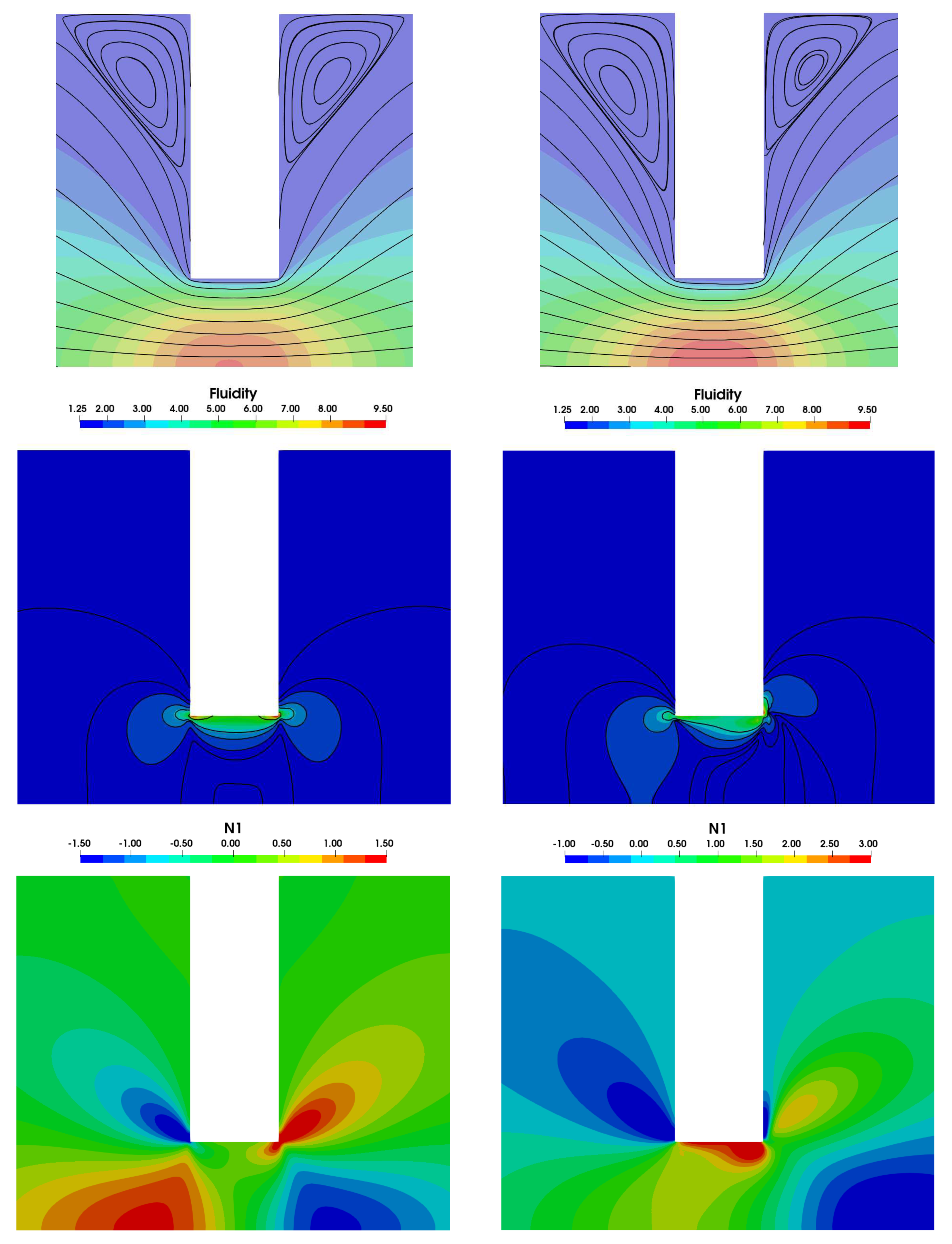

Table 1.
Errors computed for the velocity component in the planar 4:1 contraction flow geometry using the , and norms. The uniform mesh MIII was assumed the reference solution.
Table 1.
Errors computed for the velocity component in the planar 4:1 contraction flow geometry using the , and norms. The uniform mesh MIII was assumed the reference solution.
| Mesh | |||
|---|---|---|---|
| MI | |||
| MII | |||
| RMI | |||
| RMII |
Table 2.
Fixed flow parameter values that will be used to simulate MBM fluids in planar 4:1 contraction and 4:1:4 contraction-expansion geometries.
Table 2.
Fixed flow parameter values that will be used to simulate MBM fluids in planar 4:1 contraction and 4:1:4 contraction-expansion geometries.
| Parameters | Strong-hardening | Moderate hardening |
|---|---|---|
| (m/s) | 1.0 | 1.0 |
| L (m) | 1.0 | 1.0 |
| (s) | 0.28 | 4.0 |
| 0.11 | 0.11 | |
| 0.28 | 4.0 | |
| 0.1125 | 0.1125 |
Table 3.
Steady-state values of the vortex size predicted by the MBM thixotropic model as a function of the Deborah, , the viscoelastic Mach M, the elasticity and the thixoelastic numbers for the strong-hardening case () and for the moderate-hardening case () with , and . The values in brackets and with a star indicate the average value obtained from the range where numerical solutions oscillate.
| Vortex size | M | |||||
|---|---|---|---|---|---|---|
| 0.28 | 0.001 | 0.1 | 0.7243 | 0.0105 | 90.0901 | 0.3571 |
| 1.0 | 0.7009 | 0.0333 | 900.9001 | 3.5714 | ||
| 2.0 | 0.7007 | 0.0471 | 1801.8018 | 7.1428 | ||
| 3.0 | 0.7676 | 0.0577 | 2702.7027 | 10.7143 | ||
| 4.0 | 0.8930 | 0.0666 | 3603.6036 | 14.2857 | ||
| 5.0 | 1.0392 | 0.0745 | 4504.5045 | 17.8571 | ||
| 8.0 | 1.4487 | 0.0942 | 7207.2072 | 28.5714 | ||
| 10.0 | 1.7085 | 0.1054 | 9009.0090 | 35.7143 | ||
| 0.11 | 0.1 | 0.7176 | 0.1053 | 0.9009 | 0.3571 | |
| 1.0 | 0.6902 | 0.3332 | 9.0090 | 3.5714 | ||
| 2.0 | 0.6839 | 0.4712 | 18.0180 | 7.1428 | ||
| 3.0 | 0.7472 | 0.5771 | 27.0270 | 10.7143 | ||
| 4.0 | 0.8673 | 0.6663 | 36.0360 | 14.2857 | ||
| 5.0 | 1.0132 | 0.7450 | 45.0450 | 17.8571 | ||
| 8.0 | 1.4106 | 0.9423 | 72.0720 | 28.5714 | ||
| 10.0 | 1.6553 | 1.0534 | 90.0900 | 35.7143 | ||
| 1.11 | 0.1 | 0.6621 | 0.3333 | 0.0901 | 0.3571 | |
| 1.0 | 0.6060 | 1.0540 | 0.9001 | 3.5714 | ||
| 2.0 | 0.5790 | 1.4906 | 1.8002 | 7.1428 | ||
| 3.0 | 0.5963 | 1.8256 | 2.7003 | 10.7143 | ||
| 4.0 | 0.7281 | 2.1081 | 3.6003 | 14.2857 | ||
| 5.0 | 0.8818 | 2.3569 | 4.5045 | 17.8571 | ||
| 8.0 | 1.2827 | 2.9813 | 7.2007 | 28.5714 | ||
| 10.0 | (1.4871) | 3.3332 | 9.0009 | 35.7143 | ||
| 4.0 | 0.001 | 0.1 | 0.7383 | 0.0105 | 90.0901 | 0.025 |
| 1.0 | 0.7352 | 0.0333 | 900.9009 | 0.25 | ||
| 2.0 | 0.7317 | 0.0471 | 1801.8018 | 0.5 | ||
| 3.0 | 0.7760 | 0.0577 | 2702.7027 | 0.75 | ||
| 4.0 | 0.8650 | 0.0666 | 3603.6036 | 1.0 | ||
| 5.0 | 0.9860 | 0.07450 | 4504.5045 | 1.25 | ||
| 8.0 | 1.3632 | 0.09423 | 7207.2072 | 2.0 | ||
| 10.0 | 1.5899 | 0.1054 | 9009.0090 | 2.5 | ||
| 12.0 | 1.8324 | 0.1154 | 10810.8108 | 3.0 | ||
| 14.0 | 2.0537 | 0.1247 | 12612.61 | 3.5 | ||
| 0.11 | 0.1 | 0.7309 | 0.1054 | 0.9009 | 0.025 | |
| 1.0 | 0.7239 | 0.3317 | 9.0090 | 0.25 | ||
| 2.0 | 0.7142 | 0.4712 | 18.0180 | 0.5 | ||
| 3.0 | 0.7521 | 0.5771 | 27.0270 | 0.75 | ||
| 4.0 | 0.8415 | 0.6663 | 36.0360 | 1.0 | ||
| 5.0 | 0.9634 | 0.7450 | 45.0450 | 1.25 | ||
| 8.0 | 1.3364 | 0.9423 | 72.0720 | 2.0 | ||
| 10.0 | 1.5582 | 1.0536 | 90.0901 | 2.5 | ||
| 12.0 | 1.7812 | 1.1541 | 108.1081 | 3.0 | ||
| 1.11 | 0.1 | 0.6730 | 0.3333 | 0.0901 | 0.025 | |
| 1.0 | 0.6363 | 1.0540 | 0.9001 | 0.25 | ||
| 2.0 | 0.5997 | 1.4906 | 1.8002 | 0.5 | ||
| 3.0 | 0.6033 | 1.8257 | 2.7002 | 0.75 | ||
| 4.0 | 0.6887 | 2.1081 | 3.6004 | 1.0 | ||
| 5.0 | 0.8314 | 2.3569 | 4.5045 | 1.25 | ||
| 8.0 | 1.2116 | 2.9813 | 7.2007 | 2.0 | ||
| 10.0 | 1.4278 | 3.3332 | 9.0009 | 2.5 | ||
| 12.0 | 1.6274 | 3.6513 | 10.8010 | 3.0 |
Table 4.
Steady-state values of the vortex size predicted by the exponential-PTT model as a function of the Deborah, , the viscoelastic Mach M, the elasticity and the ratio numbers for the strong-hardening case () and for the moderate-hardening case () with , and .
Table 4.
Steady-state values of the vortex size predicted by the exponential-PTT model as a function of the Deborah, , the viscoelastic Mach M, the elasticity and the ratio numbers for the strong-hardening case () and for the moderate-hardening case () with , and .
| Vortex size | M | |||||
|---|---|---|---|---|---|---|
| 0.02 | 0.001 | 0.1 | 0.7172 | 0.0105 | 90.0901 | 5.0 |
| 1.0 | 0.6955 | 0.0333 | 900.9009 | 50.0 | ||
| 2.0 | 0.6984 | 0.0471 | 1801.8018 | 100.0 | ||
| 5.0 | 0.9919 | 0.0745 | 4504.5045 | 250.0 | ||
| 10.0 | 1.4520 | 0.1054 | 9009.0090 | 500.0 | ||
| 15.0 | 1.7112 | 0.1290 | 13513.5135 | 750.0 | ||
| 0.11 | 0.1 | 0.7105 | 0.1053 | 0.9009 | 5.0 | |
| 1.0 | 0.6859 | 0.3332 | 9.0090 | 50.0 | ||
| 2.0 | 0.6876 | 0.4712 | 18.0180 | 100.0 | ||
| 5.0 | 0.9777 | 0.7450 | 45.0450 | 250.0 | ||
| 10.0 | 1.4165 | 1.0536 | 90.0900 | 500.0 | ||
| 15.0 | 1.6740 | 1.2903 | 135.1351 | 750.0 | ||
| 1.11 | 0.1 | 0.6558 | 0.3333 | 0.0901 | 5.0 | |
| 1.0 | 0.6063 | 1.0540 | 0.9001 | 50.0 | ||
| 2.0 | 0.5838 | 1.4906 | 1.8002 | 100.0 | ||
| 5.0 | 0.8493 | 2.3569 | 4.5045 | 250.0 | ||
| 10.0 | 1.2921 | 3.3331 | 9.0009 | 500.0 | ||
| 15.0 | 1.5145 | 4.0823 | 13.5014 | 750.0 | ||
| 0.25 | 0.001 | 0.1 | 0.7191 | 0.0105 | 90.0901 | 0.4 |
| 1.0 | 0.7771 | 0.0333 | 900.9009 | 4.0 | ||
| 2.0 | 0.8657 | 0.0471 | 1801.8018 | 8.0 | ||
| 5.0 | 0.9757 | 0.0745 | 4504.5045 | 20.0 | ||
| 10.0 | 0.9517 | 0.1054 | 9009.0090 | 40.0 | ||
| 15.0 | 0.8997 | 0.1290 | 13513.5135 | 60.0 | ||
| 0.11 | 0.1 | 0.7124 | 0.1054 | 0.9009 | 0.4 | |
| 1.0 | 0.7655 | 0.3317 | 9.0090 | 4.0 | ||
| 2.0 | 0.8523 | 0.4712 | 18.0180 | 8.0 | ||
| 5.0 | 0.9560 | 0.7450 | 45.0450 | 20.0 | ||
| 10.0 | 0.9282 | 1.0536 | 90.0900 | 40.0 | ||
| 15.0 | 0.8739 | 1.2903 | 135.1351 | 60.0 | ||
| 1.11 | 0.1 | 0.6574 | 0.3333 | 0.0901 | 0.4 | |
| 1.0 | 0.6736 | 1.0540 | 0.9001 | 4.0 | ||
| 2.0 | 0.7304 | 1.4906 | 1.8002 | 8.0 | ||
| 5.0 | 0.7899 | 2.3569 | 4.5045 | 20.0 | ||
| 10.0 | 0.7332 | 3.3331 | 9.0009 | 40.0 | ||
| 15.0 | 0.6648 | 4.0823 | 13.5014 | 60.0 |
Disclaimer/Publisher’s Note: The statements, opinions and data contained in all publications are solely those of the individual author(s) and contributor(s) and not of MDPI and/or the editor(s). MDPI and/or the editor(s) disclaim responsibility for any injury to people or property resulting from any ideas, methods, instructions or products referred to in the content. |
© 2023 by the authors. Licensee MDPI, Basel, Switzerland. This article is an open access article distributed under the terms and conditions of the Creative Commons Attribution (CC BY) license (http://creativecommons.org/licenses/by/4.0/).
Copyright: This open access article is published under a Creative Commons CC BY 4.0 license, which permit the free download, distribution, and reuse, provided that the author and preprint are cited in any reuse.


