
Submitted:
09 September 2023
Posted:
13 September 2023
You are already at the latest version
Abstract
The vibration response of soil is a key property in the field of agricultural soil tillage. Vibration components of tillage machinery are generally used to reduce tillage resistance and improve work efficiency, the pressure variation under low-frequency vibration will affect the fragmentation and dispersion of farmland soil. However, the gradient of pressure variation, frequency domain response, and effective transmission range are unclear. A new method based on DEM (Discrete Element Method) is presented to study the vibration response and pressure transmission under low-frequency vibration. Bench test results showed that peak pressure positively correlates with the vibration frequency and attenuates rapidly at the vibration distance of 100 to 250 mm. The results data were also selected to determine the simulation model parameters. Amplitude, vibration frequency, and soil depth were used as test factors in single-factor simulation tests, and their effects on the peak pressure, frequency domain response, and effective transmission distance were analyzed. The results showed a positive relationship between the peak pressure and the test factors. The peak pressure increases with a maximum gradient of 19.02 kPa/mm at a vibration distance of 50 mm. The amplitude, vibration frequency, and soil depth positively correlate with the dominant frequency amplitude. The main frequency is independent of amplitude and soil depth. At the vibration distance of 250 mm, the dominant frequency is approximately twice the vibration frequency at 7–11 Hz and approximately equal to the vibration frequency at 13–15 Hz. Multiple exponential functions were used to fit the peak pressure attenuation function, obtaining an effective transmission distance range of 347.15 to 550.37 mm for the 5kPa cut-off pressure. For a soil depth of 300 mm, the vertical shear wave diffusion angle is greater than the horizontal shear wave diffusion angle. The study clarifies the vibration response of soil under low-frequency vibration, which helps to design vibration type soil-engaging components of tillage machinery and match vibration parameters for energy saving and resistance reduction in soil tillage.
Keywords:
soil
; low-frequency
; discrete element method
; vibration response
; transmission
1. Introduction
In recent years, the vibration response of soil has become a research hotspot, due to the energy saving and resistance reduction requirements of agriculture for soil tillage. Agricultural machinery with vibration components (vibration subsoilers, vibrating rotary tillers [1], root crop harvesters with vibrating shovels, etc.) is widely used in soil tillage. The driving torque is provided by the tractor output shaft, and the vibration frequency is generally less than 20 Hz [2,3]. Soil is a complex semi-infinite continuous loose medium whose vibration response is irregular. The mechanical properties (cohesion, elasticity, friction, etc.) of soil will significantly change when excited by the low-frequency vibrations of the components [4]. Therefore, studying the low-frequency vibration response of soil under different vibration conditions is crucial for designing vibration type soil-engaging components of tillage machinery and matching vibration parameters.
With a wide range of pertinent research and applications, the theoretical foundation for the vibration response of continuous rigid bodies is comparatively comprehensive [5,6,7]. Chen et al. [8] developed the excitation parameters of the dynamic model and its vibration response in MATLAB, and the vibration response of the rice combine harvester frame was tested to verify the dynamic model. The irregular contacts between discrete materials particles will lead to large calculating errors. Therefore, a corresponding test analysis is required depending on the material. Pavlovskaia et al. [9] established a vibratory impact drilling system model, analyzed excitation and vibration frequency amplitude as a function of drilling rate, and clarified the optimal loading parameters and strategy. Leonard et al. [10] designed and developed a mechanism that vibrated the soil at a given time, amplitude, and frequency, resulting in compacting the soil and using the vibratory method to determine the maximum bulk density of soils.
The discrete element method is a numerical simulation method used to model discontinuous media. With the ability to obtain data on the forces and movements of particles, it has been introduced into the study of the dynamic behavior of soils [11,12]. Huang et al. [13] proposed a DEM (Discrete Element Method) based method for studying ultrasonic propagation in agricultural soil media and analyzed the influence of excitation parameters on the time-domain and frequency-domain profiles of ultrasonic waves. Qiao et al. [14] investigated the Brazil nut separation under vibration using the discrete element method and predicted both the final segregation degree and the segregation velocity. Amirifar et al. [15] use the discrete element method to present a numerical study on the self-assembly of mono-size granular spheres with periodic boundary conditions under uniform and non-uniform 3D vibration.
Plant roots, farmyard litter, and other materials are frequently found in farmland soils with a media diversity [16], which makes it difficult to collect reliable test results. The advantage of indoor bench tests is that uncertainties can be eliminated, and the test results can be more widely applied. Liu et al. [17] constructed a ballast sensor by embedding a chip and built an impact hammer test rig to analyze the effect of vertical vibration and transmission characteristics of ballast on the dynamic stability of railway track structures. Zhang et al. [18] used a support platform, hammer, and acceleration sensor to build a large cabbage vibration test bench and used stepwise multiple linear regression methods to quantitatively and qualitatively analyze the cabbage quality. In this study, a low-frequency vibration transfer test bench with a parameter (amplitude, vibration frequency, soil depth) adjustment function was constructed. The bench test data are used to obtain response curves between pressure and the vibration frequency and also to verify the accuracy of the soil simulation model. Three sets of single-factor simulation tests were conducted. Peak pressure, frequency domain response, effective transmission distance, and vibration pressure transfer paths are studied to clarify the vibration response. The results can provide an essential reference for designing vibration type soil-engaging components of tillage machinery and matching vibration parameters for energy saving and resistance reduction in soil tillage.
2. Materials and Methods
2.1. Construction of test bench
A low-frequency vibration transfer test bench with amplitude, vibration frequency, and other parameter adjustment functions was constructed, as shown in Figure 1. The test bench consists of a signal generator, a modal vibration exciter, a soil bin, a soil-pressure sensor, a power amplifier, a dynamic signal tester, and a PC. According to the pre-test results, soil bin size is set to 1000 mm (length)×600 mm (width)×600 mm (height). The size of the vibration board of the modal vibration exciter is 50 mm (length)× 40 mm (width)× 5mm (height).
The SA-SG signal generator provides output functions for sine, square, and triangle waveforms, and its sine signal frequency can be adjusted from 2 Hz to 2 kHz. The output waveform frequency is also visible through the LED window. The SA-PA050 power amplifier has a 500 VA rated input power, an AC input frequency response range of 20–50 k±1 dB, and less than 1% high impedance nonlinear distortion. The maximum excitation force, amplitude, and acceleration for the SA-JZ050 modal vibration exciter are 500 N, 10 mm, and 49.5 g, respectively. Receiving signals from the SA-SG signal generator, the modal exciter generates different amplitudes and vibration frequencies. The BWM-28 soil-pressure sensor (BWM, Liyang, China) with a diameter of 28 mm has an accuracy error of 0.1 kPa, a range of 0–100 kPa, and an overload capacity of 120%.
The soil was excavated in the experimental field of Soil-Machine-Plant Key Laboratory (39°.9' N, 116.3' E), which has a north temperate semi-humid continental monsoon climate with an average annual temperature of 9 –19°C and an average annual precipitation of 470 mm to 660 mm. The soil type is cinnamon soil, and the soil particle density measured by the ring knife method is 2600 kg/m3 (The volume of the particles was measured by the drying method and converted to calculate the particle density). After being transported back to the lab, the roots, stones, and farmland garbage were removed from the soil using a circular filter to obtain soil samples with consistent particle sizes. The soil and water quality were weighed separately using the moisture content of the deployment method [19]. After being mixed evenly, covered with film, and left in place for 24 hours (target moisture content 10%). The soil with the adjusted moisture content is poured into the soil bin, pressed down with an iron plate in each 50 mm, filled to the desired volume, and then covered with film and stood for 72 hours. Before the bench test, the soil firmness was measured using a spectrum firmness meter, and a moisture content meter is 1173 kPa and 9.7% moisture content.
2.2. Bench tests of low-frequency vibration
In the previous stage, we worked on the energy-saving and efficient harvesting of root rhizome crops (liquorice, cassava, and potatoes). A lightweight harvester with novel oscillating shovel-rod components was developed, during the harvesting process, the shovel transmits vibration energy in the horizontal direction and breaks up the soil in the vertical direction [20,21,22]. The amplitude, vibration frequency, and soil depth used during the harvesting ranged from 5 to 15 mm, 7 to 15 Hz, and 200 to 400 mm. In this study, the low-frequency (7–15 Hz) are selected to clarify the vibration response, and a single-factor bench test was conducted. The study focuses on the vibration response in the horizontal direction, the soil depth (Hs) is set at 300 mm, and the area of the vibration board is 0.002 m2. Before the test, the soil bin is filled with a soil depth of 400 mm, and the distance between the vibration board and the bottom surface of the soil bin (Hb) is 100 mm (i.e., the soil depth for the bench test is 300 mm). The bottom soil reduces the reflection from the hard substrate. In order to prevent soil leakage from the vibration board action position, a layer of plastic film was placed inside the soil bin in advance.
The internal structure of a modal vibration exciter consists of a magnet exciting coil, a driving coil, a support spring, and a vibration column, which works according to the faraday law of electromagnetic induction, as shown in Figure 2. The power amplifier supplies the driving coil with an electric current of variable frequency, the driving coil is subjected to an electrodynamic force (Fe) proportional to the electric current, calculated by equation (1). The amplitude of the vibration column is non-linearly related to the vibration frequency under the composite action of the elastic and electrodynamic forces. Within a slight vibration frequency variation, the rated amplitude (10 mm) value can be considered constant.
where: B is the mean value of magnetic flux density, T; I is the output electric current value of modal vibration exciter, A; L is the length of the driving coil wire, m.
Pile barriers buried in the soil have a significantly effect on vibration attenuation [23,24]. The soil bin size was small, and only one soil-pressure sensor was buried to eliminate the influence on pressure value measurements (Figure 3). Before the test, the soil in the contact area was compacted to reduce the rebound effect. Burying the soil-pressure sensor could damage the test soil structure. A total of three vibration distances (LV) were tested in the bench test in the sequence of 400, 250, and 100 mm. To minimize the reflection of vibrations from the sidewalls, a paper shell material with a thick honeycomb structure was used.
2.3. Simulation modelling and testing
2.3.1. Simulation modeling and parameters determination
DEM simulation model can ensure the uniform soil conditions among the test groups and extract a wider range of test data. As shown in Figure 4, a 1:1 proportional 3D model of the soil bin, soil-pressure sensor, and vibration board was created using the Inventor 2018 software (Autodesk, San Francisco, USA), saved as .stl file and then imported into the EDEM 2020 software (DEM Solution, Edinburgh, UK) for simulation modeling. In order to apply vibration to soil particles, add sinusoidal translation kinematics to the vibration board in the EDEM 2020 software and make it reciprocate based on the specified amplitude and vibration frequency.
The bonding contact model integrated into the EDEM 2020 software generates virtual cylindrical bonding bonds between particles, which have mechanical properties comparable to those of the finite element method. Referring to the studies [25,26,27] and pretest results, a soil particle radius of 4 mm, a soil density of 2600 kg/m3, a shear modulus of 9.6×10⁶ Pa, and a Poisson ratio of 0.27 were determined. The soil bin's frame and vibration board materials are steel, with a density of 7865 kg/m3, a shear modulus of 7×10⁸ Pa, and a Poisson ratio of 0.35. The internal material of the soil bin with the soil is plastic film, and other parameters are shown in Table 1. The simulation software is EDEM 2020, which operates on a simulation platform with a window 10 64-bit system (CPU: Intel(R) Xeon(R) Gold 6226R, 2.90 GHz, dual CPU, 64 cores; GPU: NVIDIA GeForce RTX 3080), the simulation time step was set to 4.04486×10⁻⁵ s, which is 20% of the Rayleigh time step.
2.3.2. Simulation test
Considering the impact of soil-pressure sensors, only one sensor is buried for each simulation test. The vibration distance was between 0 and 600 mm, with a measurement interval of 50 mm. The simulation test investigated the differences in the low-frequency vibration response of soil for each test factor, setting the sampling frequency to 1000 Hz and the total simulation time to 1 s. Three sets of single-factor simulation tests were run in total, with the other two factors set to 0 levels whenever a single-factor test was performed for a factor (Table 2).
This study aims to obtain the pressure at various vibration distances, analyze the characteristics of its time domain response and frequency domain response, determine the effective transmission distance, describe the soil vibration transfer path, and clarify the low-frequency vibration response of the soil. The indexes and acquisition methods are as follows:
1) Peak pressure (F). In the post-processing interface of EDEM software, the pressure data set of the soil pressure sensor is collected, and the peak pressure is calculated by Equation (2).
where: F is the value of peak pressure, N; FPi is a cycle's maximum pressure value in stable section, N.
2) Frequency domain response. Fourier transforms the time domain signal into the frequency domain signal, applies the findpeak function and plot function of MATLAB 2017 (MathWorks, Massachusetts, USA) software, and plots the peak curve of the frequency domain signal.
3) Effective transmission distance. The scatter data of peak pressure, and vibration distance are taken as input, the peak pressure attenuation function was then fitted using MATLAB 2017 software, and the solve function was used to determine the corresponding distance under the cut-off pressure.
3. Results and discussion
3.1. Analysis of bench test results
Before the test, the soil-pressure sensor was set to 0 kPa, and the signal acquisition frequency of the dynamic signal tester was set to 1000 Hz. The modal vibration exciter was set up with a vibration frequency of 7–15 Hz, an amplitude of 10 mm, and a vibration distance of 250 mm. Each set of tests was performed three times and the test data were averaged. Figure 5a shows the response curve of peak pressure and vibration frequency. Using the vibration parameters of 10 mm amplitude, and 11 Hz vibration frequency, Figure 5b shows the time domain response curve of pressure in each vibration distance.
Peak pressure is positively correlated with vibration frequency and negatively correlated with vibration distance (Figure 5a). The peak pressure increases by 4.66, 1.55, and 0.74 kPa/mm at vibration distances of 100, 250, and 400 mm, respectively. Different vibration distances have the same response cycle for the peak pressure (Figure 5b), and the "sine-like" vibration waveform may be related to the viscoelastic plasticity of the soil. The pressure rises rapidly during the loading stage, reaches a transient peak, and forms a small wave during the unloading stage. In low-stiffness materials, the vibration energy attenuates rapidly [28,29]. The pressure attenuation gradient is approximately 0.34 kPa/mm when the vibration distance is less than 250 mm. The vibration pressure is small in the range of 250 mm to 400 mm, and the attenuation gradient is approximately 0.099 kPa/mm.
3.2. Analysis of simulation model accuracy
After determining the contact parameters for the soil particles, a set of comparative tests were carried out to verify the accuracy of the simulation model. The bench test was carried out to choose the vibration frequency of 9, 11, and 13 Hz, and the target values were the peak pressures at vibration distances of 100, 250, and 400 mm. As shown in Figure 6, the relative errors between the simulated and measured values are less than 8.64%, 10.03%, and 10.22% for the source distance of 100mm, 250mm, and 400mm, respectively, at each vibration frequency. The peak pressure at the vibration distance of 250mm and 400mm is small, and relatively small differences will produce large relative errors. The simulation results are generally consistent with the measured results, showing that the discrete element method can be used to simulate the low-frequency vibration response of the soil.
3.3. Analysis of simulation test results
3.3.1. Peak pressure
The response curve in Figure 7a shows that the peak pressure at each vibration distance gradually increases as the amplitude increases, which may cause as the amplitude increases, the applied energy gradually increases, and the soil particle movement is more active, resulting in a gradual increase in the impact force on the pressure sensor. The largest increase gradient in peak pressure is 19.02 kPa/mm, measured at a vibration distance of 50 mm. The extreme difference in peak pressure at a vibration distance of 450 mm is 4.41 kPa, which is slightly influenced by the change in amplitude.
The response curve in Figure 7b shows that the peak pressure at each vibration distance gradually increases as the vibration frequency increases, which is consistent with the bench test results. Increased vibration frequency causes the impact on the soil particles more frequently. The soil may obtain more elastic energy, the particles shake violently, and the peak pressure gradually increases. The largest increase gradient in peak pressure is 9.38 kPa/Hz, measured at a vibration distance of 50 mm. The extreme difference at a vibration distance of 400 mm is 5.12 kPa. When the vibration distance exceeds 400 mm, the effect of changes in vibration frequency is slight.
The peak pressure at each vibration distance gradually increases as the soil depth increases, according to the response curve in Figure 7c. As soil depth increases, the discrete nature of the soil medium decreases, and transmit pressure ability of soil particles increases, resulting in a gradual increase in peak pressure. The largest increase gradient of the peak pressure is 0.45 kPa/mm, at a vibration distance of 50 mm. The extreme difference in the peak pressure at the vibration source of 450 mm is 4.42 kPa. The variation in soil depth slightly influences the peak pressure when the vibration distance is above 450 mm.
3.3.2. Frequency domain response
In the response of a nonlinear system, the primary resonances are the excitation frequency close to the natural frequency and the sub-harmonic resonance close to an integer multiple of the natural frequency [30]. Agree with its point of view, the frequency domain signal of the soil is very complex after being vibrated. The frequency domain signal at the vibration distance of 250 mm was processed using MATLAB 2017 software, with the minimum peak prominence of the findpeaks function set to 0.08, to visually compare and analyze the differences in the components of the frequency domain signal, as shown in Figure 8. The y-coordinate of frequency domain signal is magnitude, from which the main frequency and main frequency amplitude are extracted, as shown in Table 3, Table 4 and Table 5.
In the frequency range from 0 to 50 Hz, the frequency multiplication and frequency division signal values are positively correlated with the amplitude, as shown in Figure 8a. The dominant frequency amplitude has increased gradients of 0.16/mm and 1.14/mm for the amplitude of 10 mm and 12.5 mm, respectively, which are minimum and maximum values. The dominant frequency is approximately twice the vibration frequency, as shown in Table 3. The dominant frequency amplitude gradually increases with the amplitude, reaching a maximum value (11.99 kPa) at 15 mm. When the vibration frequency is 11 Hz, the dominant frequency is relevant to the elastic hysteresis of soil (the elastic deformation takes some time to return to its normal value after loading or unloading), which causes the soil to be positively vibrated by the vibration board during the rebound cycle, resulting in the dominant frequency being approximate twice the vibration frequency. When the amplitude is in the range of 5 to 15 mm, increasing the amplitude only improves the pressure, and the frequency response of the soil is unaffected.
In the frequency range from 0 to 100 Hz, the frequency multiplication and frequency division signal values are positively correlated with the vibration frequency, as shown in Figure 8b. The dominant frequency amplitude has increased gradients of 0.27/Hz and 1.77/Hz for vibration frequency of 9 Hz and 13 Hz, respectively, which are minimum and maximum values. The dominant frequency is approximately twice the vibration frequency at 7–11 Hz and approximately equal to the vibration frequency at 13–15 Hz, as shown in Table 4. The dominant frequency amplitude reaches the maximum (12.03 kPa) at 15 Hz. The vibration impact response time between soil particles is shortened at a vibration frequency greater than 13 Hz, potentially eliminating vibration hysteresis. When the vibration frequency is between 13 and 15 Hz, increasing the vibration frequency will enhance the pressure and change the frequency response of the soil.
In the frequency range from 0 to 50 Hz, the frequency multiplication and frequency division signal values positively correlate with the soil depth, as shown in Figure 8c. The amplitude difference between the frequency multiplication and frequency division signal is minimal at a frequency greater than 50 Hz. As the soil depth increases, the least increasing gradient (0.011/mm) of the dominant frequency at a soil depth of 250 mm and the most (0.0314/mm) at 350 mm. The dominant frequency amplitude gradually increases with increasing soil depth, reaching a maximum value (10.41 kPa) at 400 mm, as shown in Table 5. The dominant frequency of the soil is approximately twice that vibration frequency at various soil depths. As soil depth increases, the soil's ability to store and transmit pressure increases with depth while the frequency response rule remains constant.
By analyzing the result data, the generation of the dominant vibration frequency may be affected by the soil's viscoelastic plasticity, and the dominant frequency's magnitude is obtained as 1/2 of the applied vibration frequency. The frequency domain component of 300 ~ 400 Hz may be related to the reflection effect of the soil bin on the vibration.
3.3.3. Effective transmission distance
The vibration applied to the soils will change the physical characteristics, such as porosity, cohesion, and elastoplastic. The effective transmission distance is one of the most important indexes for studying the vibration response of soil. An accurate attenuation model can characterize soil vibration propagation and attenuation characteristics [31,32,33]. The vibration distance LV was used as the independent variable, the peak pressure F as the dependent variable, and the MATLAB 2017 software was used to model the peak pressure attenuation function. The effective transmission distance of pressure is determined by solving the function. The confidence R2 values of the multiple exponential function fitting methods were greater than 0.9874, which can accurately characterize the attenuation of peak pressure. When the peak pressure is less than 5 kPa, it decreases very slowly with increasing vibration distance, as shown in Figure 9. So, the cut-off pressure is selected at 5 kPa.
When the amplitude increases, the coefficient of the peak pressure attenuation function gradually increases, and the variation gradient of pressure increases (Figure 10a). At amplitude of 5 mm and 15 mm, minimum and maximum peak pressures of 320 kPa and 1610 kPa were obtained at the vibration board-soil interface, respectively. The effective transmission distance of the pressure to the low-frequency vibration is 416.25, 444.45, 465.73, 512.48, and 555.37 mm for each amplitude (5, 7.5, 10, 12.5, and 15 mm). The attenuation gradient of pressure increases slightly as the vibration frequency increases, as shown in Figure 10b. At vibration frequencies of 7 Hz and 15 Hz, minimum and maximum peak pressures of 200 kPa and 520 kPa were obtained at the vibration board-soil interface, respectively. The effective transmission distance is calculated by putting the cut-off pressure into the function for each vibration frequency (7, 9, 11, 13, and 15 Hz). These values are 347.15, 424.31, 465.73, 502.48, and 550.21 mm, respectively. As the soil depth increases, the peak pressure decreases, and the coefficient of the peak pressure attenuation function gradually increases (Figure 10c). At soil depths of 200 mm and 400 mm, minimum and maximum peak pressures of 155 kPa and 450 kPa were obtained at the vibration board-soil interface, respectively. For each soil depth (200, 250, 300, 350, and 400 mm), the cut-off pressure was calculated to be 370.81, 422.88, 465.73, 487.97, and 531.58 mm, respectively
3.3.4. Vibration pressure transfer path
Obtaining the forces and movements of the soil particles is helpful for clarifying the vibration pressure transfer paths. A test group with the vibration parameters of 10 mm amplitude, 11 Hz vibration frequency, 300 mm soil depth, and 100 mm vibration distance was selected for the simulation analysis. The soil particle properties were set to vector in the post-processing interface of the EDEM 2020 software, and the clipping command was used to obtain a front and vertical view of the soil bin, as shown in Figure 11.
After being vibrated by low-frequency vibration, pressures are transmitted in the soil as waveforms [34], forming compressional and shear waves on the free surface of the soil. During the pre-loading stage, the soil particles in the contact area tend to move diagonally downwards (points a to point b), as shown in the front view. These particles are under pressure and produce large velocities and displacements, while the soil particles outside the contact area only slightly change. The vibration board compresses soil particles during the loading stage (points b to c). The soil particles in the contact area obtain a larger force and displacement, and the direction of movement changes. At the further end, the force on soil particles increases, but the displacement and direction of movement change slightly. The possible reason is that the pressure increases by compression and the movement of the vibration board is converted into the compression displacement of the soil. The red color of the soil particles in the lower half of the vibration board is more concentrated, indicating that its pressure is greater than the soil above. The shear wave diffusion angle in the vertical direction is approximately 103° and is measured by the angle between the two black dashed lines at point c. The soil particles suffer internal force during pre-unloading (points c to d), and internal elastoplastic pushes them back toward their original position.
From the vertical view, soil particles in the pre-loading stage (points a' to b') are subjected to increased forces in the contact area, and the movement is ordered. The vibration board presses the soil particles in the loading stage (points b' to c'), and the forces on both sides of the vibration board axis are uniform. The soil is vibrated, and the pressure diffuses to both sides. The angle between the two black dashed lines at point c' is the horizontal diffusion angle of the shear wave, which is approximately 85°. The soil particles suffer internal force during the pre-unloading stage (points c' to d') and move back toward the original position.
4. Conclusion
In this study, a low-frequency vibration transfer test bench was constructed, and a single-factor bench test was conducted. The bench test results were analyzed to obtain pressure response curves and used to determine the simulation model parameters. In addition, the influence of the test factors on the peak pressure, frequency domain response, and effective transmission distance is analyzed by simulation tests, while the vibration pressure transfer path of the soil is discussed.
(1) The peak pressure positively correlates with the amplitude, vibration frequency, and soil depth. The pressure attenuates rapidly at a vibration distance of 0 to 250 mm. When the vibration distance is greater than 500 mm, the pressure is slightly affected by the parameters.
(2) The dominant frequency amplitude positively correlates with the amplitude, vibration frequency, and soil depth. The main frequency is independent of amplitude and soil depth. At the vibration distance of 250 mm, the dominant frequency is approximately twice the vibration frequency at 7–11 Hz and approximately equal to the vibration frequency at 13–15 Hz.
(3) Multiple exponential functions can be used to accurately fit the peak pressure attenuation curve. For a cut-off pressure of 5 kPa, the effective transmission distance ranges between 347.15 and 550.37 mm. Beyond the effective transmission distance, the gradient of pressure variations in the soil is slight, but the pressure signal extends over a long distance.
(4) Pressure is transmitted by forward diffusion. In the loading stage, the soil particles outside the contact area are subjected to increased forces, but slight changes in movement. When the soil depth is 300 mm, the shear wave diffusion angle in the vertical direction is greater than that in the horizontal direction.
We tested the vibration response of soil under low-frequency vibration by soil bin test and described the vibration pressure transfer path in the effective distance, which is of great academic value in soil tillage study. In future research, the influence of vibration transmission by the boundary reflection of the test device, the influence of soil moisture content on the test results, and the applicability of field and in-situ tests will be discussed.
Author Contributions
Conceptualization, Methodology, Formal analysis, Writing—original draft, Writing—review & editing, Lipengcheng Wan; Software, Supervision, Project administration, Yonglei Li; Writing—original draft, Supervision, Jinyu Song; Writing—review & editing, Supervision, Xiang Ma; Visualization, Supervision, Xiangqian Dong; Writing—original draft, Supervision, Chao Zhang; Project administration, Supervision, Jiannong Song.
Funding
This work was supported by the National Key Research and Development Program of China (2022YFD2002005).
Institutional Review Board Statement
Not applicable.
Data Availability Statement
Not applicable.
Conflicts of Interest
The authors declare no conflict of interest.
References
- Xiao, M., Niu, Y., Wang, K., Zhu, Y., Zhou, J., Ma, R. Design of Self-excited Vibrating Rotary Tiller and Analysis of Its Performance in Reducing Torsion and Consumption. Nongye Jixie Xuebao/Transactions Chinese Soc. Agric. Mach. 2022, 53, 52–63. [CrossRef]
- Awuah, E., Zhou, J., Liang, Z., Aikins, K.A., Gbenontin, B.V., Mecha, P., Makange, N.R. Parametric analysis and numerical optimisation of Jerusalem artichoke vibrating digging shovel using discrete element method. Soil Tillage Res. 2022, 219, 105344. [CrossRef]
- Wang, Y., Zhang, D., Yang, L., Cui, T., Jing, H., Zhong, X. Modeling the interaction of soil and a vibrating subsoiler using the discrete element method. Comput. Electron. Agric. 2020, 174. [CrossRef]
- Liu, Guoyang, Xia, J., Zheng, K., Cheng, J., Wang, K., Zeng, R., Wang, H., Liu, Z. Effects of vibration parameters on the interfacial adhesion system between soil and metal surface. Soil Tillage Res. 2022, 218. [CrossRef]
- Ding, H., Kaup, A., Wang, J.T., Lu, L.Q., Altay, O. Real-time hybrid simulation framework for the investigation of soil-structure interaction effects on the vibration control performance of shape memory alloys. Eng. Struct. 2021, 243, 112621. [CrossRef]
- Huang, X., Zeng, Z., Li, Z., Luo, X., Yin, H., Wang, W. Experimental study on vibration characteristics of the floating slab with under-slab polyurethane mats considering fatigue loading effect. Eng. Struct. 2023, 276, 115322. 2023; 276, 115322. [CrossRef]
- Zhu, C., Yang, J. Vibration transmission and energy flow analysis of variable stiffness laminated composite plates. Thin-Walled Struct. 2022, 180, 109927. [CrossRef]
- Chen, S., Zhou, Y., Tang, Z., Lu, S. Modal vibration response of rice combine harvester frame under multi-source excitation. Biosyst. Eng. 2020, 194, 177–195. [CrossRef]
- Pavlovskaia, E., Hendry, D.C., Wiercigroch, M. Modelling of high frequency vibro-impact drilling. Int. J. Mech. Sci. 2015, 91, 110–119. [CrossRef]
- Leonard, L., Ekwue, E.I., Taylor, A., Birch, R. Evaluation of a machine to determine maximum bulk density of soils using the vibratory method. Biosyst. Eng. 2019, 178, 109–117. [CrossRef]
- Jia, Y., Zhang, J., Chen, X., Miao, C., Zheng, Y. Computers and Geotechnics DEM study on shear behavior of geogrid-soil interfaces subjected to shear in different directions. Comput. Geotech. 2023, 156, 105302. [CrossRef]
- Kim, Y.S., Siddique, M.A.A., Kim, W.S., Kim, Y.J., Lee, S.D., Lee, D.K., Hwang, S.J., Nam, J.S., Park, S.U., Lim, R.G. DEM simulation for draft force prediction of moldboard plow according to the tillage depth in cohesive soil. Comput. Electron. Agric. 2021, 189, 106368. 2021; 189, 106368. [CrossRef]
- Huang, S., Lu, C., Li, H., He, J., Wang, Q., Yuan, P., Gao, Z., Wang, Y. Transmission rules of ultrasonic at the contact interface between soil medium in farmland and ultrasonic excitation transducer. Comput. Electron. Agric. 2021, 190, 106477. [CrossRef]
- Qiao, J., Duan, C., Dong, K., Wang, W., Jiang, H., Zhu, H., Zhao, Y. DEM study of segregation degree and velocity of binary granular mixtures subject to vibration. Powder Technol. 2021, 382, 107–117. [CrossRef]
- Amirifar, R., Dong, K., Zeng, Q., An, X., Yu, A. Effect of vibration mode on self-assembly of granular spheres under three-dimensional vibration. Powder Technol. 2021, 380, 47–58. [CrossRef]
- Jones, S., Hunt, H. Predicting surface vibration from underground railways through inhomogeneous soil. J. Sound Vib. 2012, 331, 2055–2069. [CrossRef]
- Liu, Ganzhong, Cong, J., Wang, P., Du, S., Wang, L., Chen, R. Study on vertical vibration and transmission characteristics of railway ballast using impact hammer test. Constr. Build. Mater. 2022, 316, 125898. [CrossRef]
- Zhang, J., Wang, J., Zheng, C., Guo, H., Shan, F. Nondestructive evaluation of Chinese cabbage quality using mechanical vibration response. Comput. Electron. Agric. 2021, 188, 106317. [CrossRef]
- Jiang, L., Dongxing, Z., Li, Y., Tao, C., Xiantao, H., Tiancheng, Y. The research of using common probe sensors on dynamic soil moisture content measurement during furrow opening. Meas. J. Int. Meas. Confed. 2022, 192, 110825. [CrossRef]
- Wan Lipengcheng, L.Y., Zhao Hu, Xu Guanghao, Song Jiannong, Dong Xiangqian, Zhang Chao, W.J. Gradient throwing characteristics of oscillating slat shovel for rhizome crop harvesters. Trans. Chinese Soc. Agric. Eng. 2021, 37, 9–21. http://zgnydxxb. ijournals.cn/zgnydxxb/ch/reader/view_abstract.aspx?file_no=20211219&flag=1.
- Wan, L., Li, Y., Zhang, C., Ma, X., Song, J., Dong, X., Wang, J. Performance Evaluation of Liquorice Harvester with Novel Oscillating Shovel-Rod Components Using the Discrete Element Method. Agric. 2022, 12. [CrossRef]
- Wan Lipengcheng, Li Yonglei, Huang Jinqiu, Song Jiannong, Dong Xiangqian, W.J. Driving Torque Characteristics of Oscillating Slat Shovel for Rhizome Crops Harvest Device. Trans. Chinese Soc. Agric. Mach. 2022, 53, 191–200. http://www.j-csam.org/jcsam/ch/reader/view_abstract.aspx?flag=1&file_no=2022s120&journal_id=jcsam.
- Álamo, G.M., Bordón, J.D.R., Aznárez, J.J., Lombaert, G. The effectiveness of a pile barrier for vibration transmission in a soil stratum over a rigid bedrock. Comput. Geotech. 2019, 110, 274–286. [CrossRef]
- Meng, L., Cheng, Z., Shi, Z. Vibration mitigation in saturated soil by periodic pile barriers. Comput. Geotech. 2020, 117, 103251. [CrossRef]
- Shaikh, S.A., Li, Y., Ma, Z., Chandio, F.A., Tunio, M.H., Liang, Z., Solangi, K.A. Discrete element method (DEM) simulation of single grouser shoe-soil interaction at varied moisture contents. Comput. Electron. Agric. 2021, 191, 106538. [CrossRef]
- Tekeste, M.Z., Way, T.R., Syed, Z., Schafer, R.L. Modeling soil-bulldozer blade interaction using the discrete element method (DEM). J. Terramechanics. 2020, 88, 41–52. [CrossRef]
- François, S., Schevenels, M., Thyssen, B., Borgions, J., Degrande, G. Design and efficiency of a composite vibration isolating screen in soil. Soil Dyn. Earthq. Eng. 2012, 39, 113–127. [CrossRef]
- Katinas, E., Chotěborský, R., Linda, M., Jankauskas, V. Wear modelling of soil ripper tine in sand and sandy clay by discrete element method. Biosyst. Eng. 2019, 188, 305–19. [CrossRef]
- Van hoorickx, C., Schevenels, M., Lombaert, G. Double wall barriers for the reduction of ground vibration transmission. Soil Dyn. Earthq. Eng. 2017, 97, 1–13. [CrossRef]
- Zhou, J., Xu, L., Zhang, A., Hang, X. Finite element explicit dynamics simulation of motion and shedding of jujube fruits under forced vibration. Comput. Electron. Agric. 2022, 198, 107009. [CrossRef]
- Ren, X., Wu, J., Tang, Y., Yang, J. Propagation and attenuation characteristics of the vibration in soft soil foundations induced by high-speed trains. Soil Dyn. Earthq. Eng. 2019, 117, 374–383. [CrossRef]
- Auersch, L. Train-induced ground vibration due to the irregularities of the soil. Trans. Chinese Soc. Agric. Mach. 2021, 140, 106438. [Google Scholar] [CrossRef]
- Auersch, L. Mitigation of railway induced vibration at the track, in the transmission path through the soil and at the building. Procedia Eng. 2017, 199, 2312–2317. [Google Scholar] [CrossRef]
- Dutta, T.T., Otsubo, M., Kuwano, R. Stress wave transmission and frequency-domain responses of gap-graded cohesionless soils. Soils Found. 2021, 61, 857–873. [CrossRef]
Figure 1.
Composition of low-frequency vibration transmission test bench.
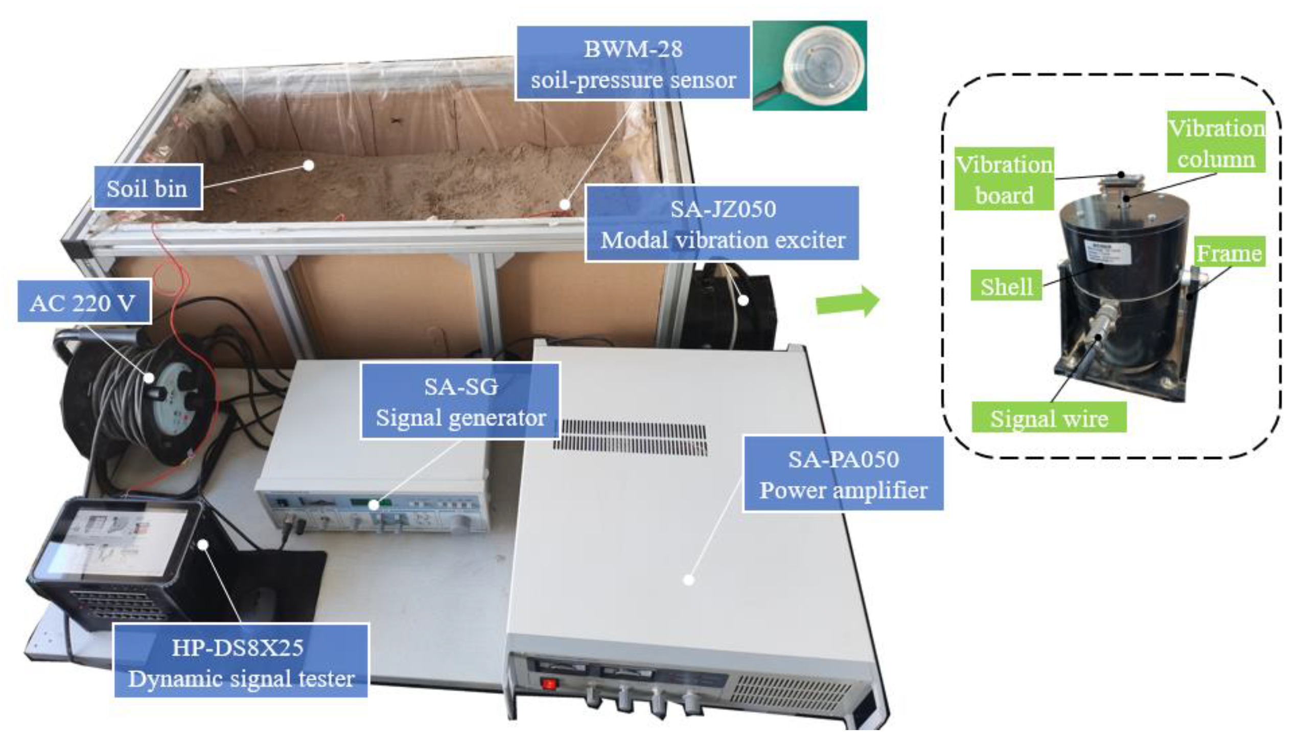
Figure 2.
Internal structure of the modal vibration exciter.
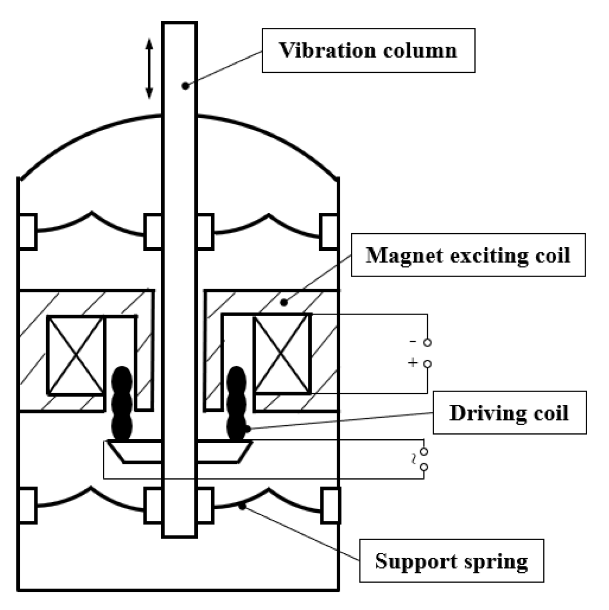
Figure 3.
Diagram of low–frequency vibration transfer in soil.
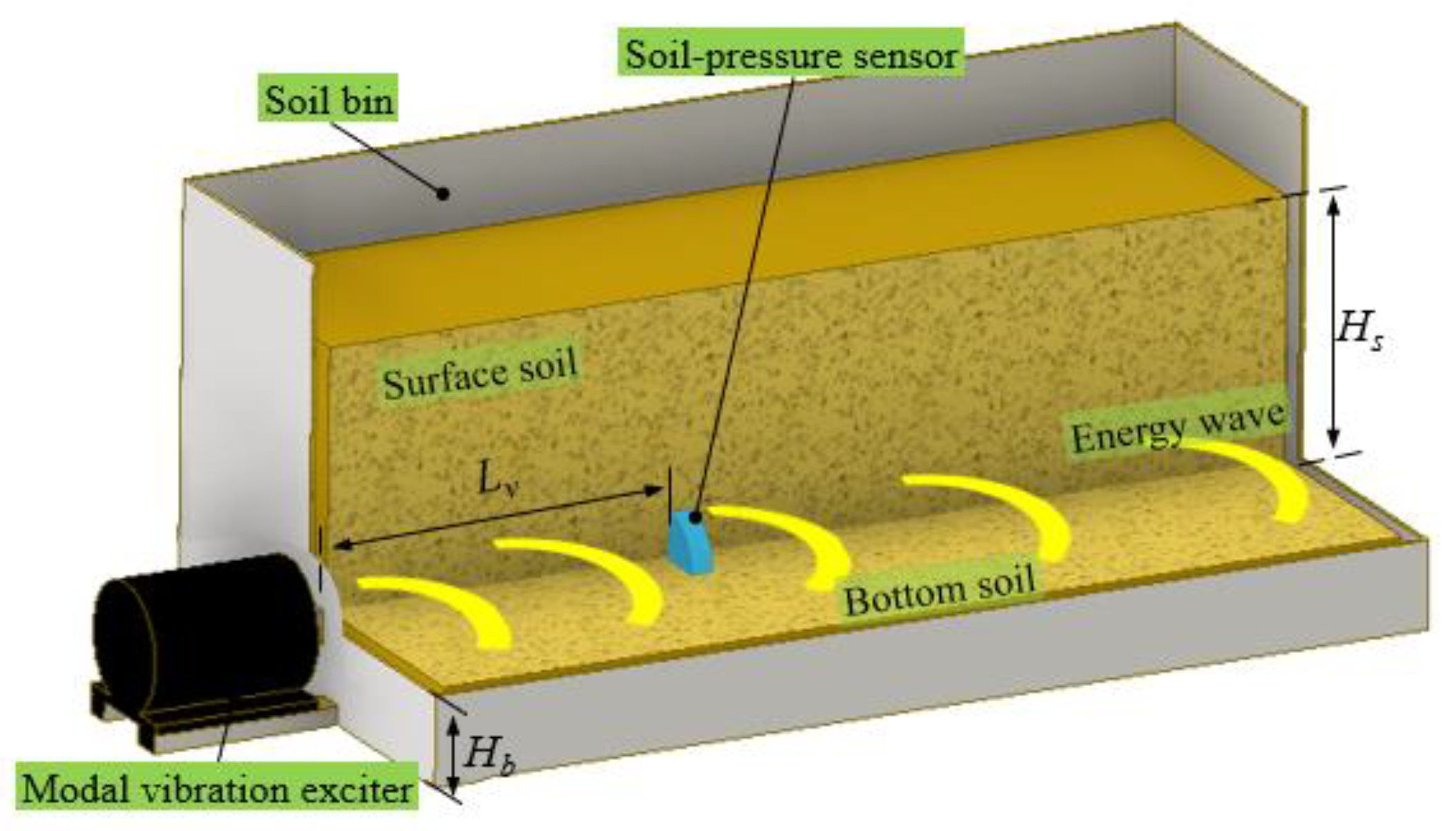
Figure 4.
The DEM model of simulation test (half sectional view of soil).
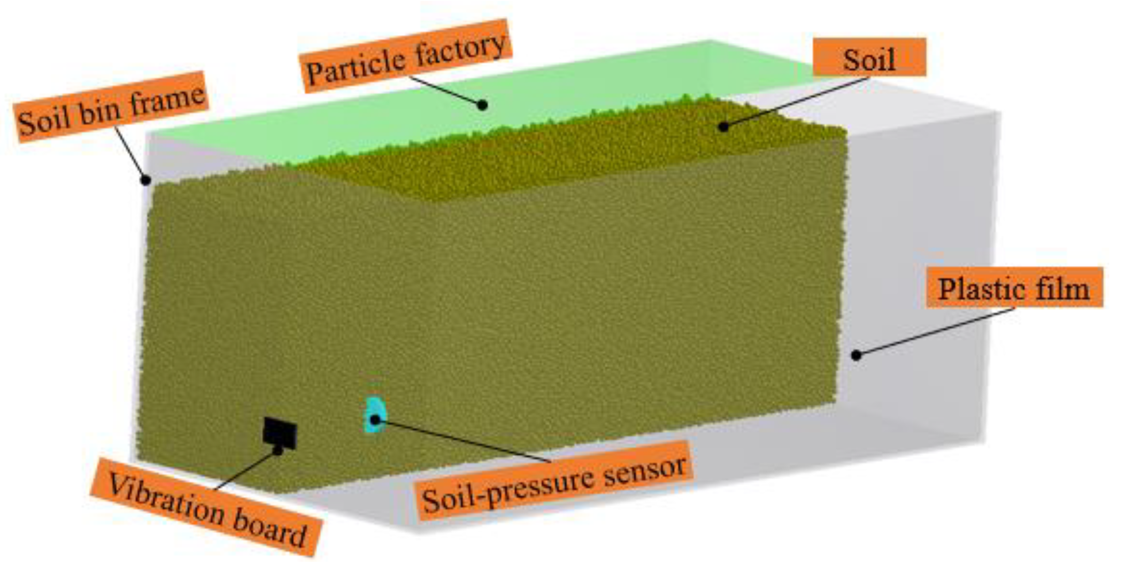
Figure 5.
Results of bench test: (a) Response curve of peak pressure and vibration frequency; (b) Response curve of pressure, vibration distance and time at 11Hz.
Figure 5.
Results of bench test: (a) Response curve of peak pressure and vibration frequency; (b) Response curve of pressure, vibration distance and time at 11Hz.
Figure 6.
Comparison of measured and simulated values at different vibration frequency: (a) 9 Hz; (b) 11 Hz; (c) 13 Hz.
Figure 6.
Comparison of measured and simulated values at different vibration frequency: (a) 9 Hz; (b) 11 Hz; (c) 13 Hz.
Figure 7.
Response curve of peak pressure and vibration distance: (a) Amplitude; (b) Vibration frequency; (c) Soil depth.
Figure 7.
Response curve of peak pressure and vibration distance: (a) Amplitude; (b) Vibration frequency; (c) Soil depth.
Figure 8.
The frequency domain response of pressure values: (a) Amplitude; (b) Vibration frequency; (c) Soil depth.
Figure 8.
The frequency domain response of pressure values: (a) Amplitude; (b) Vibration frequency; (c) Soil depth.
Figure 9.
Diagram of the cut-off pressure selection: (a) shows the pressure value versus vibration frequency response curve for each condition, and (b) shows an enlarged view of the key area.
Figure 9.
Diagram of the cut-off pressure selection: (a) shows the pressure value versus vibration frequency response curve for each condition, and (b) shows an enlarged view of the key area.
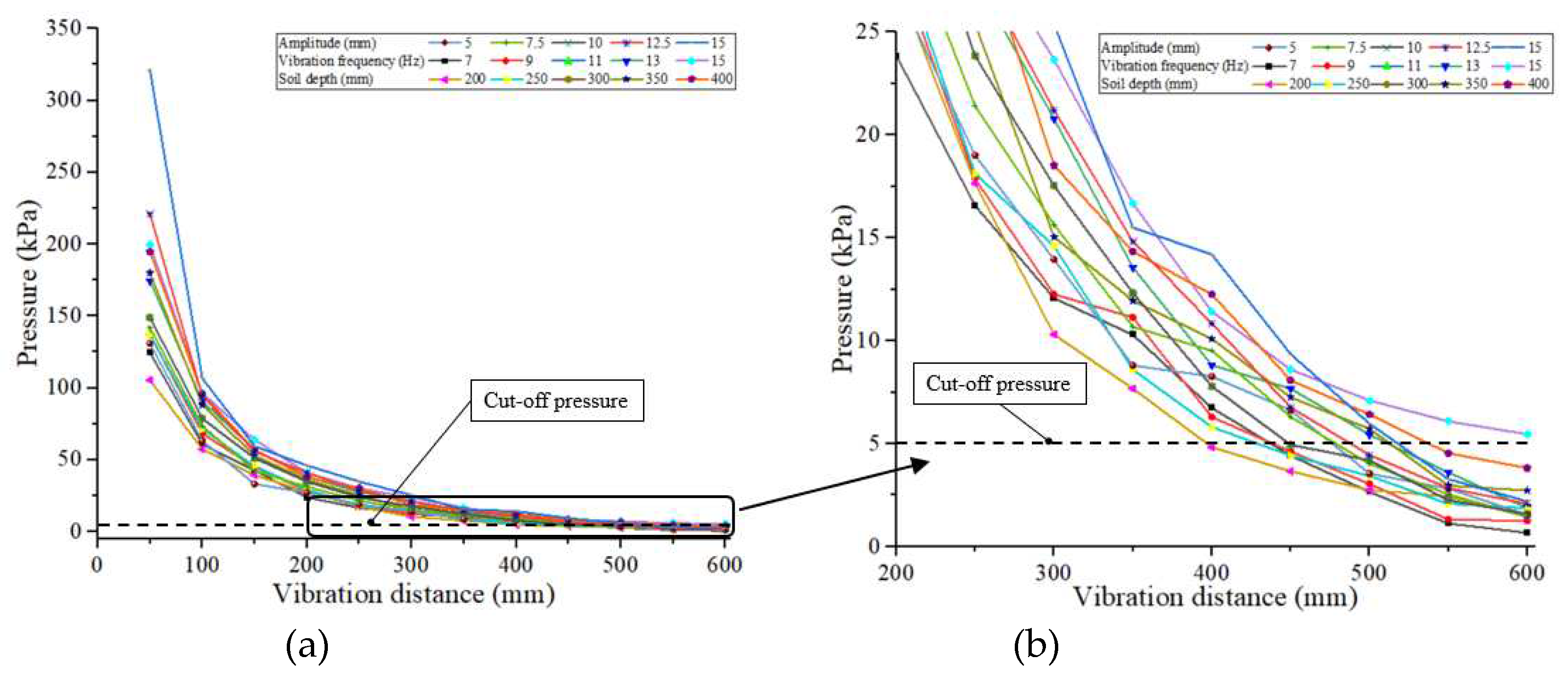
Figure 10.
Multinomial exponential function fitting curve for vibration distance and pressure: group (a) is for amplitude, group (b) is for vibration frequency and the group (c) is for soil depth.
Figure 10.
Multinomial exponential function fitting curve for vibration distance and pressure: group (a) is for amplitude, group (b) is for vibration frequency and the group (c) is for soil depth.
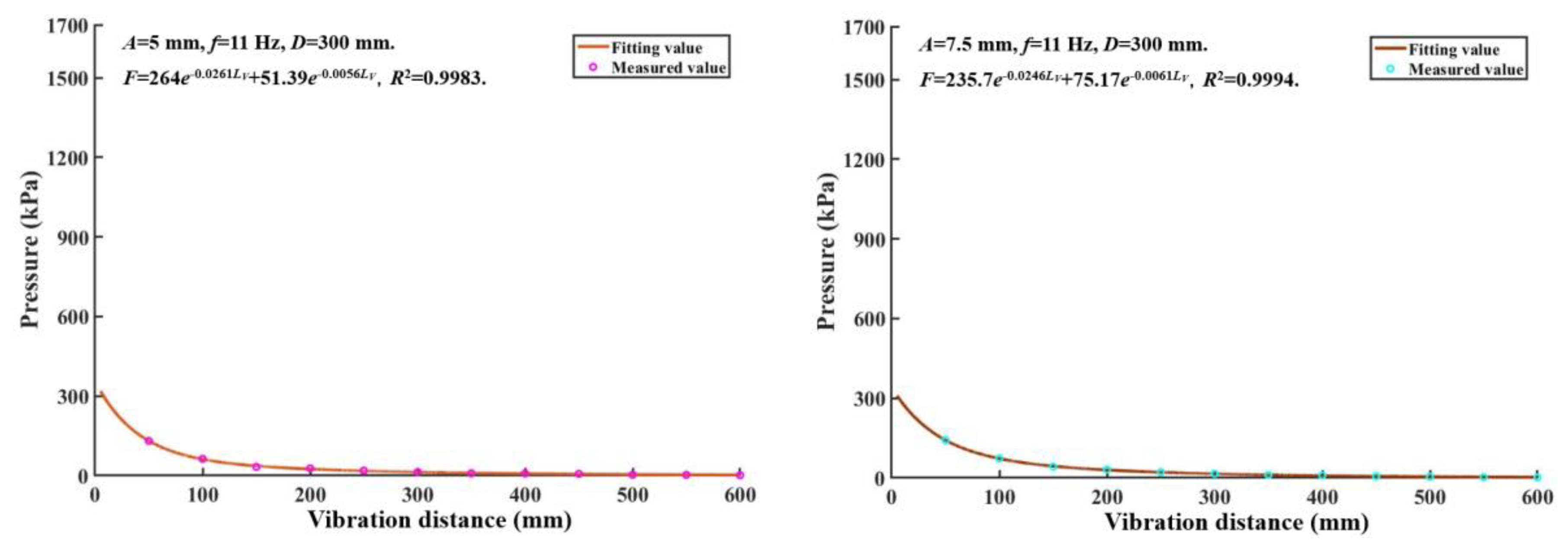
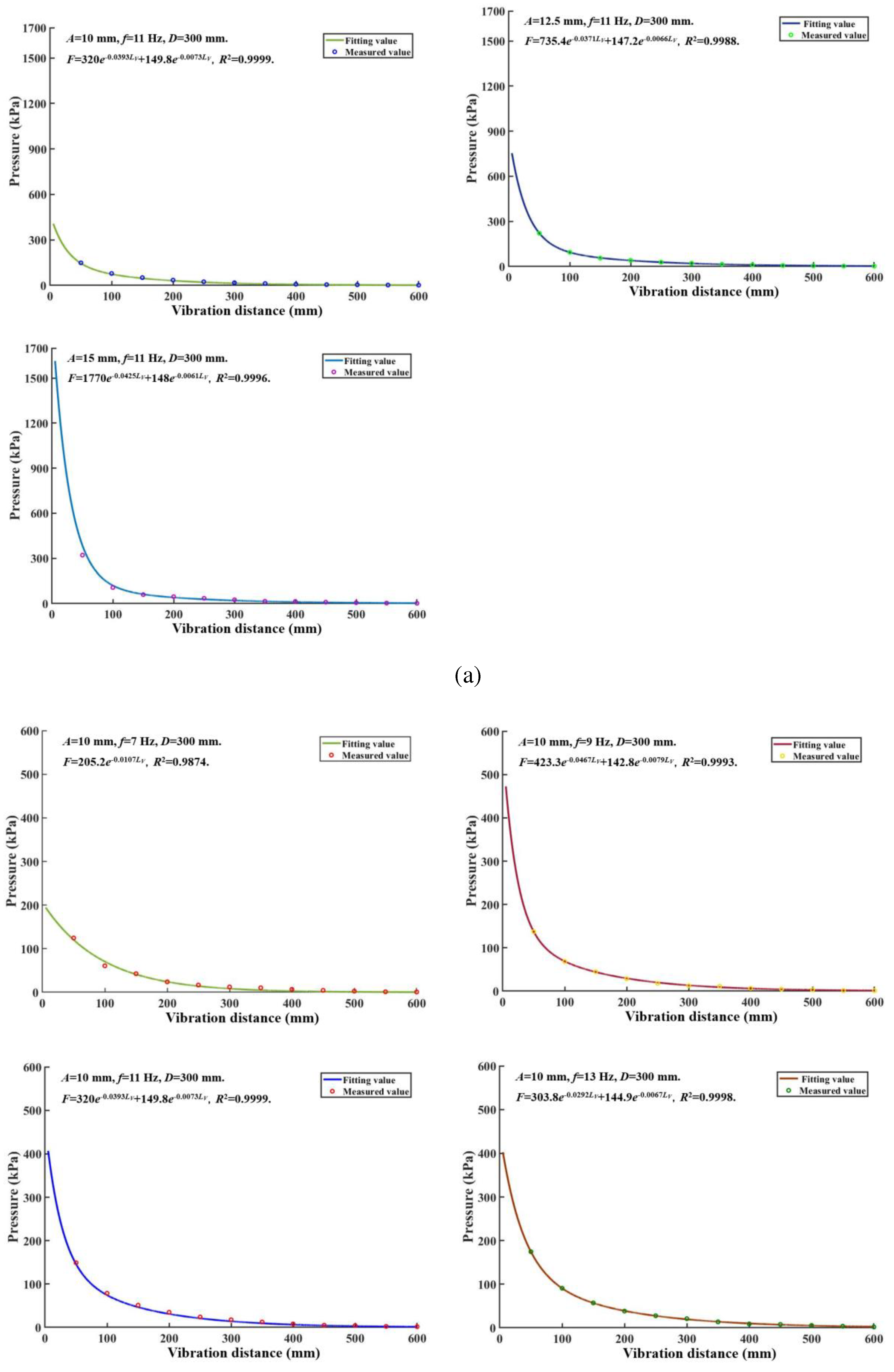
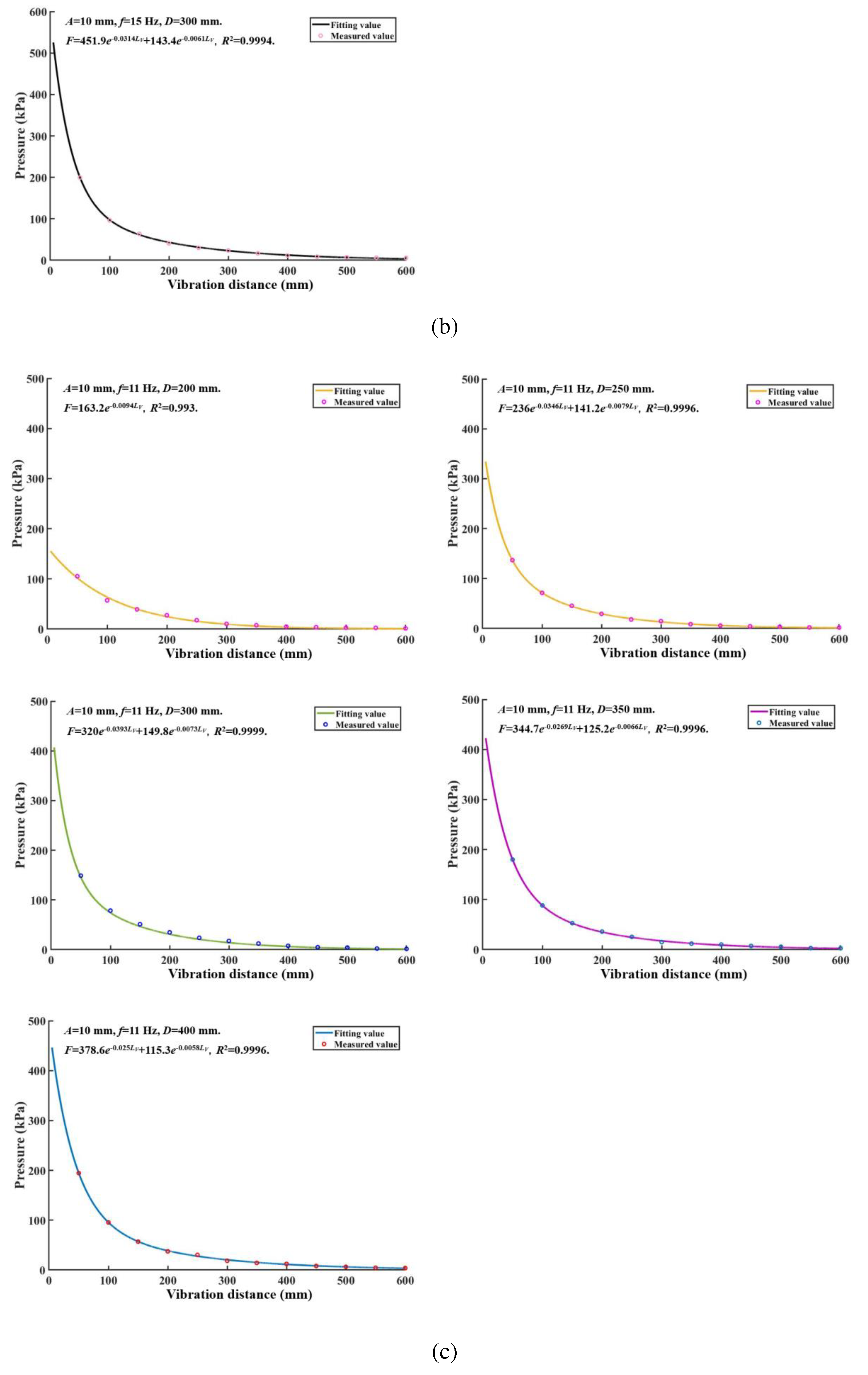
Figure 11.
Vector model of soil particles. In the front view, points a to b are the pre-loading stage, points b to point c are the loading stage, and points c to d are the pre-unloading stage. In the vertical view, points a' to b' are the pre-loading stage, points b' to c' are the loading stage, and points c' to d' are the pre-unloading stage. The black rectangular wire frame is the contact area. The black dashed line is the dividing line between the strong and weak pressure on the soil particles.
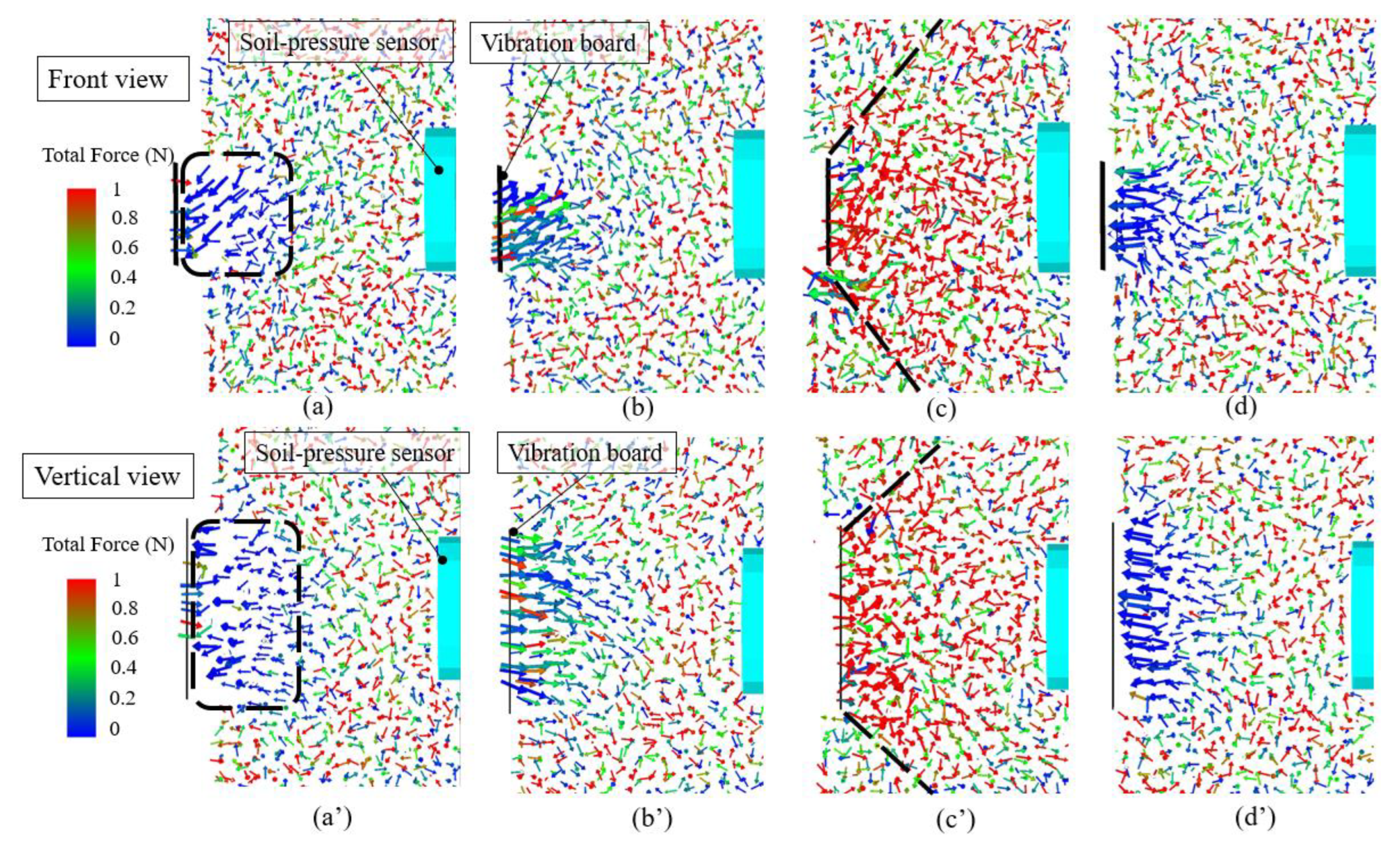

Table 1.
Contact parameters of simulation model.
| Parameters | Value | Parameters | Value |
|---|---|---|---|
| The collision recovery coefficient between soil particles | 0.25 | The bond disk radius between soil particles (mm) | 4.8 |
| The static friction coefficient between soil particles | 0.42 | The collision recovery coefficient between soil and plastic | 0.34 |
| The rolling friction coefficient between soil particles | 0.14 | The static friction coefficient between soil and plastic | 0.23 |
| The normal stiffness per unit area between soil particles (Pa) | 7.85×10⁸ | The rolling friction coefficient between soil and plastic | 0.07 |
| The tangential stiffness per unit area between soil particles (Pa) | 7.42×10⁸ | The collision recovery coefficient between soil and steel | 0.51 |
| The critical normal stress between soil particles (N) | 5.65×10⁷ | The static friction coefficient between soil and steel | 0.32 |
| The critical tangential stress between soil particles (N) | 5.39×10⁷ | The rolling friction coefficient between soil and steel | 0.09 |
Table 2.
Test factors and levels.
| Level | -2 | -1 | 0 | +1 | +2 |
|---|---|---|---|---|---|
| Amplitude (mm) | 5 | 7.5 | 10 | 12.5 | 15 |
| Vibration frequency (Hz) | 7 | 9 | 11 | 13 | 15 |
| Soil depth (mm) | 200 | 250 | 300 | 350 | 400 |
Table 3.
Dominant frequency and frequency amplitude at different amplitudes.
| Amplitude /mm | 5 | 7.5 | 10 | 12.5 | 15 |
|---|---|---|---|---|---|
| Dominant frequency /Hz | 22.17 | 22.17 | 22.17 | 22.17 | 22.17 |
| Dominant frequency amplitude /kPa | 6.73 | 7.51 | 7.91 | 10.75 | 11.99 |
Table 4.
Dominant frequency and frequency amplitude at different vibration frequencies.
| Vibration frequency /Hz | 7 | 9 | 11 | 13 | 15 |
|---|---|---|---|---|---|
| Dominant frequency /Hz | 14.78 | 17.24 | 22.17 | 12.31 | 14.78 |
| Dominant frequency amplitude /kPa | 6.52 | 7.37 | 7.91 | 11.45 | 12.03 |
Table 5.
Dominant frequency and frequency amplitude at different soil depths.
| Soil depth /mm | 200 | 250 | 300 | 350 | 400 |
|---|---|---|---|---|---|
| Dominant frequency /Hz | 22.17 | 22.17 | 22.17 | 22.17 | 22.17 |
| Dominant frequency amplitude /kPa | 6.17 | 6.72 | 7.91 | 9.48 | 10.41 |
Disclaimer/Publisher’s Note: The statements, opinions and data contained in all publications are solely those of the individual author(s) and contributor(s) and not of MDPI and/or the editor(s). MDPI and/or the editor(s) disclaim responsibility for any injury to people or property resulting from any ideas, methods, instructions or products referred to in the content. |
© 2023 by the authors. Licensee MDPI, Basel, Switzerland. This article is an open access article distributed under the terms and conditions of the Creative Commons Attribution (CC BY) license (http://creativecommons.org/licenses/by/4.0/).
Copyright: This open access article is published under a Creative Commons CC BY 4.0 license, which permit the free download, distribution, and reuse, provided that the author and preprint are cited in any reuse.


