
Submitted:
04 September 2023
Posted:
06 September 2023
You are already at the latest version
Abstract
This study addresses the challenge of objectively quantifying the value of specific views, known to provide psychological and physical benefits, from city center apartments. Unlike subjective evaluations, objective measurement is hindered by limited research and methodology. The research focuses on quantifying visibility by projecting rays from measurement points and determining whether they intersect with unobstructed views, such as the sky and natural elements. Two metrics are proposed to evaluate visibility: the number of view rays and the ratio of view rays to windows. The study analyzed 17 types of residential units in 12 complexes in northern Seoul, South Korea, with the aim of isolating the effect of views on housing prices from other factors. Correlation coefficients were used to assess the relationship between view and housing prices. The results indicated that valuations based on average visibility are more favorable than those based on maximum visibility. The amount of visibility showed a stronger correlation with apartment prices than the number of floors, suggesting the need to measure views across the entire space. The study's methodology can be applied to analyze views in different buildings and urban areas.
Keywords:
view quantification
; visibility
; ray tracing
; apartment
; apartment price
; view value
1. Introduction
A window’s view connects interior spaces to the outside surroundings, is often attractive, and can provide people with a sense of satisfaction. An appealing view not only provides aesthetic pleasure but also offers psychological comfort and physical benefits, such as aiding patient recovery, reducing stress, and increasing efficiency among office workers [1,2,3,4]. The importance of views has led to changes in standards for comfortable indoor environments that now require accessibility to views [5,6]. The real estate industry has been considering views as a premium factor for years, and the impact of views from rooms is expected to continue to grow [7,8,9].
While numerous studies have utilized interviews and questionnaires predicated on images and personal experiences to exhibit subjective evaluations of the view and its appearance through a window, there is a shortage of standardized procedures for quantitative assessments and inadequate research conducted. [2,8,10,11,12,13,14,15]. Visibility of a view is not an absolute measure of aesthetic judgment. However, the assessment of the view from a room can differ significantly depending on the extent to which an attractive view object is visible. Objective calculation and presentation of views from a space can be leveraged not just to appraise existing interior spaces but also to guide future architectural and design plans for creating superior spaces for many occupants. Moreover, an objective assessment of space based on concrete numbers will facilitate informed decisions from the perspective of occupants or buyers.
Many studies have been conducted on the real estate industry’s view premium, but most of them measure views using a dummy variable based on interviews with real estate agents or by distance to the view object [7,8,10,16,17,18,19]. However, personal judgment can lead to different valuations, and just because a house has a view doesn’t necessarily mean it has a meaningful view. Moreover, accessibility, which is determined by the distance from the viewing object, does not reflect how the object appears from inside the building. The degree of visibility varies depending on the observation location, even within the same building. Therefore, simple criteria are not enough to evaluate the view objectively. A quantitative evaluation that can indicate the actual amount of visibility will provide objective criteria, clarify the differences between each property, and allow for meaningful analysis.
The number of studies that use computers to quantify the view has increased in recent years. Kfir and colleagues [20] analyzed the view elements in the scanned photographs and calculated their area in the near, mid, and far views to evaluate the view from the unit dwelling. Numata and Obase[21] used Google Maps figures to determine the visibility of physical and view elements in a study on the effect of view on adjacent high-rise apartment prices in a redevelopment area in Japan. An alternative approach involves calculating the pixel count of a specific color in a view image and representing it as a ratio [22,23]. Nevertheless, such calculations may not account for the object’s dimensionality, since it is treated as a planar surface. Moreover, it is worth noting that getting the required images from each spot manually is necessary when measuring the viewpoint of an actual building.
On the other hand, some studies provide quantitative analyses of perspectives through geometric analysis. Since Tandy proposed isovist in 1967 [24], which quantifies and maps the amount of visibility from a particular location, there have been increasing efforts to assess the visibility of urban and architectural building spaces using geometric calculations. Benedikt utilized the isovist method by proposing numeric measures such as area–perimeter, occlusivity, variance, skewness, and circularity to quantify size and shape [25]. This method has been developed for the analysis of urban space considering not only a specific location but also movement [26]. Recently, it has become achievable to analyze the field of view in all directions and elevation angles in a GIS-based three-dimensional model that can consider topography [27,28]. However, it should be noted that in order to accurately reflect the volume of an object, the view evaluation must be based entirely on the observer’s perspective.
Visibility analysis utilizing solid angle and ray tracing is a simulation technique that involves a 3D model for precise computation and scrutiny of object geometry. It finds application in architectural, urban, and rural contexts [29,30,31,32,33,34,35,36]. In studies of apartment spaces, ray tracing is employed to analyze the viewpoint surface and assess the view by detecting object points from the viewpoint. However, this method requires effort to place the points on the surface, limiting its effectiveness [33,34]. Given that the user is not stationary and can move throughout the space, it is crucial to appraise the view from any location in the entire space rather than restricting it to a particular observation point. Especially as the distance from the window in the room increases, the proportion of the outside view it occupies decreases, and the visibility of the viewed object outside the window changes accordingly. However, a simple measure of view visibility cannot take into account this relationship. Therefore, this study proposes a window-to-view ratio that considers the visible connection between the window and the object being viewed.
In Turan and her colleges’ study [37], multiple regularly spaced measurement points are used to measure and assess the area and quantity of available views from an interior space, which are relatively large, open-plan commercial office spaces. However, to our knowledge, there are no studies that empirically assess views in residential spaces using multiple measurement points. Residential spaces are usually separated by walls rather than open-plan areas and have lower ceiling heights than commercial spaces, resulting in differences that allow for an impartial evaluation of residential environments, not only for proposed developments but also for existing buildings.
This study aims to quantitatively measure the visibility of views from residential space, particularly apartments to determine their economic value in relation to real estate prices. Applying ray tracing as in previous studies, our proposed method can measure views without placing points on the view objects detected from a viewpoint. Moreover, in terms of the view from a space rather than from a single viewpoint, this study is distinctive in that it establishes an evaluation value in terms of both the amount of view and the ratio of view to window that compiles the measurements obtained from multiple measurement points placed at regular intervals. Furthermore, we conducted an empirical evaluation of the varying relative value of views from different environments, such as mountains, parks, rivers, and building clusters, by measuring them in apartments located in urban areas.
2. Materials and Methods
2.1. Measurement of visibility
2.1.1. Concept of visibility
In this study, the state of visibility is defined as a situation in which the view object can be seen without being blocked by obstacles. The visible quantity is calculated by irradiating half-straight rays at regular intervals from the measurement point that is the viewing location and determining whether the rays intersect on the view object without being blocked by the topography, surrounding buildings, slabs, and walls of the building to be evaluated (Figure 1). The number of rays adjudicated is the visible quantity of the view object at the measurement point, and visibility is defined based on this.
2.1.2. Measurement Process
Figure 2 shows the progress of the general process of the measurement of visibility. Rhinoceros 6.0, Grasshopper for Rhino 6.0, and QGIS Desktop 2.18.20 are used as construction tools, and digital topographic maps and GIS building data are used as materials for spatial reproduction.
First, a 3D model of the building and its surroundings is developed. The terrain of the area is created based on the elevation point or contour data from a digital topographic map. Thereafter, building volumes are added to the created 3D terrain using building outlines and floor information obtained from the GIS building data. Additionally, the outer and inner walls of each room in the building are created by referring to the floor plan.
As the next step, to evaluate the view over the entire room, measurement points are placed throughout the room in this research. At this time, measurement points are arranged at certain distanced intervals considering the time required for measurement. The location of the height of the measurement points can be assumed to be the state of the standing or sitting. In this study, the interval between the measurement points is set at 1 m, and the height of the measurement points is set at 1.5 m, the standing height.
Finally, the view object and obstacles are set. In this study, the sky and natural objects (park, mountain, and river) with relatively large areas in the object area are chosen as view objects, and the topography, surrounding buildings, walls, and slabs of the subject are set as obstacles.
The view is evaluated by the extent to which the view object can be seen quantitatively. A half line radiates from the measurement point, setting the azimuth angle of the ray as θh and the elevation angle each as θv. To save calculation time, the range of radiation is set to 0 ≤ θh ≤ 360, -60 ≤ θv < 50, and the angle interval is 2° based on latitude. To ensure equal density of rays per unit solid angle, the angle of the horizontal increment Δθh is set, such that Δθh = 2/cosθv (Figure 3). Therefore, a total of 8429 rays is irradiated at each measurement point, and whether the rays intersect on the view object is investigated. The measurement model is created using GHpython, a visual programming language for Rhinoceros
2.1.3. Evaluation value of visibility
Among the studies that used the ray tracing method, those that used the method of recognizing points placed on the surface of the view object from the point of measurement evaluated the amount of view based on the number of points recognized from that point of measurement [33](Choi et al., 2014). Turan et al. expressed the percentage of total rays projected from one origin point that intersects selected outdoor landscape elements and the percentage of the analyzed area with its minimum visibility as a matrix to evaluate the entire floor [37].
In this paper, we propose two indicators for evaluating the visibility from the window: the number of viewing rays (nV) and the ratio of viewing rays to the window (RVW).
- Number of viewing rays (nV): Total number of rays that intersect the view object without being blocked by any obstacle at a measurement point. This indicates the approximate visibility of view objects at a viewpoint.
- Ratio of viewing rays to the window (RVW): Ratio of the number of rays intersecting the view object to the number of rays intersecting the window object that is considered the window area. This indicates the extent to which the view object is occupied in the external view through the window.
Viewing is achieved through the window as a medium. However, the same number of viewing rays can be seen differently in each window (Figure 4). Therefore, we propose not only the geometric visible quantity (nV) of the view object but also the ratio of the view object to the window (RVW) as an indicator for evaluation. The view may also differ depending on the shape of the window, even for the same view position. However, in this study, the height of the target room is unified, and the area of the window is considered to be the entire wall where the window is located on the floor plan; thus, the shape and height of the window are not considered.
Furthermore, viewing occurs either consciously or unconsciously in everyday life. Therefore, we do not limit the measurement points to one, but place them at regular intervals throughout the room to measure the view from the entire room. When evaluating the view of a room, the maximum (nVmax), average (nVavg), and minimum (nVmin) values of nV measured from all measurement points are representative of the room (Figure 5). Furthermore, considering the visible quantity for each depth of the room, we examine the average of nV as nVd and RVW as RVWd for each d meter of distance from the window. The standard deviation of RVW is used to examine the variation of the visible quantity throughout the room.
2.2. Case study of analysis of apartments in Seoul, Korea
2.2.1. Apartment in Korea
In Korea, apartments are a common type of residence, accounting for up to 60% of all households [38], defined as a building with five or more floors with residential functions. They have become increasingly high-rise over time, with 60% of apartments in 2017 having 15 or more floors. The development of large apartment complexes, often with thousands of units, is another feature, and each complex has its own living and commercial area.
Since Korea has many mountainous areas, even an apartment in the city center is likely to have a view of a natural object. In urban areas, properties that offer both convenience and comfort generally have a higher value than other properties. It is important to ensure convenience and comfort in the planning stage, and properties with an appropriate view are more valuable than others. In the Korean real estate industry, properties with excellent views are more expensive because of the rarity of their location. In fact, the Ministry of Land, Infrastructure, Transport, and Tourism of Korea has recognized the real estate value of the view by referring to the influence of the view as a factor in price formation [39]. Under these circumstances, the apartment transaction data are available to the public in Korea, rendering it an appropriate subject for study for examining the economic value of the view. Therefore, this study determines the amount of view available in a Korean apartment building and assesses the economic value of the view. We quantify the economic value of the view of an apartment in South Korea, especially in the northern area of Seoul.
2.2.2. View object and placement of measurement point
In this study, the visibility of two main elements is investigated. One is openness that represents the visibility of the sky, and the other is the natural landscape. The sky provides the observer with information about the passage of time, seasonal changes, and weather conditions that is also a major reason for the preference for windows [40]. This is in line with a view of openness: a wide field of view on a higher floor is preferred over a view closer to the building on a lower floor [41]. In terms of the natural landscape, a water feature is also one of the preferred landscapes; in Vecchiato’s study [42], bodies of water were chosen as the most important element to increase the visual quality of the landscape. Furthermore, a study by Zhao et al. [43] found that landscapes with approximately 45% water covered were preferred. The study of green landscapes is dealt with by various researchers, but they appeared to be less favored than water features [44]. In addition, Mirza found that the positive effect of greenery is more valuable in a view where it is obstructed than in an open view [45].
Geographically, Korea is surrounded by sea on three sides, and more than 60% of the land area is forest; thus, mountains, rivers, and the sea are the main view objects. The city of Seoul is inland; therefore, it does not have a view of the ocean, but it does have a view of mountains and rivers. The northeastern area of Seoul was chosen for this study as the area with the highest distribution of national parks and residential areas in the city. The area around the North Seoul Dream Forest Park, where the four districts included in the zone fit together, was selected. The North Seoul Dream Forest is one of Seoul’s representative parks and is surrounded by natural scenery including parks, mountains, and rivers. Six mountains and parks in northeastern Seoul were selected as view objects: Mt. Choan, Mt. Ope, Wolgye Park, Odong Park, Mt. Cheonjang, Uicheon River, and Jungnangcheon River, and North Seoul Dream Forest Park (Figure 6). In each case the sky was considered as a hemisphere, and its visibility from the measurement point was measured.
2.2.3. Case study object
Among the apartments located in this area, 17 apartment unit types in 12 apartment complexes shown in Table 1 were analyzed in this study. The objects were obtained by selecting apartments where floor plans and numerical data could be collected from the Naver Real Estate, specifically for the reasons discussed in 2.3.1 [46]. The surfaces of geography and buildings were created based on the digital topographic map and GIS building information provided by the National Geographic Information Institute in Korea as of 2019 [47]. To shorten the calculation time, the 3D models including the surrounding environment with a radius of 1 km around each object apartments were created to investigate the visibility of the view. The building dimensions have been extracted from the GIS building information conveying only the footprint and height of the building. For simplification purposes, all object apartments are set to 0.2 m width for the exterior walls and 0.15 cm width for the interior walls, with a floor height of 3 m and a ceiling height of 2.5 m. The measurement points are set to the living room of each apartment unit since it has the largest opening and is the main living place of the family members. The height of points is set at 1.5 m, considering eye height standing with 1 m intervals. In most Korean apartments, an enclosed balcony (veranda) is usually placed between the living room and the outside. It is often used to expand the living room by eliminating the wall between; therefore, the measurement points are also placed on the enclosed balcony in this measurement. The view measurement results for the object apartments are shown in 3.1.
2.3. Comparison with actual transaction price
In this study, the economic values of visibility of view for each apartment unit are analyzed by comparing them with the actual transaction price. The hedonic pricing model is applied for the analysis. The transactions are from 2006 to 2019 and collected for the relevant properties from the actual transaction price disclosure system [48] published by the Ministry of Land, Infrastructure, and Transport in Korea (MOLIT).
2.3.1. Outline of the actual transaction price data
The actual transaction price data from MOLIT includes information of address and name of an apartment complex, net floor area, date, price, and number of floor level of transactions. However, since building number and room number are not included in the data, it is not available for identification of the location if the same apartment type with the same net floor area exists in different buildings in the complex or on the same building plane. In this study, only the apartments in the apartment complex, i.e., the apartment types that exist only in the complex and on each building plane, are targeted. Total 17 cases of apartment types where the natural view object exists within a radius of 1 km in the target area and its location can be identified in the apartment complex are selected, and total 235 transaction data are collected. The selection of apartment units is conducted using the information on real estate complexes provided by NAVER, a website in South Korea[46].
2.3.2. Estimation of view value in apartment price
This section explains the equation for examining the economic value of view using the measured visibility of view and actual transaction price data. Hedonic price models are commonly used to estimate certain values included in the price of a house [49](Rosen, 1974). Hedonic models exist in various forms, with linear and semi-log models being commonly used. The semi-log function allows for variation in the value of certain characteristics, such that the price of one component is partially dependent on the other characteristics of the dwelling [50]. In this study, the semi-log that incorporates natural logarithm prices and linear independent variables has been adopted to account for the possibility that view prices are affected by other characteristics.
The price of an apartment unit i ( = 1, 2, …), Pi is determined by various factors Xij (j = 1, 2, …), such as structural, locational, neighborhood, and environmental characteristics [51,52,53]. A view comprises a combination of various elements, including the sky, natural objects such as mountains, oceans, rivers, and parks, and man-made buildings that can be considered obstructions. Considering the influence of visibility of view Vi, that is, the impact of the extent of sky or natural object visible from the room on the apartment price, the price of an apartment can be estimated as follows: (1) α and β are the coefficients of each variable, and ϵ is the error term.
High-rise apartments often have the same floor plan vertically. Thus, they share the same floor plan on the vertical side within a single building and are the subject of this study. Given a transaction for apartment unit a and apartment unit b in the same unit type, subtract both sides of Equation (1) for each transaction price Pa and Pb. They have the same structure, location, neighborhood, and environmental characteristics, implying Xaj = Xbj for all j. Therefore, we can eliminate the influence of multiple factors and obtain an equation in which only the view affects the price (2). The difference between the price of the apartment and the amount of visibility remains at both ends, and the effect of the amount of visibility on the apartment price is analyzed by examining the correlation coefficient (R) between the two values. For those visibility quantities that are each zero, the difference between the two views is unknown; thus, it is excluded when calculating the correlation coefficient.
However, prices are generally influenced significantly by economic conditions at time t. When P’it is the actual transaction price of apartment unit i at a certain time t, the transaction price Pit used in this study is the actual transaction price divided by the Apartment Housing Index AHIt per square meter based on exclusive private area (EPA) (3). AHI is a monthly index of actual apartment transaction prices provided by the Korean Statistical Information Service (KOSIS)[54], particularly for the northeast region of Seoul.
In addition, considering the possibility that the influence of the rapid fluctuation of apartment prices in Korea has not been fully eliminated, the transaction time ti for property i and apartment unit a and b to be subtracted, the transaction time difference |ta-tb| is set to a maximum of 6 months.
The number of transactions and the number of possible calculations made in one apartment unit type are presented in Table 2. To obtain significant correlation coefficients from them, the apartment unit types were selected, such that the number of possible calculations is at least 10. The results of the correlation coefficient between the actual transaction price and the above view are shown in 3.2.
3. Results
3.1. View evaluation results
This section summarizes the results of 17 research subjects that measured the visible amount of view objects. We present an example of the measurement results for G2, a typical Korean family-type 3-bedroom unit that is close to the average residential apartment gross floor area (74.6 m2), from the 2017 Korean Population Housing Survey.
3.1.1. Evaluation of case G2
Apartment unit G2 has 15 floors, with the living room facing northern east. Choan Mountain, Yeongchuk Mountain, and Uicheon River were set as the natural view object; among them Choan Mountain is located relatively close to the measurement point relative to other view objects (Figure 7). For measuring visibility, total 15 measurement points were placed in the living room on each floor (Figure 8).
Figure 9 shows the boxplot of the visibility of sky on each floor. Maximum (nVmax), minimum (nVmin), and average (nVavg) of nV are gradually increased with the increase in floor level. It was confirmed that the higher the floor, the better the view of the sky. Throughout all floors, more than 75% of the measurement points showed less than half that amount visible compared with the maximum. This indicates that the sky is unevenly visible at this property.
Figure 10 shows the nVd of each floor. The visible quantity decreased with increasing distance from the window. However, the decrease was more severe in front of the window than at the back of the room. For example, on the 15th floor, nV decreases by approximately 500 when the distance from the window increases from 1 m to 2 m, whereas nV decreases by approximately 50 when the distance from the window increases from 4 m to 5 m. It can be said that the visible quantity of sky in the room is considerably better in the window side than at other locations.
RVWd of sky is shown in Figure 11 for each floor. RVWd decreases with increasing distance from the window, but the degree of decrease is moderate compared with nVd. A difference in the ratio of decrease with distance from the window between the upper and lower floors is also observed. The top floor (15F) showed a decrease of approximately 10%, while the bottom floor (1F) showed a decrease of approximately 28% when the distance increased from 1 m to 5 m. Compared with the lower floors, the upper floors can be said to have a larger percentage of sky in the windows when viewed from a distance through the windows.
On the heatmap of nV and RVW at each measurement point (Figure 12), nV is concentrated on the window side throughout all floors. However, the standard deviation of RVW decreases with the upper floors, that on the first floor is 10.80, while that on the 15th floor is 4.09. The sky viewed from inside the room varies according to its viewing position, but the higher the floor, the smaller the variation in the percentage of sky in the window within the living room.
Figure 12.
Heatmap of nV and RVW of sky on each measurement point of G2.

The most detected view object in this apartment unit is Choan Mountain, while Ui River is not detected at all (Figure 13). Only Choan Mountain and Yeongchuk Mountain were considered as the natural view object.
Maximum (nVmax), minimum (nVmin), and average (nVavg) of nV gradually increase as the floor level increases, and their values decrease after the maximum value is reached at a certain floor. The floors where nVmax, nVmin, and nVavg reach their respective maximum values are different, with nVmax being 1353 on the 13th floor, nVavg being 586 on the 10th floor, and nVmin being 241 on the 5th floor (Figure 14). Comparing by floor, the maximum and minimum ranges are wider on the upper floor than on the lower floor. This indicates that on the upper floors, certain areas have the greatest view of the view object compared with the other floors, while other areas do not afford such a view for natural objects.
The average of natural object (nVd) visibility according to the distance from window of each floor is shown in Figure 15. The nVd of natural view object decreases as the distance from the window increases. However, the decrease was more severe with the increase in the number of floors. This indicates that in the upper floors, the view object is less visible on the far side than on the window side, and even less in the lower floors. Compared with the sky in Figure 10 that exhibits extremely high nV near the windows for all floors, the natural object shows less variation in the visible quantity depending on the viewer’s position on different floors.
In terms of the ratio to the window area, a higher ratio was obtained at the back of the window than at the window side. The maximum RVWd of 92.01 was obtained on the 5th floor at the measurement points 5 m away from the window, indicating that the window is almost occupied by natural objects (Figure 16). The degree to which RVWd increases as the distance away from the window increases varies from floor to floor. Compared with the sky that shows a tendency for the ratio to decrease at the far end of the room (Figure 11), the opposite is observed for the natural object.
The variation was greatest on the fifth floor with respect to the occupancy of view seen through the window area (standard deviation = 23.54) (Figure 17). It is more likely than on other floors that the appearance of the view object varies depending on the position from which the viewer looks outside. Compared with the sky that shows higher variability on the lower floors and lower variability on each upper floor (Figure 12), the natural object shows lower variability even on the lower floors.
3.1.2. Summary of 17 apartment units
3.1. Economic value of view visibility
The correlation coefficient (R) between the difference in transaction price and the amount of view from the property in question is used to determine the extent of impact of the view on the price of the apartment. Table 5 summarizes the correlation coefficients for eight apartment unit types. The correlation coefficients (Rmax, Ravg) were calculated based on the maximum and average of the sky and natural objects as the viewable objects. To clarify the effect of the view on the price, correlation coefficients (Rfl) with the difference in the number of floors were also obtained, excluding the effect.
The results obtained showed that C, E1, E2, and N1 did not yield valid correlation coefficients from both sky and natural objects. Only A and O1 showed valid correlation coefficients for both sky and natural objects. G2 showed a valid correlation coefficient for natural objects only, and M showed no correlation coefficient because no natural objects were visible, but a valid correlation coefficient for sky was obtained.
4. Discussion
4.1. View evaluations on each apartment unit
There were three cases where both the sky and the natural object were visible for all measurement points arranged: E1, E2, and O1. Five of the cases included measurement points where only the sky was visible for all measurement points: A, C, D, K2, and V3. Conversely, there were four cases where only the natural object was visible for all measurement points: G1, G2, G3, and J2. Five cases exhibited nV less than 15 for all measurement points, where the natural object was almost invisible: K1, M, N1, T2, and V3. Among them, M and T2 included measurement points where even the sky was not visible.
The most visible measurement point for the sky was located on the highest floor in all 17 units, while only 8 units were for natural objects. This indicates that the sky is most visible at higher locations, while the natural object is not necessarily most visible at higher locations, but rather in a specific floor. This may be related to natural objects having a fixed physical form, as opposed to the sky having an infinite form. Generally, the obstacles, that is, the buildings between the subject building and the natural object that block the view, decrease as the floor level increases. However, along with the distance and the reduction of the prospective angle to natural object from a certain floor, the area blocked by the floor structure of the room in question may exceed the visible area.
On average, for the sky, generally the top floor with the most visible viewpoint was the most visible floor of the unit. However, for natural objects, on average, the most visible floor did not coincide with the floor with the most visible viewpoint and in fact, was below it. This is related to the following case: when viewing from the back of a room, the object visible in the lower floor may be blocked by the floor structure and not be visible in the upper floor, such that the sum of visibility to the view from the entire room may be greater in the lower floor than in the upper floor.
4.2. Economic value of view visibility
Regarding the sky, there were negligible differences observed for Rmax and Ravg (Figure 18). This reveals that when assessing the economic worth of a sky view, there is minimal distinction between utilizing either the maximum or average value as the index. The correlation coefficients between the number of floors, visible quantities, and their corresponding transaction prices showed no significant difference (refer to Figure 19). One can assume that the economic value of a sky view is analogous to that of the floor number. According to Masoudinejad and Hartig’s research on the matter of price, the sky is reported as a positive attribute [55]. It is speculated that the gradual elevation in the amount of sky visible from higher floors may reflect subconscious value in people’s minds relating to the number of floors.
Figure 18.
Comparison of the maximum (a) and average (b) of the visibility of the correlation coefficient with transaction price of each apartment unit.
Figure 18.
Comparison of the maximum (a) and average (b) of the visibility of the correlation coefficient with transaction price of each apartment unit.
Figure 19.
Comparison of the maximum (a) and average (b) of the visibility and the floor number of the correlation coefficient with transaction price of each apartment unit against the sky.
Figure 19.
Comparison of the maximum (a) and average (b) of the visibility and the floor number of the correlation coefficient with transaction price of each apartment unit against the sky.
Regarding the view of natural objects, A showed a stronger correlation with the number of floors to the transaction price, while G2 and O1 showed a stronger correlation with the visible quantity to the transaction price (refer to Figure 20). This finding suggests that for A, the number of floors is more influential in determining the transaction price than the view, whereas for G2 and O1, the view plays a more critical role (refer to the above sentence). A’s location is nearer to the subway station but relatively further from the natural object, whereas G2 and O1’s location is further from the station but closer to the natural object (refer to Figure 6). Taking into account that G2 and O1 have more extensive views due to their proximity to the view object, it appears that the apartment’s actual price is more likely to mirror the view’s actual value than in A, where the view object is further away. In contrast to G2 and O1, A appears to be priced according to the number of floors based on the conventional belief that higher floors offer a better view, instead of considering the visible extent of the view. Specifically, the findings in G2, where mountains are predominantly visible, differ from Jim and Chen’s evaluation of mountains, which reveals a negative premium when utilizing hedonic analysis with view as a dummy variable [52,56,57]. Although these differences could be accounted for by varying cultural and regional outlooks on the view object, the significance of utilizing an objective measure of view quantity in valuation should also be taken into consideration.
Figure 20.
Comparison of the maximum (a) and average (b) of the visibility and the floor number of the correlation coefficient with transaction price of each apartment unit against the natural object.
Figure 20.
Comparison of the maximum (a) and average (b) of the visibility and the floor number of the correlation coefficient with transaction price of each apartment unit against the natural object.
5. Conclusions
To evaluate the economic value of view from residential apartments in the city center, we attempted to quantify it based on the view visibility. It was adapted to a total of 17 apartments in actual architectural space, and the amount of the view was measured mainly in the living room. The evaluation was performed based on the maximum, average, minimum, and evenness of the view of sky and natural objects such as mountains, parks, and rivers in each unit. We used the maximum and average values as representative values, comparing them to the actual transaction prices to determine the economic value.
When analyzing the economic value of view over the actual transaction price, we modified the equation of the hedonic model to determine the effect of the view factor alone on the price of the apartment. Two main results were obtained:
First, the economic value of the sky view from the room does not differ considerably when determining the criterion of maximum or average amount of view. However, in the case of natural objects, a more positive result may be obtained if the valuation is based on the average amount of view.
Second, the economic value of the sky view may not differ from the economic value of the number of floors. Furthermore, for natural objects, given that the visible quantity shows a higher correlation with house price than with the number of floors, it is reasonable to measure the view throughout the entire room.
Nonetheless, since this study’s scope was limited to a relatively small number of apartments and transactions, more dependable analysis based on performance of demonstration tests in different areas and apartments is warranted. Thus, since the openings in this study were set as full windows, analysis of views relative to size and shape should be conducted in future studies. In addition, although we were able to analyze the amount of visibility to the view object, we did not consider view value to distance; this will be studied in the near future.
This study objectively assessed views using geometric analysis through simulation. Although the view is limited to the sky and natural objects, it is possible to study the amount of visibility for multiple objects depending on the target setting. By calculating the ratio of the view to the window as well as the physical quantity of the view, it was possible to analyze the view from various perspectives. This approach is useful not only for houses but also for buildings with diverse purposes, as well as for urban areas. Its significance lies in its ability to study views from multiple perspectives. This study is significant as it offers criteria for achieving sustainable development in diverse urban settings, particularly those experiencing rapid growth. This ensures better indoor spaces for the people while preserving natural landscapes.
Author Contributions
Conceptualization, H.P.; methodology, H.P., T.A. and K.H.; software, H.P. and T.A.; validation, H.P., T.A.,K.H. and K.I.; formal analysis, H.P.; investigation, H.P.; resources, H.P.; data curation, H.P.; writing—original draft preparation, H.P.; writing—review and editing, H.P., T.A.,K.H. and K.I.; visualization, H.P.; supervision, K.I.; project administration, H.P.; All authors have read and agreed to the published version of the manuscript.
Funding
This research received no external funding.
Institutional Review Board Statement
Not applicable.
Informed Consent Statement
Not applicable.
Data Availability Statement
Data is contained within the article.
Conflicts of Interest
The authors declare no conflict of interest.
References
- Ulrich, R. S. Effects of gardens on health outcomes: Theory and research. In Healing gardens: Therapeutic benefits and design recommendation, Marcus, C. C., & Barnes, M., Eds.; New York: John Wiley & Sons, 1999; Volume 4, pp. 27–86).
- Shin, W. S. The Influence of Forest View through a Window on Job Satisfaction and Job Stress. Scandinavian Journal of Forest Research 2007, 22 (3), 248–253. [Google Scholar] [CrossRef]
- Abd-Alhamid, F.; Kent, M.; Calautit, J. K.; Wu, Y. Evaluating the Impact of Viewing Location on View Perception Using a Virtual Environment. Building and Environment 2020, 180, 106932. [Google Scholar] [CrossRef]
- Ko, W. H.; Schiavon, S.; Zhang, H.; Graham, L. T.; Brager, G.; Mauss, I. B.; Lin, Y. C. The Impact of a View from a Window on Thermal Comfort, Emotion, and Cognitive Performance. Building and Environment 2020, 175, 106779. [Google Scholar] [CrossRef]
- European Committee for Standardization Technical Committee CEN/TC 169. European Standard EN 17037:2018 Daylight in buildings, 2018.
- U.S. Green Building Council. LEED v4.1 Building Design and Construction; Green Building Information Gateway; Washington D.C., 2022.
- Luttik, J. The Value of Trees, Water and Open Space as Reflected by House Prices in the Netherlands. Landscape and Urban Planning 2000, 48 (3–4), 161–167. https://doi.org/10.1016/s0169-2046(00)00039-6. [CrossRef]
- Jim, C. Y.; Chen, W. Y. Value of Scenic Views: Hedonic Assessment of Private Housing in Hong Kong. Landscape and Urban Planning 2009, 91 (4), 226–234. https://doi.org/10.1016/j.landurbplan.2009.01.009. [CrossRef]
- Damigos, D.; Anyfantis, F. The Value of View through the Eyes of Real Estate Experts: A Fuzzy Delphi Approach. Landscape and Urban Planning 2011, 101 (2), 171–178. https://doi.org/10.1016/j.landurbplan.2011.02.009. [CrossRef]
- Yoshida, M.; Yokouchi, N.; Sakurai, S.; Shizuno, T. A Study on the Appraisal on Views Commanded from High-Rise Apartments. Toshi Keikaku Rombunshū 1997, 32 (0), 487–492. https://doi.org/10.11361/journalcpij.32.487. [CrossRef]
- Lee, G. T.; Lee, J. Y. 도시 이미지로서 낙동강 수변공간의 아파트 단지의 조망경관분석에 관한 연구 (A Study on Analysis of View-Character of Apartment Site near Waterfront of River Nakdong as Urban Image). 대한건축학회 논문집 - 계획계 (Journal of the Architectural Institute of Korea Planning & Design) 2001, 17 (9), 261–272.
- Demura, Y.; Kawasaki, M. 近代吉田山の丘陵地開発における景観デザインに関する研究 (The Landscape Design for Development on the Yoshidayama Hillside in Modern Era). Journal of Civil Engineering and Planning 2003, 20, 409–418. https://doi.org/10.2208/journalip.20.409. [CrossRef]
- Moon, J. W.; Ha, J. M. 조망 대상과 조망 위치에 따른 아파트 조망 경관 선호도 특성 분석 (Preference Analysis of the View from Apartment according to View Target and Viewing Location). Journal of the Architectural Institute of Korea Planning & Design 2005, 21(5), 151–158.
- Matusiak, B.; Klöckner, C. A. How We Evaluate the View out through the Window. Architectural Science Review 2015, 59 (3), 203–211. https://doi.org/10.1080/00038628.2015.1032879. [CrossRef]
- Lin, T.; Le, A.; Chan, Y. Evaluation of Window View Preference Using Quantitative and Qualitative Factors of Window View Content. Building and Environment 2022, 213, 108886. https://doi.org/10.1016/j.buildenv.2022.108886. [CrossRef]
- Benson, E. D.; Hansen, J. L.; Schwartz, A. L.; Smersh, G. T. Ricing Residential Amenities: The Value of a View. Journal of Real Estate Finance and Economics 1998, 16 (1), 55–73. https://doi.org/10.1023/a:1007785315925. [CrossRef]
- Shin, S. Y.; Kim, M. H.; Mok, J. H. 서울숲 조성이 주택가격에 미치는 영향 (The Effects of Seoul Forest Project on Neighborhood Housing Prices). Seoul Studies 2006, 7 (4), 1–1.
- Jung, T. Y.; Baek, Y.; Sohn, J.; Yoo, S. The Effect of an Urban Park View on the Price of Apartment - A Case of Songdo Central Park -. 환경영향평가 (J. Environ. Impact Assess) 2016, 25 (6), 457–465. https://doi.org/10.14249/eia.2016.25.6.457. [CrossRef]
- Bea, S. Y.; Jo, A. H.; Lee, S. Y. 한강변 입지와 단위세대의 층수가 주택가격에 미치는 영향-서울시 아파트를 중심으로– (Effect of spatial proximity to Han riverside and Floor number on Apartment Price in Seoul). Seoul Studies 2018, 19(1), 21–40. https://doi.org/10.23129/seouls.19.1.201803.21. [CrossRef]
- Kfir, I. Z.; Munemoto, J.; Sacko, O.; Kawasaki, Y. EVALUATION OF THE VIEW FROM THE DWELLING UNITS ON MAN MADE ISLANDS IN OSAKA BAY : Multiple Regression Analysis Based on Residents’ Evaluation and Image Processing of Photographs Taken from the Living Room. Journal of Architecture,Planning and Environmental Engineering 2002, 67 (554), 357–364. https://doi.org/10.3130/aija.67.357. [CrossRef]
- Numata, M.; Obase, R. 超高層マンションにおける眺望景観が開発者の価格評価に及ぼす影響(EFFECT ON A DEVELOPER’S ESTIMATING PRICE OF THE SCENIC VIEWS IN THE SUPER-HIGH-RISE RESIDENCE). Journal of Architecture,Planning and Environmental Engineering 2010, 75 (652), 1499–1506. https://doi.org/10.3130/aija.75.1499. [CrossRef]
- Moon, K. H.; Ahn, H. T.; Kim, J. T. 그래픽 프로그램을 이용한 조망권 분석기법 (Evaluation Methodology of View Right Using Graphic Programs). The Journal of The Korea Institute of Ecological Architecture and Environment 2007, 7 (2), 9–15.
- Jung, J. H.; Kim, S. Y. 공동주택 계획단계 세대별 조망분석 및 평가에 관한 연구 (A Study on the Analysis Technique and Evaluation Method of the View from Inner Side of Apartment Housing on the Planning Stage of Layout). Journal of the Architectural Institute of Korea Planning & Design 2010, 26(10), 261–270.
- Tandy, C. R. V. The isovist method of landscape survey. In Methods of Landscape Analysis, Murray, C.R., Ed.; Landscape Research Group: London, 1967; pp9–10.
- Benedikt, M. To Take Hold of Space: Isovists and Isovist Fields. Environment and Planning B: Planning and Design 1979, 6 (1), 47–65. https://doi.org/10.1068/b060047. [CrossRef]
- Batty, M. Exploring Isovist Fields: Space and Shape in Architectural and Urban Morphology. Environment and Planning B: Planning and Design 2001, 28 (1), 123–150. https://doi.org/10.1068/b2725. [CrossRef]
- Llobera, M. Extending GIS-Based Visual Analysis: The Concept of Visualscapes. International Journal of Geographical Information Science 2003, 17 (1), 25–48. https://doi.org/10.1080/713811741. [CrossRef]
- Yang, P. P.; Putra, S. Y.; Li, W. ViewSphere: A GIS-Based 3D Visibility Analysis for Urban Design Evaluation. Environment and Planning B: Planning and Design 2007, 34 (6), 971–992. https://doi.org/10.1068/b32142. [CrossRef]
- Ohno, R. 環境視の概念と環境視情報の記述法 (CONCEPT OF AMBIENT VISION AND DESCRIPTION METHOD OF AMBIENT VISUAL INFORMATION : A Study on Description Method of Ambient Visual Information and Its Application (Part 1)). Journal of Architecture, Planning and Environmental Engineering (Transactions of AIJ) 1993, 451 (0), 85–92. https://doi.org/10.3130/aijax.451.0_85. [CrossRef]
- Honma, Y.; Kurita, O.; Suzuki, A. 計算幾何学アルゴリズムに基づく立体角指標を用いた都市景観評価 (AN ANALYSIS OF URBAN LANDSCAPES WITH RESPECT TO SOLID ANGLES BASED ON COMPUTATIONAL GEOMETRY ALGORITHMS). Journal of Architecture,Planning and Environmental Engineering 2009, 74 (643), 2035–2042. https://doi.org/10.3130/aija.74.2035. [CrossRef]
- Hirasawa, Y.; Ukai, T.; Kurita, O. 歩行者の位置と視線を反映した並木の緑視率(Ratio of Visible Green Associated with Pedestrian Location and Visual Line). Journal of the City Planning Institute of Japan 2017, 52 (3), 1276–1283. https://doi.org/10.11361/journalcpij.52.1276. [CrossRef]
- Domingo-Santos, J. M.; De Villarán, R. F.; Rapp-Arrarás, Í.; De Provens, E. C. The Visual Exposure in Forest and Rural Landscapes: An Algorithm and a GIS Tool. Landscape and Urban Planning 2011, 101 (1), 52–58. https://doi.org/10.1016/j.landurbplan.2010.11.018. [CrossRef]
- Choi, Y. S.; An, K. H.; Kim, Y. S.; Lee, J. C.; Kim, I. S. BIM을 이용한 조망권 정량화에 관한 연구 (A Study on the quantification of ‘prospect right’ using B.I.M.). 2014 FALL CONGRESS KOREA PLANNING ASSOCIATION 2014, 34(2), 57–58.
- An, K.; Choi, Y. 중정형 공동주택(아파트)의 조망계획에 관한 연구(A Study on the View Plan of Courtyard Apartment). Journal of the Architectural Institute of Korea Planning & Design 2017, 33 (4), 3–10. https://doi.org/10.5659/jaik_pd.2017.33.4.3. [CrossRef]
- Sato, T.; Takatori, A.; Satoh, Y. 可視率を用いた観客席設計のための舞台への見通し評価手法に関する研究 (VISIBILITY EVALUATION METHOD FOR AUDITORIUM DESIGN USING VISIBLE AREA RATIO). Journal of Architecture,Planning and Environmental Engineering 2017, 82 (737), 1695–1702. https://doi.org/10.3130/aija.82.1695. [CrossRef]
- Honma, K.; Imai, K. 視対象のある部屋のビジビリティに基づく形状最適化(SHAPE OPTIMIZATION OF ROOMS WITH A VISUAL TARGET TO MAXIMIZE ITS VISIBILITY). Journal of Architecture,Planning and Environmental Engineering 2019, 84 (759), 1113–1122. https://doi.org/10.3130/aija.84.1113. [CrossRef]
- Turan, I.; Chegut, A.; Fink, D.; Reinhart, C. Development of View Potential Metrics and the Financial Impact of Views on Office Rents. Landscape and Urban Planning 2021, 215, 104193. https://doi.org/10.1016/j.landurbplan.2021.104193. [CrossRef]
- Population and Housing Census, 2017. Statistics Korea. https://kostat.go.kr/anse/.
- Criteria for Investigation and Calculation of Apartment Price, 2016. Ministry of Land, Infrastructure, and Transport, Korea (MOLIT). https://www.law.go.kr/LSW/admRulLsInfoP.do?admRulSeq=2100000058284.
- Markus, T. A. The Function of Windows— A Reappraisal. Building Science 1967, 2 (2), 97–121. https://doi.org/10.1016/0007-3628(67)90012-6. [CrossRef]
- Hellinga, H.; Hordijk, T. Preferences of office workers regarding the lighting and view out of their office. In proceedings of SOLG Symposium Light, Performance and Quality of Life 2008, pp. 26–29.
- Vecchiato, D. Valuing landscape preferences with perceptive and monetary approaches: two case studies in Italy. Doctoral dissertation, University of York, York, England 2012. Retrieved from: https://etheses.whiterose.ac.uk/4477/.
- Zhao, J.; Wang, R.; Cai, Y.; Luo, P. Effects of Visual Indicators on Landscape Preferences. Journal of Urban Planning and Development 2013, 139 (1), 70–78. https://doi.org/10.1061/(asce)up.1943-5444.0000137. [CrossRef]
- Howley, P.; O’Donoghue, C. Landscape preferences and residential mobility: Factors influencing individuals’ perception of the importance of the landscape in choosing where to live. Journal of Landscape Studies 2011, 4 (1), 1–10.
- Mirza, L. Windowscapes: A Study of Landscape Preferences in an Urban Situation. Doctoral dissertation, University of Auckland, Auckland, New Zealand 2015. Retrieved from: http://hdl.handle.net/2292/26068.
- Naver Real Estate. Naver Real Estate. https://land.naver.com/ (accessed Feb 18 2019).
- Ministry of Land, Infrastructure and Transport,Korea. National Spatial Data Infrastructure Portal. 건물통합정보_마스터 (Building Integrated Information_Master). http://data.nsdi.go.kr/dataset/12623 (accessed Mar 6, 2019).
- Ministry of Land, Infrastructure and Transport, Korea (MOLIT). 실거래가 공개시스템 (Real transaction price disclosure system). http://rtdown.molit.go.kr/ (accessed Jun 29 2021).
- Rosen, S. Hedonic Prices and Implicit Markets: Product Differentiation in Pure Competition. Journal of Political Economy 1974, 82 (1), 34–55. https://doi.org/10.1086/260169. [CrossRef]
- Malpezzi, S. Hedonic Pricing Models: A Selective and Applied Review. In Housing Economics and Public Policy, O’Sullivan, T., Gibb, K., Eds.; Blackwell, Oxford, UK, 2002; pp. 67–89.
- Malpezzi, S.; Ozanne, L.; Thibodeau, T. Characteristic prices of housing in fifty-nine metropolitan areas, HUD-H-2882; Office of Policy Development and Research; Washington, DC, USA, 1980.
- Jim, C. Y.; Chen, W. Y. Consumption Preferences and Environmental Externalities: A Hedonic Analysis of the Housing Market in Guangzhou. Geoforum 2007, 38 (2), 414–431. https://doi.org/10.1016/j.geoforum.2006.10.002. [CrossRef]
- Jayasekare, A. S.; Herath, S.; Wickramasuriya, R.; Perez, P. The Price of a View: Estimating the Impact of View on House Prices. Pacific Rim Property Research Journal 2019, 25 (2), 141–158. https://doi.org/10.1080/14445921.2019.1626543. [CrossRef]
- Korea Real Estate Institute. 아파트 매매 실거래가격지수 (Real Transaction Price Index of Housing). Korean Statistical Information Service(KOSIS). https://kosis.kr/statHtml/statHtml.do?orgId=408&tblId=DT_KAB_11672_S1 (accessed Jun 29 2021).
- Masoudinejad, S.; Hartig, T. Window View to the Sky as a Restorative Resource for Residents in Densely Populated Cities. Environment and Behavior 2018, 52 (4), 401–436. https://doi.org/10.1177/0013916518807274. [CrossRef]
- Jim, C. Y.; Chen, W. Y. Impacts of Urban Environmental Elements on Residential Housing Prices in Guangzhou (China). Landscape and Urban Planning 2006, 78 (4), 422–434. https://doi.org/10.1016/j.landurbplan.2005.12.003. [CrossRef]
- Jim, C. Y.; Chen, W. Y. External Effects of Neighbourhood Parks and Landscape Elements on High-Rise Residential Value. Land Use Policy 2010, 27 (2), 662–670. https://doi.org/10.1016/j.landusepol.2009.08.027. [CrossRef]
Figure 1.
Overview of the visibility measurement model.
Figure 2.
Overview of the visibility measurement model
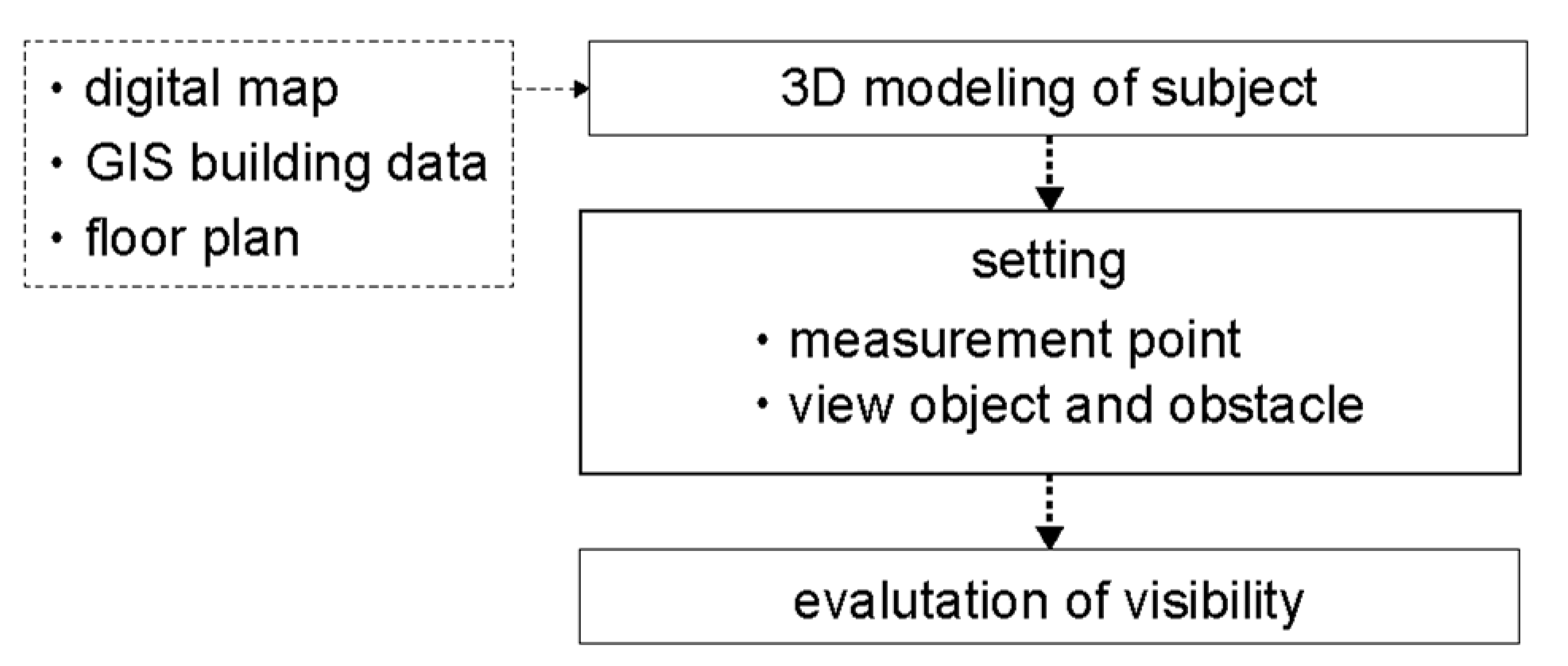
Figure 3.
Overview of ray radiated from a measurement point.
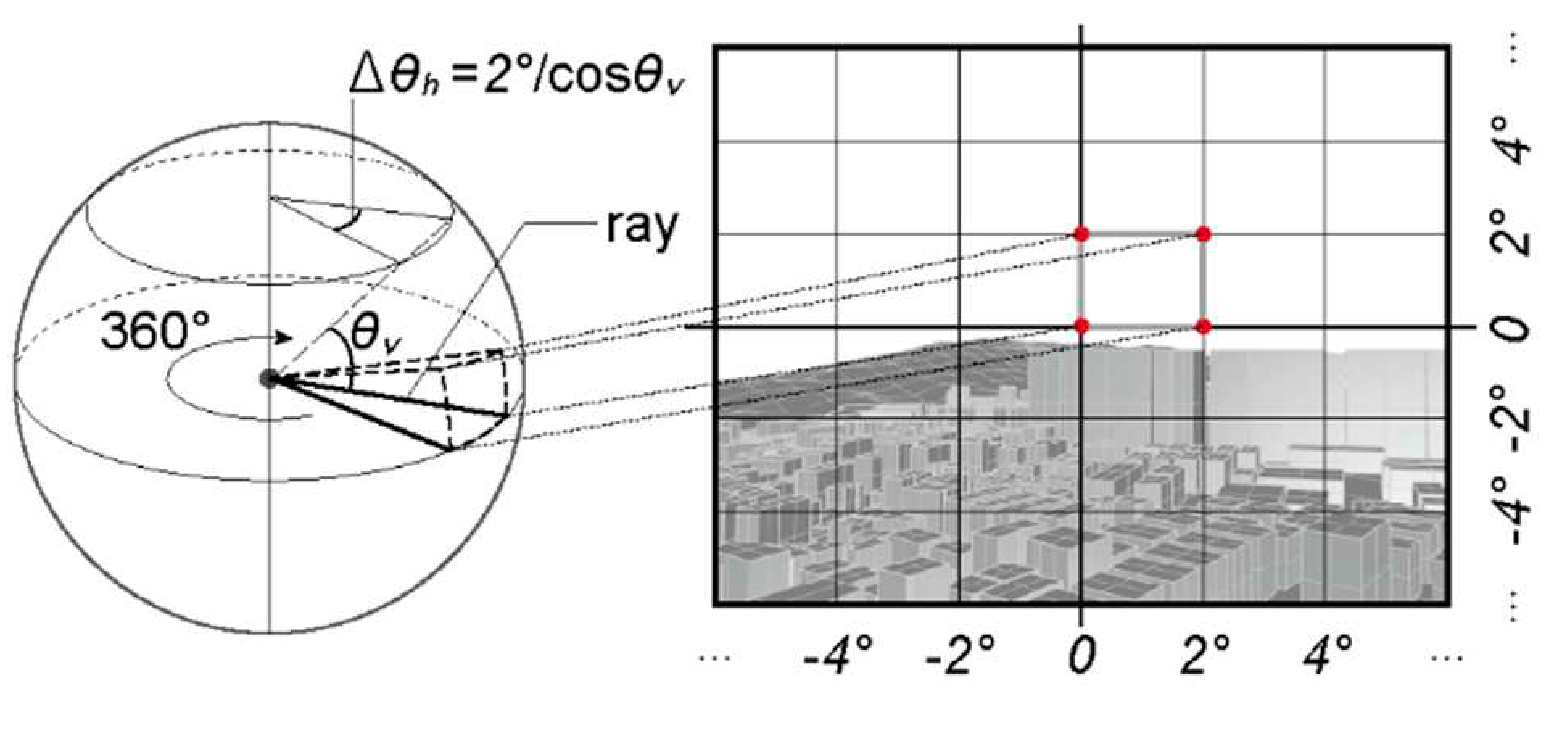
Figure 4.
Example of viewing based on window size with the same amount of visibility.
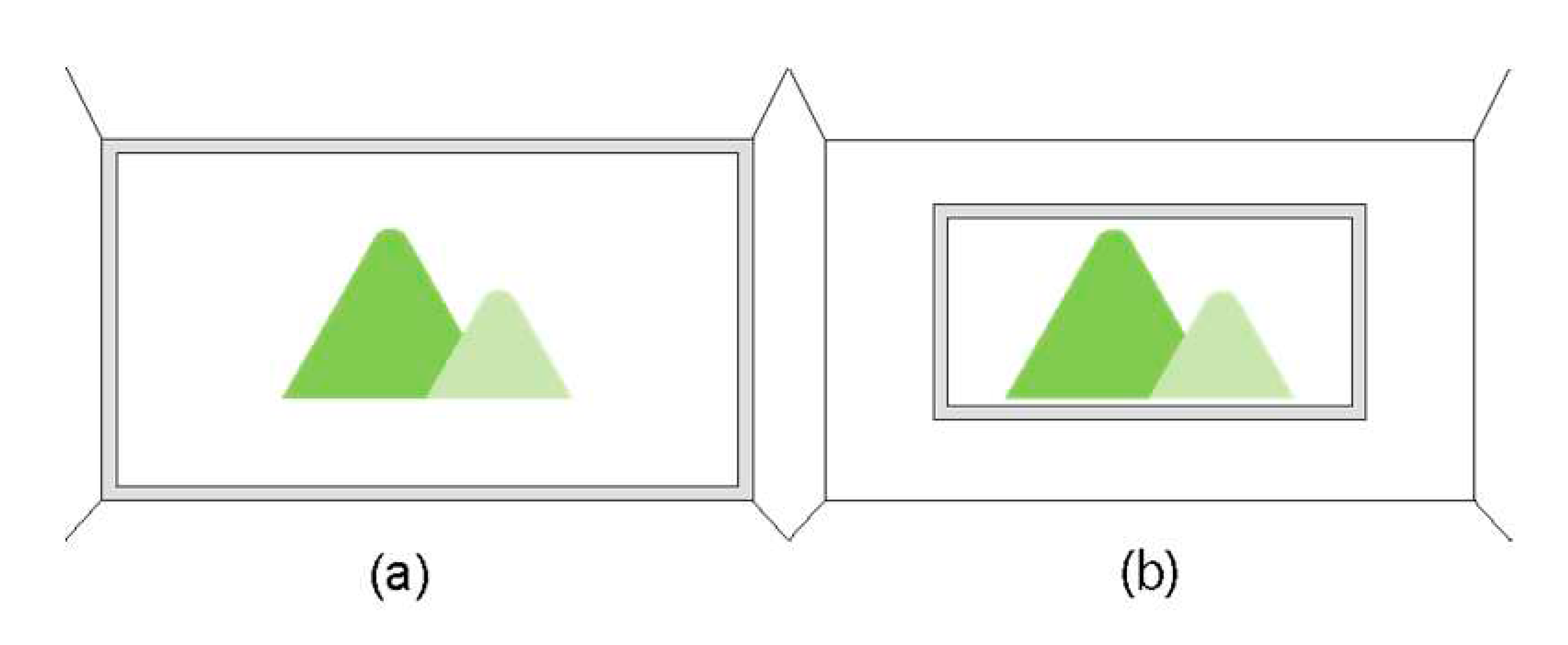
Figure 5.
Representatives of the room.
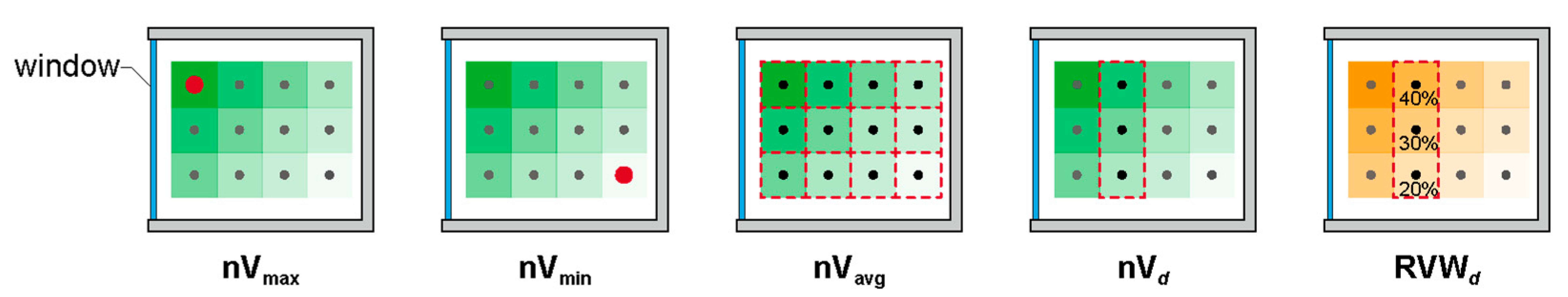
Figure 6.
Location of the object apartments and view objects.
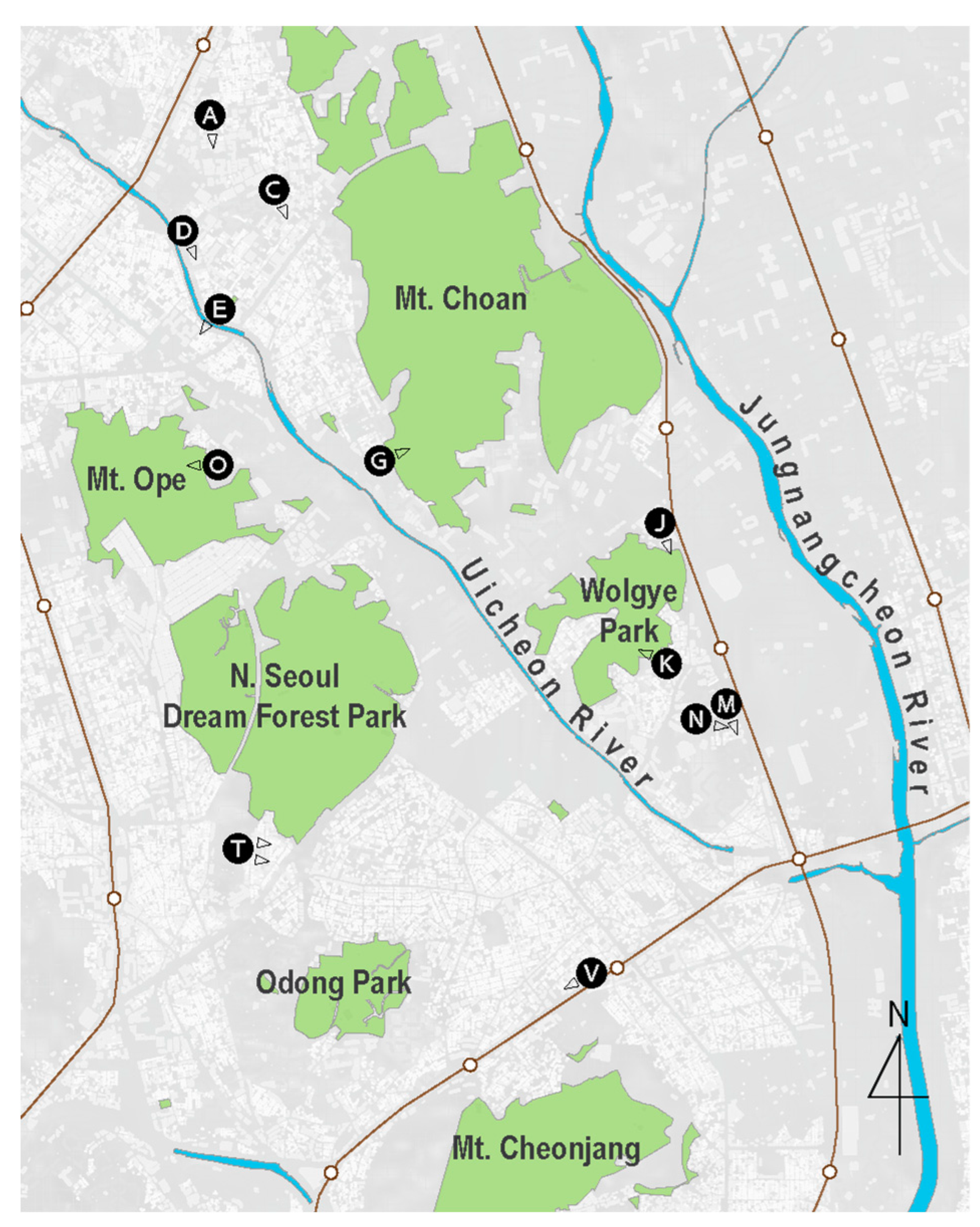
Figure 7.
Location of G2 and view object.
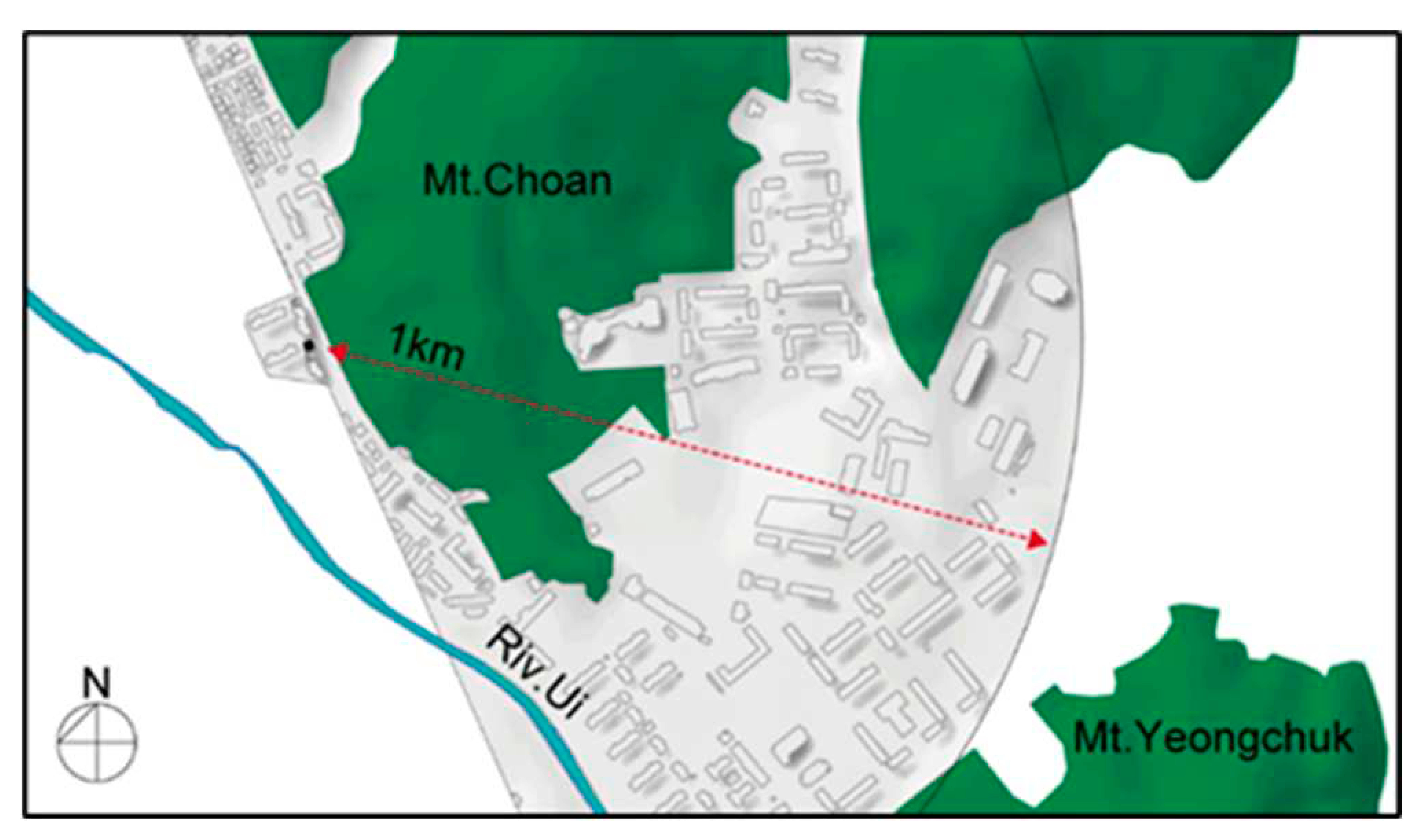
Figure 8.
Floor plan and living room of G2
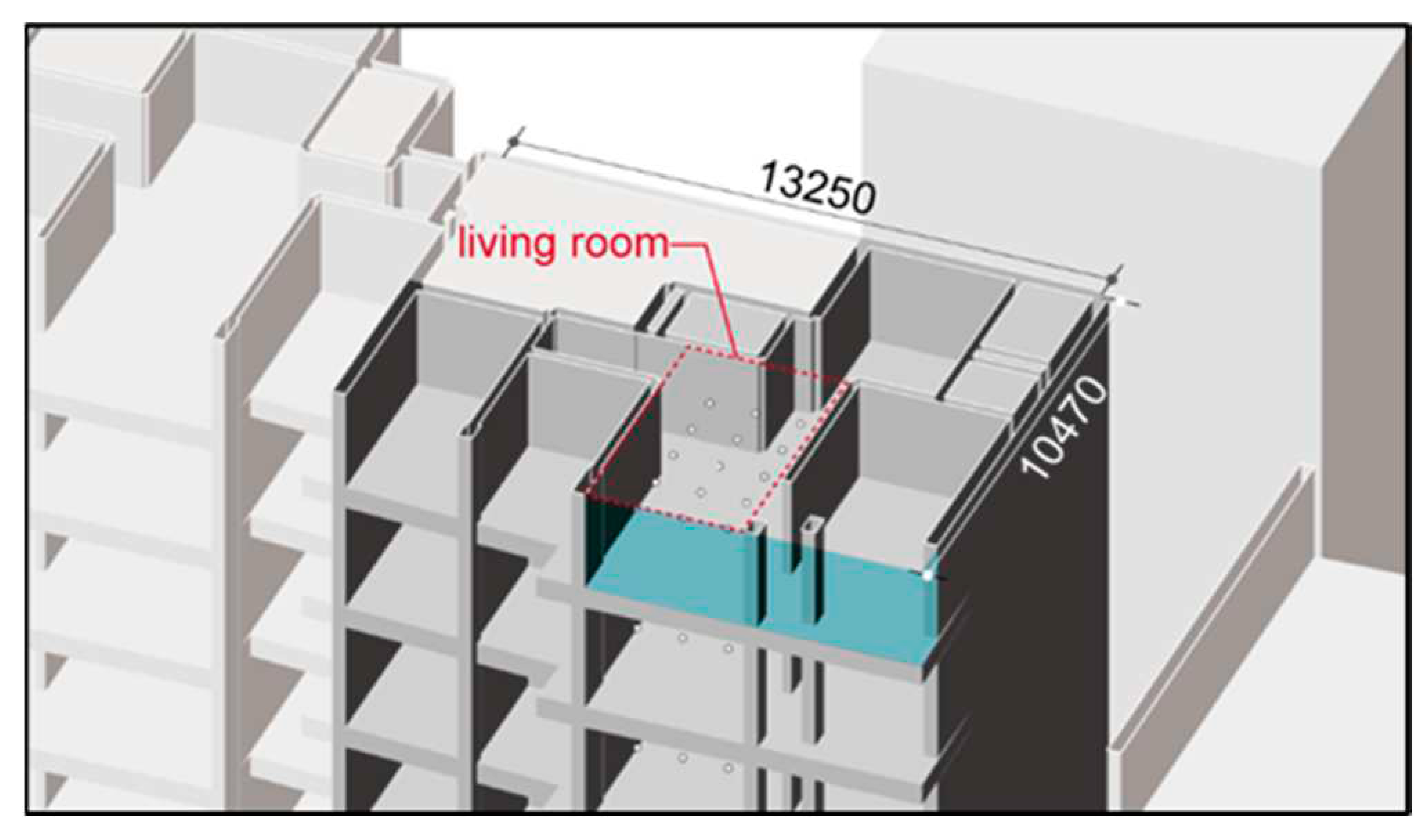
Figure 9.
Boxplot of nV of sky on each floor.
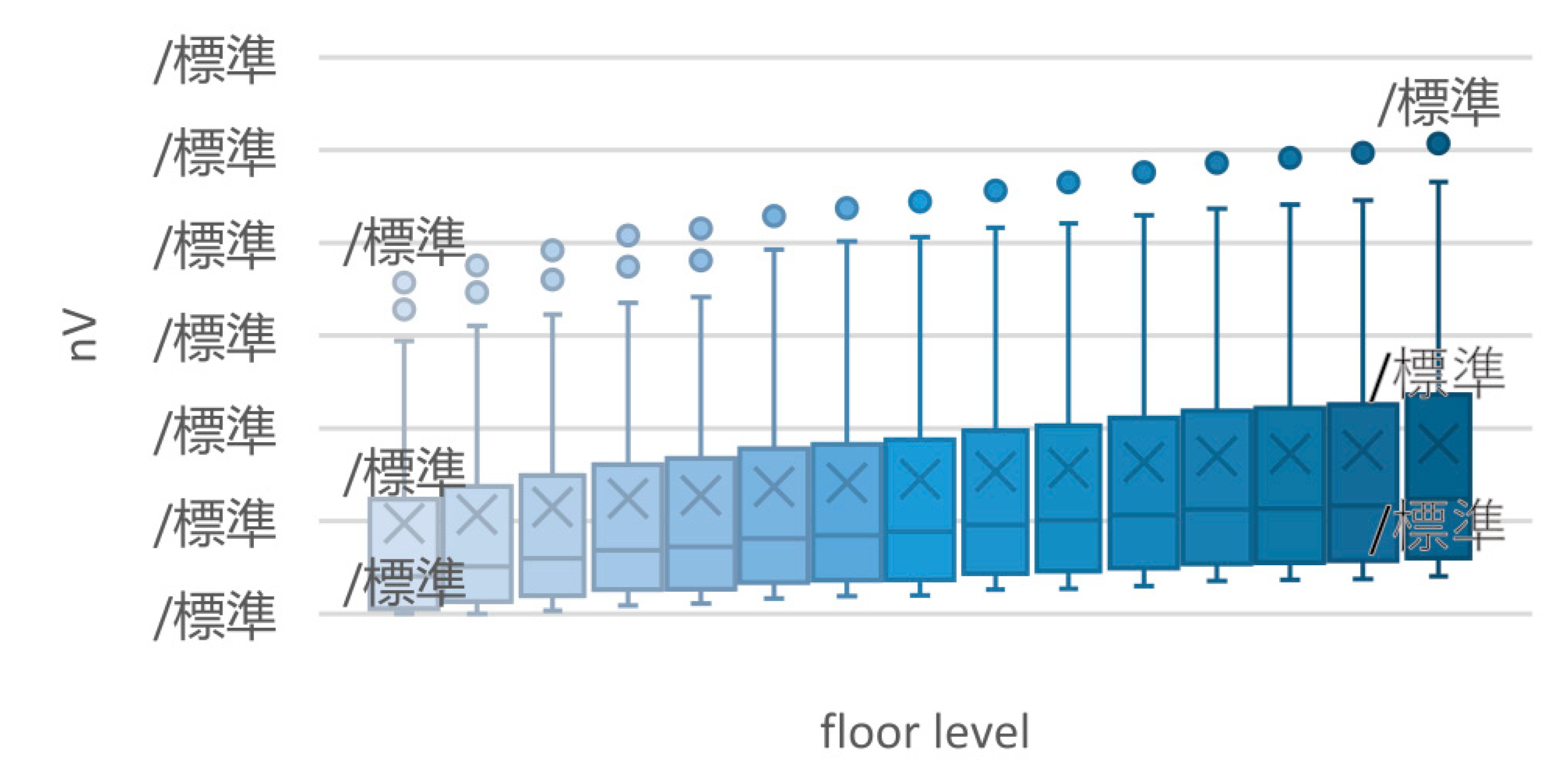
Figure 10.
Average of nV of sky depending on distance from window of each floor.
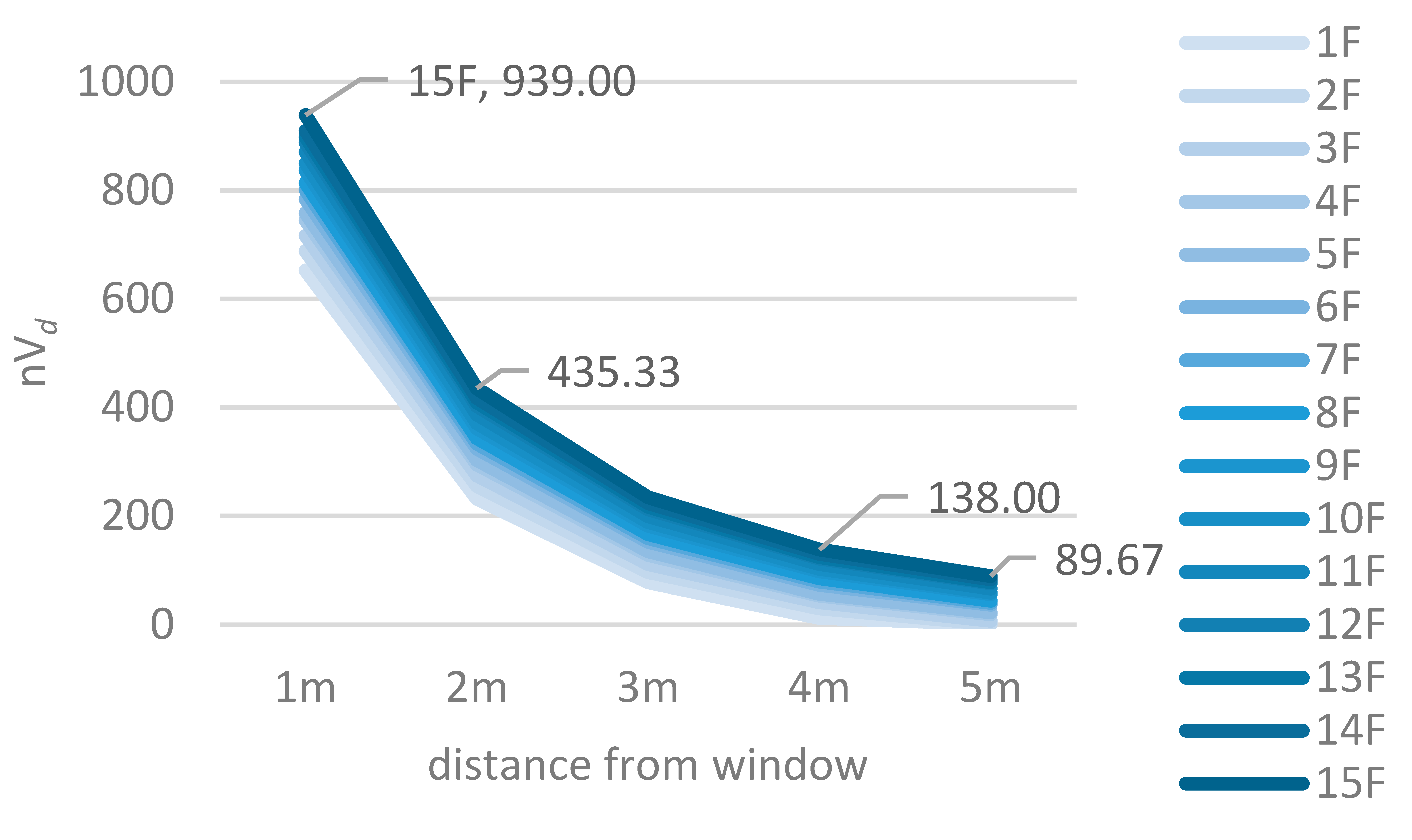
Figure 11.
Average of ratio of sky to window depending on distance from the window of each floor
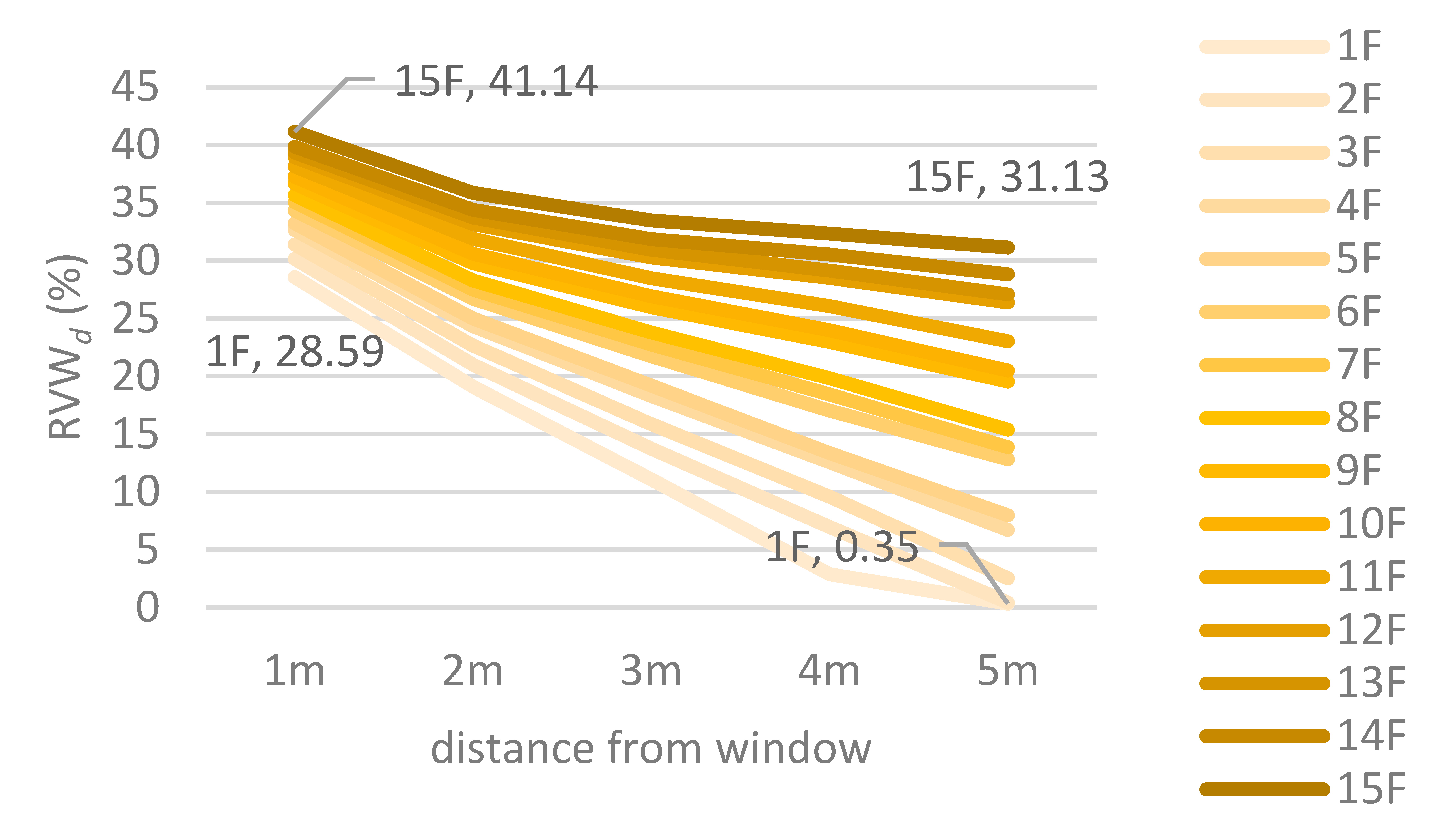
Figure 13.
Sum of nV of each natural object on each floor.
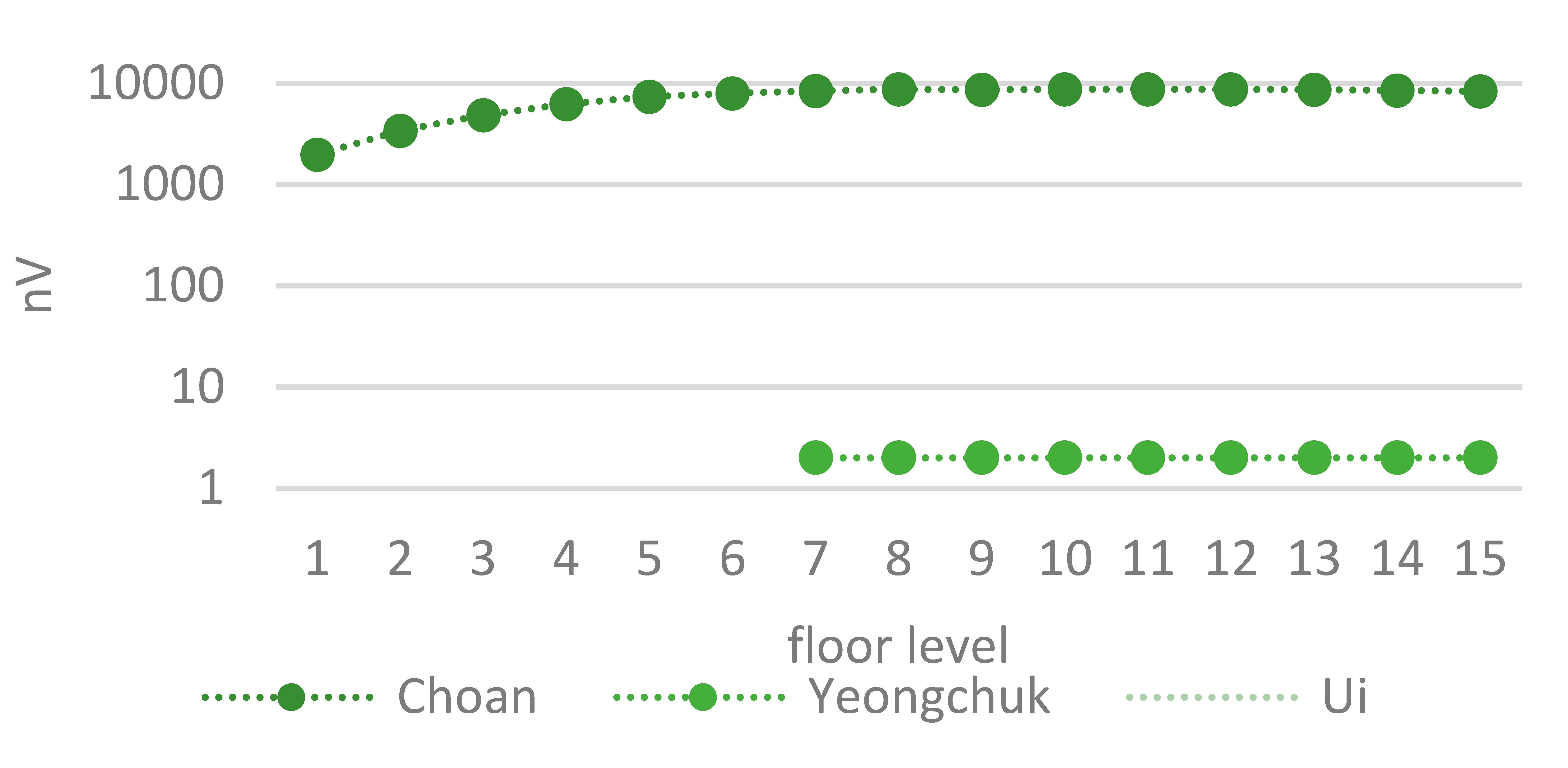
Figure 14.
Boxplot of the nV of natural object on each floor.
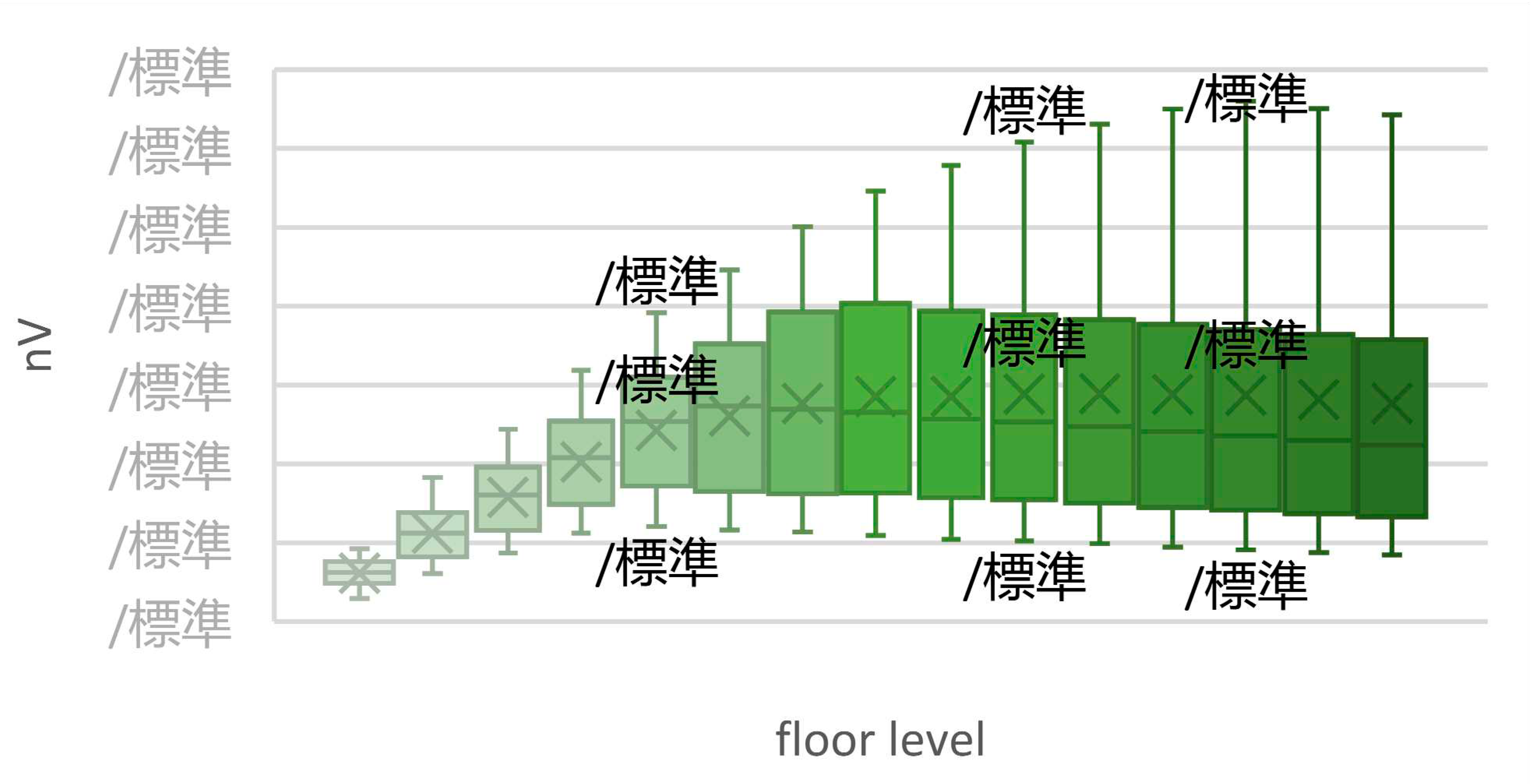
Figure 15.
Average of nV of natural object depending on distance from the window on each floor.
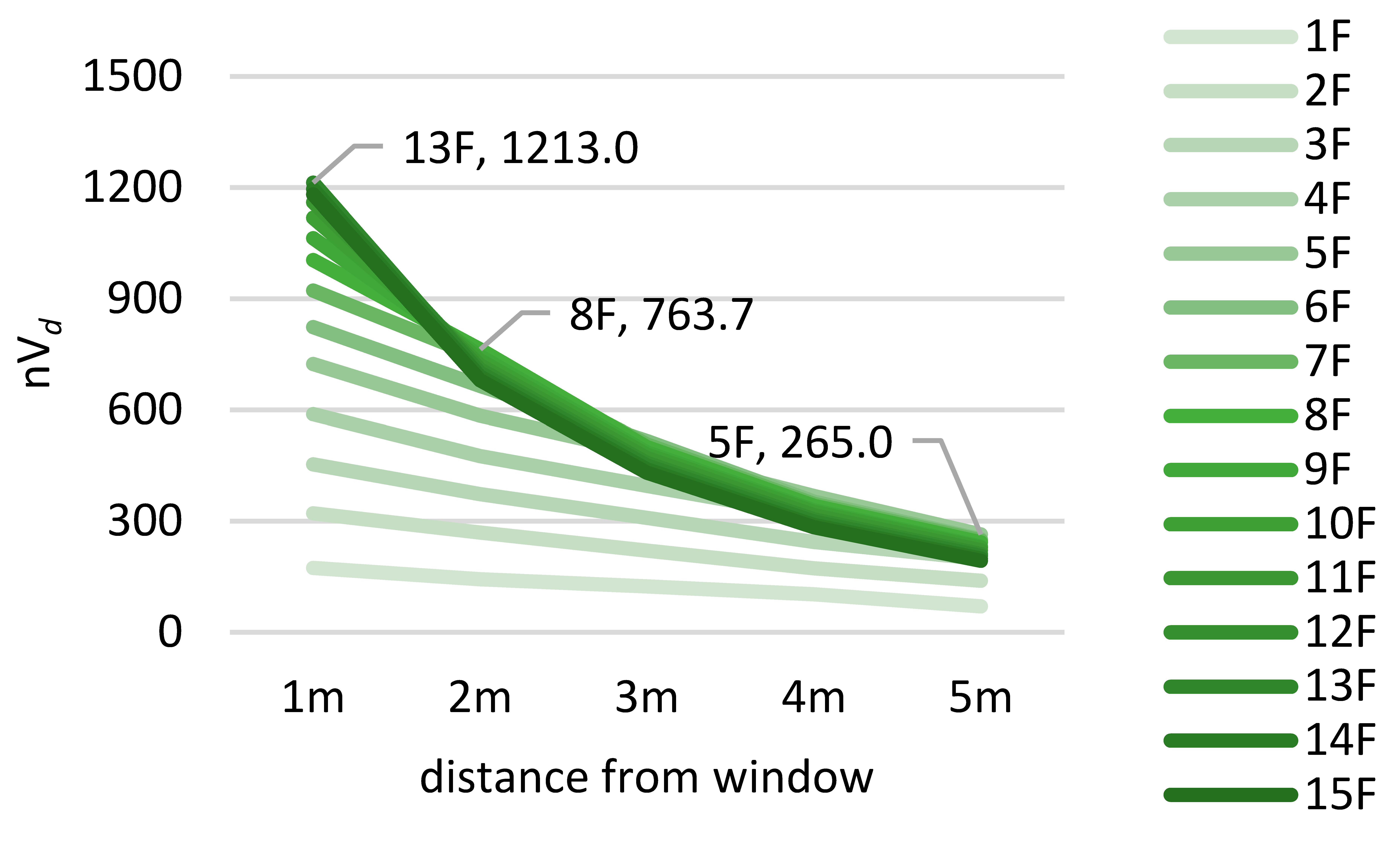
Figure 16.
Average of the ratio of natural object to the window depending on the distance from window.
Figure 16.
Average of the ratio of natural object to the window depending on the distance from window.
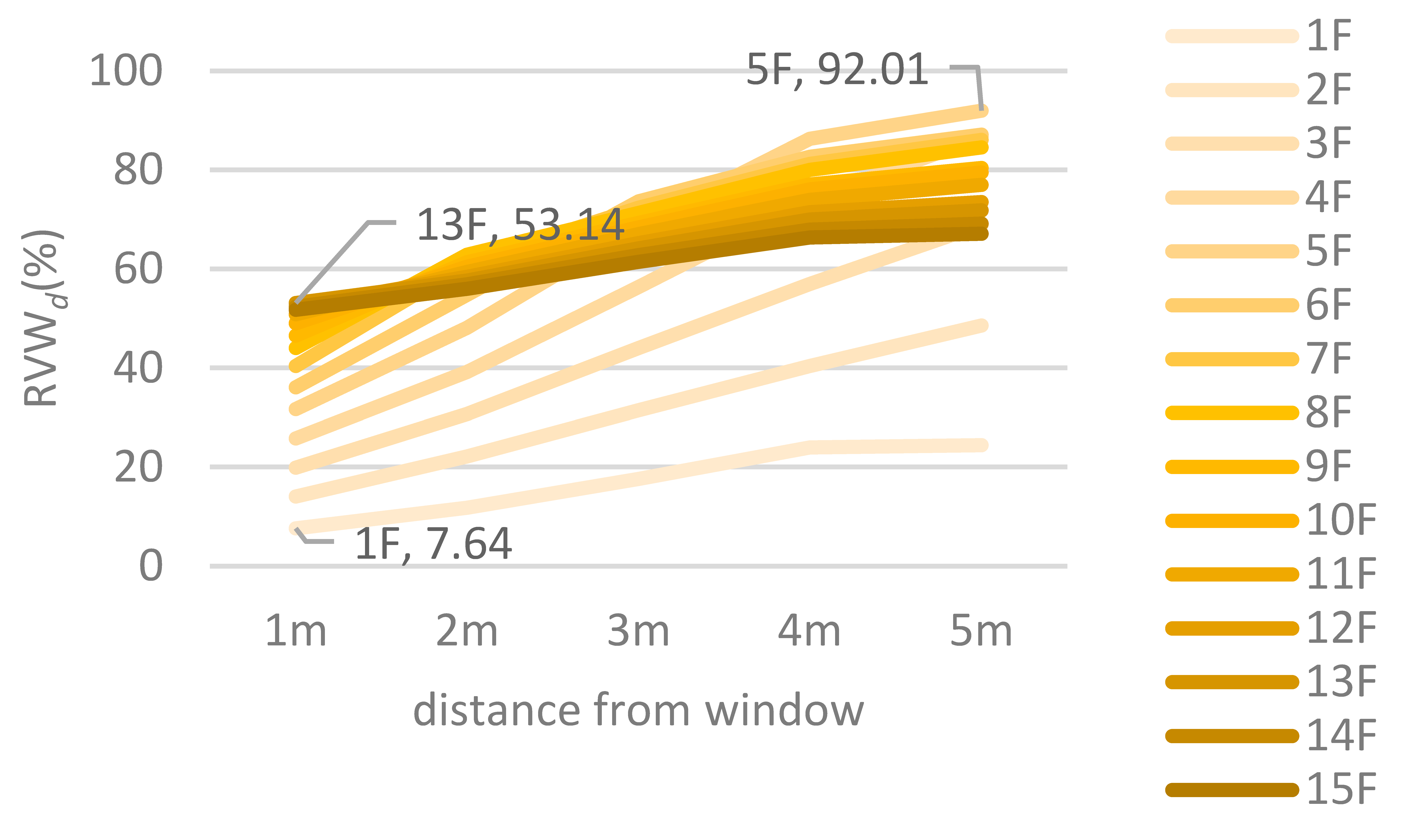
Figure 17.
Heatmap of nV and RVW of natural object of G2.
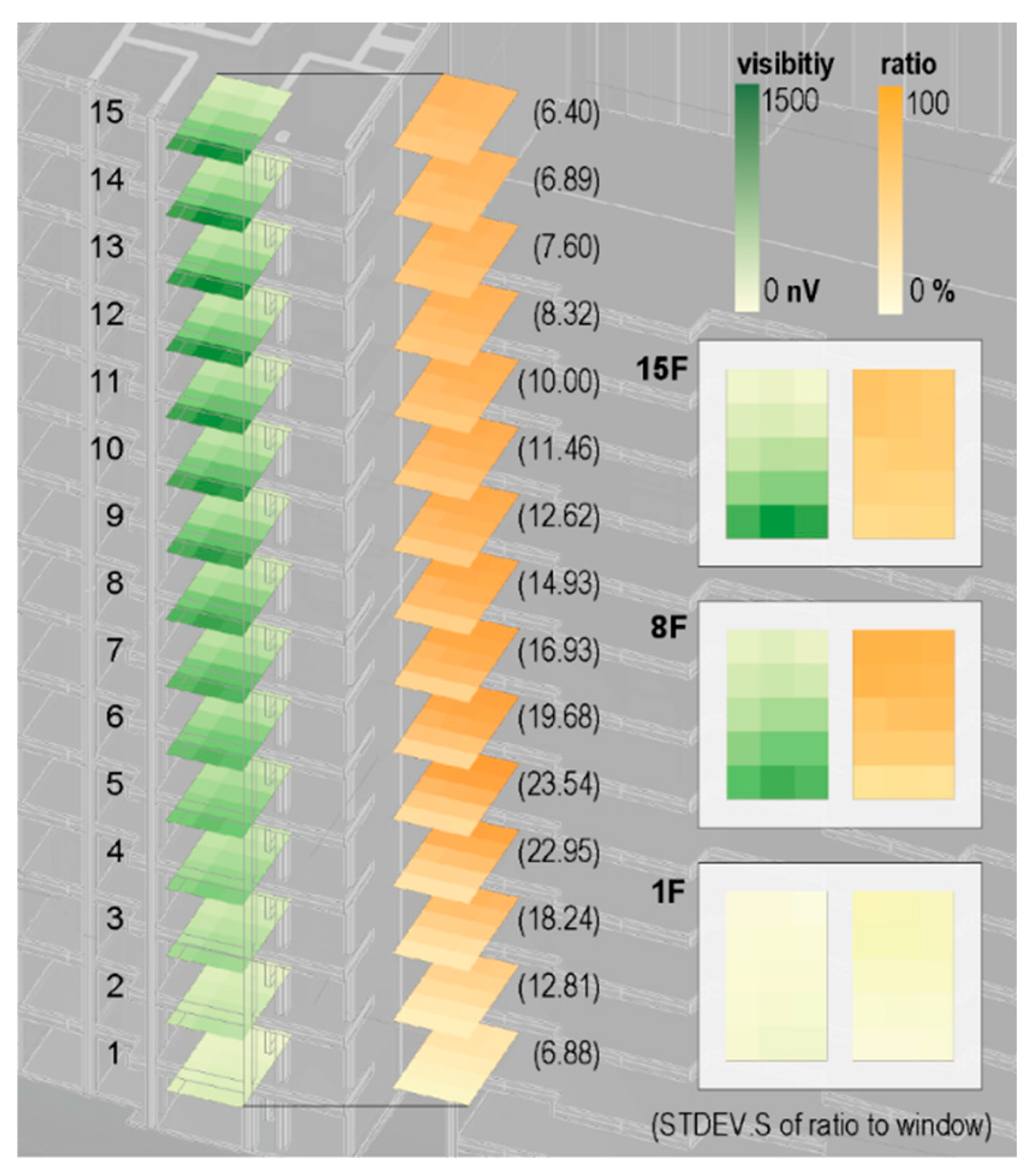

Table 1.
Location of the object apartments and view objects.
| CCD | EPA(m2) | Lowest fl. | Top fl. | House facing direction |
View Object | Number of measurement point |
|
|---|---|---|---|---|---|---|---|
| A | 2002 | 120.70 | 1 | 19 | S | Mt. Choan, Riv. Uicheon | 4×6 |
| C | 1995 | 59.71 | 1 | 19 | SE | Mt. Choan | 3×4 |
| D | 2002 | 56.38 | 3 | 18 | S | Mt. Choan, Mt. Ope, Riv.Uicheon | 3×6 |
| E1 | 1997 | 122.15 | 1 | 19 | SW | Mt. Ope, Riv. Uicheon | 3+4×5 |
| E2 | 1997 | 158.79 | 1 | 19 | SW | Mt. Ope, Riv. Uicheon | 4×6 |
| G1 | 2004 | 84.99 | 1 | 15 | EN | Mt. Choan, Riv. Uicheon, Mt. Yeongchuk | 4×6 |
| G2 | 2004 | 70.94 | 1 | 15 | EN | Mt. Choan, Riv. Uicheon | 3×5 |
| G3 | 2004 | 84.98 | 1 | 15 | EN | Mt. Choan, Riv. Uicheon | 4×6 |
| J2 | 2005 | 123.65 | 1 | 15 | S | Riv. Jungnang, Mt. Yeongchuk, Riv. Uicheon | 4×6 |
| K1 | 2005 | 84.96 | 3 | 15 | W | Riv. Uicheon | 4×5 |
| K2 | 2005 | 84.92 | 2 | 8 | N | Mt. Yeongchuk, Riv. Jungnangcheon | 4×6 |
| M | 2000 | 114.82 | 1 | 19 | S | Riv. Jungnang, Riv. Uicheon | 4×7 |
| N1 | 2005 | 64.18 | 3 | 15 | ES | Riv. Jungnang, Riv. Uicheon | 3×5 |
| O1 | 2001 | 117.97 | 1 | 18 | W | Dream forest, Mt. Ope, Riv. Uicheon | 4×6 |
| T1 | 2002 | 116.91 | 1 | 16 | E | Dream forest, Odong park | 4×6 |
| T2 | 2002 | 68.30 | 1 | 14 | SW | Dream forest, Odong park | 3×5 |
| V3 | 2001 | 41.41 | 3 | 6 | WS | Mt. Cheonjang, Odong park | 2+4×3 |
Table 2.
Summary of evaluations on each apartment unit.
| Number of transactions | Number of possible calculations runs |ta - tb| ≤ 6 (month) |
|
|---|---|---|
| A | 14 | 13 |
| C | 32 | 30 |
| D | 11 | 5 |
| E1 | 22 | 12 |
| E2 | 14 | 11 |
| G1 | 14 | 9 |
| G2 | 18 | 11 |
| G3 | 12 | 4 |
| J2 | 6 | 1 |
| K1 | 13 | 5 |
| K2 | 7 | 0 |
| M | 15 | 13 |
| N1 | 17 | 17 |
| O1 | 14 | 10 |
| T1 | 12 | 6 |
| T2 | 8 | 6 |
| V3 | 5 | 0 |
Table 3.
View value indicated by the floor representing the lowest, top floor, and largest of each apartment unit relative to the sky.
Table 3.
View value indicated by the floor representing the lowest, top floor, and largest of each apartment unit relative to the sky.
| Max | Avg | Min | standard deviation | |||||||||||||||||||
|---|---|---|---|---|---|---|---|---|---|---|---|---|---|---|---|---|---|---|---|---|---|---|
| top fl. | bottom fl. | largest | top fl. | bottom fl. | largest | top fl. | bottom fl. | largest | top fl. | bottom fl. | largest | |||||||||||
| nV | DW(m) | nV | DW(m) | nV | DW(m) | (Fl) | nV | nV | nV | (Fl) | nV | DW(m) | nV | DW(m) | nV | DW(m) | (Fl) | (Fl) | ||||
| RVW (%) | RVW (%) | RVW (%) | RVW (%) | RVW (%) | RVW (%) | RW (%) | RW (%) | RW (%) | RW (%) | RW (%) | RW (%) | |||||||||||
| A | 1240 | 1 | 637 | 1 | 〇 | (19) | 444.7 | 150.0 | 〇 | (19) | 108 | 6 | 2 | 6 | 〇 | (19) | ||||||
| 57.78 | 2 | 25.95 | 1 | 〇 | (19) | 49.46 | 16.69 | 〇 | (19) | 46.33 | 5 | 0.84 | 6 | 〇 | (19) | 2.38 | 9.08 | 10.13 | (2) | |||
| C | 1260 | 1 | 696 | 1 | 〇 | (19) | 582.8 | 255.3 | 〇 | (19) | 195 | 4 | 14 | 4 | 〇 | (19) | ||||||
| 47.92 | 4 | 27.87 | 1 | 〇 | (19) | 45.40 | 19.88 | 〇 | (19) | 42.48 | 4 | 3.05 | 4 | 〇 | (19) | 1.48 | 8.51 | 8.51 | (1) | |||
| D | 901 | 1 | 438 | 1 | 〇 | (18) | 334.0 | 133.7 | 〇 | (18) | 65 | 6 | 6 | 6 | 65 | 6 | (17,18) | |||||
| 53.39 | 5 | 20.62 | 1 | 〇 | (18) | 42.55 | 17.03 | 〇 | (18) | 35.46 | 5 | 3.37 | 6 | 〇 | (18) | 4.94 | 5.95 | 9.45 | (13) | |||
| E1 | 1445 | 1 | 1204 | 1 | 〇 | (19) | 487.8 | 348.0 | 〇 | (19) | 101 | 6 | 40 | 6 | 〇 | (19) | ||||||
| 43.43 | 2 | 34.63 | 1 | 〇 | (19) | 41.06 | 29.29 | 〇 | (19) | 37.27 | 6 | 14.93 | 6 | 〇 | (19) | 1.59 | 6.38 | 6.38 | (1) | |||
| E2 | 1257 | 1 | 1028 | 1 | 〇 | (19) | 474.5 | 332.5 | 〇 | (19) | 101 | 6 | 32 | 6 | 〇 | (19) | ||||||
| 43.94 | 1 | 35.93 | 1 | 〇 | (19) | 41.71 | 29.22 | 〇 | (19) | 37.55 | 6 | 11.81 | 6 | 〇 | (19) | 1.65 | 7.83 | 7.83 | (1) | |||
| G1 | 1004 | 1 | 476 | 1 | 〇 | (15) | 318.1 | 99.6 | 〇 | (15) | 52 | 6 | 0 | 5,6 | 〇 | (15) | ||||||
| 41.51 | 1 | 21.98 | 1 | 〇 | (15) | 34.67 | 10.85 | 〇 | (15) | 21.49 | 6 | 0.00 | 5,6 | 〇 | (15) | 5.75 | 6.51 | 9.39 | (5) | |||
| G2 | 1014 | 1 | 714 | 1 | 〇 | (15) | 367.3 | 195.1 | 〇 | (15) | 81 | 5 | 0 | 5 | 〇 | (15) | ||||||
| 41.40 | 1 | 29.17 | 1 | 〇 | (15) | 37.38 | 19.85 | 〇 | (15) | 28.62 | 5 | 0.00 | 5 | 〇 | (15) | 4.09 | 10.80 | 10.80 | (1) | |||
| G3 | 1059 | 1 | 777 | 1 | 〇 | (15) | 348.8 | 179.6 | 〇 | (15) | 59 | 6 | 0 | 5,6 | 〇 | (15) | ||||||
| 42.38 | 1 | 31.13 | 1 | 〇 | (15) | 38.02 | 19.57 | 〇 | (15) | 27.44 | 6 | 0.00 | 5,6 | 〇 | (15) | 3.96 | 11.32 | 11.62 | (2) | |||
| J2 | 1177 | 1 | 707 | 1 | 〇 | (15) | 405.0 | 172.1 | 〇 | (15) | 78 | 6 | 0 | 5,6 | 〇 | (15) | ||||||
| 43.89 | 1 | 28.60 | 1 | 〇 | (15) | 41.02 | 17.43 | 〇 | (15) | 31.58 | 6 | 0.00 | 5,6 | 〇 | (15) | 3.28 | 9.17 | 10.17 | (3) | |||
| K1 | 593 | 1 | 409 | 1 | 〇 | (15) | 244.1 | 160.2 | 〇 | (15) | 79 | 5 | 40 | 5 | 〇 | (15) | ||||||
| 38.51 | 5 | 21.43 | 5 | 〇 | (15) | 21.69 | 14.24 | 〇 | (15) | 16.52 | 1 | 11.25 | 4 | 〇 | (15) | 2.64 | 5.77 | 5.77 | (15) | |||
| K2 | 1082 | 1 | 963 | 1 | 〇 | (8) | 354.4 | 299.9 | 〇 | (8) | 73 | 6 | 52 | 6 | 73 | 6 | (7,8) | |||||
| 41.62 | 1 | 37.35 | 1 | 〇 | (8) | 38.68 | 32.73 | 〇 | (8) | 33.75 | 5 | 22.81 | 6 | 〇 | (8) | 2.20 | 3.96 | 3.96 | (2) | |||
| M | 913 | 1 | 369 | 1 | 〇 | (19) | 265.8 | 81.8 | 〇 | (19) | 17 | 7 | 0 | 5~7 | 〇 | (19) | ||||||
| 40.80 | 1 | 15.10 | 1 | 〇 | (19) | 32.84 | 10.10 | 〇 | (19) | 9.66 | 7 | 0.00 | 5~7 | 〇 | (19) | 7.71 | 4.49 | 9.13 | (18) | |||
| N1 | 1085 | 1 | 597 | 1 | 〇 | (15) | 370.5 | 194.6 | 〇 | (15) | 66 | 5 | 35 | 5 | 〇 | (15) | ||||||
| 38.72 | 1 | 21.93 | 1 | 〇 | (15) | 32.14 | 16.88 | 〇 | (15) | 18.54 | 4 | 9.68 | 4 | 〇 | (15) | 7.48 | 4.37 | 7.48 | (15) | |||
| O1 | 1213 | 1 | 790 | 1 | 〇 | (18) | 441.7 | 243.6 | 〇 | (18) | 87 | 6 | 14 | 6 | 〇 | (18) | ||||||
| 47.23 | 6 | 29.93 | 1 | 〇 | (18) | 42.58 | 23.49 | 〇 | (18) | 34.46 | 5 | 5.67 | 6 | 〇 | (18) | 3.36 | 6.07 | 6.97 | (4) | |||
| T1 | 1193 | 1 | 749 | 1 | 〇 | (16) | 444.4 | 213.3 | 〇 | (16) | 121 | 6 | 4 | 6 | 〇 | (16) | ||||||
| 53.63 | 6 | 28.48 | 1 | 53.63 | 6 | (15,16) | 43.27 | 20.76 | 〇 | (16) | 39.42 | 3 | 1.61 | 6 | 〇 | (16) | 7.56 | 4.35 | 7.56 | (1) | ||
| T2 | 1155 | 1 | 459 | 1 | 〇 | (14) | 466.1 | 98.5 | 〇 | (14) | 133 | 5 | 0 | 3,5 | 〇 | (14) | ||||||
| 48.43 | 5 | 18.11 | 1 | 〇 | (14) | 44.30 | 9.36 | 〇 | (14) | 40.64 | 4 | 0.00 | 3,5 | 〇 | (14) | 2.00 | 6.62 | 10.16 | (3) | |||
| V3 | 678 | 1 | 659 | 1 | 678 | (6) | 232.4 | 220.7 | 〇 | (6) | 49 | 4 | 39 | 4 | 〇 | (6) | ||||||
| 34.99 | 2 | 34.00 | 2 | 〇 | 2 | (5,6) | 26.54 | 25.21 | 〇 | (6) | 14.66 | 2 | 12.79 | 4 | 〇 | (6) | 6.35 | 6.73 | 6.73 | (3) | ||
DW: Distance from window, 〇: Top floor represents the largest value.
Table 4.
View value indicated by the floor representing the lowest, top floor, and largest of each apartment unit relative to the natural objects.
Table 4.
View value indicated by the floor representing the lowest, top floor, and largest of each apartment unit relative to the natural objects.
| Max | Avg | Min | standard deviation | |||||||||||||||||||
|---|---|---|---|---|---|---|---|---|---|---|---|---|---|---|---|---|---|---|---|---|---|---|
| top fl. | bottom fl. | largest | top fl. | bottom fl. | largest | top fl. | bottom fl. | largest | top fl. | bottom fl. | largest | |||||||||||
| nV | DW(m) | nV | DW(m) | nV | DW(m) | (Fl) | nV | nV | nV | (Fl) | nV | DW(m) | nV | DW(m) | nV | DW(m) | (Fl) | (Fl) | ||||
| RVW (%) | RVW (%) | RVW (%) | RVW (%) | RVW (%) | RVW (%) | RW (%) | RW (%) | RW (%) | RW (%) | RW (%) | RW (%) | |||||||||||
| A | 34 | 1 | 0 | A | 〇 | (19) | 13.0 | 0.0 | 〇 | (19) | 0 | 3~6 | 0 | A | 0 | (1) | ||||||
| 3.65 | 4 | 0.00 | A | 〇 | (19) | 1.45 | 0.00 | 〇 | (19) | 0.00 | 3~6 | 0.00 | A | 0.00 | (1) | 1.11 | 0.00 | 1.11 | (19) | |||
| C | 87 | 1 | 0 | A | 〇 | (19) | 52.1 | 0.0 | 〇 | (19) | 13 | 4 | 0 | A | 13 | (19) | ||||||
| 7.78 | 3 | 0.00 | A | 〇 | (19) | 4.06 | 0.00 | 〇 | (19) | 2.75 | 3 | 0.00 | A | 2.75 | (19) | 1.70 | 0.00 | 1.70 | (19) | |||
| D | 39 | 1 | 0 | A | 〇 | (18) | 16.2 | 0.0 | 〇 | (18) | 1 | 6 | 0 | 2 | 6 | (17) | ||||||
| 4.08 | 4 | 0.00 | A | 〇 | (18) | 2.06 | 0.00 | 〇 | (18) | 0.55 | 6 | 0.00 | 1.10 | 6 | (17) | 0.92 | 0.00 | 0.92 | (18) | |||
| E1 | 254 | 1 | 85 | 1 | 287 | 1 | (15) | 70.7 | 51.9 | 105.6 | (5) | 27 | 6 | 25 | 6 | 33 | 6 | (2) | ||||
| 15.54 | 6 | 9.96 | 6 | 18.45 | 6 | (2) | 5.95 | 4.37 | 8.89 | (5) | 2.57 | 2 | 2.29 | 1 | 5.40 | 1 | (5) | 3.70 | 2.53 | 4.49 | (2) | |
| E2 | 188 | 1 | 75 | 1 | 245 | 1 | (10) | 67.0 | 48.8 | 97.9 | (5) | 22 | 6 | 23 | 6 | 37 | 5 | (3) | ||||
| 17.10 | 6 | 11.15 | 6 | 19.56 | 6 | (3) | 5.89 | 4.29 | 8.61 | (5) | 2.75 | 2 | 2.59 | 1 | 4.68 | 6 | (5) | 3.70 | 2.55 | 4.25 | (3) | |
| G1 | 1089 | 1 | 230 | 1 | 1097 | 1 | (14) | 441.6 | 130.8 | 467.4 | (11) | 151 | 6 | 45 | 6 | 180 | 6 | (8) | ||||
| 71.60 | 6 | 41.74 | 6 | 91.36 | 6 | (8) | 48.14 | 14.26 | 50.94 | (11) | 36.77 | 1 | 7.22 | 1 | 37.10 | 1 | (14) | 10.40 | 9.93 | 17.18 | (8) | |
| G2 | 1285 | 1 | 185 | 1 | 1320 | 1 | (13) | 553.9 | 122.7 | 577.9 | (11) | 169 | 5 | 59 | 5 | 241 | 5 | (5) | ||||
| 69.96 | 5 | 25.80 | 5 | 92.72 | 5 | (5) | 56.36 | 12.49 | 58.81 | (11) | 50.26 | 1 | 7.41 | 1 | 51.56 | 1 | (13) | 6.40 | 6.88 | 23.54 | (5) | |
| G3 | 1366 | 1 | 180 | 1 | 1367 | 1 | (14) | 520.0 | 109.5 | 540.5 | (10) | 148 | 6 | 42 | 6 | 212 | 6 | (5) | ||||
| 71.63 | 6 | 22.87 | 5 | 98.60 | 6 | (5) | 56.69 | 11.94 | 58.92 | (10) | 50.23 | 1 | 6.62 | 1 | 50.83 | 1 | (14) | 5.98 | 5.51 | 25.35 | (5) | |
| J2 | 490 | 1 | 61 | 1 | 〇 | (15) | 273.8 | 30.2 | 〇 | (15) | 52 | 6 | 1 | 4~6 | 68 | 6 | (12) | |||||
| 58.88 | 5 | 7.99 | 4 | 65.99 | 6 | (11) | 27.73 | 3.06 | 〇 | (15) | 13.74 | 1 | 0.22 | 4 | 13.74 | 1 | (15) | 13.75 | 2.31 | 15.80 | (12) | |
| K1 | 0 | 0 | 1 | 1,2 | (14) | 0.0 | 0.0 | 0.3 | (14) | 0 | 0 | 0 | (1~15) | |||||||||
| 0.00 | 0.00 | 0.07 | 2 | (14) | 0.00 | 0.00 | 0.03 | (14) | 0.00 | 0.00 | 0.00 | (1~15) | 0.00 | 0.00 | 0.02 | (14) | ||||||
| K2 | 459 | 1 | 316 | 1 | 〇 | 1 | (8) | 153.8 | 123.6 | 156.0 | (7) | 0 | 5~6 | 0 | 4~6 | 0 | (1~8) | |||||
| 29.11 | 2 | 25.62 | 3 | 31.88 | 3 | (6) | 16.78 | 13.49 | 17.02 | (7) | 0.00 | 5~6 | 0.00 | 4~6 | 0.00 | (1~8) | 9.39 | 8.21 | 9.91 | (6) | ||
| M | 0 | 0 | 0 | 0.0 | 0.0 | 0.0 | 0 | 0 | 0 | |||||||||||||
| 0.00 | 0.00 | 0.00 | 0.00 | 0.00 | 0.00 | 0.00 | 0.00 | 0.00 | 0.00 | 0.00 | 0.00 | |||||||||||
| N1 | 0 | 0 | 3 | 1~4 | (12) | 0.0 | 0.0 | 1.2 | (12) | 0 | 0 | 0 | (3) | |||||||||
| 0.00 | 0.00 | 0.62 | 4 | (12) | 0.00 | 0.00 | 0.10 | (12) | 0.00 | 0.00 | 0.00 | (3) | 0.00 | 0.00 | 0.18 | (12) | ||||||
| O1 | 1124 | 1 | 128 | 1 | 1124 | 1 | (17) | 444.7 | 75.3 | 460.3 | (11) | 103 | 6 | 37 | 5,6 | 153 | 6 | (4) | ||||
| 64.97 | 5 | 24.29 | 6 | 87.45 | 6 | (5) | 42.87 | 7.26 | 44.38 | (11) | 34.69 | 3 | 3.34 | 1 | 36.99 | 3 | (12) | 9.26 | 6.04 | 21.73 | (4) | |
| T1 | 118 | 1 | 38 | 1 | 〇 | (16) | 18.8 | 3.0 | 〇 | (16) | 2 | 6 | 0 | 1~6 | 2 | (16) | ||||||
| 4.21 | 1 | 1.36 | 1 | 〇 | (16) | 1.83 | 0.29 | 〇 | (16) | 0.24 | 2 | 0.00 | 1~6 | 0.36 | 6 | (13) | 1.01 | 0.32 | 1.01 | (16) | ||
| T2 | 12 | 1 | 0 | 5 | 12 | (14) | 3.8 | 0.0 | 4.0 | (13) | 0 | 5 | 0 | 1 | 5 | (11) | ||||||
| 1.29 | 5 | 0.00 | 5 | 1.29 | 5 | (13) | 0.36 | 0.00 | 0.38 | (13) | 0.00 | 5 | 0.00 | 0.12 | 1 | (11) | 0.32 | 0.00 | 0.34 | (13) | ||
| V3 | 4 | 1~4 | 2 | 1~4 | 〇 | (6) | 2.4 | 1.2 | 〇 | (6) | 0 | 2~4 | 0 | 2~4 | 0 | 2~4 | (3) | |||||
| 1.19 | 4 | 0.59 | 4 | 〇 | (6) | 0.28 | 0.14 | 〇 | (6) | 0.00 | 2~4 | 0.00 | 2~4 | 0.00 | 2~4 | (3) | 0.36 | 0.18 | 0.36 | (6) | ||
DW: Distance from window, 〇: Top floor represents the largest value
Table 5.
Correlation coefficient of floor and view visibility with the real transaction price.
| sky | Natural object | Floor | |||
|---|---|---|---|---|---|
| Rmax | Ravg | Rmax | Ravg | Rfl | |
| A | 0.8945* | 0.9016* | 0.8285* | 0.8525* | 0.9408* |
| C | 0.0820 | 0.1299 | 0.0865 | 0.0745 | 0.1054 |
| E1 | -0.2269 | -0.2134 | -0.0236 | 0.2513 | -0.2782 |
| E2 | -0.0880 | -0.0789 | -0.0787 | 0.0307 | -0.0754 |
| G2 | 0.6002 | 0.5873 | 0.8217* | 0.7722* | 0.5250 |
| M | 0.7015* | 0.6711* | ― | ― | 0.7391* |
| N1 | 0.1170 | 0.0496 | 0.9842 | 0.9782 | 0.1312 |
| O1 | 0.7373* | 0.7250* | 0.7867* | 0.7337* | 0.7007* |
* p-value < 0.05.
Table 6.
Summary of evaluations on each apartment unit.
| A | C | D | E1 | E2 | G1 | G2 | G3 | J2 | K1 | K2 | M | N1 | O1 | T1 | T2 | V3 | |||
| Sky | Visible quantity | It is visible on all floors | 〇 | 〇 | 〇 | 〇 | 〇 | 〇 | 〇 | 〇 | 〇 | 〇 | 〇 | 〇 | 〇 | 〇 | 〇 | 〇 | 〇 |
| It is visible even at the far end of the room on all floors. | 〇 | 〇 | 〇 | 〇 | 〇 | 〇 | 〇 | 〇 | 〇 | 〇 | 〇 | ||||||||
| Most visible floor is the top floor. | 〇 | 〇 | 〇 | 〇 | 〇 | 〇 | 〇 | 〇 | 〇 | 〇 | 〇 | 〇 | 〇 | 〇 | 〇 | 〇 | 〇 | ||
| The floor of the unit most visible at the window is same as that of the unit most visible in the entire room. | 〇 | 〇 | 〇 | 〇 | 〇 | 〇 | 〇 | 〇 | 〇 | 〇 | 〇 | 〇 | 〇 | 〇 | 〇 | 〇 | 〇 | ||
| The ratio to the window area | The widest perception in proportion to the window is on the window side. | 〇 | 〇 | 〇 | 〇 | 〇 | 〇 | 〇 | 〇 | ||||||||||
| It is visible over a larger area as one moves toward the back of the room relative to the window. | |||||||||||||||||||
| The unit with the smallest variation in visible amount relative to the entire room is on the lower floors. (less than 5) | 〇 | 〇 | 〇 | 〇 | 〇 | 〇 | 〇 | 〇 | 〇 | 〇 | 〇 | 〇 | 〇 | ||||||
| The unit with the smallest variation in visible amount relative to the entire room is on the higher floors. (more than 10) | 〇 | 〇 | 〇 | 〇 | |||||||||||||||
| Natural objects | Visible quantity | It is visible on all floors. | 〇 | 〇 | 〇 | 〇 | 〇 | 〇 | 〇 | 〇 | 〇 | 〇 | |||||||
| It is visible even at the far end of the room on all floors. | 〇 | 〇 | 〇 | 〇 | 〇 | 〇 | 〇 | ||||||||||||
| Most visible floor is the top floor. | 〇 | 〇 | 〇 | 〇 | 〇 | 〇 | 〇 | 〇 | |||||||||||
| It is rarely visible.(nV of all measurement points is less than 15) | 〇 | 〇 | 〇 | 〇 | 〇 | ||||||||||||||
| The floor of the unit most visible at the window is same as that of the unit most visible in the entire room. | 〇 | 〇 | 〇 | 〇 | 〇 | 〇 | 〇 | 〇 | |||||||||||
| The floor of the unit most visible at the window is higher than that of the unit most visible throughout the room. | 〇 | 〇 | 〇 | 〇 | 〇 | 〇 | 〇 | 〇 | |||||||||||
| The ratio to the window area | The widest perception in proportion to the window is on the window side. | 〇 | |||||||||||||||||
| The unit with the smallest variation in visible amount relative to the entire room is on the lower floors. (less than 5) | 〇 | 〇 | 〇 | 〇 | 〇 | ||||||||||||||
| The unit with the smallest variation in visible amount relative to the entire room is on the higher floors. (more than 10) | 〇 | 〇 | 〇 | 〇 | 〇 | 〇 | 〇 | 〇 |
Disclaimer/Publisher’s Note: The statements, opinions and data contained in all publications are solely those of the individual author(s) and contributor(s) and not of MDPI and/or the editor(s). MDPI and/or the editor(s) disclaim responsibility for any injury to people or property resulting from any ideas, methods, instructions or products referred to in the content. |
© 2023 by the authors. Licensee MDPI, Basel, Switzerland. This article is an open access article distributed under the terms and conditions of the Creative Commons Attribution (CC BY) license (http://creativecommons.org/licenses/by/4.0/).
Copyright: This open access article is published under a Creative Commons CC BY 4.0 license, which permit the free download, distribution, and reuse, provided that the author and preprint are cited in any reuse.


