
Submitted:
24 August 2023
Posted:
24 August 2023
You are already at the latest version
Abstract
The advancement of technology and the availability of specialized digital signal processing chips have made digital filter design and implementation more feasible in a variety of fields, including biomedical engineering. This paper makes two key contributions. First, it uses a genetic algorithm to optimize the coefficients of Finite Impulse Response (FIR) filters. Second, it conducts a case study on using genetic algorithms to optimize FIR filters for electrocardiogram (ECG) biomedical signal noise removal. The goal of the proposed filter design approach is to achieve the desired signal bandwidth while minimizing the side lobe level and eliminating unwanted signals using a genetic algorithm. The results of the comprehensive analysis of the impact of different genetic operators show that the genetic algorithm-based filter outperforms conventional filter designs.
Keywords:
Genetic Algorithms
; Digital Filters
; Metaheuristic Optimization
; Finite Impulse Response (FIR)
; Side Lobe Level (SLL).
1. Introduction
Digital filters are used in many different fields to remove noise, split multiple signals [1], missing data imputation [2], and enhance the quality of received signals [3,4]. In recent years, there has been a lot of research into the use of Genetic Algorithms to optimize the design of digital filters. A Genetic algorithm [5] is a metaheuristic optimization algorithm that can be used to find optimal, or near optimal, solutions to problems that are too computationally expensive and are difficult to solve using traditional methods. In the case of digital filter optimization, the goal is to find a set of coefficients that optimizes the performance of the filter using some performance metric.
Electrocardiography (ECG) is a well-known and reliable tool that is widely used in the medical field to analyze and diagnose the condition of the heart. This analysis is very crucial for the early detection of heart diseases. ECG signals are very weak signals and hence susceptible to disturbances in the measurement environment. Using digital filters to remove unwanted parts of these signals is very critical for the performance and accuracy of the algorithms and software tools that are used to detect abnormal heart conditions [6].
The side lobe level (SLL) [7] is a measure of the noise that is produced by the filter outside of its passband. A low side lobe level indicates that the filter is good at removing noise. The genetic algorithm works by iteratively generating new populations of filters, each of which is a slight variation of the previous population. The filters in each population are evaluated based on their side lobe level, and the best filters are selected to create the next generation. This process continues until a filter with a sufficiently low side lobe level is found.
The genetic algorithm approach to digital filter optimization has several advantages over traditional methods [8,9]. First, it is not limited to finding local minima, which can be a problem with traditional methods. Second, it can be used to find solutions to problems that are too complex for traditional methods. Third, it is relatively easy to implement. This approach is a promising technique that has the potential to significantly enhance the design of digital filters used in different fields, including biomedical engineering.
In this paper, a GA-based digital filter is proposed to optimize the coefficients of FIR filters for ECG signals. The search space for the filter is defined by 20 coefficients. Finding the optimal values of these coefficients is practically extremely large due to the high non-linearity of the frequency response of the filters. The objective, or fitness, function to be optimized is the minimization of the side lobe level (). As discussed earlier in this section, the is a measure of the noise that is produced by the filter outside of its passband. A low indicates that the filter is good at removing noise. The actual coefficients of the filter are mapped to the genes of a chromosome. Each coefficient represents a gene, while the whole coefficients represent a chromosome. The genetic algorithm works by iteratively generating new populations of filters, each of which is a slight variation of the previous population. The filters in each population are evaluated based on their SLL, and the best filters are selected to create the next generation. This process continues until a filter with a sufficiently low SLL is found.
The remainder of the paper is organized as follows. Section 2 presents the related work. Section 3 explain the research methodology. Section 4 highlight and compare different options of the proposed methodology. At the same time, Section 5 discuss the results for the case study of using to filter ECG signal. Eventually, Section 6 concludes the paper.
2. RELATED WORK
Meta-heuristic optimization algorithms such as Genetic Algorithms () [10], Ant Colony Optimization () [11], and Chemical Reaction Optimization () [12] are used to solve different optimization problems. These algorithms have been extensively used in recent years to implement digital filters in a wide range of applications [13].
The authors in [14] proposed a comprehensive fitness function for an infinite impulse response () digital filter design with six terms, including a low delay parameter. Low delay filters are preferred since they achieve quasi-real-time processing. Other parameters can be included in the fitness function to meet linear phase, minimum phase and stability constraints.
The authors in [15] proposed a method to detect breast malignancies. The filter bank that has been used to obtain the filter response is the Maximum Response Eight Filter Bank. Genetic Algorithm and Linear Discriminant Analysis have been used for feature selection and feature reduction, respectively.
An optimal fourth-order Butterworth active low-pass filter design by the hybrid intensified current search () algorithm was proposed in [16]. With AI-based modern optimization, the HICuS algorithm is claimed to be one of the most efficient metaheuristic optimizers.
The authors in [17] presented a differential evolution algorithm that uses a combination of rectangular and polar coordinates. The algorithm was developed using thirteen commonly used numerical optimization test functions. The algorithm was then applied to design an infinite impulse response () digital filter.
A digital filter design problem that involves multiple, often conflicting filter parameters, has been presented in [18]. Hence an optimization algorithm is needed. A low pass finite impulse response (LPFIR) filter optimal design has been achieved using Particle Swarm Optimization (PSO) and Dynamic Adjustable PSO (DAPSO). Other recent works in [19,20,21,22,23] presented design of FIR with variable multiple stop band, coefficients optimization in adaptive equalization and FIR design using arithmetic optimization and genetic algorithms.
3. METHODOLOGY
The research methodology is described in four stages as depicted in Figure 1. Stage one, FIR filter design and coefficient generation. Stage two uses a genetic algorithm to map filter coefficient. Stage three, predict the best solution of the filter coefficient using a genetic algorithm. Stage four evaluates the genetic algorithm prediction using impulse response.
Stage one (FIR filter design) : The filtering process uses a direct form discrete-time FIR filter of order M. The top part is an M-stage delay line with taps shown in Figure 2. Each unit delay is a operator in Z-transform notation. For a causal discrete-time FIR filter of order M, each value of the output sequence is a weighted sum of the most recent input values as in Equation 1.
where and are the discrete input and output signals respectively. M is the filter order, and is the value of the impulse response at the instant for M of an M-order FIR filter.
The frequency response is expressed in terms of the Z-transform transfer function as shown in Equation 2:
Ideally, we would like to have M negligible for small computation with a target frequency response given by the ideal low-pass filter as follow in Equation 3:
Stage two (Map and process FIR coefficients using ) : The general structure of is depicted in Figure 3. An initial population of 20 chromosomes, each one containing 20 genes, was created randomly in the range [0,1]. The genes represent the filter coefficients. The initial set was passed to a fitness function for frequency response evaluation and side lobe level () estimation. The selection is done for the minimum . If the condition of the minimum level does not meet the desired threshold, the selects new genes or filter coefficient randomly using crossover and re-evaluates the fitness function .
Stage three (Predict the best solution) : The mapped filter coefficients are filtered out by using to select the best solution among the coefficients. Figure 4 depicts 20 frequency responses for the population and emphasizes the best solution shown in red with a thick solid line. Figure 5 illustrates the frequency response in magnitude for the best solution extracted from the initial population. The coefficients of the best solution are shown below. The is shown in Figure 5 with -16.1660 .
Stage four (Evaluate the best solution) : Finally, the best solution is evaluated using the impulse response to select the minimum . This step is important to make sure the best solution is optimized in the desired frequency bandwidth and is at the extreme minimum level for other frequencies. The has some randomness in the process, and this step is essential as a final quality control measure for choosing the best solution. Figure 5 depicts the impulse response coefficient of the best solution extracted from the initial population given by coefficients. In this example, Filter Coeffs () = [0.5009 0.4457 0.6175 0.5180 0.4395 0.8174 0.7331 0.9891 0.8428 0.7717 0.6087 0.9935 0.4332 0.3967 0.4869 0.6107 0.3800 0.0383 0.8333 0.7669]. The best from the initial population is -16.1660 .
4. Comparative analysis of the GA algorithm options for FIR filter optimization
The analysis of the algorithm is formulated as an optimization problem. The core of an optimization problem is based on the minimization of a fitness function. This latter has to be set meticulously to achieve our objective of reaching a minimum . The fitness function has input variables given by the filter coefficients and the resolution of the frequency response of the filter. The objective is to minimize the maximum of the as an output. This output is supplied to the genetic algorithm () for minimization.
Detailed results and analysis for the study that includes 16 cases) are listed and discussed in Section 4.1,Section 4.2, Section 4.3 and Section 4.4, with addition to detailed information in Appendix A and Appendix B. These Sections summarize the comprehensive study options. Each section show results on using optimization solver functions with sub-functions for each algorithm option. Results are given by the and the filter coefficients, along with graphs on convergence and frequency response. The is set with different options in order to study the effect of each parameter on the result of the minimization. The uses other options given by the solver. Options are algorithm settings, Section 4.1, population settings in Section 4.2, run time limits in Section 4.3, and tolerance in Section 4.4.
The fitness function based on estimating the maximum of the of the normalized discrete frequency response is shown in the following sections. For each solver option from the four alternatives, a graph compares the four cases, and another graph compares the convergence. The results compared with the conventional results generated by Matlab. Where the seed of the random number in the Matlab generator is fixed.
4.1. Algorithm Settings Results and Analysis
The study of algorithm setting has two categories. Cross-over function and mutation function. The cross-over function has two options heuristic and cross-over two points. At the same time, the mutation options are adapt-feasible and Gaussian.
Figure 6 shows the gain with respect to normalized frequency for cases (1-4); see Appendix A. The lowest performance in Figure 6 is given by the heuristic function. The crossover 2-points, Gaussian mutation and adapt-feasible mutation, have similar performance up to 1 margin.
At the same time, for the above-mentioned four cases, the convergence speeds are different, as shown in Figure 7. Considering the and the filter coefficients are listed for each case, see Appendix A. The crossover heuristic has the best performance since it converges in 71 generations, followed by the crossover 2-pts with 193 generations, and then comes the mutation with adapt-feasible, followed by the Gaussian mutation with 235 generations and 326 generations, respectively.
The results of various options of the Algorithm setting are listed in Table 1. The population size is 200 for all cases. By analyzing Figure 6 and Figure 7, we can observe the optimal solution is given by the Crossover with a two-point function since it achieves an close to the best solution with moderate convergence.
Further analysis and experiment results for mutation and cross-over results are presented in the Appendix B
4.2. Population Settings Results and Analysis
The population setting has two solver options. Max gens and Stall time limit. Max gens were evaluated using two sub-functions, settings 100 and 200. While the Stall time sub-functions are set as 2 and 4 seconds. Table 2 summarizes the result for various options on the configurations of the GA- population setting category. Each solver option is studied, with two sub-functions each. The values are presented in .
In Figure 8, when max generation is set to 100, the stops at -30.0219, while the stops at of -30.1599 at generation 193 before the max generation of 200. For a stall time limit of 2 and 4 seconds, the converges at the same value with the same filter coefficients.
4.3. Run Time Limits Results and Analysis
The run-time limit has two categories. The population size and initial population. Population size has to sub-functions solver settings the 100 and 300. In contrast, the initial population has two solvers setting and ; see Appendix A for more details. The convergence of the number of population settings category is depicted in Figure 11 with respect to the population sample of different generations number 202, 235, 253 and 274, as listed in Table 3. The initial value , population size 300, population size 100 and initial , respectively. Changing the population size or initial condition will shift the convergence speed. Increasing population size will decrease the convergence iterations.
Figure 10 shows the default value of the is 200 chromosomes. When the population is set to 300, the is almost constant when the initial condition is varied. It changes from -31.3811 to -31.3141 with a difference of 0.067 .
4.4. Tolerances Results and Analysis
The tolerance option has two categories, function tolerance and fitness limit. The function tolerance solver setting is set to the , and the fitness limit study selects 0.01 and 0.001 as two different decimal sub-function solvers. Table 4 summarizes the tolerance option setting of algorithm. The table also lists different solver options and different generation numbers. Altering the fitness limit from 0.01 to 0.05 change the from -30.1599 to -26.3296 ; see Figure 12 for more details. For instance, in figures corresponds to (base 10, not base e=2.71). For the convergence speed Figure 13, When the function tolerance decreases from to , the convergence decreases from 148 gen. to 92 gen. When the fitness limit varies from 0.01 to 0.05, the convergence gains high speed from 193 genenerations to 14 generations.
5. ECG Filtering Results Discussion
This section presents a case study for the optimized FIR filter coefficients using GA. The validation of the proposed algorithm is performed on an ECG signal where an existing noise is to be removed, and the comparison of both time and frequency signals is carried out. The signal was then analyzed to assess the quality of the filtered signal. Comprehensive results are shown below in different figures.
Figure 14 depicts the ideal ECG signal for a normal person. The figure shows the main components of the ECG, which are the P-wave, QRS complex and T-wave. The ideal signal act as a reference while removing the noise to make sure all components are preserved.
The case study discusses a noisy ECG signal contaminated with 60 noise and other artifacts. The study removes the artifact from a noisy ECG signal using . The 60 noise from the power line is the common source of interference that affect the ECG signal. It has a considerable effect as its amplitude is significant to interfere with the low amplitude ECG signal, which is in the range of Millivolts () in most cases. Furthermore, there are different type of artifacts and interference that affects ECG signal like body movement and external electromagnetic waves that are generated from other devices, mainly from medical imaging devices at hospitals.
As illustrated in Figure 15, the noise effect is significant on P-wave and T-wave as they have lower amplitude than the QRS complex of the ECG. Furthermore, there is an artifact at the beginning of the signal; this artifact is typically generated from motion or improper electrode attachments. The noise in the signal misleads the medical doctor while identifying the patient’s case.
To analyze the source of the noise on the complex structure of the ECG signal, we need to analyze the magnitude and frequency response of the spectrum. This is important to identify the signal that has a dominant spectrum over the typical range of ECG.
Figure 16 is the magnitude spectrum displaying the level of noise in with respect to the frequency in . Visualizing the noisy signal in the frequency domain help to identify the dominant noisy signal on the original data.
Figure 17 is the spectrum of the filtered signal. The filtered ECG using with Gaussian mutation category which shows an attenuation of noise with more than 30 . At half sampling rate, the signal is at -70 . The interference signal of 60 is attenuated with more than 30 . The analysis is for case 3; see Appendix A for details.
The final filtered ECG is shown in Figure 18 with respect to the time domain. Comparing Figure 15 and Figure 18 shows the excellent filtering behaviour of the Gaussian mutation GA filter. The ECG signal in the Figure 18 may be different from the ideal ECG in Figure 14 as the real recording has some variations for normal cases between different patients.
Figure 19 shows the difference between and standard FIR filter frequency response. The figure shows standard FIR attenuation gain as -40 compared to -31 for the GA. The GA FIR presents a sharp passband relative to the standard FIR magnitude for the same order, even though the relative cut-off frequency is set to 0.01 (1%).
6. Conclusions
In this study, a genetic algorithm is used to comprehensively analyze the synthesis of digital low-pass filters. Sixteen cases are analyzed, and results are shown to demonstrate the effectiveness of the method. The fitness function is derived from the frequency response of the finite impulse response low-pass filter, and the inputs of the fitness are the coefficients of the filter, which start with a random sequence, and the frequency resolution of the frequency response. The output is the side lobe level that has to be minimized for the best filter synthesis. The different options were analyzed, and their effects were shown in both graphs and summarized. A Gaussian filter was used to perform digital filtering of a noisy ECG real recording. The filter shows enhanced results in suppressing different kinds of noise.
Author Contributions
Conceptualization, H.H. and A.K.; methodology, H.H. and A.K.; software, H.H. and K.A.; validation, H.H. and K. A.; formal analysis, H.H. and K.A.; investigation, H.H., A.K., and K.A.; resources, H.H. and K.A.; data curation, H.H. and K.A.; writing—original draft preparation, H.H. and A.K.; writing—review and editing, A.K. and K.A.; visualization, H.H. and K.A.; supervision, A.K.; project administration, A.K. and K.A.. All authors have read and agreed to the published version of the manuscript.
Funding
This research received no external funding
Informed Consent Statement
Not applicable.
Data Availability Statement
ECG signals database is publicly available at: http://www.physionet.org/physiobank/database/mitdb/.
Acknowledgments
Not applicable.
Conflicts of Interest
The authors declare no conflict of interest.
Abbreviations
The following abbreviations are used in this manuscript:
| ACO | Ant Colony Optimization |
| Alg. | Algorithm |
| CRO | Chemical Reaction Optimization |
| DAPSO | Dynamic Adjustable Praticle Swarm Optimization |
| DSP | Digital signal Processing |
| Decibel unit | |
| ECG | Electrocardiogram |
| EEG | Electroencephalogram |
| FIR | Finite impulse response |
| GA | Genetic algorithm |
| Gen. | Generation |
| IIR | Infinite impulse response |
| PSO | Particle Swarm Optimization |
| SLL | Side lobe level |
Appendix A. Comparative analysis of different GA categories and options
This section presents the results of 16 cases, as listed in Table A1. The results were analyzed using different algorithms and different categories. For each option, there are selected sub-function solvers. The filter coefficient and the are also listed to show the best solution among different options.

Table A1.
Comparison between different methodologies.
| Case No. | GA algorithm option | Category | Sub-function solver setting | Filter Coefficients | |
|---|---|---|---|---|---|
| 1 | Algorithm Setting | Cross-over function | Heuristic | -19.0941 | [0.1728 0.5336 0.5986 0.2363 0.4960 0.7534 0.6947 0.5135 0.4703 0.6803 0.6439 0.6650 0.7603 0.2939 0.4812 0.3335 0.4335 0.3923 0.3140 0.3530] |
| 2 | Algorithm Setting | Cross-over function | Crossover two points | -30.1599 | [0.1119 0.1180 0.1937 0.3267 0.3476 0.4794 0.5589 0.6952 0.7050 0.7677 0.8614 0.7511 0.7524 0.7646 0.6211 0.5923 0.4037 0.4056 0.3399 0.2514] |
| 3 | Algorithm Setting | Mutation Function | Gaussian mutation | -30.8327 | [0.1359 0.2439 0.2813 0.3658 0.4837 0.6359 0.6791 0.8025 0.8434 0.8723 0.9373 0.9739 0.8859 0.8013 0.6949 0.5921 0.5364 0.4193 0.2180 0.3143] |
| 4 | Algorithm Setting | Mutation Function | Adapt-feasible mutation | -30.4694 | [0.2063 0.2968 0.3638 0.5322 0.6796 0.7954 0.8321 0.9273 1.0000 1.0000 0.9863 0.9579 0.9579 0.8361 0.6728 0.4515 0.5123 0.2934 0.2521 0.2428] |
| 5 | Population Setting | Population Size | Size=100 | -30.7976 | [0.1575 0.2661 0.2467 0.4623 0.5886 0.5737 0.7992 0.9097 0.9834 0.9999 0.9954 1.0000 0.9933 0.8660 0.7521 0.6720 0.5120 0.4924 0.2738 0.2611] |
| 6 | Population Setting | Population Size | Size=300 | -31.5810 | [0.1916 0.2769 0.3671 0.3364 0.6227 0.6609 0.7728 0.8591 0.9155 0.9637 0.9567 0.9225 0.8709 0.7921 0.6803 0.5446 0.5021 0.3453 0.2449 0.2105] |
| 7 | Population Setting | Initial Population | value =[0.5425 0.1422 0.3733 0.6741 0.4418 0.4340 0.6178 0.5131 0.6504 0.6010 0.8052 0.5216 0.9086 0.3192 0.0905 0.3007 0.1140 0.8287 0.0469 0.6263] | -31.3811 | [0.3034 0.2449 0.3330 0.4338 0.5682 0.7429 0.8100 0.8999 0.9730 0.9947 0.9979 0.9346 0.8853 0.8487 0.6816 0.5995 0.5000 0.3849 0.2243 0.1835] |
| 8 | Population Setting | Initial Population | value =[0.5476 0.8193 0.1989 0.8569 0.3517 0.7546 0.2960 0.8839 0.3255 0.1650 0.3925 0.0935 0.8211 0.1512 0.3841 0.9443 0.9876 0.4563 0.8261 0.2514] | -31.3141 | [0.2438 0.2903 0.4232 0.5260 0.5379 0.7947 0.8925 0.8748 0.9824 1.0000 0.9999 0.9441 0.8710 0.7934 0.6194 0.5883 0.4087 0.3561 0.2031 0.1954] |
| 9 | Run Time Limits | Max Generations | value = 100 | -30.0219 | [0.1087 0.1176 0.1907 0.3214 0.3442 0.4764 0.5565 0.6933 0.7032 0.7667 0.8613 0.7482 0.7511 0.7637 0.6208 0.5923 0.4035 0.4112 0.3396 0.2504] |
| 10 | Run Time Limits | Max Generations | value = 200 | -30.1599 | [0.1119 0.1180 0.1937 0.3267 0.3476 0.4794 0.5589 0.6952 0.7050 0.7677 0.8614 0.7511 0.7524 0.7646 0.6211 0.5923 0.4037 0.4056 0.3399 0.2514] |
| 11 | Run Time Limits | Stall Time Limit | value (T) =2 sec | -30.1599 | [0.1119 0.1180 0.1937 0.3267 0.3476 0.4794 0.5589 0.6952 0.7050 0.7677 0.8614 0.7511 0.7524 0.7646 0.6211 0.5923 0.4037 0.4056 0.3399 0.2514] |
| 12 | Run Time Limits | Stall Time Limit | value (T) =4 sec | -30.1599 | [0.1119 0.1180 0.1937 0.3267 0.3476 0.4794 0.5589 0.6952 0.7050 0.7677 0.8614 0.7511 0.7524 0.7646 0.6211 0.5923 0.4037 0.4056 0.3399 0.2514] |
| 13 | Tolerances | Function Tolerances | value =1.e-5 | -30.1490 | [0.1114 0.1179 0.1935 0.3265 0.3472 0.4791 0.5588 0.6947 0.7047 0.7677 0.8613 0.7507 0.7521 0.7644 0.6208 0.5923 0.4037 0.4054 0.3399 0.2510] |
| 14 | Tolerances | Function Tolerances | value =1.e-4 | -29.9617 | [0.1085 0.1163 0.1896 0.3215 0.3422 0.4723 0.5575 0.6922 0.7006 0.7659 0.8626 0.7454 0.7475 0.7630 0.6218 0.5917 0.4032 0.4120 0.3399 0.2487] |
| 15 | Tolerances | Fitness Limit | Fitness Limit Value=0.01 | -30.1599 | [0.1119 0.1180 0.1937 0.3267 0.3476 0.4794 0.5589 0.6952 0.7050 0.7677 0.8614 0.7511 0.7524 0.7646 0.6211 0.5923 0.4037 0.4056 0.3399 0.2514] |
| 16 | Tolerances | Fitness Limit | Fitness Limit Value=0.05 | -26.3296 | [0.0376 0.0092 0.1892 0.2362 0.3246 0.4347 0.4748 0.6437 0.6288 0.7338 0.8300 0.7065 0.7334 0.7504 0.6110 0.5910 0.3996 0.3229 0.2517 0.3651] |
Appendix B. ANALYSIS OF RANDOM SOLUTIONS FOR CROSSOVER AND MUTATION
This section compares random seed solutions (No fixed seed) using Crossover and mutation functions. For each function, the sub-functions are analyzed, and figures are shown. Four figures show the SLL and how the SLL varies. In each caption, the SLL worst case and best case are specified with mean and median values followed by the SLL solutions. Figure A1–Figure A4 show the filter’s magnitude frequency response with ten solutions for the Crossover/ Heuristic, Crossover/ Two-points, Mutation adapt-feasible, and Mutation/ Gaussian, respectively. By analyzing the mean and median values, we observe that Mutation/Adapt-Feasible is the best, followed by Mutation/ Gaussian, then Crossover/ two-points, then the worst case is crossover/Heuristic.
Figure A1 depicts ten solutions for the Crossover/ Heuristic sub-settings. The worst case is : -19.0941 , and the best case is SLL: -25.5974 dB, Mean=-21.7458 dB, Median=-21.8616 . Ten SLL solutions = [-19.0941, -22.1809, - 25.5974, -22.0978 -20.8282, -21.9670, -21.7562 -19.2285, -21.4284, -23.2790].
Figure A1.
Minimization of the . Ten (10) solutions for the Crossover/ Heuristic.
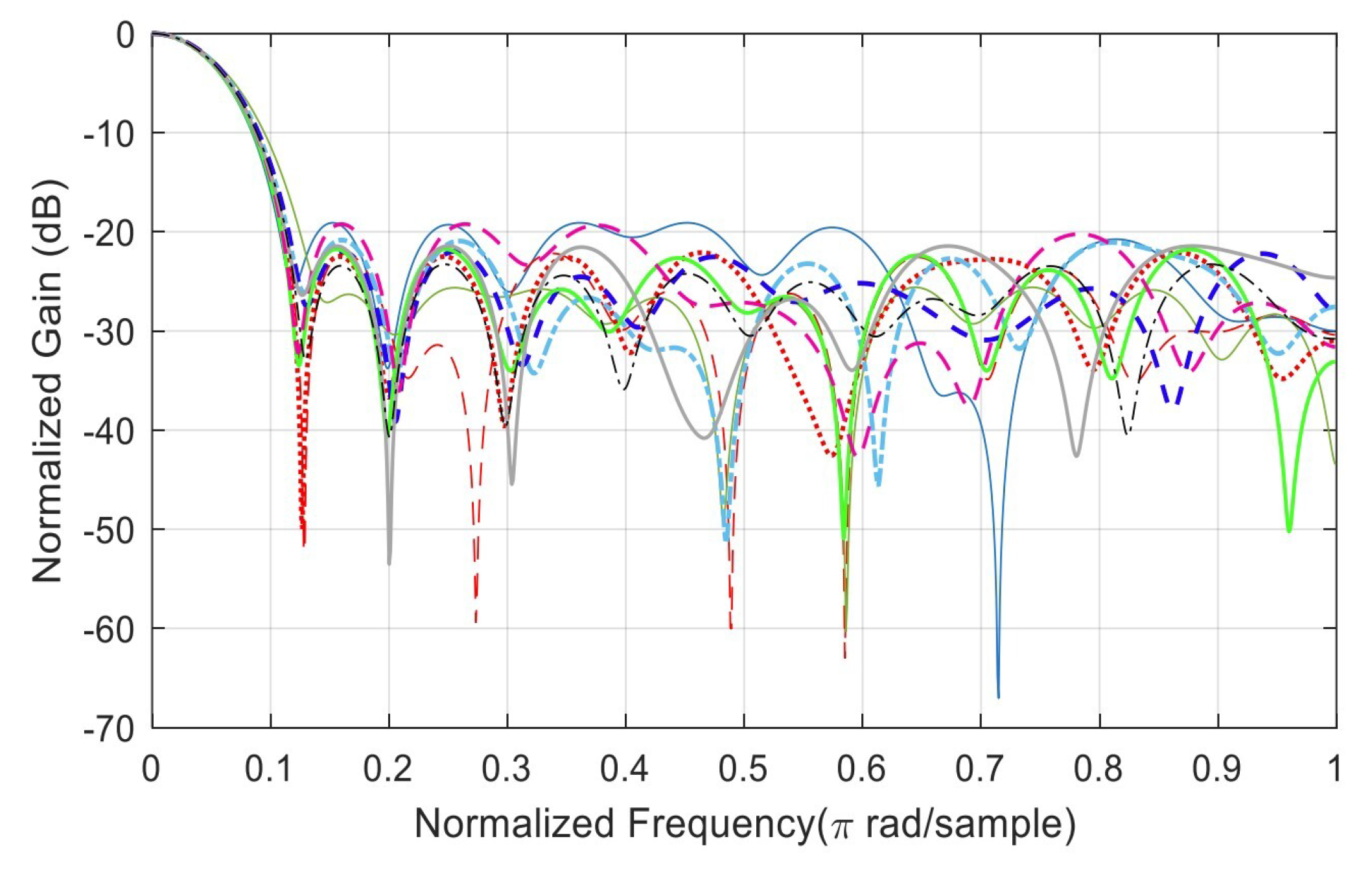
Figure A2 shows the minimization of the SLL. Ten (10) solutions for the Crossover/ Two-points. Worst case SLL: -28.8705 dB, Best case SLL: -31.7864 dB, Mean= -30.8800 dB, Median= -30.9479 dB. Ten SLL solutions = [-31.1692, -31.7864, -31.5800, -30.6253, -31.3180, -30.6638, -28.8705 -30.7265, -31.6496, -30.4102].
Figure A2.
Minimization of the . Ten (10) solutions for the Crossover/ Two-points.
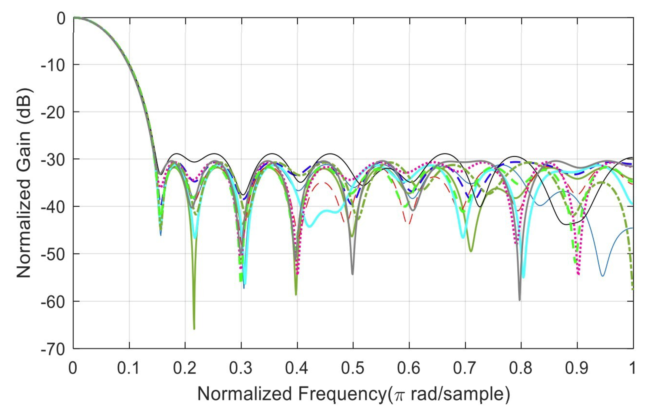
Figure A3 depicts the minimization of the SLL. Ten (10) solutions for the Mutation/ Adapt-Feasible. Worst case SLL: -30.7847 dB, Best case SLL: -31.7460 dB, Mean= -31.3768 dB, Median= -31.3983 dB, Ten SLL solutions = [-31.2148 -31.1336, -30.7847, -31.5693, -31.6100, -31.6331, -31.4939 -31.3027, -31.2802, -31.7460].
Figure A3.
Minimization of the SLL. Ten (10) solutions for the Mutation/ Adapt-Feasible.
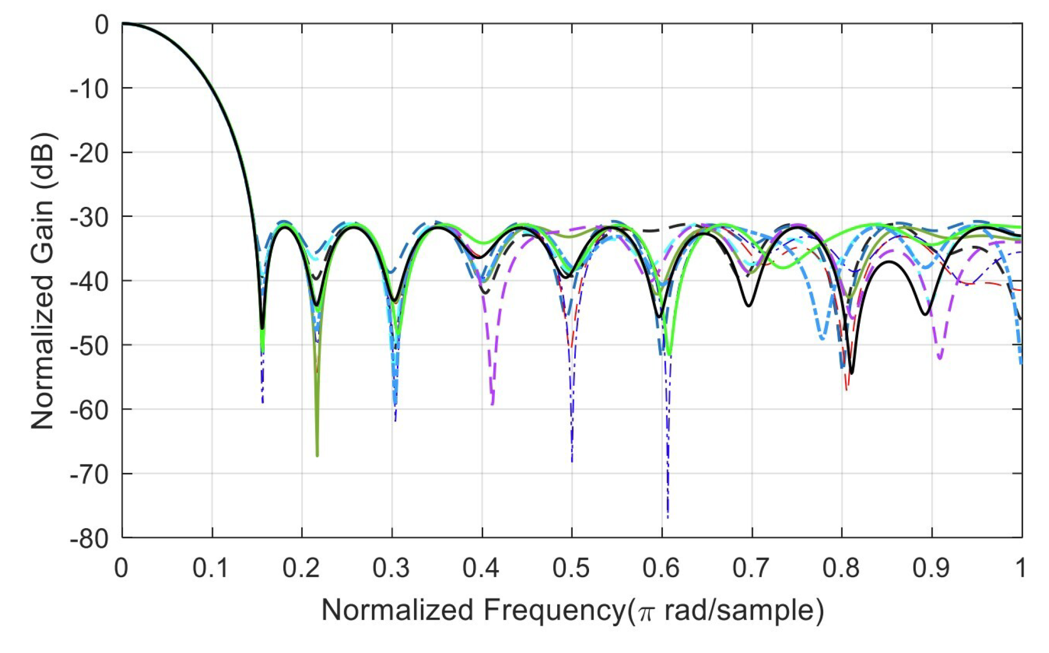
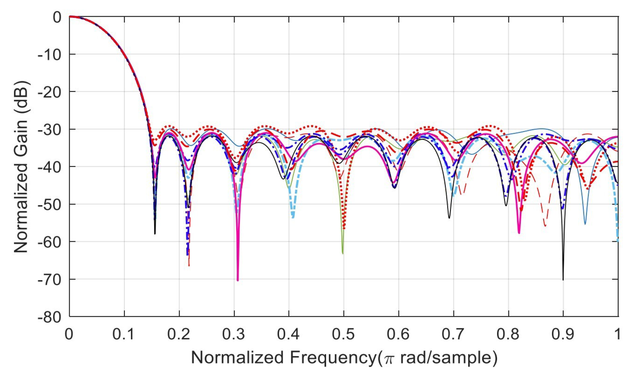
Figure A4 displays the minimization of the SLL. Ten (10) solutions for the Mutation/ Gaussian. Worst case SLL: -29.1817 dB, Best case SLL: -32.0514 dB, Mean= -30.9744 dB, Median=-31.2508 dB, Ten SLL solutions = [-29.8972, -31.7044, -31.2590, -31.4947, -29.1817, -31.2425, -31.0011, -32.0514, -31.8377, -30.0746]
Figure A4.
Minimization of the SLL. Ten (10) solutions for the Mutation/ Gaussian.
References
- Ansari, S.; Alnajjar, K.A.; Mahmoud, S.; Alabdan, R.; Alzaabi, H.; Alkaabi, M.; Hussain, A. Blind Source Separation Based on Genetic Algorithm-Optimized Multiuser Kurtosis. In Proceedings of the 2023 46th International Conference on Telecommunications and Signal Processing (TSP), 2023, pp. 164–171. [CrossRef]
- Figueroa-García, J.C.; Neruda, R.; Hernandez-Pérez, G. A genetic algorithm for multivariate missing data imputation. Information Sciences 2023, 619, 947–967.
- Digital Filters. In Time Series Data Analysis in Oceanography; Cambridge University Press, 2022; pp. 374–398. [CrossRef]
- Kaur, H.; Saini, S.; Raut, Y. The Application of Hybrid Optimization For FIR Filter Design. In Proceedings of the 2023 1st International Conference on Innovations in High Speed Communication and Signal Processing (IHCSP). IEEE, 2023, pp. 386–391.
- Gen, M.; Lin, L. Genetic algorithms and their applications. In Springer handbook of engineering statistics; Springer, 2023; pp. 635–674.
- Cosoli, G.; Spinsante, S.; Scardulla, F.; D’Acquisto, L.; Scalise, L. Wireless ECG and cardiac monitoring systems: State of the art, available commercial devices and useful electronic components. Measurement 2021, 177, 109243.
- Kolupaev, A.Y.; Tyapkin, V.N.; Dmitriev, D.D.; Ratushniak, V.N.; Tyapkin, I.V.; Smolev, I.A. Synthesis of a Filter of Phase-Domanipulated Signals with a Minimum Side-Lobe Level. Journal of Siberian Federal University. Engineering & Technologies 2023, 16, 497–508.
- Chauhan, S.; Singh, M.; Aggarwal, A.K. Designing of optimal digital IIR filter in the multi-objective framework using an evolutionary algorithm. Engineering Applications of Artificial Intelligence 2023, 119, 105803.
- Kockanat, S.; Karaboga, N. The design approaches of two-dimensional digital filters based on metaheuristic optimization algorithms: a review of the literature. Artificial Intelligence Review 2015, 44, 265–287.
- Alzahrani, A.; Kanan, A. Machine Learning Approaches for Developing Land Cover Mapping. Applied Bionics and Biomechanics, 2022.
- Eldos, T.; Kanan, A.; Aljumah, A. Adapting the Ant Colony Optimization Algorithm to the Printed Circuit Board Drilling Problem. World of Computer Science & Information Technology Journal 2013, 3.
- Eldos, T.; Kanan, A.; Nazih, W.; Khatatbih, A. Adapting the Chemical Reaction Optimization Algorithm to the Printed Circuit Board Drilling Problem. International Journal of Computer and Information Engineering 2015, 9, 247–252.
- Prakash, R.; Yadav, S.; Kumar Saha, S. A Metaheuristic Approach for the Design of Linear Phase FIR Differentiator. In Proceedings of the 2023 International Conference on Computational Intelligence and Sustainable Engineering Solutions (CISES), 2023, pp. 744–748. [CrossRef]
- Maghsoudi, Y.; Kamandar, M. Low delay digital IIR filter design using metaheuristic algorithms. In Proceedings of the 2017 2nd Conference on Swarm Intelligence and Evolutionary Computation (CSIEC). IEEE, 2017. [CrossRef]
- Bhowmick, C.; Dutta, P.K.; Mahadevappa, M. Computer Aided Classification of Benign and Malignant Breast Lesions using Maximum Response 8 Filter Bank and Genetic Algorithm. In Proceedings of the 2020 IEEE REGION 10 CONFERENCE (TENCON). IEEE, 2020. [CrossRef]
- Romsai, W.; Nawikavatan, A.; Hlangnamthip, S.; Puangdownreong, D. Design of Optimal Active Low-Pass Filter by Hybrid Intensified Current Search. In Proceedings of the 2022 Joint International Conference on Digital Arts, Media and Technology with ECTI Northern Section Conference on Electrical, Electronics, Computer and Telecommunications Engineering (ECTI DAMT & NCON). IEEE, 2022. [CrossRef]
- Stubberud, P. Digital IIR Filter Design Using a Differential Evolution Algorithm with Polar Coordinates. In Proceedings of the 2022 IEEE 12th Annual Computing and Communication Workshop and Conference (CCWC). IEEE, 2022. [CrossRef]
- Tripathi, K.K.; Kidwai, M.S.; Khan, I.U. Performance Analysis of Low Pass FIR Filter Design using Dynamic and Adjustable Particle Swarm Optimization Techniques. In Proceedings of the 2021 10th International Conference on System Modeling & Advancement in Research Trends (SMART). IEEE, 2021. [CrossRef]
- Miyata, T.; Asou, H.; Aikawa, N. Design Method for FIR Filter with Variable Multiple Elements of Stopband Using Genetic Algorithm. In Proceedings of the 2018 IEEE 23rd International Conference on Digital Signal Processing (DSP). IEEE, 2018. [CrossRef]
- Guliashki, V.; Marinova, G. An Approach for Coefficients optimization in Adaptive Filter Signal Equalization. In Proceedings of the 2022 29th International Conference on Systems, Signals and Image Processing (IWSSIP). IEEE, 2022. [CrossRef]
- Debnath, K.; Dhabal, S.; Venkateswaran, P. Design of High-Pass FIR Filter using Arithmetic Optimization Algorithm and its FPGA Implementation. In Proceedings of the 2022 IEEE Region 10 Symposium (TENSYMP). IEEE, 2022. [CrossRef]
- Chauhan, R.S.; Arya, S.K. An Optimal Design of FIR Digital Filter Using Genetic Algorithm. In Communications in Computer and Information Science; Springer Berlin Heidelberg, 2011; pp. 51–56. [CrossRef]
- Chandra, A.; Kumar, A.; Roy, S. Design of FIR filter ISOTA with the aid of genetic algorithm. Integration 2021, 79, 107–115. [CrossRef]
Figure 1.
Research Methodology Flow Chart.

Figure 2.
Structure of a direct form discrete-time FIR of order M.
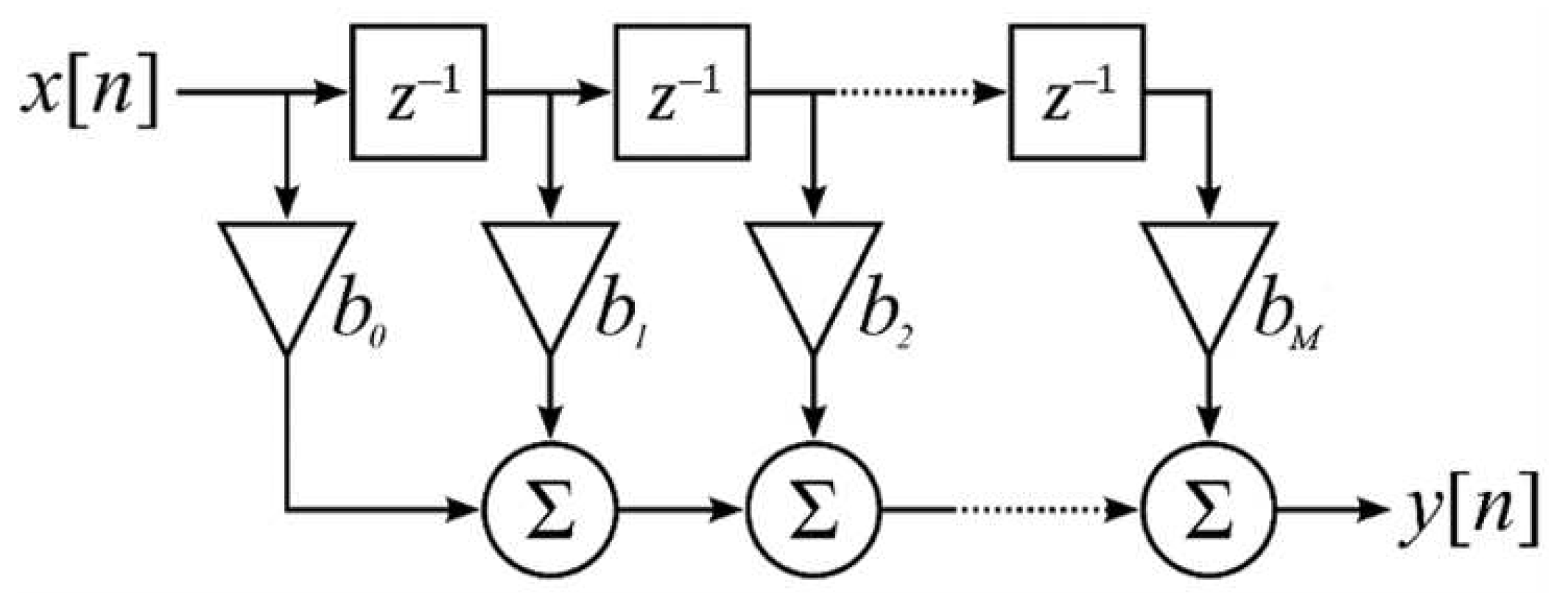
Figure 3.
General structure of a genetic algorithm for digital filter applications.
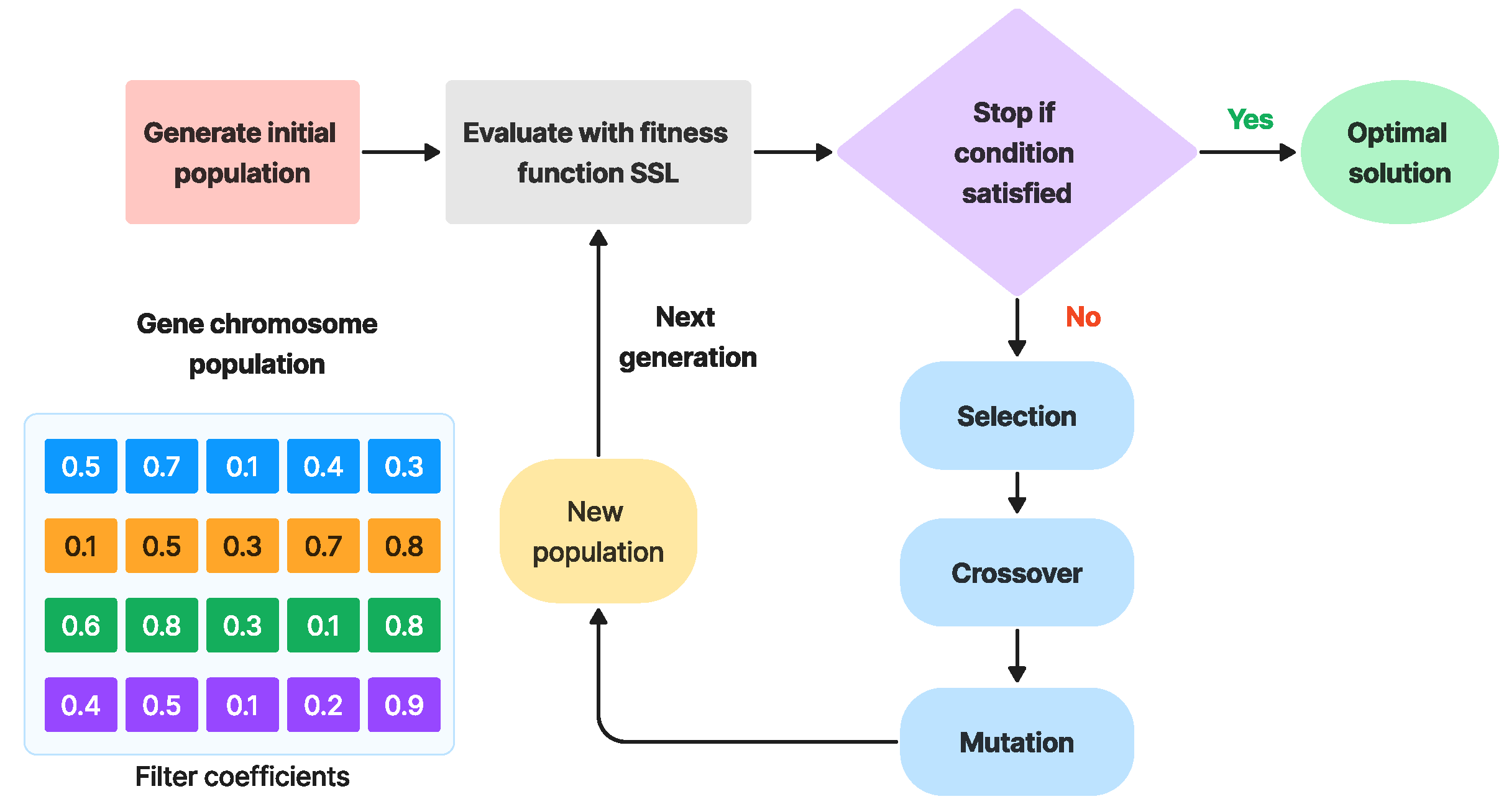
Figure 4.
A population of 20 filters (Chromosomes). The best filter is shown in red with minimum side lobe level (). Relative or normalized frequency is in logarithmic scale. The filter order is N-1=19.
Figure 4.
A population of 20 filters (Chromosomes). The best filter is shown in red with minimum side lobe level (). Relative or normalized frequency is in logarithmic scale. The filter order is N-1=19.
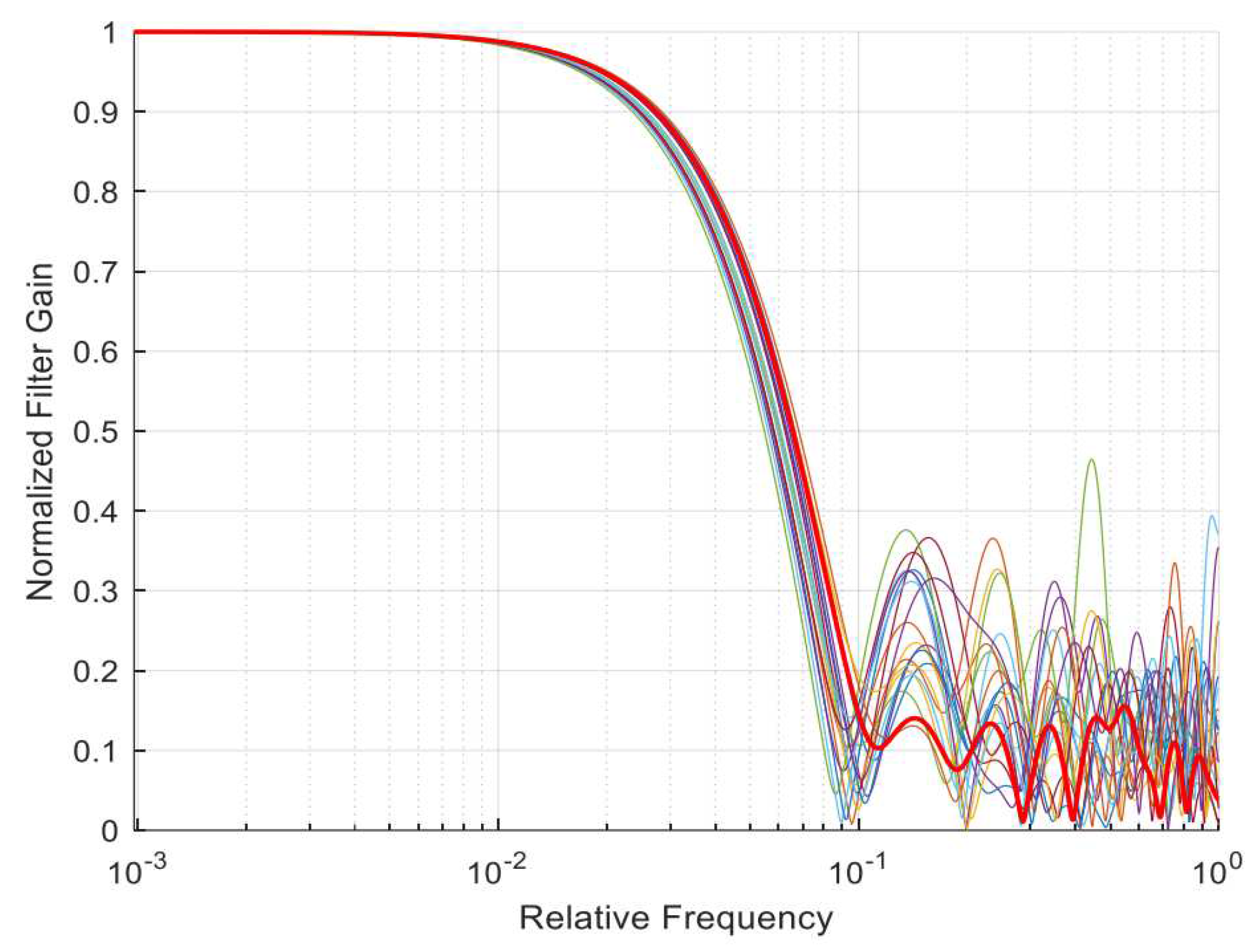
Figure 5.
The best filter based on the minimum selected from the initial population. The is at -16.166 dB. Relative or normalized frequency is in logarithmic scale. Filter order is (N-1) =19.
Figure 5.
The best filter based on the minimum selected from the initial population. The is at -16.166 dB. Relative or normalized frequency is in logarithmic scale. Filter order is (N-1) =19.
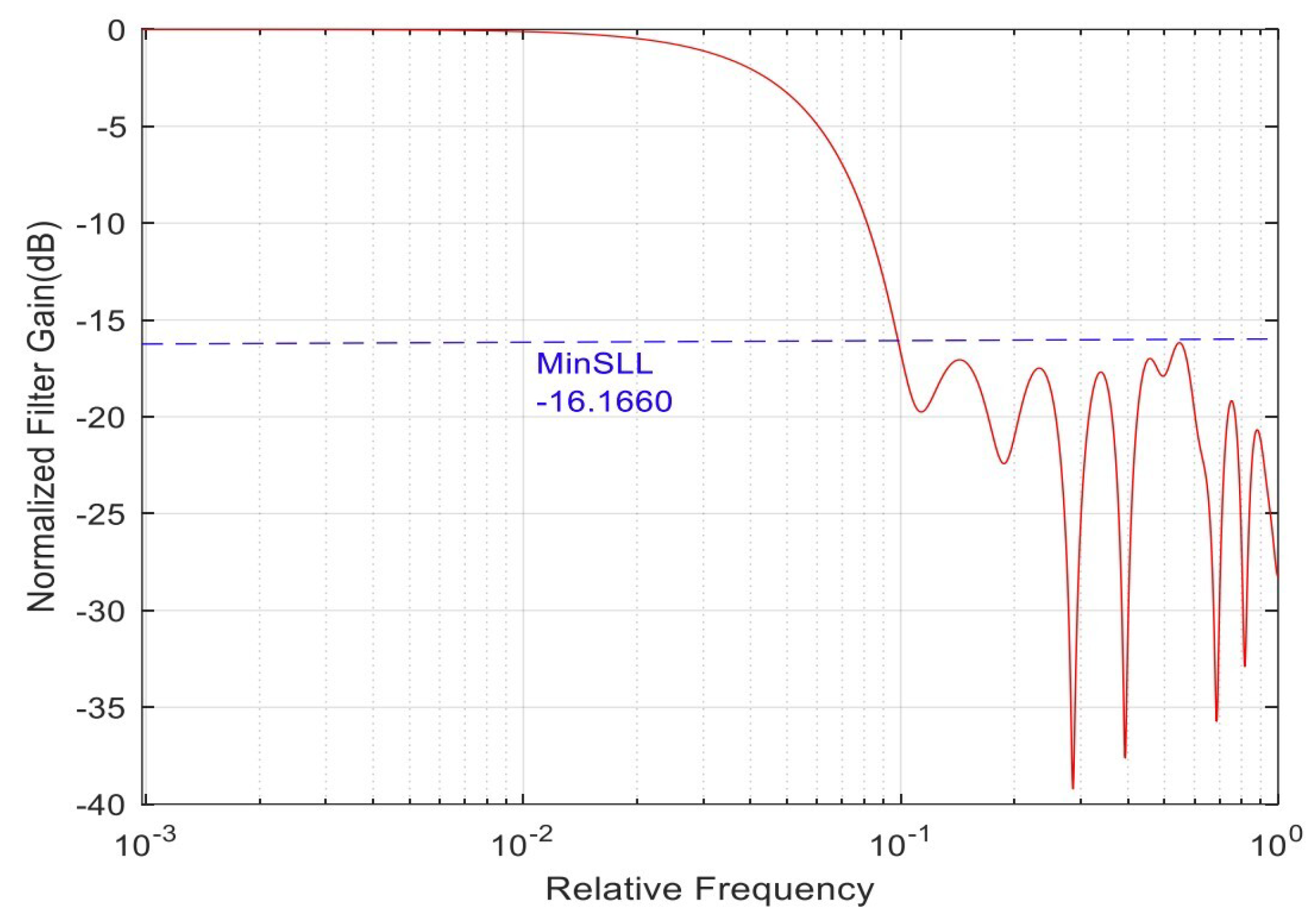
Figure 6.
Minimization of the . The magnitude spectrum shows two algorithm settings, each with two functions, as described in the legend.
Figure 6.
Minimization of the . The magnitude spectrum shows two algorithm settings, each with two functions, as described in the legend.
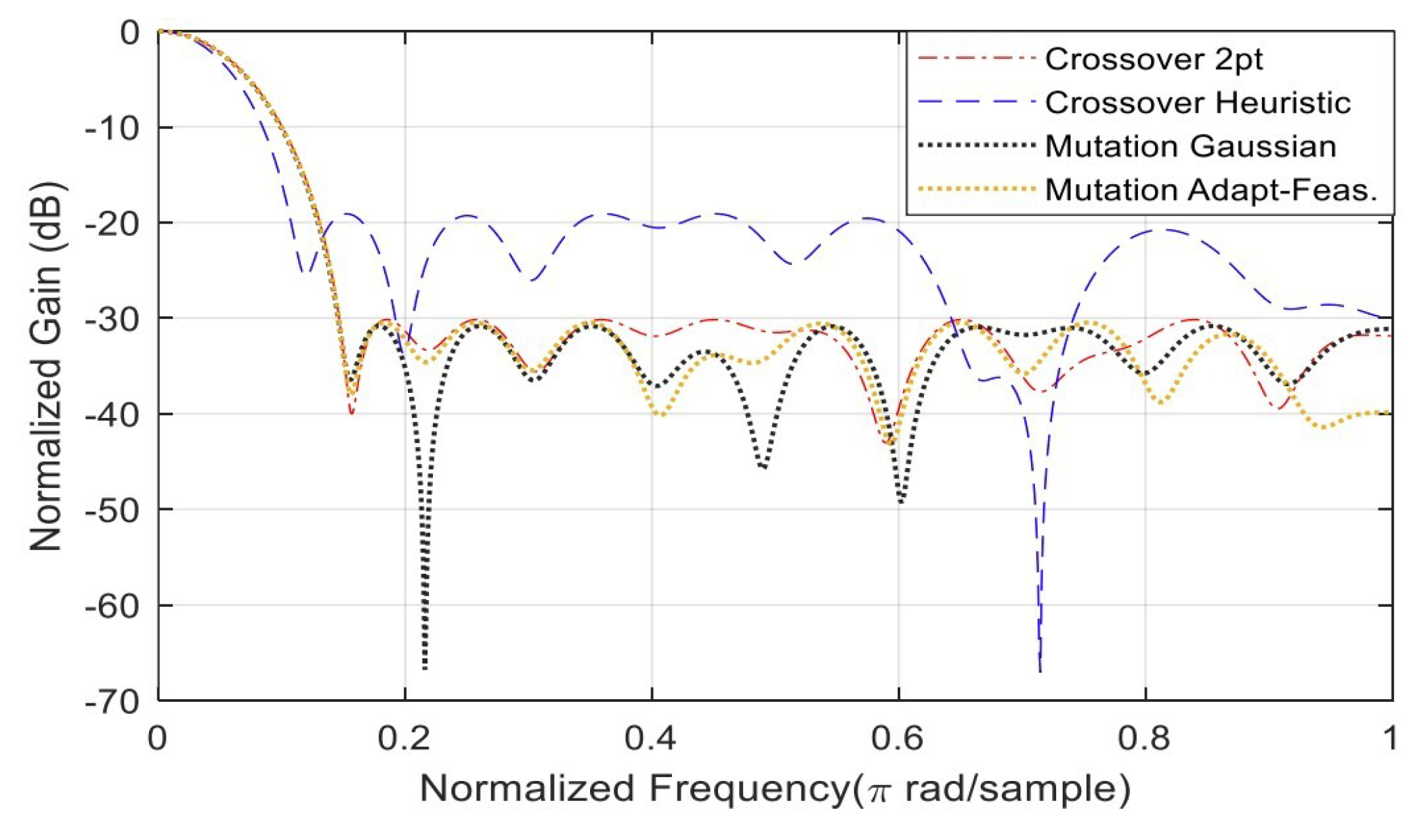
Figure 7.
Convergence speed of the minimization.
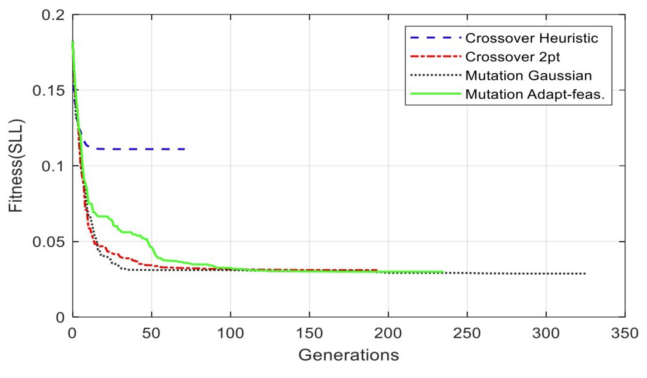
Figure 8.
Minimization of the SLL (max gen. 100 and 200).
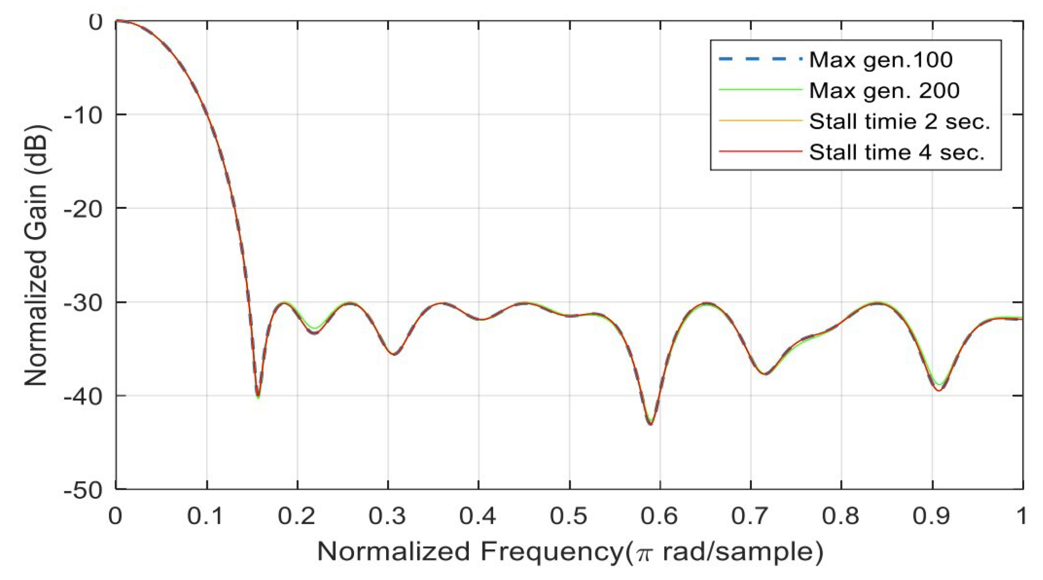
Figure 9.
Convergence speed of the minimization. For max generations of 100, the fitness stops exactly at 100 generations, while for the three other cases, the generations stop at 193 generations.
Figure 9.
Convergence speed of the minimization. For max generations of 100, the fitness stops exactly at 100 generations, while for the three other cases, the generations stop at 193 generations.
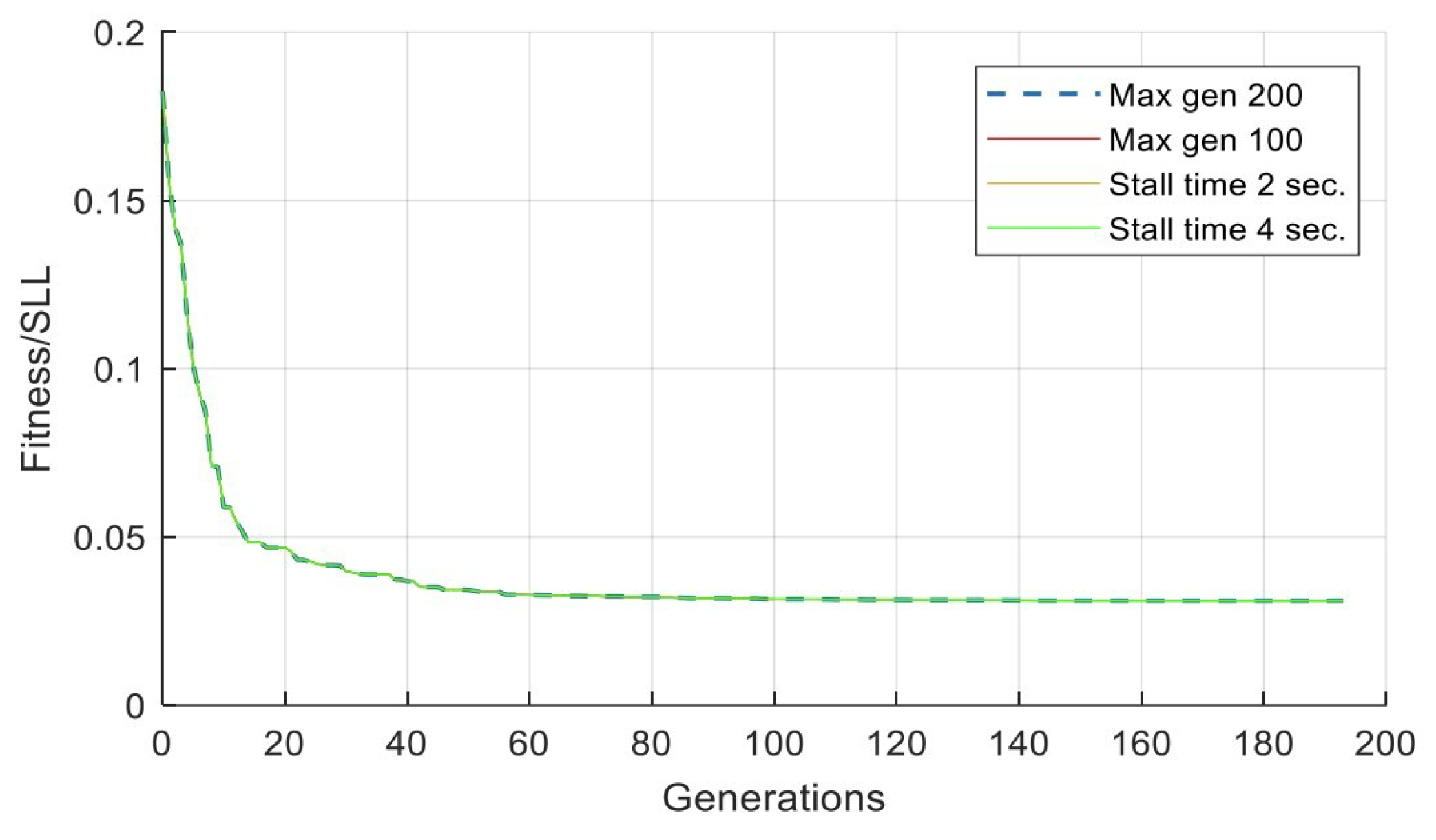
Figure 10.
Minimization of the . For population size increasing from 100 to 300, the decreases from -30.7976 to -31.5810 with a slight difference of less than 1 .
Figure 10.
Minimization of the . For population size increasing from 100 to 300, the decreases from -30.7976 to -31.5810 with a slight difference of less than 1 .
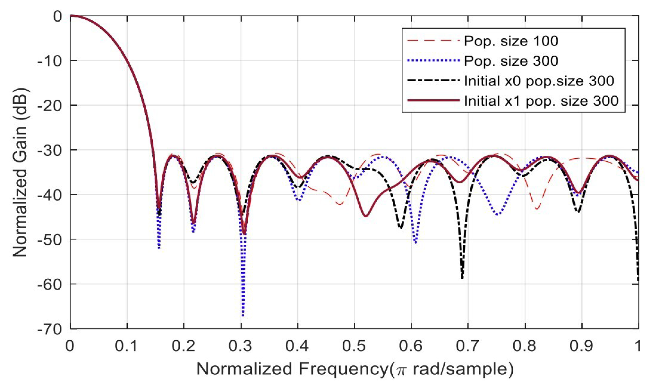
Figure 11.
Convergence speed of the minimization.
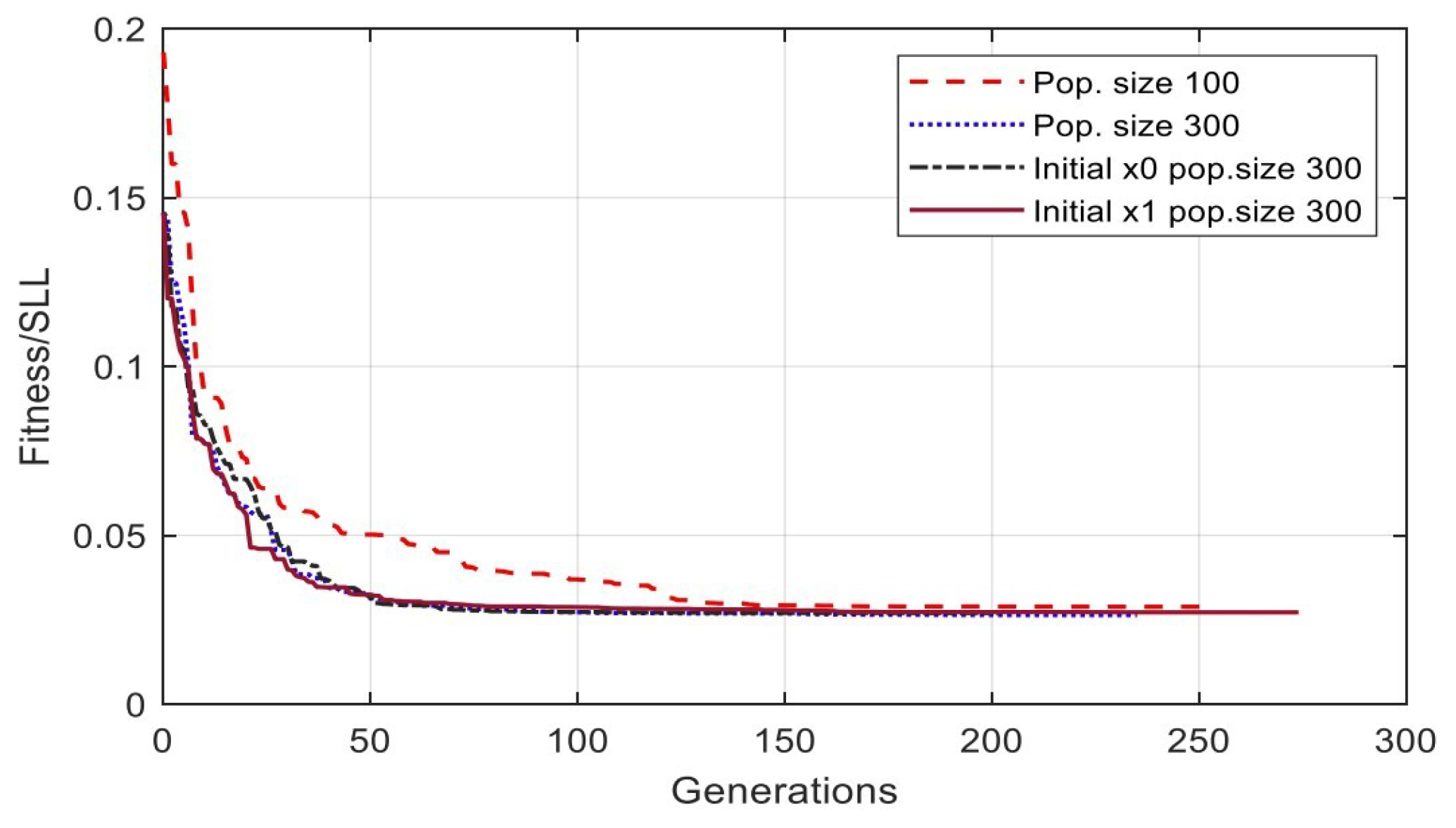
Figure 12.
Minimization of the changing the function tolerance from 1.e-5 to 1.e-4 shift the from -30.1490 dB to -29.9617 with faster convergence.
Figure 12.
Minimization of the changing the function tolerance from 1.e-5 to 1.e-4 shift the from -30.1490 dB to -29.9617 with faster convergence.
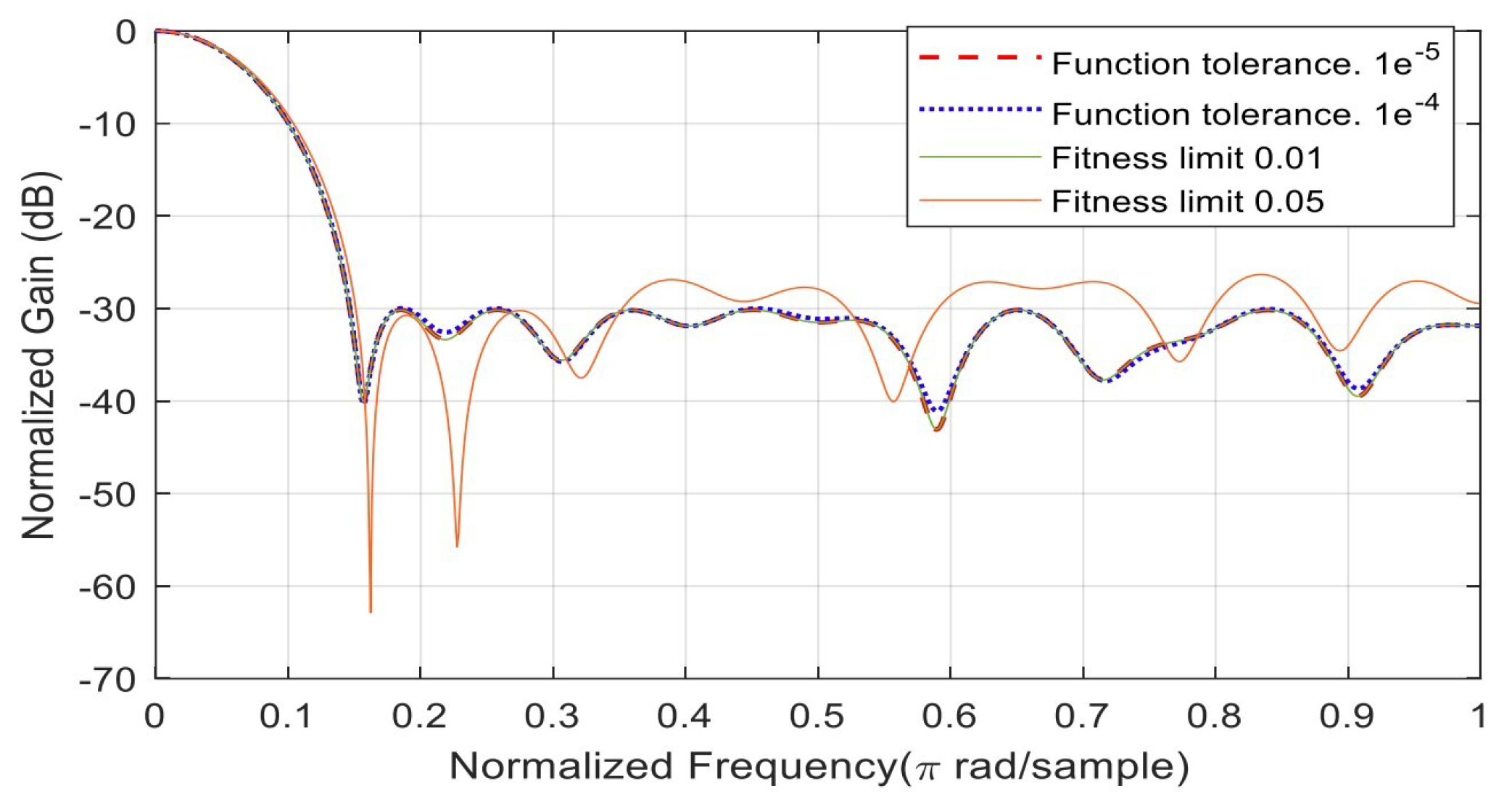
Figure 13.
Convergence speed of the minimization of different tolerance options.
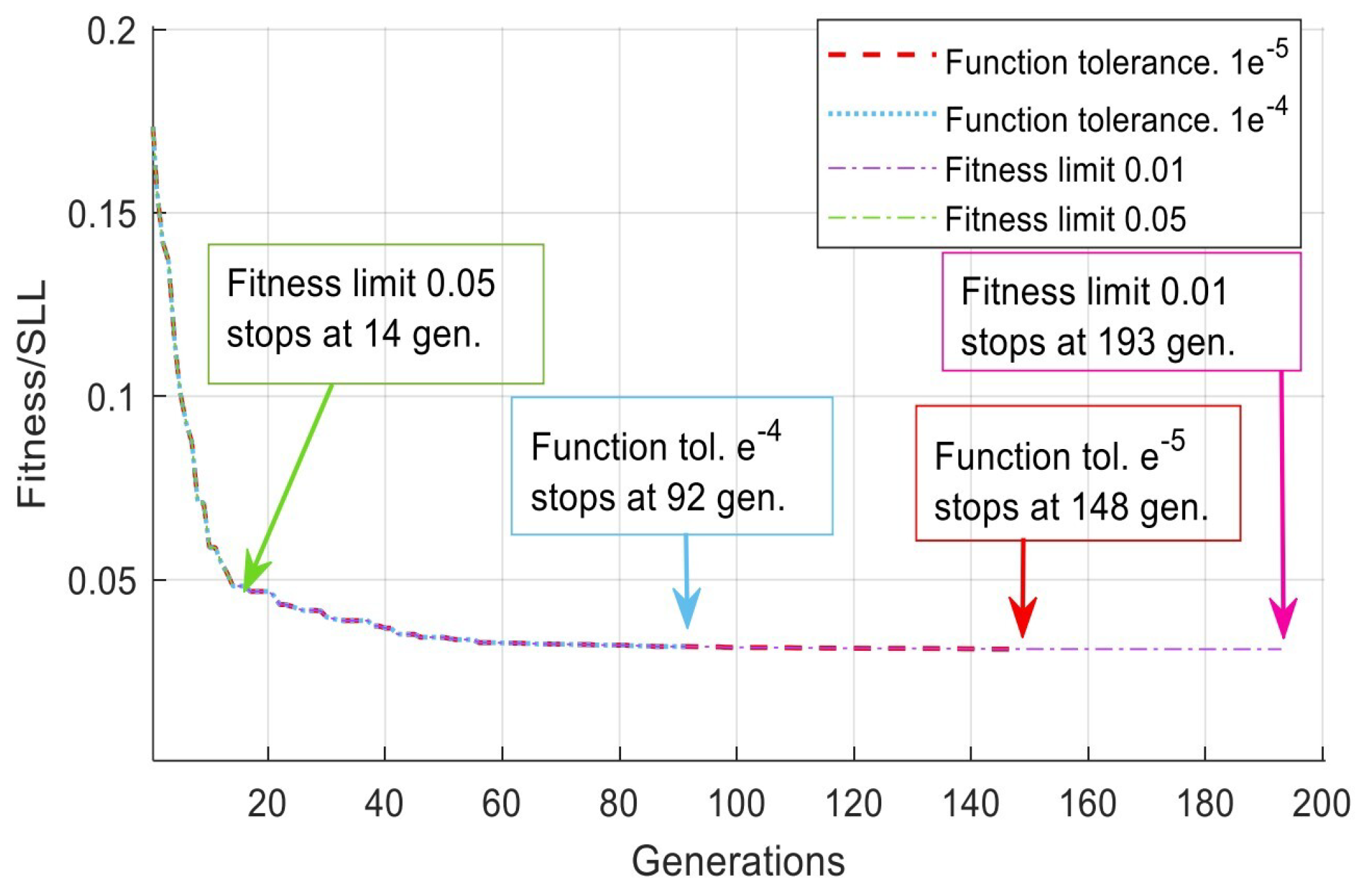
Figure 14.
Ideal ECG signal for a normal person.
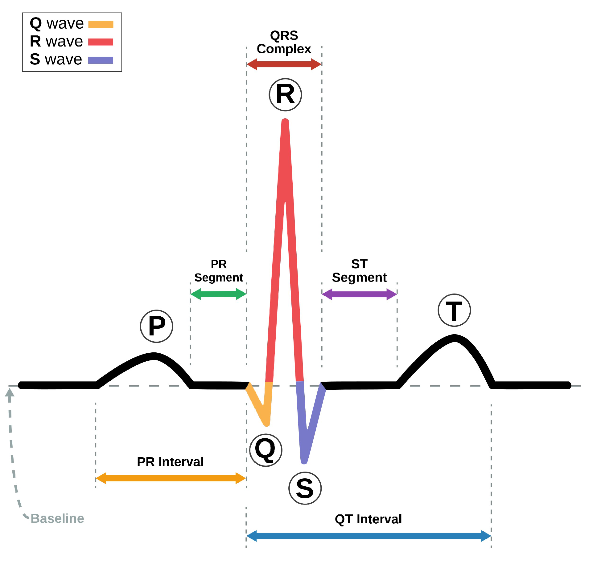
Figure 15.
Example of one second of the noisy ECG signal.
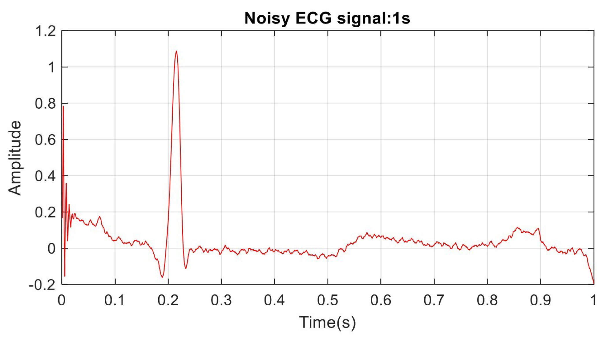
Figure 16.
The magnitude spectrum of the noisy ECG signal. The ECG signal is contaminated with a 60 Hz signal from the power line. The sampling rate is 720 samples/sec. Half sampling is at 360 Hz.
Figure 16.
The magnitude spectrum of the noisy ECG signal. The ECG signal is contaminated with a 60 Hz signal from the power line. The sampling rate is 720 samples/sec. Half sampling is at 360 Hz.
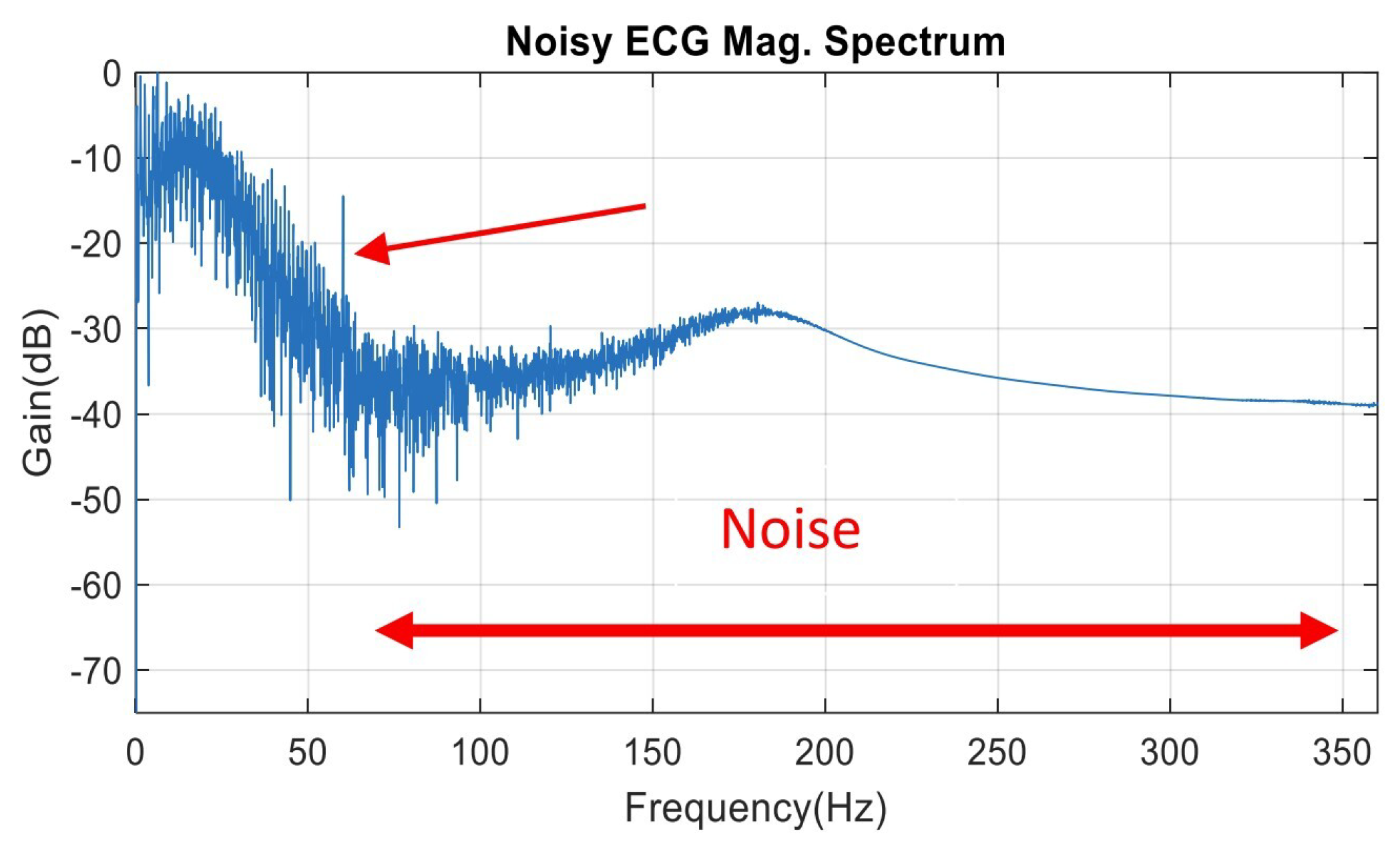
Figure 17.
Filtered ECG spectrum magnitude using GA Gaussian mutation.
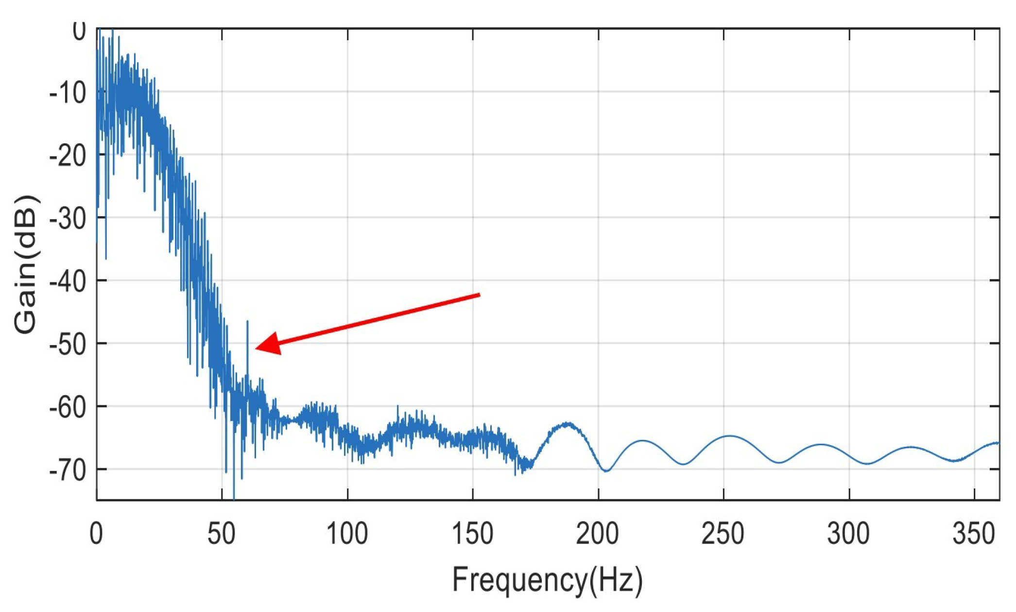
Figure 18.
One second at the beginning of the filtered signal showing complete removal of the artifact, 60 power signal interference with smoothed ECG signal using Gaussian mutation genetic algorithm.
Figure 18.
One second at the beginning of the filtered signal showing complete removal of the artifact, 60 power signal interference with smoothed ECG signal using Gaussian mutation genetic algorithm.
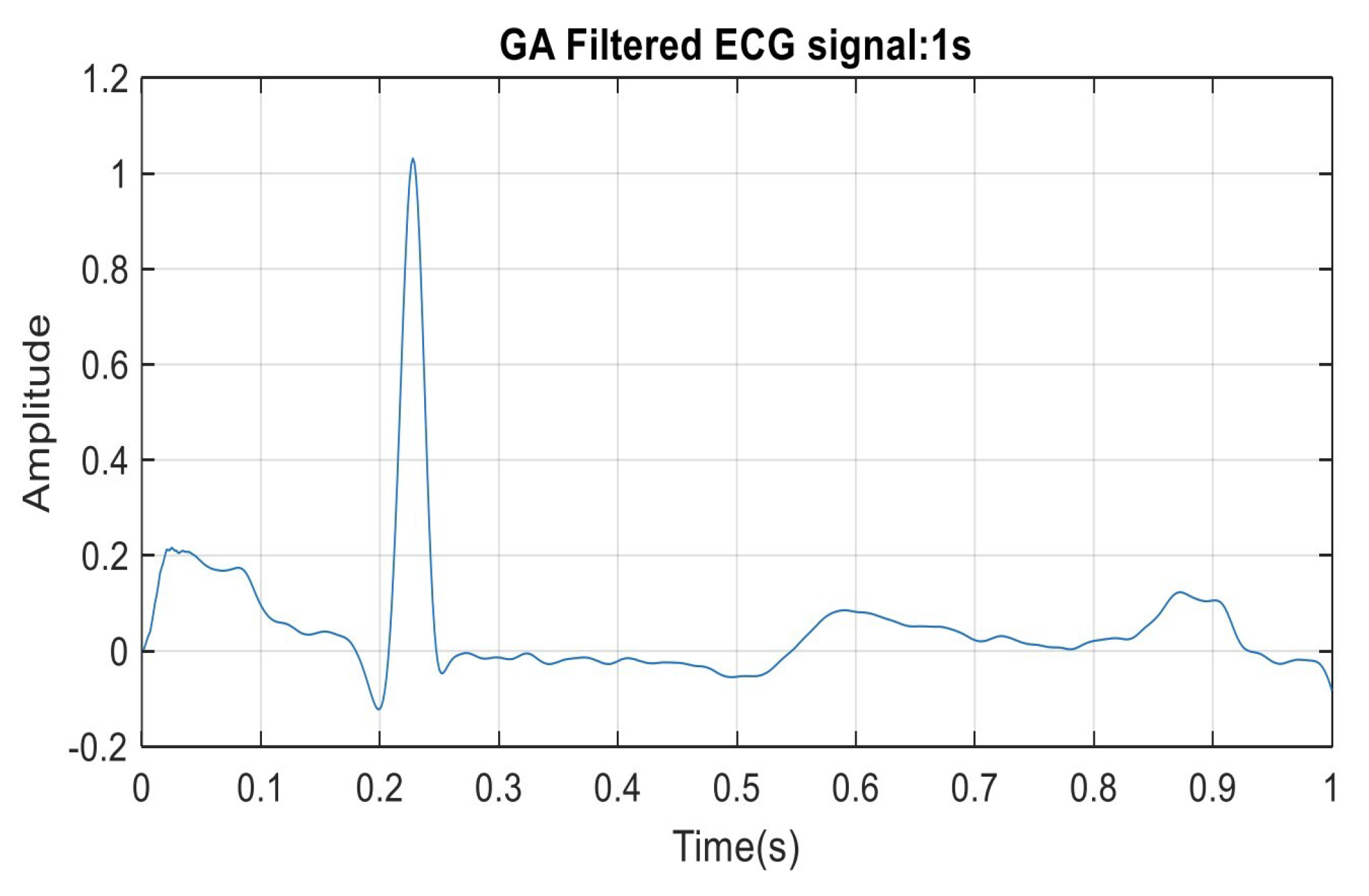
Figure 19.
Comparison between GA FIR filter and conventional FIR for low pass filters that generated by Matlab.
Figure 19.
Comparison between GA FIR filter and conventional FIR for low pass filters that generated by Matlab.
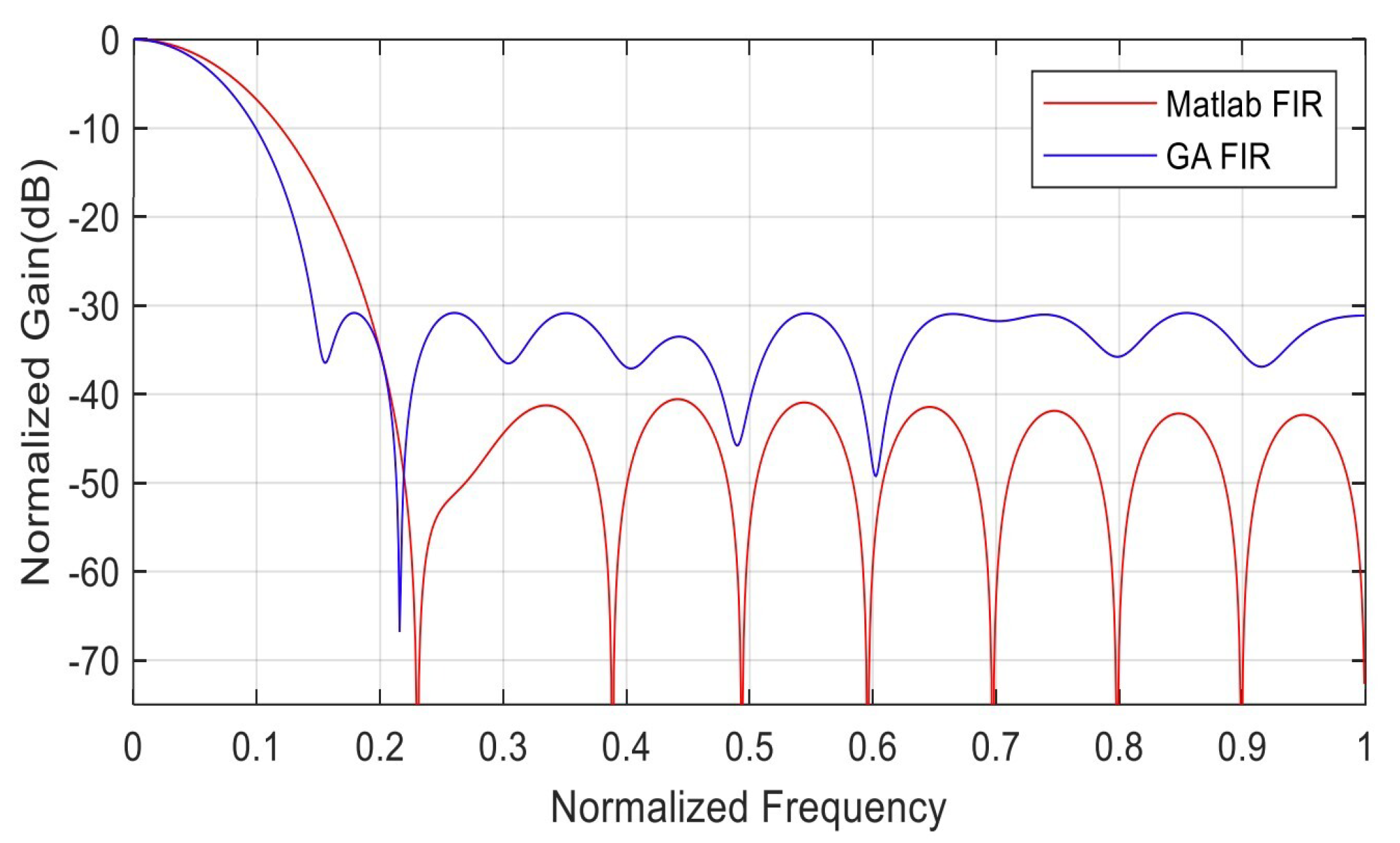
Table 1.
Algorithm setting evaluation results.
| Sub-function solver setting | Gen.No. Convergence | |||
|---|---|---|---|---|
| Cross Over | 1 | Heuristic | -19.0941 | 71 |
| Cross Over | 2 | Two points | -30.1599 | 193 |
| Mutation | 1 | Adapt Feas. | -30.4694 | 235 |
| Mutation | 2 | Gaussian | -30.8327 | 236 |
Table 2.
Population setting evaluation results.
| Sub-function solver setting | Gen.No. Convergence | |||
|---|---|---|---|---|
| Max gens | 1 | 100 | -30.0219 | 100 |
| Max gens | 2 | 200 | -30.1599 | 193 |
| Stall time limit | 1 | 2 Sec | -30.1599 | 193 |
| Stall time limit | 2 | 4 Sec | -30.1599 | 193 |
Table 3.
Run Time Limits.
| Sub-function solver setting | Gen.No. Convergence | |||
|---|---|---|---|---|
| Pop. Size | 1 | 100 | -30.7976 | 253 |
| Pop. Size | 2 | 300 | -31.5810 | 235 |
| Initial. Pop | 1 | Initial Pop. () | -31.3811 | 274 |
| Initial. Pop | 2 | Initial Pop. () | -31.3141 | 202 |
Table 4.
Tolerance evaluation results.
| Sub-function solver setting | Gen.No. Convergence | |||
|---|---|---|---|---|
| Fun. tolerance | 1 | -29.9617 | 92 | |
| Fun. tolerance | 2 | -30.1490 | 148 | |
| Fitness limit | 1 | 0.01 | -26.3296 | 14 |
| Fitness limit | 2 | 0.001 | -30.1599 | 193 |
Disclaimer/Publisher’s Note: The statements, opinions and data contained in all publications are solely those of the individual author(s) and contributor(s) and not of MDPI and/or the editor(s). MDPI and/or the editor(s) disclaim responsibility for any injury to people or property resulting from any ideas, methods, instructions or products referred to in the content. |
© 2020 by the authors. Licensee MDPI, Basel, Switzerland. This article is an open access article distributed under the terms and conditions of the Creative Commons Attribution (CC BY) license (https://creativecommons.org/licenses/by/4.0/).
Copyright: This open access article is published under a Creative Commons CC BY 4.0 license, which permit the free download, distribution, and reuse, provided that the author and preprint are cited in any reuse.


