
Submitted:
18 August 2023
Posted:
22 August 2023
You are already at the latest version
Abstract
An aneurysm is a vascular malformation, it can be classified according to its location (cerebral, aortic); and according its shape (saccular, fusiform, and mycotic). The study of blood flow interaction with the aneurysms has gained attention from physicists an engineers in recent years. Shear stresses, oscillatory shear index (OSI), gradient oscillatory number (GON), and residence time had been used as potential variables to describe the hemodynamics as well as the origin and evolution of aneurysm. However, the causes of aneurysms and the hemodynamics conditions that promote the growth of these structures are still under debate. The present work presents numerical simulation on three aneurysms: 2 aortic and 1 cerebral. The results shows that the blood rheology is not relevant for aortic aneurysms, however, for cerebral aneurysm could play a relevant role in the hemodynamics. The turbulence models evaluated show equivalent results in both cases. Lastly, a simulation considering the fluid-structure interaction (FSI) shows that this phenomenon is the dominant factor for aneurysms simulation.
Keywords:
Aneurysm
; CFD
; blood flow
; turbulence model
; rheology.
1. Introduction
An aneurysm is a vascular malformation, than can be classified according to its location (cerebral, aortic); and according its shape (saccular, fusiform, and mycotic). The study of blood flow interaction with aneurysms has gained attention from physicists and engineers in recent years [1]. Computational fluid dynamics (CFD) has allowed the use of pacient specific aneurysm geometries [2], substituting the numerical simulation and experimental measurements on idealized models [3].
Furthermore, CFD solutions allow the evaluation of hemodynamics parameters, like wall shear stresses (WSS) and oscillatory shear index (OSI); as potential variables to describe the origin an evolution of aneurysms [4]; and in recent years these parametes have been linked with the aneurysm rupture risk in combination with morphological parameters (size, shape and location) [5]. Therefore, it is of great importance to assure that the numerical results adequately describe the biological part. Selecting laminar or turbulent flow and the rheological model of the blood are factors that have a great impact on the numerical solutions.
The Reynolds number of blood flow in intracranial aneurysms is aroung 400 and a mean value of 600 for abdominal aneurysms [6]; therefore, according to the classical pipe theory the flow is laminar. Lee et al., [7] performed numerical simulations considering laminar flow to evaluate the size and shape of the aneurysm. Han et al., [8] also employed laminar flow in patient specif cerebral aneurysms for rapid evaluation and treatment planning. However, Poelma et al., [9] found that the flow in aneurysms is turbulent due the oscillatory nature of the blood flow. MoMoradicheghamahi et al., [10] found that turbulent models overestimated the time-averaged wall shear stress in stenosed carotid arteries, estimating less damage in the wall than the real value.
On the other hand, it is well known that blood is a non-Newtonian fluid and its rheological behaviour depends on the diameter of the vessel, the Fåhraeus–Lindqvist effect [11]. According to the characteristic length of abdominal aneurysm, the blood can be considered as a Newtonian fluid. For intracranial aneurysms, the mean arteries diameter is around 1 [mm], and the rheology is in the limit between Newtonian and non-Newtonian. Abbasian et al., [12], studied the influence of rheological models in atherosclerotic coronary arteries, considering the most common models used in numerical simulations are Casson, Carreau, and power law. They found that Carreau, modified Casson, and Quemada viscosity blood models were the most accurate; however, the results shown that blood flow can be considered laminar in some sections with high WSS. Abugattas et al., [13] analyzed the influence of the power-law, Cross, and Carreau–Yasuda models in the carotid artery flow pattern, their results shown that the power-law estimates lower WSS in comparison to the other models.
A third effect that is relevant in the blood flow simulation in aneurysms is the elastic properties of the wall. Most of the numerical simulations employed the rigid wall considerations ([14,15]); however, the cerebral arteries are deformable, therefore the FSI must be considered ([16,17]) . According to Moradicheghamahi et al., [10] the elastic wall has a major effect on the CFD analysis than the rheology or laminar/turbulent flow.
The use of turbulent and rheological models to numerically describe the flow in intracranial aneurysms is still under debate, as well as the rigid or elastic artery wall. In the present work a comparison of a turbulent model ( model) and laminar model is done for three aneurysms, two aortic aneurysms (AAA1 and AAA2) and a cerebral aneurysm (IA). Four rheological models are evaluated: newtonian, power-law, Carreau and Casson. Finally, the rigid wall solutions are compared with the aneurysms with elastic wall. Wall shear stress (WSS), time average wall shear stress (TAWSS), oscillatory shear index (OSI), relative residence time (RRT), and gradient oscillatory number (GON) were calculated for each case, according to the definitions given by [18], and the results were compared with the laminar case.
2. Materials and Methods
To assess the influence of blood rheology, turbulence models, and wall elasticity on the fluid dynamics in aortic and intracranial aneurysms numerical simulations were performed. Patient-specific cases were employed to rebuilt the geometries.
2.1. Governing equations
With the geometry defined, a CFD simulation implemented in OpenFOAM [19] software was used to solve the mass and momentum conservation equation,Eq. 1 and Eq. 2 respectively, under the assumptions of blood as a homogeneous incompressible fluid and taking into account that the fluid flow is isothermal. Therefore, the Navier-Stokes equations can be written as:
Where is the velocity vector, is density, t is time, and p is pressure field. To evaluate the influence of blood rheology, the Newtonian, Carreau, Casson, and Power-law rheological models were used to describe the behaviour of blood viscosity () in two abdominal aortic aneurysms (AAA) and an intracranial aneurysm (IA).
Newtonian fluid is characterized by a linear relationship between shear stress and shear rate. The relation is , where is the stress tensor, is the fluid viscosity, and is the rate-of-strain tensor. On the other hand, the simplest non-Newtonian model is the power-law, where the relation between the shear stress and shear rate is non-linear, defined as:
Where n is the power-law index, and K is the consistency index. For , Eq. 3 describes a dilatant fluid; meanwhile, for a pseudoplastic or shear-thinning fluid is obtained. In shear-thinning fluids, like blood, the shear rate increases while the apparent viscosity decreases. The drawback of this model is that it can overestimate or underestimate the viscosity at very high or very low values of strain rates, respectively, which may not have a physical sense.
In order to describe properly the shear-thinning blood behaviour, two models had been defined. The first one is the Cassson model, given by:
Where is interpreted as the yield stress and m is a viscosity consistency. The second one is the Carreau model, which provides a smooth transition between the viscosity limit values, given by the equation:
and are the minimum and maximum viscosity limit values obtained experimentally. is the viscosity value when the blood is not subjected to shear stress, and is the minimum viscosity value reached after a large strain-rate (>100) is applied. Commonly, the value is used as the Newtonian constant value. The non-Newtonian behavior is described by the time and the exponent n, where . The parameters used in the rheological models are shown in the Table 1.
2.2. Transport equations for the standard model.
The model was used to study the influence of turbulence on the hemodynamic in aneurysms. The model solves the equations of kinetic energy (6) and the dissipation of kinetic energy (7) to determine the turbulent viscosity (8).
Where k is the kinetic energy, is the dissipation of k, is the generation of kinetic turbulence by the mean velocity gradients; , , and are constants. The constant values have the following default values: , , , , according to [10].
2.3. Fluid-Solid Interaction (FSI)
In order to study the effect of the rigid artery wall simplification on the results, a FSI simulation was developed in AAA2 where the linear elastic model was chosen to model the elastic behavior of the artery wall. Bazilevs et al. [24] and Torii et al. [25] concluded that the linear elastic model is a good approximation to model the wall elasticity, after compare differents wall models.
Mechanical properties of the wall tissue are considered uniform, and were based on Isaksen et al. [26]: , , , and wall thickness of 2 mm.
The solid momentum equation with the linear elastic consideration is written as follows:
Where is density, is displacement tensor, and are the Lame constants, and I is the second order tensor.
2.4. Boundary conditions
For the reological and turbulence analysis, the artery wall was assumed to be rigid, and the no-slip boundary condition was applied. A pulsatile flow was defined at the inlet, using the waveform from Banerje et al. [27], with a mean Reynolds value of 600 in AAA, and 400 in IA. In the outlet branches, a pressure value of 0 was imposed. Density was consider constant with 1056 value. Viscosity () depends on the rheological model. Six cardiac cycles were used to do the transient simulations, as the condition for the existance of the periodic solution, and the results of the last cycle were analyzed.
For FSI case, the inlet and outlet boundary conditions of the rigid wall case were employed. The displacement of the fluid and solid interfaces must be the same (Eq. 10), and the traction in both domains must be in equilibrium (Eq. 11). Furthermore, the fluid obeys the non-slip condition on the solid wall. The solid sides are fixed, zero displacement, and a pressure of 0 Pa was imposed on the external wall.
The time step was variable to maintain a Courant number less than 0.1, for numerical stability. A second-order scheme was used to discretize the governing equations.
2.5. 3D Model
The patient-specific aneurysms geometries were extracted from digital subtraction angiography (DSA) images, using the open-source software 3D Slicer. To isolate the area of the aneurysm and the parent vessel, the threshold tool was used to distinguish blood from the rest of the tissues. The artery and the tissue around the artery were removed, the 3D model was exported to STL format, which was used to mesh the analyzed geometry in the simulation. The aortic aneurysms (AAA1 and AAA2) and cerebral aneurysm are shown in Figure 1
2.6. Grid generation
Mesh generation of the computational models was performed using the OpenFOAM’s tool snappyHexMesh. The mesh was hexahedral dominant, and a prismatic boundary layer was implemented to capture accurately the influence of the wall and the WSS.
Three cases were studied: two abdominal aortic aneurisms, (AAA1) and (AAA2), and an intracranial aneurysm (IA), Figure 1. A mesh independence test was developed in each model. In the abdominal aortic aneurysm (AAA1), three different meshes were created, with 460k (coarse), 620k (medium), and 935k (fine) elements. In order to compare the results of these three meshes, the area-average WSS of the last cardiac cycle was analyzed and plotted (Figure 2). The maximum difference of the fine and coarse mesh was 5 %, and respect with medium mesh, the maximum difference was 3 %. In the second abdominal aortic aneurysm (AAA2), the meshes studied comprised 525k (coarse), 670k (medium), and 1200k (fine) elements. The maximum difference of area-average WSS between fine and coarse meshes was 8 %, and in comparison with medium mesh the maximum difference was 3%. In the last model, the intracranial aneurysm (IA), the meshes studied comprised 200k (coarse), 300k (medium), and 2000k (fine) elements. The maximum differences comparing the fine mesh with the coarse and medium mesh were 7% and 4%, respectively. The meshes selected to do the rheological and turbulence analysis were the medium meshes in all the models, that have a percentage error less than 5%.
A wall turbulence model was employed, for the three cases was the maximum value obtained, meanwhile the maximum average value was . Therefore, the turbulent boundary layer can be resolved correctly. Besides, the mesh for the solid artery wall in the FSI study was achieved by extruding the fluid wall, with a constant thickness of 2 mm, built by 5 layers with an expansion ratio of 1.2. This method allows the match between the fluid and solid meshes.
3. Results
Velocity, wall shear stress (WSS), time average wall shear stress (TAWSS), oscillatory shear index (OSI), relative residence time (RRT), and gradient oscillatory number (GON) were calculated, according to the definitions given by [18]. The WSS was determined for systole and diastole; meanwhile, the other parameters where calculated for the last cardiac cycle. In this section the most relevant Figures are shown, the repository [28] shows the figures of all cases.
The indices for IA, Figure 3, shows higher values of WSS for systole, being the dominant effect on the TAWSS. The circled areas in the figure indicate the zones of low WSS and high values of OSI, RRT and GON. The results of IA, which have an aspect ratio (AR) of 1.13, shows that the blood flow goes upstream through the parent artery (ICA), impacting the distal side of the neck, then the flow goes towards the aneurysm dome, and finally returns to the parent vessel by the proximal side of the neck, completing one vortex, as was described by Munarriz et al. [29]. The highest value of WSS was found in the distal neck because of the impinging flow, while the values of WSS in the dome depend on the velocity distribution in the sac. Meng et al. [30] proposed that the growth and rupture of an aneurysm is associated with high or low values of WSS, depending on aneurysm shape and flow behavior. The numerical results shows that the IA belongs to the slow recirculation class, according to [30]. High values of OSI and low values of WSS can trigger inflammatory-cell-mediated destructive remodeling that leads to large, thick wall aneurysm phenotype.
In the aortic aneurysms (AAA1 and AAA2), Figure 4, the flow descends through the aorta to the aneurysm zone, where multiple vortices develop; furthermore, the results exhibit some areas with recirculation and stagnation flow. The circled areas meet the condition of low WSS and high OSI and RRT. Almost all the proposed indices points areas with high probability of destructive wall remodeling, according to [30]; except GON, that presented zones of high values in different parts of the aneurysm and its influence it is not clear.
3.1. Rheology
The strain rate results, Table 2, were calculated at the artery wall, at the aneurysm wall, at the blood volume in the artery (artery body), and finally at the blood volume in the aneurysm (aneurysm body). The strain rate values at the wall for IA were significantly higher that the AAA cases. As was expected, the strain rates in the fluid were lower than the values at the wall; however, IA cases presented values an order of magnitude bigger than the AAA. The values are relevant in order to determine the rheology influence on the flow behaviour.
The IA strain rate values were higher than the AAAs. The IA strain rate values in the total artery wall and the aneurysm wall were the order of . While the strain rate values in the total artery body and only the aneurysm body were highest than . AAAs values in the wall are near to 100, which is the critical strain rate value where the viscosity starts to behave like a constant Newtonian value in the no-Newtonian models. Values in the body far away from the wall are low, and differences between Newtonian and non-Newtonian models are expected.
The results of the rheological analysis in intracranial aneurysms show minimal differences between the models, considering the different indices under study with similar qualitative results between the Newtonian and non-Newtonian models. This can be explained because the strain rate is larger than 100 in the body and the aneurysm wall, as shown in the Table 2. AAAs results shown greater differences than IA in the studied indices. AAA2 was the most critical case, showing greater differences that could be attributed to low values of strain rate, even in the wall.
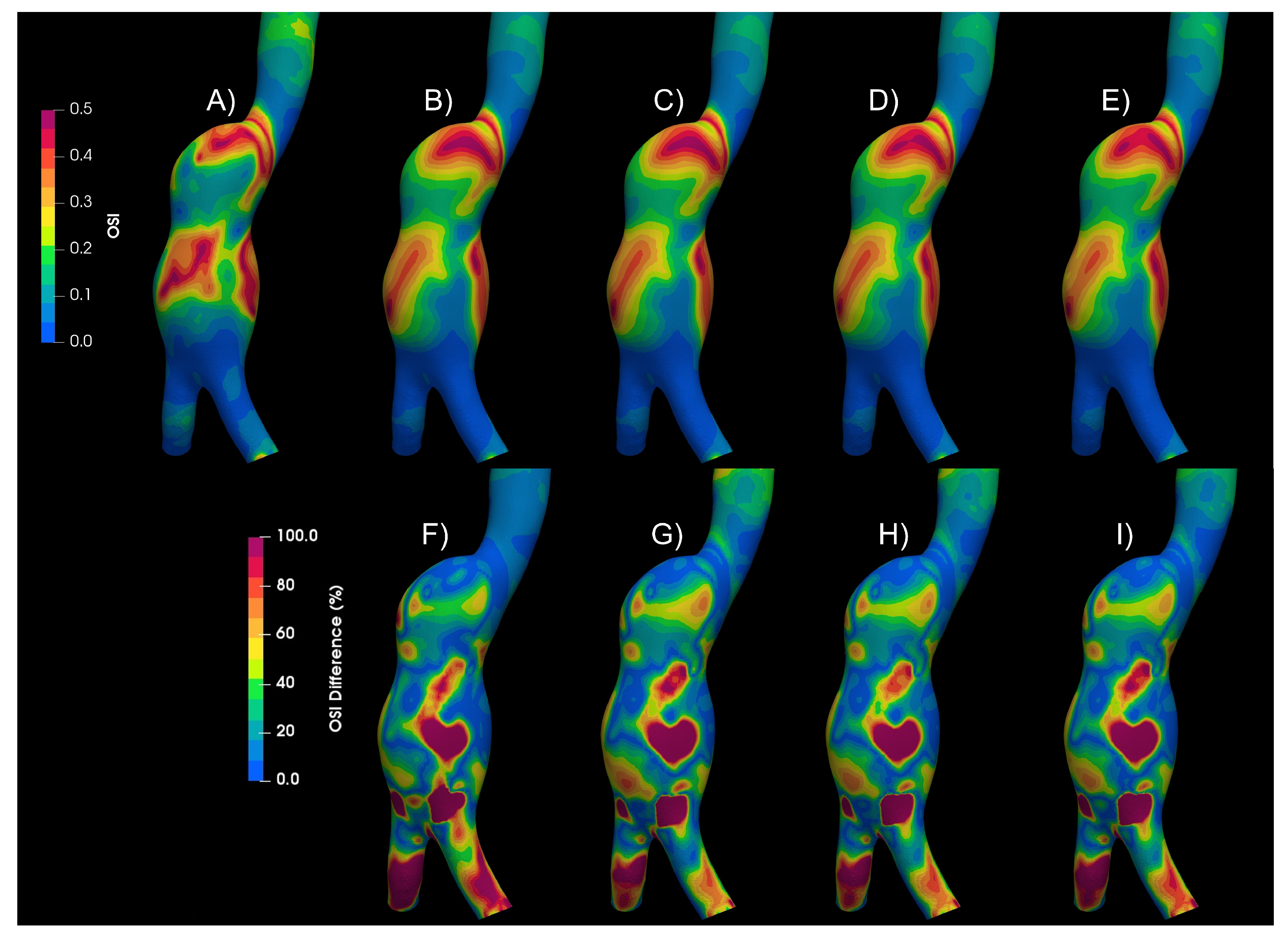
Figure 5 shows the Oscillatory Share Index (OSI) contours for the Newtonian and the non-Newtonian models, qualitative differences in the patterns can be observed. Below the OSI contours, (A to D), the differences of each of the non-Newtonian vs Newtonian models are shown, (E to G), some areas with differences of up to 100% can be seen. Similar differences were found in WSS, TAWSS, RRT and GON, repository.
In aortic aneurysms, far away from the wall the strain rate values are low, and the viscosity values differ from the Newtonian case. Therefore, the velocity profiles differ between newtonian and non-Newtonian models, as can be seen in the Figure 6, where the magnitude of velocity of the Newtonian and Carreau models are compared. The Newtonian model presents higher velocity values, and 25% of the plane area had a 50% difference or higher.
3.2. Turbulence
Turbulence is a complicated phenomenon, that is characterized by a caotic and instable flow. It is well known that for flow in pipes the critical Reynolds number () is . For lower a laminar flow can be considered, and for upper turbulent behaviour starts. In the present study a pulsatile flow was taken into account [27], and according to the physiological conditions a mean Reynolds number was used for AAA, with variations of to , with a Womersley number . For IA the following data were taken into account: , , , and a .
According to the classical theory in pipes, the blood flow in the aneurysms is laminar. However, Poelma et al., found differences in the velocity fields between the cycles under analysis Poelma et al. [9]; this changes are a characteristic of turbulent flows. The geometry of the aneurysms and the pulsatile nature of the flow are perturbations of the laminar flow and could modified the cirtical Reynolds number. Furthermore, the deceleration in the cardiac cycle is a destabilizing factor of the laminar flow; therefore Hershey and Im [31], NEREM and SEED [32], concluded that the critical Reynolds number is inversely proportional to the Womersley number.
To determine if the flow is laminar or turbulent, the results of 4 cardiac cycles were compared for both types of aneurysms. Differences between each cardiac cycle were found for aortic aneurysms, Figure 7; which is a characteristic of turbulent flows Poelma et al. [9]. On the other hand, for intracanial aneurysms no significant changes were observerd between cardiac cycles; therefore, the flow in IA can be considered as laminar.
Numerical simulations for both types of aneurysms were performed considering lamninar flow and Newtonian model, turbulent flow (using the K-epsilon model) and four rheological fluids : Newtonian, Carreau, Casson, and power-law. Figure 8 shows the WSS, TAWSS, OSI, GON, and RRT for an aortic aneurysm (AAA2) of the mentioned cases and the differences between them. The areas where the greatest differences occur between a laminar and a turbulent flow are marked in the figure (red circle). Differences exceeding 100% of the laminar value were found in large areas of the aneurysm, which overestimate the WSS, and consequently the TAWSS (lower part of the aneurysm); and promoting changes in the patterns of OSI, GON, and RTT in the central part of the aneurysm. Small differences (less than 5%) were obtained between the rheological models using the K-epsilon model, suggesting that the turbulent models are more relevant than the rheological characterization of the flow. This same behaviour was obtain for the second aortic aneurysm (AAA1). Meanwhile, for the intracranial aneurysm (IA) no differences between the rheological models nor laminar of turbulent flow were found.
Figure 8.
Hemodynamic parameters uder study for A) Laminar - Newtonian, B) - Newtonian, C) - Carreau, D) - Casson, E) - Power Law, F) Differences between Laminar-Newtonian vs -Newtonian, G) Differences between Laminar-Newtonian vs - Carreau, H) Differences Laminar-Newtonian vs -Casson, I, Differences Laminar-Newtonian vs -Power Law.
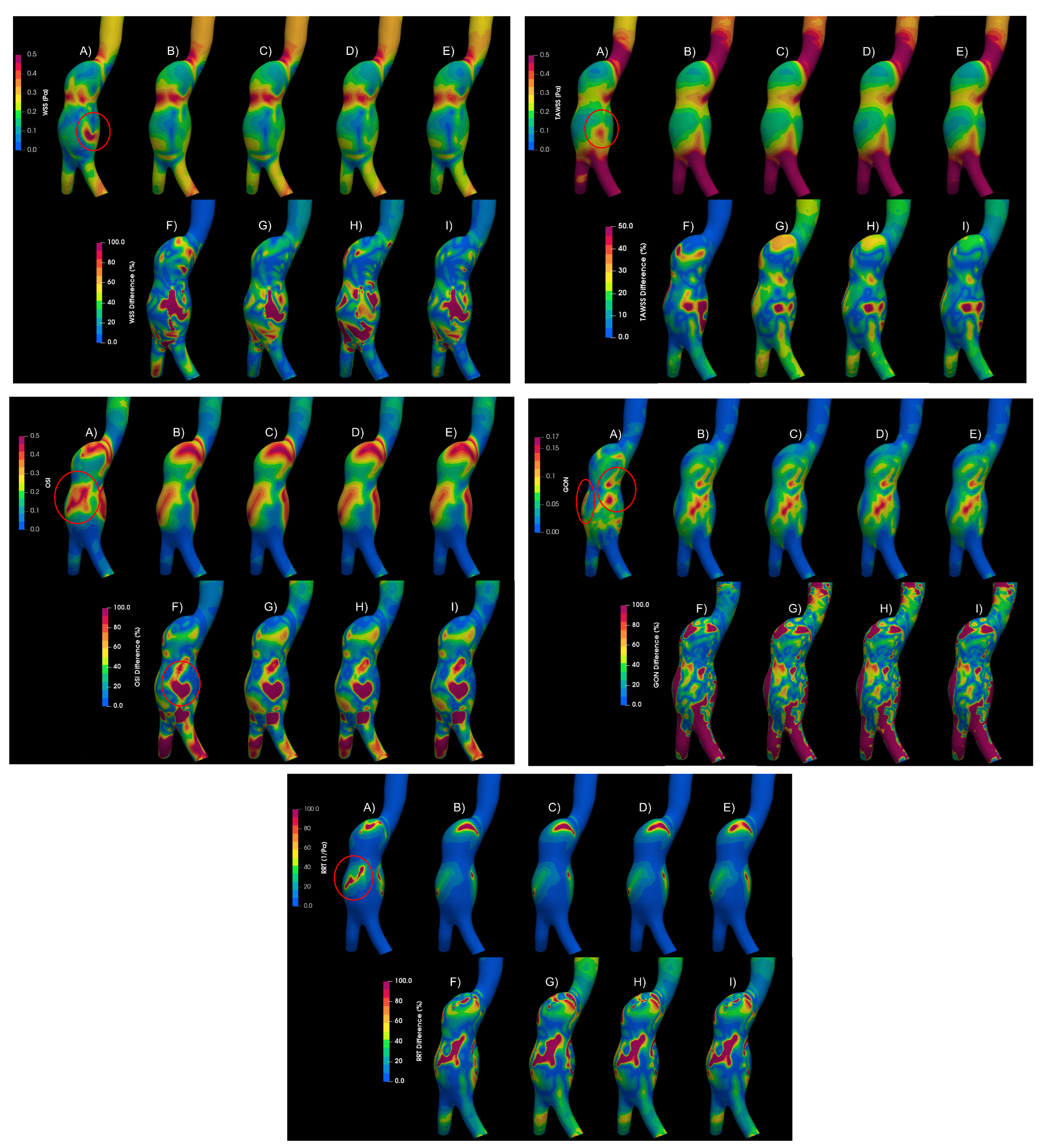
Figure 9.
Newtonian value of OSI at different cycles.
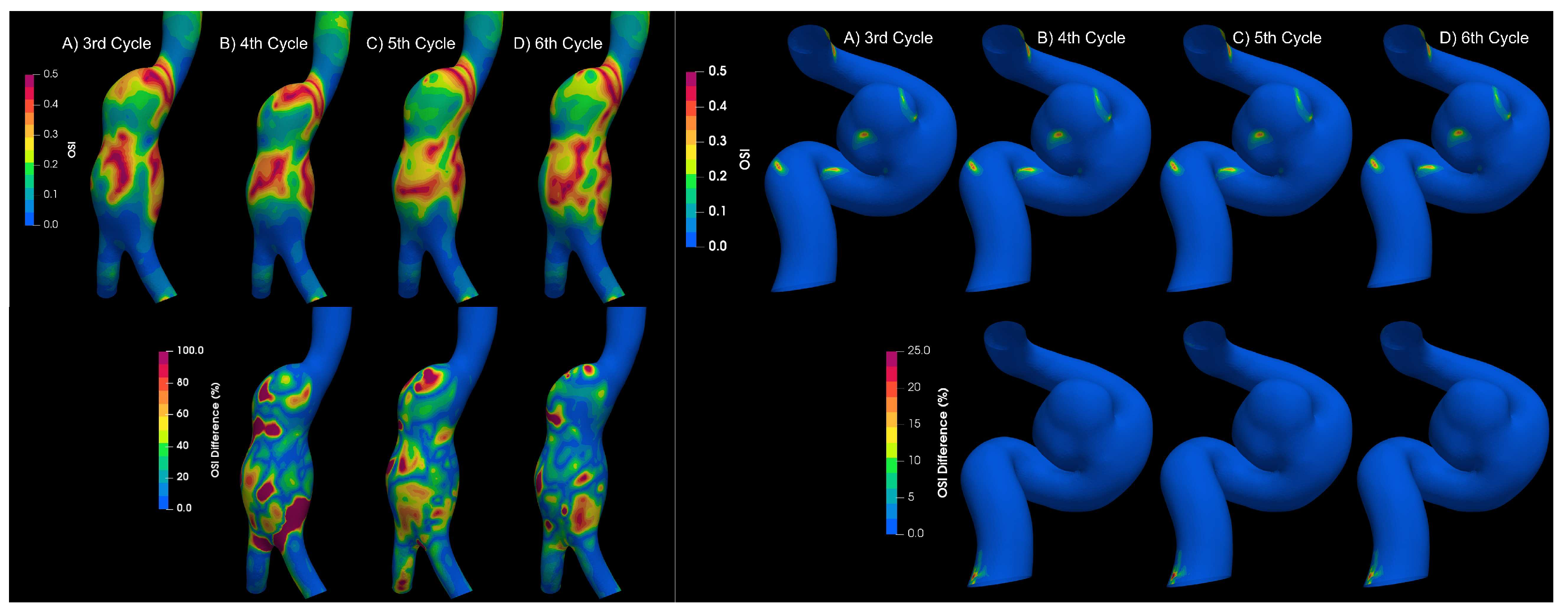
Figure 10.
Oscillatory Share Index results of Newtonian and non-Newtonian models, comparing turbulence models. A) Newtonian laminar B) Newtonian KE C) Carreau KE D) Casson KE E)Power-Law-KE F) Newtoanian laminar-Newtonian KE Differences G) Newtoanian laminar-Carreau KE Differences H) Newtoanian laminar-Casson KE Differences I) Newtoanian laminar-PowerLaw KE Differences
3.3. Fluid-Solid Interaction (FSI)
The movement of the elastic arterial wall under the effects of the pulsatile signal results in a different fluid dynamics behaviour in comparison to the consideration of a rigid wall. All the indices analyzed present different patterns, the one that presented the greatest difference with respect to these two considerations of the wall was the GON, where the patterns are completely different and the average of the differences in the entire area of the aneurysm is 43%, while the next index that had the greatest difference was the WSS during diastole with 25%, the third place is occupied by the index most related to intracranial aneurysms, the OSI, with a 20% difference, Figure 11.
The results of all cases are shown in the repository [28].
4. Discussion
Laminar and turbulent flow models were compared using four rheological models and rigid or elastic walls to simulate the flow in two aortic aneurysms and a intracranial aneurysm. According to Pratumwal et al., [33], the Carreau model is the best to describe the blood rheology; however, for IA the rheology has little influence on the flow behaviour. Meanwhile, for AAA the biggest differences are presented by the Carreau model with respect to the Newtonian model, for WSS (25%) and TAWSS (22%), Figure 12. For RRT the effect of the rheological model is greater than the laminar-turbulent flow, Figure 13.
No differences were found between laminar and turbulent flows for WSS and TWSS. Turbulent model underestimate the OSI, RRT, and GON in comparison with the laminar flow. Therefore, it is of great relevance the flow model to simulate the blood flow in aortic aneurysms. Finally, the most relevant effect to take into consideration for numerical simulations is the rigid-elastic wall assumption.
Author Contributions
Conceptualization, C.E. and F.M.; methodology, C.E. and A. B.; software, B.H. and A.B.; validation, G.M., A.B. and C.E.; formal analysis, J.N., A.G., A.B. and C.E.; investigation, A.B., F.M., and C.E.; resources, B.H. and J.N.;; writing—original draft preparation, C.E. and A.B.; writing—review and editing, C.E., F.M., B.H; project administration, C.E.; funding acquisition, C.E. and J.N. All authors have read and agreed to the published version of the manuscript.
Funding
This research was supported by Consejo Nacional de Humanidades, Ciencias y Tecnologías (CONAHCYT), grant number 728924.” and “This research was funded by Consejo Nacional de Humanidades, Ciencias y Tecnologías, grant Ciencia de Frontera 2019 CF-2019-6358.
Informed Consent Statement
“Not applicable”.
Data Availability Statement
The data presented in this study are openly available in Mendeley Data at [ doi: 10.17632/rhvvbxwwh4.2].
Acknowledgments
The authors gratefully acknowledge the computing time granted by LANCAD on the supercomputer Miztli at DGTIC UNAM. Project LANCAD-UNAM-DGTIC-404. This research used resources of the Oak Ridge Leadership Computing Facility, which is a DOE Office of Science User Facility supported under Contract DE-AC05-00OR22725.
Conflicts of Interest
“The authors declare no conflict of interest.”.
Abbreviations
| FSI | Fluid-structure interaction |
| OSI | Oscillatory shear index |
| GON | Gradient oscillatory number |
| CFD | Computational fluid dynamic |
| AAA | Aortic Aneurysms |
| IA | Intracranial Aneurysm |
| WSS | Wall shear stresss |
| TAWSS | Time Average Wall Shear Stress |
| RRT | Relative Residence Time |
| DSA | Digital Substraction Angiography |
References
- Alam, M.; Mut, F.; Cebral, J.R.; Seshaiyer, P. Quantification of the Rupture Potential of Patient-Specific Intracranial Aneurysms under Contact Constraints. Bioengineering 2021, 8. [Google Scholar] [CrossRef]
- Le Bras, A.; Boustia, F.; Janot, K.; Le Pabic, E.; Ouvrard, M.; Fougerou-Leurent, C.; Ferre, J.C.; Gauvrit, J.Y.; Eugene, F. Rehearsals using patient-specific 3D-printed aneurysm models for simulation of endovascular embolization of complex intracranial aneurysms: 3D SIM study. Journal of Neuroradiology 2023, 50, 86–92. [Google Scholar] [CrossRef]
- Epshtein, M.; Korin, N. Mapping the Transport Kinetics of Molecules and Particles in Idealized Intracranial Side Aneurysms. Scientific Reports 2018, 8. [Google Scholar] [CrossRef]
- Sheikh, M.A.A.; Shuib, A.S.; Mohyi, M.H.H. A review of hemodynamic parameters in cerebral aneurysm. Interdisciplinary Neurosurgery 2020, 22, 100716. [Google Scholar] [CrossRef]
- Longo, M.; Granata, F.; Racchiusa, S.; Mormina, E.; Grasso, G.; Longo, G.M.; Garufi, G.; Salpietro, F.M.; Alafaci, C. Role of Hemodynamic Forces in Unruptured Intracranial Aneurysms: An Overview of a Complex Scenario. World Neurosurgery 2017, 105, 632–642. [Google Scholar] [CrossRef] [PubMed]
- Carty, G.; Chatpun, S.; Espino, D.M. Modeling Blood Flow Through Intracranial Aneurysms: A Comparison of Newtonian and Non-Newtonian Viscosity. Journal of Medical and Biological Engineering 2016, 36, 396–409. [Google Scholar] [CrossRef]
- Lee, C.; Zhang, Y.; Takao, H.; Murayama, Y.; Qian, Y. A fluid–structure interaction study using patient-specific ruptured and unruptured aneurysm: The effect of aneurysm morphology, hypertension and elasticity. Journal of Biomechanics 2013, 46, 2402–2410. [Google Scholar] [CrossRef] [PubMed]
- Han, S.; Schirmer, C.M.; Modarres-Sadeghi, Y. A reduced-order model of a patient-specific cerebral aneurysm for rapid evaluation and treatment planning. Journal of Biomechanics 2020, 103, 109653. [Google Scholar] [CrossRef]
- Poelma, C.; Watton, P.N.; Ventikos, Y. Transitional flow in aneurysms and the computation of haemodynamic parameters. Journal of the Royal Society Interface 2015, 12. [Google Scholar] [CrossRef]
- Moradicheghamahi, J.; Sadeghiseraji, J.; Jahangiri, M. Numerical solution of the Pulsatile, non-Newtonian and turbulent blood flow in a patient specific elastic carotid artery. International Journal of Mechanical Sciences 2019, 150, 393–403. [Google Scholar] [CrossRef]
- Ascolese, M.; Farina, A.; Fasano, A. The Fåhræus-Lindqvist effect in small blood vessels: how does it help the heart? Journal of Biological Physics 2019, 45, 379–394. [Google Scholar] [CrossRef] [PubMed]
- Abbasian, M.; Shams, M.; Valizadeh, Z.; Moshfegh, A.; Javadzadegan, A.; Cheng, S. Effects of different non-Newtonian models on unsteady blood flow hemodynamics in patient-specific arterial models with in-vivo validation. Computer Methods and Programs in Biomedicine 2020, 186, 105185. [Google Scholar] [CrossRef] [PubMed]
- Abugattas, C.; Aguirre, A.; Castillo, E.; Cruchaga, M. Numerical study of bifurcation blood flows using three different non-Newtonian constitutive models. Applied Mathematical Modelling 2020, 88, 529–549. [Google Scholar] [CrossRef]
- Fukazawa, K.; Ishida, F.; Umeda, Y.; Miura, Y.; Shimosaka, S.; Matsushima, S.; Taki, W.; Suzuki, H. Using Computational Fluid Dynamics Analysis to Characterize Local Hemodynamic Features of Middle Cerebral Artery Aneurysm Rupture Points. World Neurosurgery 2015, 83, 80–86. [Google Scholar] [CrossRef] [PubMed]
- Qiu, Y.; Wang, J.; Zhao, J.; Wang, T.; Zheng, T.; Yuan, D. Association Between Blood Flow Pattern and Rupture Risk of Abdominal Aortic Aneurysm Based on Computational Fluid Dynamics. European Journal of Vascular and Endovascular Surgery 2022, 64, 155–164. [Google Scholar] [CrossRef] [PubMed]
- Perdikaris, P.; Insley, J.A.; Grinberg, L.; Yu, Y.; Papka, M.E.; Karniadakis, G.E. Visualizing multiphysics, fluid-structure interaction phenomena in intracranial aneurysms. Parallel Computing 2016, 55, 9–16. [Google Scholar] [CrossRef]
- Wang, X.; Li, X. Computational simulation of aortic aneurysm using FSI method: Influence of blood viscosity on aneurismal dynamic behaviors. Computers in Biology and Medicine 2011, 41, 812–821. [Google Scholar] [CrossRef]
- Jiang, Y.; Lu, G.; Ge, L.; Huang, L.; Wan, H.; Wan, J.; Zhang, X. Rupture point hemodynamics of intracranial aneurysms: Case report and literature review. Annals of Vascular Surgery - Brief Reports and Innovations 2021, 1, 100022. [Google Scholar] [CrossRef]
- 2023.
- Bilgi, C.; Atalik, K. Numerical investigation of the effects ofblood rheology and wall elasticity in abdominal aortic aneurysm under pulsatile flow conditions. Biorheology 2019, 56, 51–71. [Google Scholar] [CrossRef]
- Kim, S.; Cho, Y.I.; Jeon, A.H.; Hogenauer, B.; Kensey, K.R. A new method for blood viscosity measurement. Journal of Non-Newtonian Fluid Mechanics 2000, 94, 47–56. [Google Scholar] [CrossRef]
- Carvalho, M.V.P.; Lobosco, R.J.; Júnior, G.B.L. Rheological Analysis of Blood Flow in the Bifurcation of Carotid Artery with OpenFOAM. Proceedings of the 4th Brazilian Technology Symposium (BTSym’18); Iano, Y., Arthur, R., Saotome, O., Vieira Estrela, V., Loschi, H.J., Eds.; Springer International Publishing: Cham, 2019; pp. 223–230. [Google Scholar]
- Johnston, B.M.; Johnston, P.R.; Corney, S.; Kilpatrick, D. Non-Newtonian blood flow in human right coronary arteries: Steady state simulations. Journal of Biomechanics 2004, 37, 709–720. [Google Scholar] [CrossRef] [PubMed]
- Bazilevs, Y.; Hsu, M.C.; Zhang, Y.; Wang, W.; Kvamsdal, T.; Hentschel, S.; Isaksen, J.G. Computational vascular fluid-structure interaction: Methodology and application to cerebral aneurysms. Biomechanics and Modeling in Mechanobiology 2010, 9, 481–498. [Google Scholar] [CrossRef] [PubMed]
- Torii, R.; Oshima, M.; Kobayashi, T.; Takagi, K.; Tezduyar, T.E. Fluid-structure interaction modeling of a patient-specific cerebral aneurysm: Influence of structural modeling. Computational Mechanics 2008, 43, 151–159. [Google Scholar] [CrossRef]
- Isaksen, J.G.; Bazilevs, Y.; Kvamsdal, T.; Zhang, Y.; Kaspersen, J.H.; Waterloo, K.; Romner, B.; Ingebrigtsen, T. Determination of wall tension in cerebral artery aneurysms by numerical simulation. Stroke 2008, 39, 3172–3178. [Google Scholar] [CrossRef]
- Banerjee, M.K.; Ganguly, R.; Datta, A. Effect of Pulsatile Flow Waveform and Womersley Number on the Flow in Stenosed Arterial Geometry. ISRN Biomathematics 2012, 2012, 1–17. [Google Scholar] [CrossRef]
- Escobar-del Pozo, Carlos. Aneurysms flow numerical simulation CFD - Evaluation of rheological models, 2021. [CrossRef]
- Munarriz, Pablo. ; Gómez, P.A.; Paredes, I.; Castaño-Leon, A.M.; Cepeda, S.; Lagares, A. Basic Principles of Hemodynamics and Cerebral Aneurysms. World Neurosurgery 2016, 88, 311–319. [Google Scholar] [CrossRef]
- Meng, H.; Tutino, V.; Xiang, J.; Siddiqui, A. High WSS or Low WSS? Complex interactions of hemodynamics with intracranial aneurysm initiation, growth, and rupture: Toward a unifying hypothesis. American Journal of Neuroradiology 2014, 35, 1254–1262. [Google Scholar] [CrossRef]
- Hershey, D.; Im, C.S. Critical reynolds number for sinusoidal flow of water in rigid tubes. AIChE Journal 1968, 14, 807–809. [Google Scholar] [CrossRef]
- NEREM, R.M.; SEED, W.A. An in vivo study of aortic flow disturbances 1972.
- Yotsakorn Pratumwal.; Wiroj Limtrakarn.; Sombat Muengtaweepongsa.; Phatsawadee Phakdeesan.; Suttirak Duangburong.; Patipath Eiamaram.; Kannakorn Intharakham. Whole blood viscosity modeling using power law, Casson, and Carreau Yasuda models integrated with image scanningU-tube viscometer technique. Songklanakarin Journal of Science and Technology (SJST) 2017, 39, 5. [CrossRef]
Figure 1.
Test mesh independence of the area-averaged WSS as a function of time for the whole surface for all cases.
Figure 1.
Test mesh independence of the area-averaged WSS as a function of time for the whole surface for all cases.
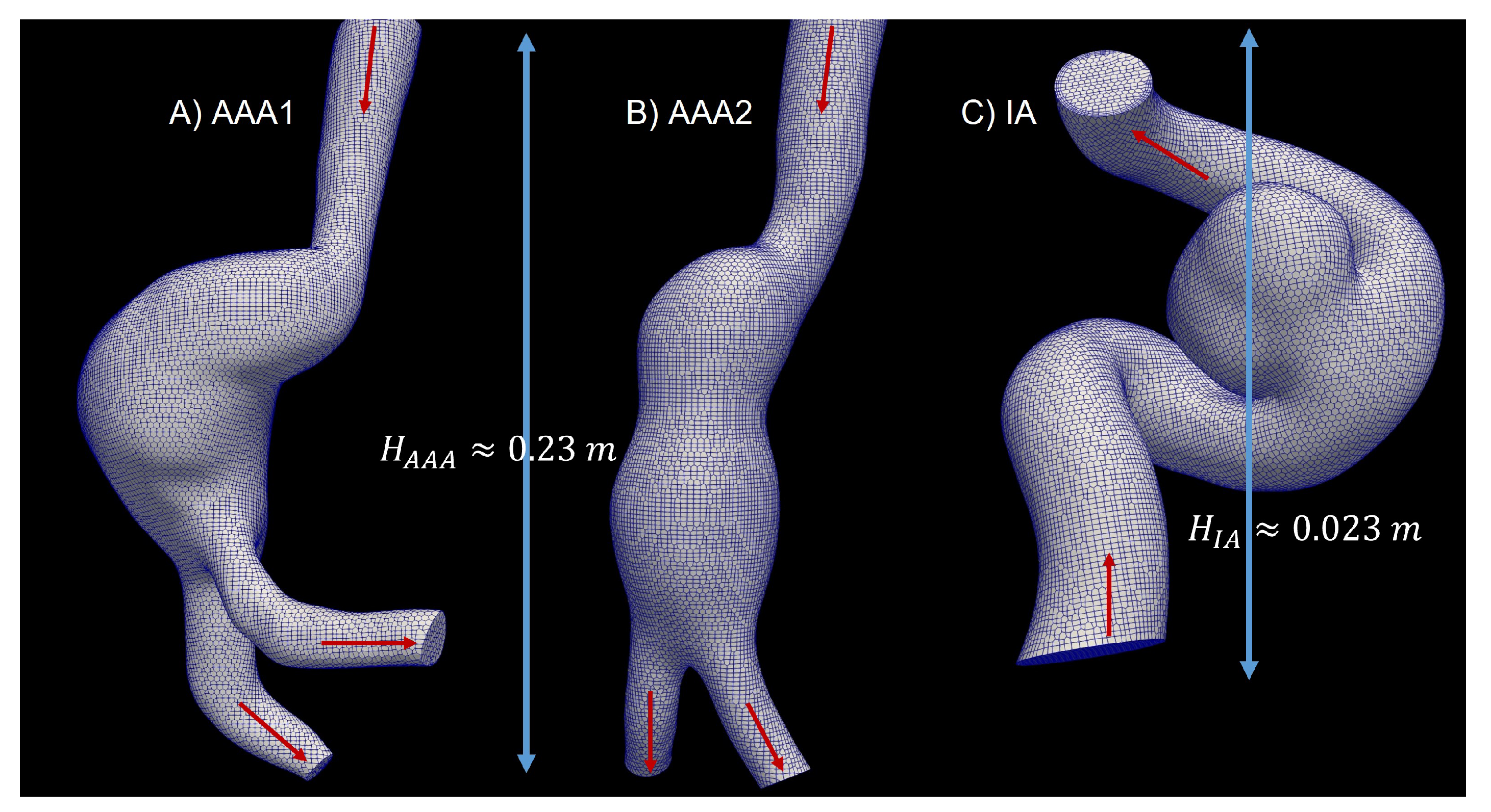
Figure 2.
Test mesh independence of the area-averaged WSS as a function of time for the whole surface for all cases.
Figure 2.
Test mesh independence of the area-averaged WSS as a function of time for the whole surface for all cases.
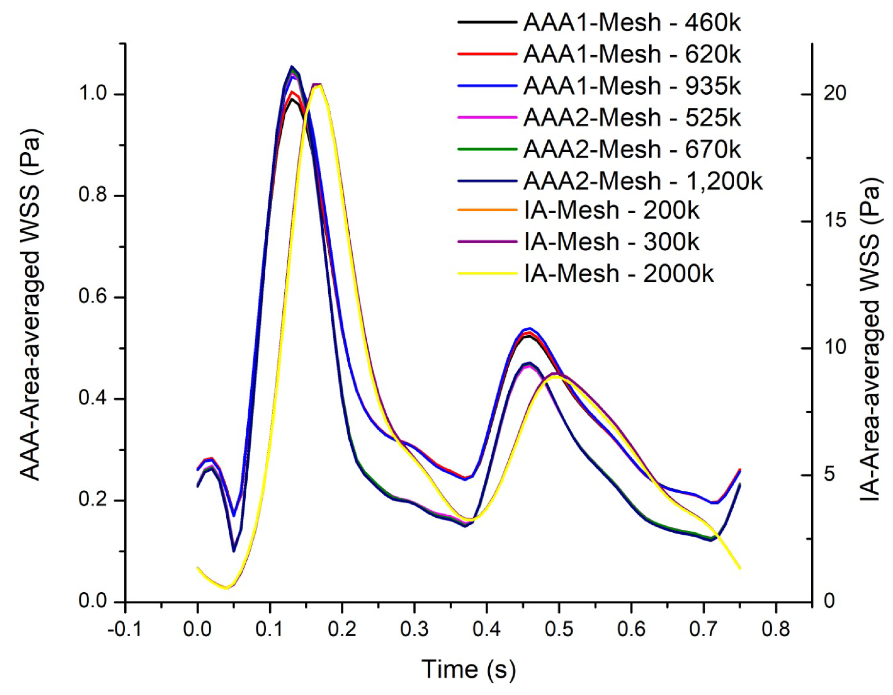
Figure 3.
Hemodynamic indices studied in IA. A) WSS in peak Diastole, B) WSS in peak systole C) Time-Area-Average WSS, D) Osillatory Share Index, E) Relative Recidence Time and F) Gradient Oscilatory Number.
Figure 3.
Hemodynamic indices studied in IA. A) WSS in peak Diastole, B) WSS in peak systole C) Time-Area-Average WSS, D) Osillatory Share Index, E) Relative Recidence Time and F) Gradient Oscilatory Number.
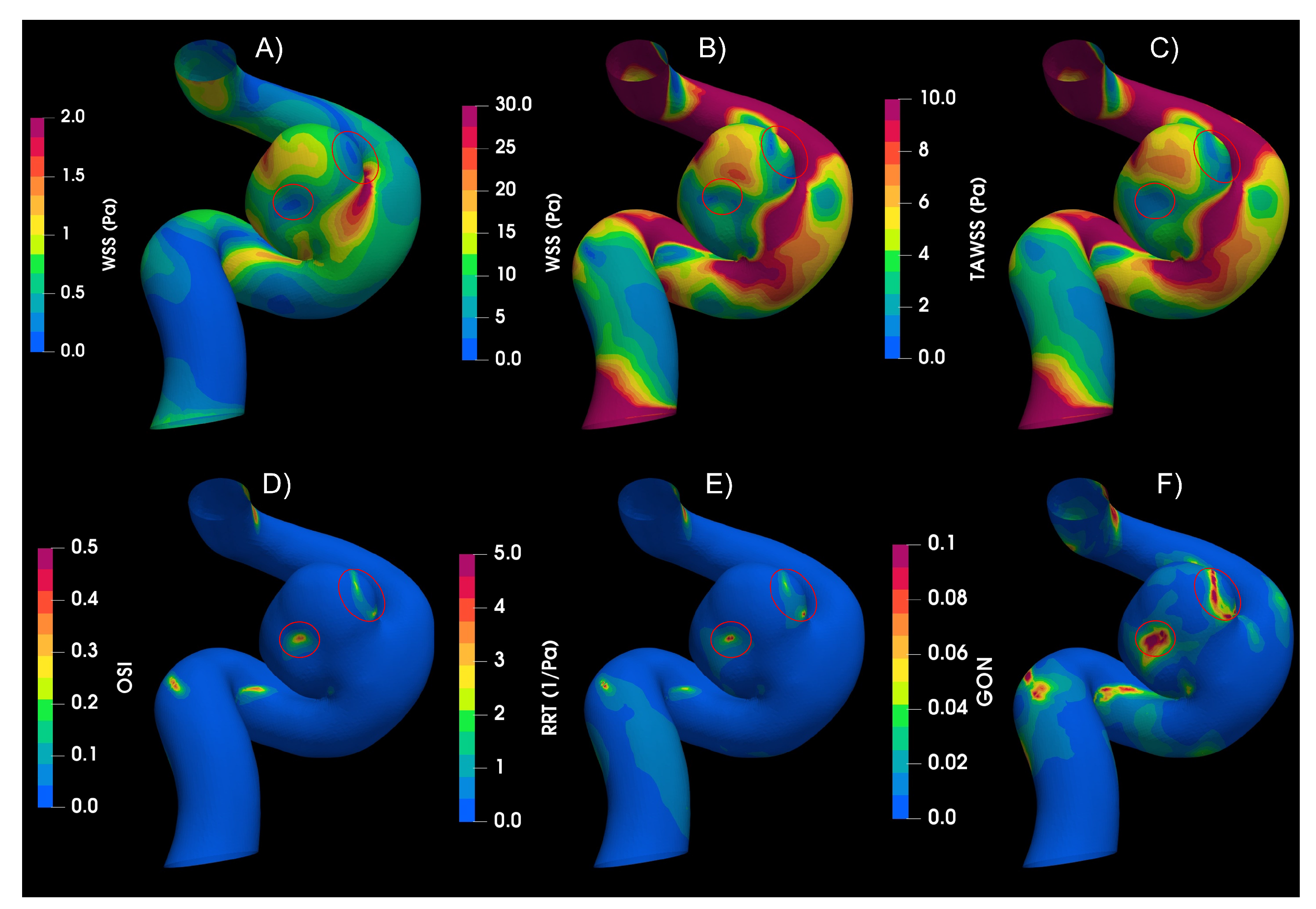
Figure 4.
Hemodynamic indices studied in AAA1. A) WSS in peak Diastole, B) WSS in peak systole C) Time-Area-Average WSS, D) Osillatory Share Index, E) Relative Recidence Time and F) Gradient Oscilatory Number.
Figure 4.
Hemodynamic indices studied in AAA1. A) WSS in peak Diastole, B) WSS in peak systole C) Time-Area-Average WSS, D) Osillatory Share Index, E) Relative Recidence Time and F) Gradient Oscilatory Number.
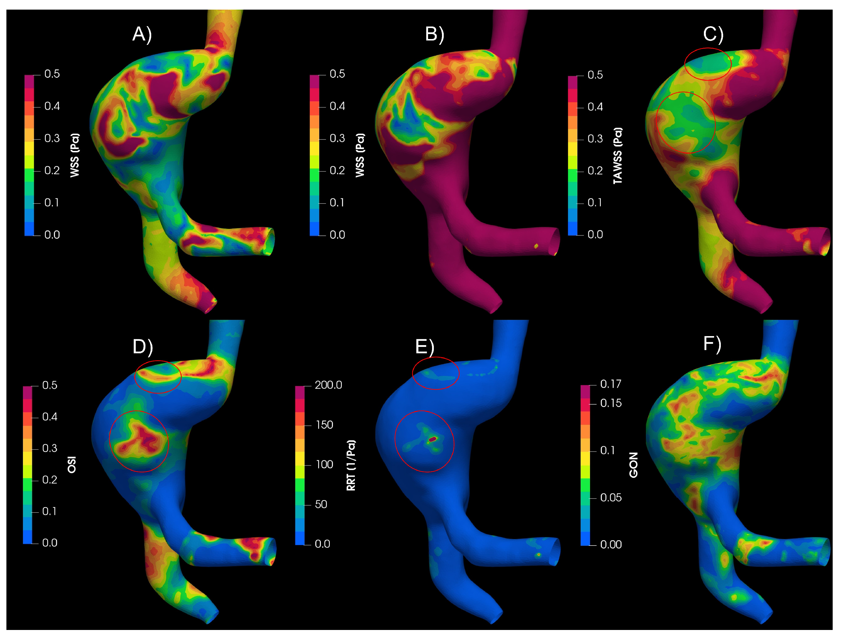
Figure 5.
Oscillatory Share Index results of Newtonian and non-Newtonian models. A) Newtonian B) Crreau C) Casson D)Power-Law E) Newtoanian-Carreau Differences F) Newtoanian-Casson Differences E) Newtoanian-PowerLaw Differences
Figure 5.
Oscillatory Share Index results of Newtonian and non-Newtonian models. A) Newtonian B) Crreau C) Casson D)Power-Law E) Newtoanian-Carreau Differences F) Newtoanian-Casson Differences E) Newtoanian-PowerLaw Differences
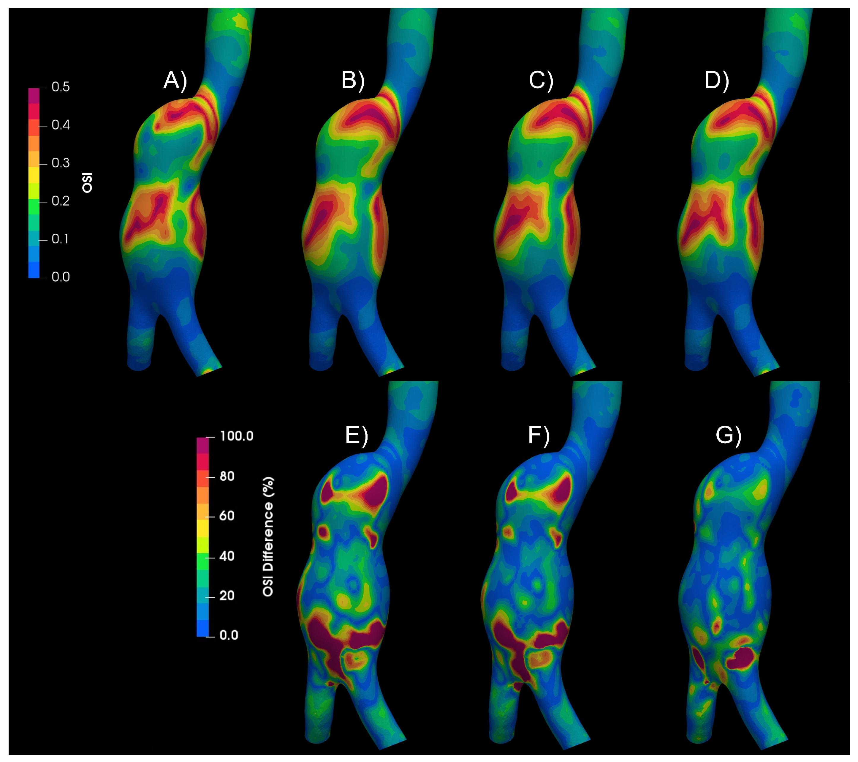
Figure 6.
Velocity plane contour. A) Plane, B) Newtonian model, C) Carreau model, D) Newtoanian-Carreau Differences.
Figure 6.
Velocity plane contour. A) Plane, B) Newtonian model, C) Carreau model, D) Newtoanian-Carreau Differences.
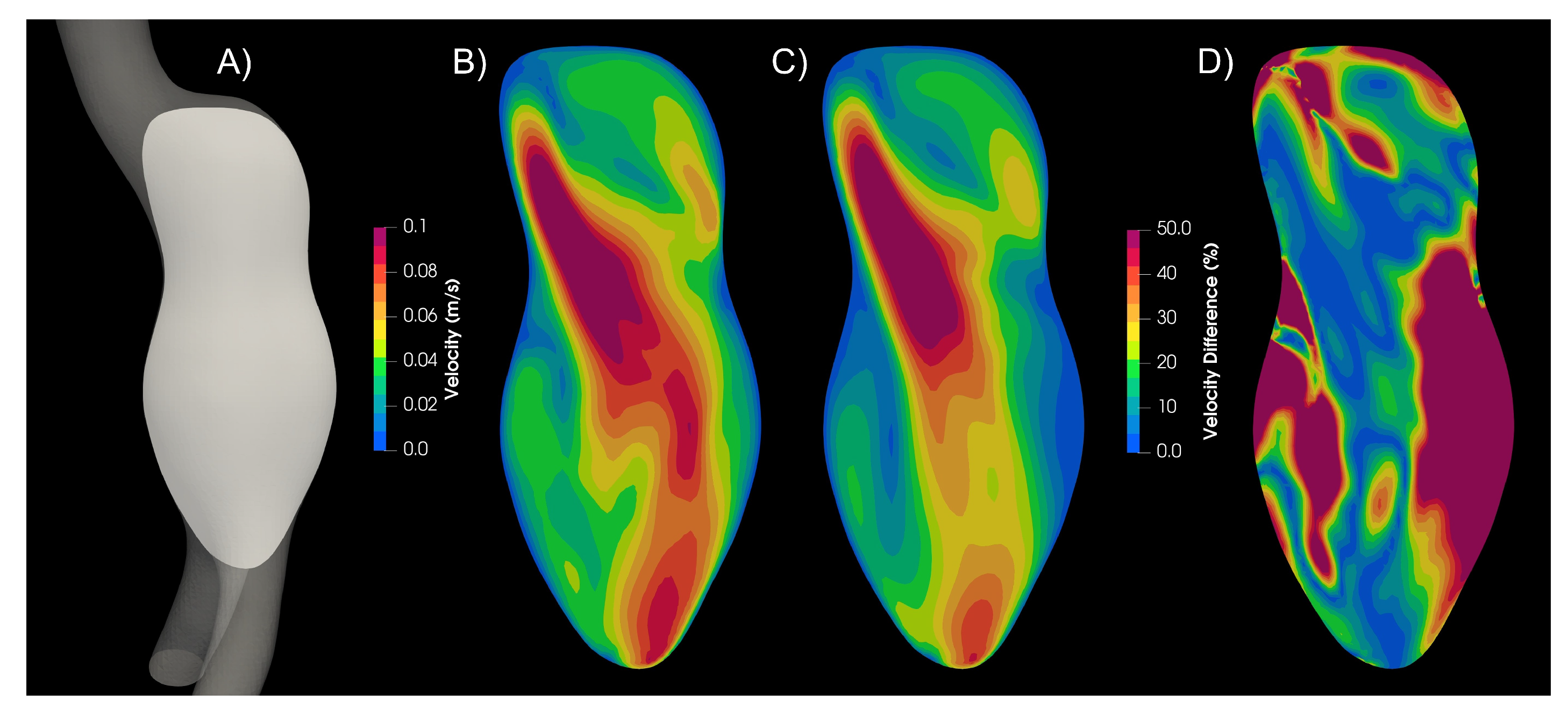
Figure 7.
OSI results for different cycles for aortic and intracranial aneurysms.
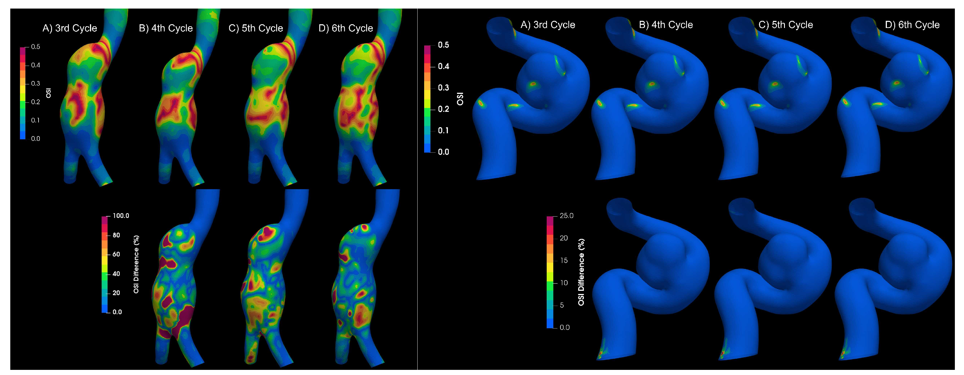
Figure 11.
Camparison of rigid and elastic wall. A) OSI values of rigid, laminar and newtonian case. B) OSI values of elastic, laminar and newtonian case. C) OSI Differences between rigid and elastic wall. D) TAWSS values of rigid, laminar and newtonian case. E) TAWSS values of elastic, laminar and newtonian case. F) TAWSS Differences between rigid and elastic wall.
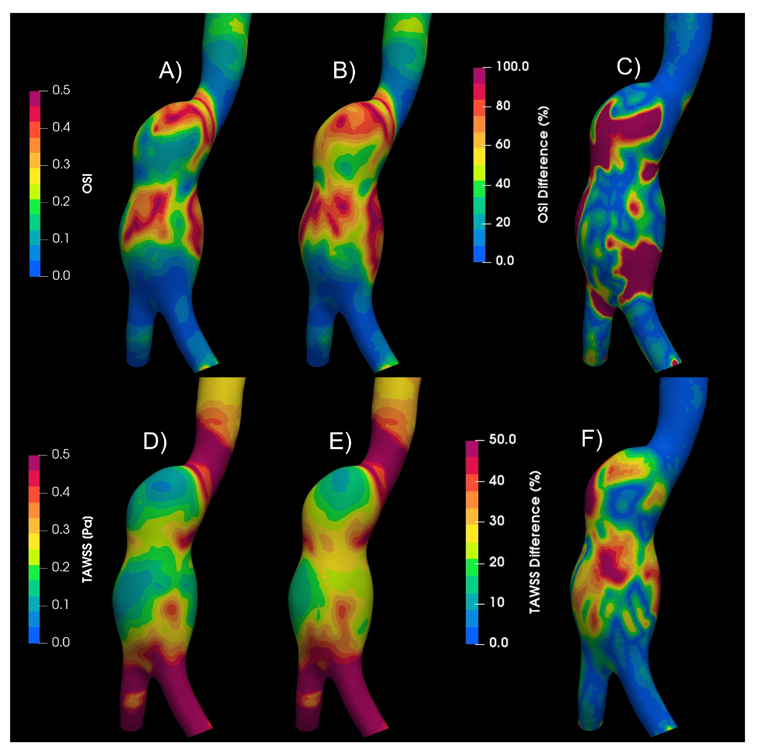
Figure 12.
Area average WSS in peak diastole, peak systole, TAWSS, and OSI area average results in AAA2 under reological, turbulence and elastic models studied.
Figure 12.
Area average WSS in peak diastole, peak systole, TAWSS, and OSI area average results in AAA2 under reological, turbulence and elastic models studied.
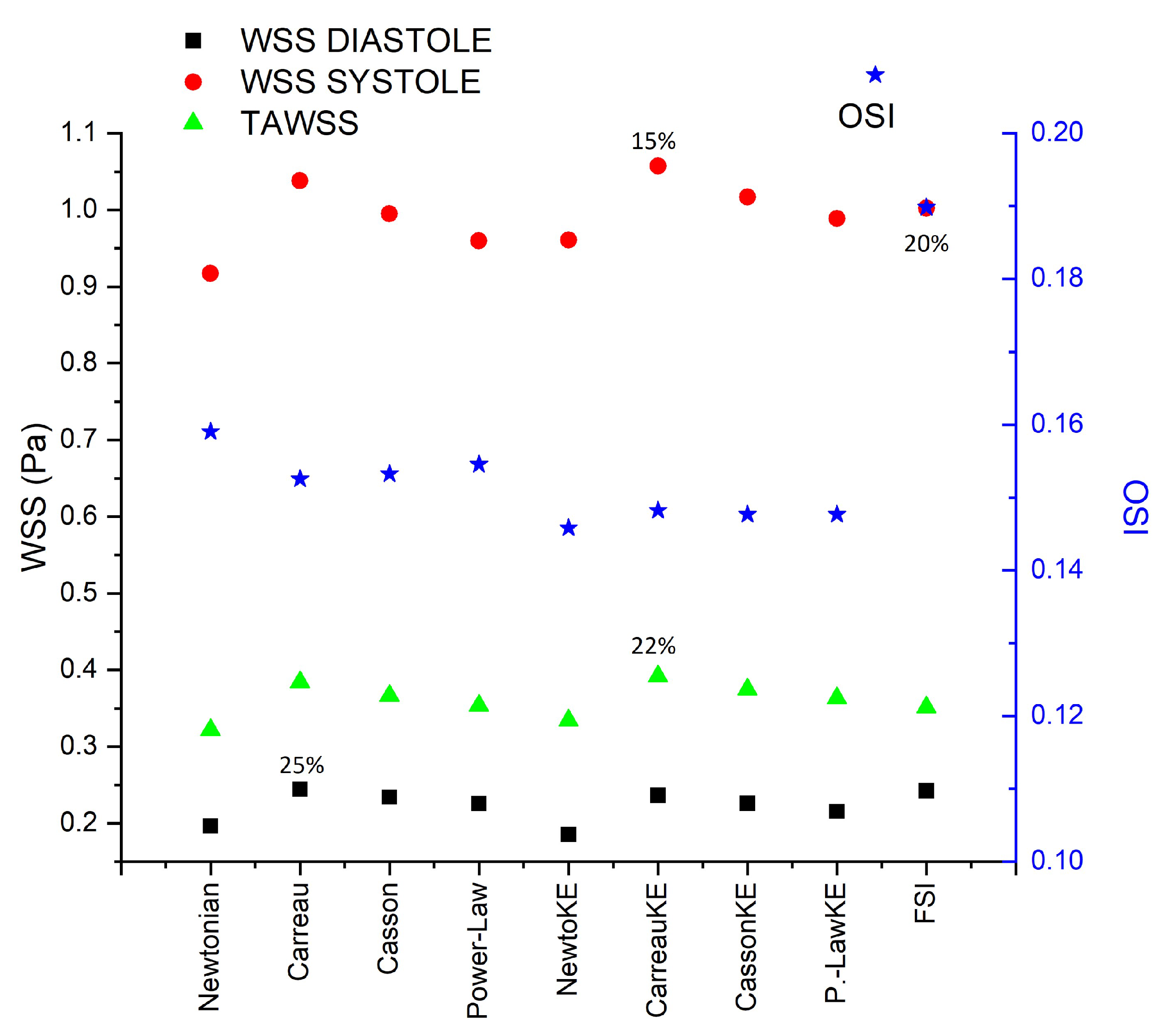
Figure 13.
RRT and GON area average results in AAA2 under reological, turbulence and elastic models studied.
Figure 13.
RRT and GON area average results in AAA2 under reological, turbulence and elastic models studied.

Table 1.
Effective viscosity equations of various models with their parameters.
| MODEL | PARAMETERS | |
|---|---|---|
| Newtonian | Pa.s | [20] |
| Power-law | , | [21] |
| Casson | Pa.s , Pa | [22] |
| Carreau |
Pa.s, s Pa.s, |
[23] |
Table 2.
Strain Rate in all models.
| Strain Rate | AAA1 | AAA2 | IA |
|---|---|---|---|
| Artery Wall | 125 | 97 | 1888 |
| Aneurysm Wall | 89 | 73 | 1480 |
| Artery Body | 19 | 22 | 502 |
| Aneurysm Body | 15 | 20 | 388 |
Disclaimer/Publisher’s Note: The statements, opinions and data contained in all publications are solely those of the individual author(s) and contributor(s) and not of MDPI and/or the editor(s). MDPI and/or the editor(s) disclaim responsibility for any injury to people or property resulting from any ideas, methods, instructions or products referred to in the content. |
© 2023 by the authors. Licensee MDPI, Basel, Switzerland. This article is an open access article distributed under the terms and conditions of the Creative Commons Attribution (CC BY) license (http://creativecommons.org/licenses/by/4.0/).
Copyright: This open access article is published under a Creative Commons CC BY 4.0 license, which permit the free download, distribution, and reuse, provided that the author and preprint are cited in any reuse.


