
Submitted:
16 August 2023
Posted:
17 August 2023
You are already at the latest version
Abstract
Barrier coverage is a fundamental application in wireless sensor networks, which is widely used to protect a region through intruder detection for smart city. In this paper, we study a new branch of barrier coverage, named warning barrier coverage (WBC). Different from the classic barrier coverage, WBC has the inverse protect direction, which protects unexpected visitors by warning them away from the region enclosed by sensor barriers. The WBC holds a promising prospect in many danger keep out applications for smart city. For example, a WBC can enclose the debris area in the sea and alarm any approaching ships in order to avoid their damaging propellers. One special feature of WBC is that the target region is usually dangerous and its boundary is previously unknown. Hence, the scattered mobile nodes need to detect the boundary and form the barrier coverage themselves. It is challenging to form these distributed sensor nodes into a barrier because a node can sense only the local information and there is no global information of the unknown region or other nodes. To this end, we propose a novel solution AutoBar for mobile sensor nodes to automatically form a WBC for smart city. To pursue the high coverage quality, we theoretically derive the optimal distribution pattern of sensor nodes using convex theory. Based on the analysis, we design a fully distributed algorithm that enables nodes to collaboratively move towards the optimal distribution pattern. In addition, AutoBar is able to reorganize the barrier even any node is broken. To validate the feasibility of AutoBar, we develop the prototype of the specialized mobile node, which consists of two kinds of sensors: one for boundary detection and another for visitor detection. Based on the prototype, we conduct extensive real trace driven simulations in various smart city scenarios. Performance results demonstrate that AutoBar outperforms the existing barrier coverage strategies in terms of coverage quality, formation duration, and communication overhead.
Keywords:
barrier coverage
; mobile sensor networks
; boundary detection
; convex analysis
; virtual force
1. Introduction
Barrier coverage [15] is one vital application in wireless sensor networks (WSNs) for smart city [2,27], which forms sensor nodes surrounding into barriers to protect a region by detecting all intruders. A wide range of safety scenarios of smart city demand barrier coverage, for example, the country border surveillance for stowaway detection. In this paper, we extend the classic concept of barrier coverage to a new branch, which moves the sensor nodes surrounding a dangerous region and protects any unexpected visitors by warning them away from the dangers, so-called warning barrier coverage (WBC). The WBC is promising in many danger keep out application for smart city. For example, a WBC can surround debris areas in floods and alarm rescue workers to avoid unnecessary harms. Moreover, WBC can warn people to avoid entering dangerous areas such as hazardous gas leaks and even nuclear radiations in cities.
We compare the classic barrier coverage and WBC in Table 1. Different from the classic barrier coverage, WBC focuses on the danger keep out applications whose boundary of target region is previously unknown. To avoid danger, people cannot get close to the region or deploy sensor nodes manually. Hence, besides the visitor detection, sensor nodes in WBC should have the capability to detect the boundary as well. Based on the sensing results, mobile sensor nodes form the barrier collaboratively.
Regardless of the classic barrier coverage used in WBC, the formation process [21] is crucial because newly deployed sensor nodes lack a dependable infrastructure for communication and detection. The formation process in WBC is defined to form sensor nodes into k barriers enclosing the region, thus detecting or warning unexpected visitors.
Researchers have put forward various solutions in the literature for classic barrier coverage formation for smart city. For instance, Kumar [15] proposed a centralized algorithm to determine weak k-barrier coverage in a region using randomly deployed sensor networks. Later, [18] devised efficient algorithms to construct strong sensor barriers. And [22] studied the barrier coverage of line-based deployment. In addition, [32] finded a cluster-based barrier construction algorithm in mobile Wireless Sensor Networks.
Different from the known region in classic barrier coverage, the boundary of a dangerous region in WBC is usually unknown. Hence, the classic formation approaches are not appropriate for WBC in smart city. In addition, most existing works [15,22] fall into the category that forms the barrier coverage by stationary sensor nodes. Nevertheless, if the stationary sensor nodes are stochastically deployed, many redundant nodes will be needed to ensure a strong barrier [18]. On the other hand, if the stationary nodes are manually deployed, a lot of manpower and time are consumed. Especially, in some cases for smart city, the region is quite large in scale or hides dangers. Therefore, using stationary nodes is more of a hindrance than a help in WBC. A few state-of-the-art works also considered using mobile sensor nodes [16,33,34] to facilitate the barrier coverage. However, these works assumed that the region boundary is pre-known [23], which is not practical in WBC.
To tackle the formation problem in WBC, in this paper, we propose a distributed movement strategy for mobile nodes to form the barrier coverage automatically for smart city. The basic objective of the proposed strategy is to leverage the given number of mobile nodes to form a barrier coverage with the highest coverage quality, i.e., the maximal k-barrier coverage [15]. However, in scenarios where sensor nodes lack prior knowledge of their initial positions or the boundaries of the region, their movement can only be determined based on the local information they sense and communicate. This practical challenge presents a significant design obstacle.
In order to address the challenge, we study the barrier coverage formation problem as follows: First, based on the convex analysis [20], we derive: the optimal distribution pattern for k-barrier coverage is that all sensor nodes are evenly distributed on the convex hull of the region. Second, we devise an algorithm AutoBar, which navigates the sensor nodes to detect the region boundary by themselves and then gradually move approaching the optimal distribution pattern based on their local information. Third, extensive simulations verify the validity of AutoBar and evaluate its characteristics such as formation duration, communication overhead, and moving distance.
In summary, the major contributions of this paper are as follows:
- As far as we know, this is the first work to trigger the coverage problem of the alarm barrier for smart city, where the regional information is not pre-known.
- The optimal distribution of sensor nodes with maximum k- barrier coverage is derived to guide design.
- A fully distributed algorithm is developed to automatically form barrier coverage for sensor nodes.
The rest of the paper is organized as follows: Section 2 presents the related work. Section 3 formulates the barrier coverage formation problem. Section 4 investigates the optimal distribution pattern. The proposed algorithm is designed in Section 5 and the practical issues are discussed in Section 6. Section 7 depicts the results of simulation. In Section 8, we present conclusion and future work.
2. Related Work
The coverage related problem [5,7] is a fundamental topic in WSNs to measure the monitoring quality of a sensor network deployed in a given region. Diverse directions are excellently studied for coverage problems, such as barrier coverage [15], sweep coverage [17], surface coverage [14], and trap coverage [3].
In these directions, barrier coverage is one valuable and practical application for smart city, which is advocated in [15] for the purpose of intrusion detection in country border, critical infrastructure protection, and battlefield perimeter surveillance. The barrier coverage formed by stationary nodes has been widely studied. For instance, minimum cost for achieving k-barrier coverage is calculated in [6]. In [18], strong sensor barriers were devised. Line-based and curve-based barrier coverage were studied by [22] and [9], respectively. Multi-round sensor deployment for guaranteed barrier coverage is proposed in [26]. Nevertheless, lots of resources such as redundant nodes in stochastic deployment and manpower cost in manual deployment will be needed due to the reliance on stationary nodes only.
Mobile nodes for barrier coverage was firstly introduced in [21], in which the nodes with limited mobility (e.g., one-step move with one chance) are utilized to improve the quality of barrier coverage. With the rapid development of autonomous robot technology, sensor nodes with strong mobility [11] become practical. In addition, a movement barrier formation algorithm MobiBar was designed in [23]. presented distributed algorithms for barrier coverage using sensor relocation. [30] proposed a heuristic target-barrier construction algorithm to solve the target-barrier coverage problem while satisfying the boundary constraint conditions. These works mainly focus on centralized analysis, which is not suitable for large-scale barrier coverage for smart city.
Distributed algorithms for mobile barrier coverage were also investigated in the literature. The chain reaction algorithm [13] was firstly developed for mobile barrier formation. But it totally ignores the situation of node failure, which would lead to certain loopholes in the barrier. Based on mobility and intruder prior information, PMS [8] is able to improve the quality of barrier coverage. However, PMS assumes that the region knowledge is pre-known, which is not practical in most real WBC applications of smart city. Besides, [31] presented a distributed cellular automaton based algorithm for autonomous deployment of mobile sensors. The limitation is that the number of sensors it needs to be deployed in a fixed manner.
Thus, it is essential to design a distributed, fault-tolerant, and automatic barrier coverage formation method using mobile nodes for WBC with the unknown regions for smart city.
3. Problem Formulation
In this section, we model the objects and then formulate the automatic barrier coverage formation problem.
3.1. System Model
Region: The region of interest A is the area needing to be surrounded by the barrier coverage. Assume that the region A is an enclosed area on a 2D plane, which has a continuous boundary in our model. We also assume that the detailed boundary information of the region A is not pre-known. The only known information is the general location of A. This is a practice-motivated assumption. For example, in a hazardous gas leakage incident of city sewage pipelines, the barrier coverage formation is strongly desired to surround the diffuse region quickly and automatically, so that any unexpected visitor can be alarmed when she enters the dangerous region. In this case, the boundary of the diffuse region is not pre-known. And we can only obtain the general location where the hazardous gas leak happens.
Node: In our model, a sensor node is denoted by , where and n is a given number. Any node can move on the plane within the maximal velocity v. A node has at least two sensors to sense the region (e.g., the debris area, the nuclear area) and the unexpected visitors (e.g., the ships, the people), respectively. The sensing area of each sensor is assumed to be the widely adopted disk model [15]. The disk radius of the sensor for region sensing is denoted by . Within , we assume that the distance from the node to the region boundary can be obtained by this sensor (e.g., camera sensor) as shown in Figure 1. In addition, the disk radius of the other sensor for visitors detection is denoted by . The communication range between nodes is . Without loss of generality, we set as the setting in [15]. Every node knows its location information by equipping it with auxiliary devices such as GPS. The autonomous robotic fish for debris monitoring [24,25] is an example of such sensor node, which can move in floods, has a camera to sense the debris, has an acoustic sensor to detect any approaching rescue workers, is equipped with GPS to know its location, and has a Zigbee module to communicate with other robotic fishes and to warn the approaching rescue workers.
Warning Barrier coverage: We use a graph to describe the warning barrier coverage as in [15]. The set V consists of the vertexes corresponding to the nodes. If the distance between any two vertexes is less than , then there is an edge between them. Strong barrier coverage [18] is described as a closed chain consisting of edges surrounding the region. Due to the mobility of nodes, this study only considers the formation of strong barrier coverage. Strong k-barrier coverage is expressed as k vertex-disjointed chains in . In another word, any unexpected visitor crosses the barriers would be detected by at least k nodes. We adopt k to measure the quality of barrier coverage in this paper. Figure 2 shows an example of a barrier coverage. Any path (e.g., the dash arrow) crossing the barrier coverage is covered by 2 nodes. Since the region A is not pre-known and the number of nodes n should be given before deployment, we practically set that n is a large enough number for barrier coverage formation to the region.
3.2. Fundamental Problem
The automatic barrier coverage formation (ABCF) problem for WBC is defined that the automatic movement of all mobile nodes to form the maximum k barrier coverage around the region of interest.
The goal of solving the ABCF problem is to maximize k under the constraints of given n nodes. This problem is non-trivial due to the following challenges: First, sensor nodes just have local information through communication and sensing. Without global information about boundary, it is difficult for nodes to know their destinations and paths. Second, it is common that some sensor nodes fail during the movement because of mechanical breakdown or depleted battery. Thus, the movement strategy should take the node failure into account. Third, centralized solutions consume heavy traffic on multi-hop transmissions, which are not appropriate to large-scale WBC for smart city. Hence, a total distributed solution is required even it is not easy.
4. Theoretical Analysis
In this section, when the region A and the number n are given, we export the maximum value k.
4.1. Different Types of k-Barrier Coverage
In order to satisfy different coverage requirements for smart city, the distribution of sensor nodes in k-barrier coverage has different types. Two typical types are as follows:
Multi-level type: All sensor nodes form several disjoint barriers [23]. Figure 3a shows that 8 nodes form a 2-barrier coverage with multi-level type for a part of region with straight boundary.
Line type: All sensor nodes form several barriers on one line [22]. Figure 3b displays that 8 nodes form a 2-barrier coverage with line type for a part of region with straight boundary.
In terms of the definition of k-barrier coverage [15], the value of k is only determined that the expected visitor is discovered by at least k nodes when it passes the barriers. In Figure 3a,b, no matter which crossing path (dash arrow) is selected, the path is always covered by two nodes. Hence, we observe that both types can provide barriers. The difference between two types is: a visitor is detected by two nodes one after another in multi-level type. By contrast, it is detected by two nodes simultaneously in line type.
The advantage of multi-level type is to early detect the expected visitor benefiting from its “width". Consequently, if the coverage requirement is to detect as early as possible, multi-level type is an excellent choice. On the contrary, the strength of line type is to form k barriers with the least number of nodes. Although two types achieve the same k in Figure 3a,b, if the straight boundary changes to be the arc boundary, in order to maintain , multi-level type needs 9 nodes in Figure 3c due to outer ring always requiring more nodes, and line type only needs 8 nodes in Figure 3d. In real scenarios for smart city, an enclosed region with arc boundary is a general case.
In this paper, the coverage requirement of the ABCF problem is to maximize k with the given n nodes. It is obvious that the barrier of line type is the better candidate than the multi-level type.
4.2. Optimal Distribution Pattern
In this subsection, we derive the optimal destinations of n nodes in line type. Additionally, denotes the length of the convex hull of region A. The method of obtaining can be found in [20]. Therefore, we have:
Theorem 1.
To achieve the maximum value of k, it is sufficient for n nodes to be evenly distributed on the convex hull of region A. The maximal value of expectation k is
Proof.
Proof of Theorem 1 Convex analysis [20] establishes that the convex hull of a 2D region is the polygon with the smallest area and shortest perimeter that encompasses it. Thus, the shortest perimeter can be expressed as . This indicates that represents the minimum length required for one barrier.
Due to an edge existing when , where is the function to get the shortest distance between two objects, the maximum distance between any two connectable vertexes is . If we connect n vertexes in a series, the total length of all these vertexes is at most .
Wrap the series of vertexes around the convex hull of region A, we have the theoretical maximal value of .
Assuming a line-type distribution of sensor nodes along the shortest perimeter, each point on the perimeter is covered by multiple nodes. The minimum number of nodes covering a point is denoted as k, which corresponds to the definition of strong k-barrier coverage in [15].
When n vertexes are evenly distributed, we have the distance between any pair of the nearest neighbors
And any point on the perimeter is covered by at least
The equality obtained in Eq. (1) confirms the sufficiency of the condition, thereby proving Theorem 1. □
5. AutoBar Design
We have investigated that the destinations of n nodes are evenly distributed on the convex hull of the region in the last section. In this section, firstly, we present how the sensor nodes move to the destinations according to the proposed AutoBar algorithm. Secondly, we analyze the reasons behind the AutoBar design.
5.1. Design Overview
We exploit a distributed algorithm, called AutoBar, for the nodes with automatic movement from their initial positions to the destinations derived in Theorem 1 with only local information. The main procedure of AutoBar includes two steps: boundary seeking and barrier forming.
Step 1: Boundary seeking. The goal of this step is to design the moving path for a node to find the region boundary. Since the sensor nodes neither pre-know their initial positions (which depends on the deployment type) nor pre-know the location of the region A (no global information), the moving path cannot be pre-planed. To automatically form the barrier coverage, sensor nodes should find the region boundary in their first step no matter where are their initial positions. All initial positions can be classified into three cases: outside, on, and inside the region boundary.
Case 1.1: Outside the boundary. A node is considered outside the boundary if its distance from A, denoted as , is greater than . Node can self-determine whether it is outside the boundary through it cannot sense any part of region A within its disk, i.e., the sensing area of does not overlap with the region A. To locate the boundary, this node is design to randomly select an initial angle and then move along the Archimedean spiral as shown in Figure 4a until it meets the boundary of region A. The spiral path used for boundary detection in [4] offers several advantages. It evenly explores all directions, minimizing the risk of overlooking the region. Additional examination of the Archimedean spiral will be presented in the next subsection.
Case 1.2: On the boundary. When , the node is on the boundary, where is the function that obtains the boundary of region A. The node can be discretionary whether it is on the boundary by sensing the part of area of that overlaps with the region A. In this case, the current distance can be sensed, and then the node moves along the shortest path to the boundary, as shown in Figure 4b.
Case 1.3: Inside the boundary. When and , the node is inside the boundary. Node can be discretionary whether it is inside the boundary by sensing area of node completely overlaps with the region A, i.e., included by A. In this case, the node can move along a straight line after randomly selecting the direction to the boundary, as shown in Figure 4c.
Step 2: Barrier forming. After finding the boundary, the goal of the second step is for nodes to move together to form the maximum k-barrier coverage. Nodes have two directions along the boundary: clockwise (Right) and counterclockwise (Left). The nearest neighbor in any direction is called a direct neighbor. The barrier formation step is only based on the transmission of position information between close neighbors, which is easy to implement, energy-efficient, and low-delayed.Due to each node itself searching for boundaries, the situation of its neighbors is uncertain. There are three other cases of direct neighbors: 0, 1, or 2 direct neighbors.
Case 2.1: No neighbor. When there are no neighbors of the node in its sensing range , it should self-move to find the other nodes to form the barrier together. We design that such node moves toward the clockwise direction, along the boundary of A, and with the velocity v until encountering the other node as shown in Figure 5a.
Case 2.2: One direct neighbor. When a node has only one direct neighbor on one certain side, a virtual repulsive force [28] is generated between and . This force leads to the node moving toward the opposite direction of and along the boundary of region A until the destination location that as shown in Figure 5b.
Case 2.3: Two direct neighbors. When node on each side has two direct neighbors and , these two neighbors will generate virtual forces. The amount of force depends on the distance and . To balance these two forces, it demands that the destination location has the uniform distance to its direct neighbors and , i.e., . Moreover, a node with its two immediate neighbors can form an internal angle, which is facing to the region. We have set a limit that the internal angle should not exceed . In Figure 5c, the internal angle is . Therefore, in order to balance the forces, the destination of is ’and the moving path is along the boundary. In Figure 5d, the inner angle is because the part of the boundary is concave. In order to balance the forces and maintain the angle constraints, node moves directly to the bourn, which is the intermediate position between and .
The pseudo-code of AutoBar is shown in Table 2, where the line 2-12 present the boundary seeking step and the line 13-28 present the barrier forming step.
5.2. Design Analysis
5.2.1. Necessity of A Distributed Algorithm
It is necessary that the proposed design can determine the movement strategy distributively because of the following reasons: First, since the communication range and the sensing range , are not infinite of smart city, any node cannot directly know the global information such as the real-time positions of all the other nodes and the boundary of region A. Second, if the nodes share their real-time positions by multi-hop transmission, the communication overhead is too high, especially when n is large. Thus, we design AutoBar, in which every node determines its movement only based on its local information.
5.2.2. Archimedean Spiral in Case 1.1
In order to realize the automatic seeking, every node determines its movement according to the Step 1. The movement strategies in Case 1.2 and 1.3 (shown in Figure 4a,b) are intuitive. Then, we discuss the moving path of the Archimedean spiral in Case 1.1.
The Archimedean spiral [10] is defined as the locus that rotates with constant angular velocity. One special property of such spiral is that its distance between successive turnings D (also known as pitch) is a constant. Hence, a node in Case 1.1 is set to move along the Archimedean spiral with setting as shown in Figure 6. In polar coordinates , this path can be described by the equation:
Since any node deployed outside the boundary does not know the location of region A, the node moving along this spiral path can gradually expand the seeking scope. On one hand, due to its constant angular velocity definition, node searches for boundaries with equal probability in all directions. On the other hand, the node will not miss any area even a very small region A due to the constant pitch property . Thus, the successful seeking for region A is guaranteed.
Theorem 2.
Given Z is the shortest distance between the initial position of a node and the region A, the time cost for this node to seek the boundary of A is
if this node moves along the Archimedean spiral with pitch using the velocity v.
Proof.
Proof of Theorem 2 Since and the pitch of the spiral is , we can obtain that the number of turnings, which the node needs to move for finding the region A, is at most as shown in Figure 6.
Hence, the moving distance L of this node is no more than the length of these -turning spiral. Using the theory of Archimedean spiral [10], we get
In terms of the integral formula in [12], we further get
Approximate by , we simplify Eq. (9) to
Substitute Eq. (10) into , the result of Theorem 2 is obtained. □
5.2.3. Movement Strategy of Case 2.1 and 2.2
After the boundary seeking, a node needs to move for barrier forming based on the number of immediate neighbors.
When a node has no immediate neighbor, it implies that this is an isolated node. In order to form a barrier coverage, this node has to find the other nodes. Thus, Case 2.1 proposes that the isolated node selects the clockwise direction and moves with its maximal velocity v to encounter one node as soon as possible. Moreover, in an extreme scenario, if only one node is utilized, this node will keep moving along the boundary of A according to Case 2.1, which is equivalent to provide a sweep barrier coverage for A.
When a node has only one immediate neighbor, it indicates that this node is at the side of a segmental barrier, which certainly covers partial boundary of the region. In order to form a complete barrier, the segmental barrier is desired to cover the boundary as much as possible. Hence, Case 2.2 proposes that the virtual repulsive force pushes this node running away from neighbors and maintaining the distance less than . This strategy is able to enlarge the length of this segmental barrier, cover more vacant boundary, and maintain the connection of the segmental barrier. Such node will keep moving until it encounters the other node as its second immediate neighbor, then they can moves according to Case 2.3 and form the k-barrier coverage gradually.
5.2.4. Limitation of Internal Angle in Case 2.3
The movement strategy in Case 2.3 is actually the main force to shape the k-barrier coverage. Recall that the maximal k-barrier coverage is achieved when n nodes are evenly distributed on the convex hull of A with respect to Theorem 1. In Case 2.3, we propose the limitation of internal angle to ensure the convex hull and design the local balance to realize the even distribution of sensor nodes.
Whether a formed barrier is the convex hull of the region A can be determined by: (i) a convex shape with (ii) the shortest perimeter to cover the region. Hence, we set the limitation of internal angle in Case 2.3 to satisfy these two conditions.
For condition (i), since every internal angle is limited by , the formed barrier is an obvious convex shape.
For condition (ii), when the partial segment of the boundary is convex, the node forms the barrier along the boundary as shown in Figure 5c. In the case of convex segment, the boundary itself is the shortest radian [20]. On the other hand, when the partial segment of the boundary is concave, the nodes form a straight barrier for ensuring the limitation of internal angle as shown in Figure 5d. In the concave case, the straight line presents definitely the shortest distance. Consider all convex/concave segments of the boundary together, the entire formed barrier still has the shortest perimeter.
Hence, the limitation of internal angle can ensure the nodes to form the convex hull.
5.2.5. Local Balance in Case 2.3
Only forming the convex hull is not adequate to tackle the maximal k-barrier forming, another key question is: how does a node locally determine whether all nodes are evenly distributed on the convex hull?
In [15], Kumar et al. confirmed that no distributed algorithm can payoff whether the barrier coverage is formed in a stationary scenario. However, in our mobile node scenario, we propose the local balance criterion to determine the achievement of k-barrier coverage.
Definition 5.1.
Local balance: The distance between a sensor node and its two immediate neighbors is equal.
Theorem 3.
The maximal k-barrier coverage is achieved when each sensor node satisfies the local equilibrium.
Proof.
Proof of Theorem 3 Due to the limitation of internal angle, all nodes are on the convex hull, which is a closed chain. Thus, when every node satisfies the local balance, the distance between any pair of immediate neighbors is consequentially isometric, which meets the optimal distribution pattern in Theorem 1. Therefore, the maximal k-barrier coverage is achieved. □
Therefore, the local balance criterion can ensure the nodes to evenly distribute on the convex hull in regard to Theorem 3.
This theorem also demonstrates that a distributed algorithm to k-barrier coverage determination can be feasible in mobile scenario, because every node can locally determine it by the local balance criterion and obtain the value of k by the distance according to Eq. (3).
Furthermore, the local balance is also set to be the terminating condition as shown in the line 1 of AutoBar algorithm in Table 2. It implies that a node will stop moving only if its local balance is achieved.
5.2.6. Chain Reaction Procedure of AutoBar
Based on the above design analysis, it is obvious that AutoBar is a chain reaction procedure, where the nodes do not reach the final destinations directly, but gradually approach the optimal distribution pattern.
In the Step 1, since the initial positions of the nodes are unknown, these nodes consume different duration on boundary seeking. We adopt a first arrive first work (FAFW) mechanism. i.e., once a node finds the boundary, it starts the Step 2 immediately without waiting for other nodes. This mechanism has two advantages: First, a node does not need to know the information from all the others, which meets the requirement of a distributed algorithm. Second, this mechanism assists to form at least a 1-barrier coverage as quick as possible, which is valuable in certain time-critical applications.
In the Step 2, partial number of nodes may have built a barrier coverage firstly because of the FAFW mechanism. Then, any new arrival node will change the relationship of immediate neighbors, and break the current local balance. Consequently, all the other nodes on the barrier should restart to adjust their positions little by little until the re-achievement of their (including the new arrival node together) local balance. This chain reaction repeats until all n nodes join into the barrier, and then the automatic maximal k-barrier coverage formation is finally realized.
5.2.7. Node Failure
AutoBar supports to re-form the barrier coverage when some nodes are failed. Assume a node is failed (damage or battery drained), the relationship of immediate neighbors will be changed and the local balance will be broken as well, which are similar with the new arrival node case. Then the chain reaction will carry out to achieve the local balance of the rest nodes.
6. Practical Issue
In this section, we discuss a few practical issues for smart city when implementing AutoBar on mobile sensor nodes.
6.1. Mobility Capability
The proposed AutoBar demands that the nodes have the mobility capability. Plenty of mobile sensor nodes have been exploited in real applications for smart city. For instance, in CarTel [11] project, vehicles equipping with sensors move along the roads. In addition, the SUMMIT [1] is a widely adopted multi-sensor robot, which can move on the diverse terrain. Furthermore, the Waalbot [19] robot is able to climb on the wall and ceil. Hereby, using mobile nodes to form barrier coverage automatically is practical recently for smart city.
6.2. Energy Consumption
The energy consumption is another significant practical issue, which is considered by most WSN studies in smart city. Different from the static WSNs, in the mobile scenario, movement costs much more energy than communication and computation [11]. Energy issue can be addressed in AutoBar by the following reasons. On one hand, with the powerful battery, current autonomous robots such as the SUMMIT [1] can move 240 minutes with the velocity 3m/s, i.e., totally . On the other hand, the sensor node using AutoBar is not required to move a long distance. For example, under our simulation setting in Section 7, the result shows that a node moves no more than .
6.3. Computation and Communication Overhead
The third issue needing to be considered is whether the computation and communication capability of sensor nodes are sufficient to perform AutoBar. From the algorithm in Table 2, a node making one movement decision requires that the computational complexity is and the communication overhead is one message from two immediate neighbors respectively. Current off-the-shelf mobile nodes such as the SUMMIT [1] (Embedded PC and WiFi) are more than adequate to apply our design.
7. Performance Evaluation
In this section, we conduct extensive simulations in the scenario for smart city to evaluate the proposed AutoBar algorithm.
7.1. Simulation Settings
In our simulation, the region of interest A is the colored area in an rectangle area as shown in Figure 7a, and the other part is white. Assume the initial positions of all nodes should be in the rectangle area. Any sensor node is able to detect the boundary of the region (by distinguishing the color in our simulation) within its sensing range m. The range for visitor detection is also set to m. Thus, any node is depicted as a point with a radius circle as shown in Figure 7a. Nodes also can propagate information within their communication ranges . In addition, number of nodes is set by default. Every node can move within the velocity (even go outside the rectangle area). A node transmits its location information to its immediate neighbors once per second. The results described in this section are averaged over 100 simulation runs.
7.2. Performance Analysis
7.2.1. Validation with Different Deployment Types
The purpose of the first simulation is to verify the universal validation of the proposed AutoBar algorithm on automatic barrier coverage formation (ABCF).
The initial positions of the nodes are not pre-known, which rely on the deployment types. In order to test the feasibility of AutoBar with diverse distributions of initial positions, we conduct this simulation based on two typical deployment types: (i) Random deployment, which all nodes are uniformly scattered in the rectangle area. (ii) OnePosition deployment, all nodes are deployed at one position.
Figure 7a–d are four snapshots using AutoBar in Random deployment type. Since the initial positions of all nodes are uniformly distributed as shown in Figure 7a, the nodes need to seek the boundary of the given region according to the Step 1 in AutoBar. Once some nodes (Case 1.2 and 1.3) detect the boundary, they start the Step 2 to form the barrier directly as depicted in Figure 7b. Figure 7c illustrates that some nodes join into the barrier after spiral moving (Case 1.1). And Figure 7d displays the result of AutoBar, which forms a strong barrier coverage.
Correspondingly, Figure 8a–d are four snapshots using AutoBar in OnePosition deployment type, which is a simple and practical deployment type specialized for ABCF problem. We assume that all nodes are deployed at one position on the region boundary. Thus, the nodes can skip the Step 1, and gradually enlarge the barrier according to Case 2.2. Figure 8d exhibits that AutoBar also achieves the same 2-barrier coverage formation as it in Random deployment.
Therefore, this simulation demonstrates that AutoBar is valid for ABCF problem though the initial positions of nodes are different.
7.2.2. Different Algorithms Comparison
This simulation evaluates the quality of the barrier coverage, i.e., the number of barriers k compared with the state-of-the-art algorithm MobiBar [23].
MobiBar is also a distributed algorithm to form the barrier coverage. One difference is that the goal of MobiBar is to form the multi-level barriers as the example shown in Figure 3c. Another difference is that MobiBar works under an assumption of pre-knowing the region of interest. Under this assumption, the nodes do not need to seek the boundary and thus its application range is constrained. For fair comparison, we only compare AutoBar and MobiBar on the value of k, which just involves the final formed barriers. The comparison involving the boundary seeking step such as formation duration, communication overhead, and moving distance are omitted.
Figure 9 displays the performance of k while the number of nodes n varying from 50 to 300. Both algorithms show k is proportional to n. However, our AutoBar achieves a little higher k than MobiBar. For example, when 300 nodes are utilized, AutoBar achieves 12-barrier coverage while MobiBar achieves 10-barrier coverage. This result proves that AutoBar takes fully utilizes the number of nodes to shape the maximal k-barrier coverage.
7.2.3. Performance on Formation Duration
Except the quality of barrier coverage k, the formation duration is another significant metric to evaluate the proposed algorithm. A short duration is desired for ABCF. Hereby, we measure the formation duration of AutoBar in different deployment types in Figure 10.
In the OnePosition deployment type, all time is consumed by the Step 2 barrier forming, which does not need the Step 1 boundary seeking. Hence, the formation duration mainly depends on how long the nodes at two ends can encounter each other as shown in Figure 8a–c. And thus, the shape of the region A and the velocity of nodes v determine the formation duration without the influence from the number of nodes n. As a result, the formation duration maintains at 2 minutes when n varying from 50 to 300 in Figure 10.
By contrast, in the Random deployment type, since several faraway nodes require much time to find the region boundary through the spiral path, the formation duration mostly relies on how long the last node can join into the barriers. When more nodes are utilized, it has the higher probability that the longer distance between the region and the initial position of the farthest node. So the formation duration of the Random deployment is increased from 9.5 to 15.5 minutes with the growing of n as shown in Figure 10. In addition, the curve converges around 15.5 minutes because the longest distance between A and the farthest node (has to be deployed inside the rectangle area) is finite.
7.2.4. Performance on Communication Overhead
Moreover, we consider the average communication times of every node for ABCF in Figure 11. In AutoBar, the communication happens only in the barrier forming step, which demands the location information from the immediate neighbors. As a result, in the OnePosition deployment type, the number of average communication times of every node is around 120. In addition and in the Random deployment type, the average communication times changes from 141 to 163 when n is increased from 50 to 300, whose tendency is similar to the formation duration curve in Figure 10. We find the communication overhead is very low, so the current wireless devices are sufficient to transmit necessary information to perform AutoBar.
7.2.5. Performance on Moving Distance
As mentioned in Section 6, a mobile node is constrained by its equipped energy, which can support only the limited moving distance. The goal of this simulation is to measure the moving distance of every node using AutoBar in Random and OnePosition deployment types. The maximal, the average, and the minimal moving distances with different n are listed in Table 3. We find that the nodes do not move a long way. For example, even we randomly scatter 300 nodes, a node moves at most and the average moving distance is . Another example, in the OnePosition deployment, no matter how many sensor nodes are utilized, the average moving distances remain around . These results further demonstrate the feasibility of AutoBar because current mobile nodes can satisfy the movement requirement.
Additionally, in terms of the above simulations, we strongly suggest to combine the OnePosition deployment type and AutoBar algorithm together to tackle the problem of automatic k-barrier coverage formation, whose advantages include simple deployment, high quality, quick formation, low overhead, and energy-saving.
8. Conclusion
This article focuses on the application for smart city of early warning barrier coverage and solves the problem of mobile nodes automatically forming barrier coverage. An AutoBar algorithm is proposed for nodes to automatically move nodes from their initial positions to form the maximum k-barrier coverage. The pragmatic algorithm can be widely used to different inception states, such as tatted or arbitrary deployment.
Due to the newly proposed issue of the formation of barrier cover, there are several promising research directions for the study in future . One of these directions is to extend AutoBar from an ideal 2D plane to a complex terrain situation for smart city. For example, a surface with obstacles or holes. Second, optimizing the barrier coverage formation from other metrics such as the shortest formation time or the shortest moving distance is another worthy work.
Author Contributions
Conceptualization, Y.S., S.F., and X.L.; methodology, Y.S., Z.W., and E.Z.; software, Z.W., J.C. and E.Z.; validation, Y.S., Q.W., J.C., K.G. and L.K.; formal analysis, Y.S. and L.K.; investigation, S.F.; writing—original draft preparation, Y.S. and Q.W.; writing—review and editing, X.L. and L.K.; visualization, E.Z. and K.G.; supervision, L.K.; project administration, Z.W.; funding acquisition, X.L. and L.K. All authors have read and agreed to the published version of the manuscript.
Institutional Review Board Statement
Not applicable.
Informed Consent Statement
Not applicable.
Data Availability Statement
Data available upon request.
Conflicts of Interest
The authors declare no conflict of interest.
References
- The Datasheet of mobile robot SUMMIT, http://www.robotnik.es/ilsupload/Summit-e.
- Chen, C.P.; Mukhopadhyay, S.C.; Chuang, C.L.; Lin, T.S.; Liao, M.S.; Wang, Y.C.; Jiang, J.A. A hybrid memetic framework for coverage optimization in wireless sensor networks. IEEE transactions on cybernetics 2014, 45, 2309–2322. [Google Scholar] [CrossRef] [PubMed]
- Chen, J.; Li, J.; He, S.; He, T.; Gu, Y.; Sun, Y. On energy-efficient trap coverage in wireless sensor networks. ACM Transactions on Sensor Networks (TOSN) 2013, 10, 1–29. [Google Scholar] [CrossRef]
- Dubey, V.; Patel, B.; Barde, S. Path Optimization and Obstacle Avoidance using Gradient Method with Potential Fields for Mobile Robot. 2023 International Conference on Sustainable Computing and Smart Systems (ICSCSS), 2023, pp. 1358-1364.
- Chu, Y.; Ahmadi, H.; Grace, D.; Burns, D. Deep Learning Assisted Fixed Wireless Access Network Coverage Planning. IEEE Access 2021, 9, 124530–124540. [Google Scholar] [CrossRef]
- He, J.; Shi, H. Constructing sensor barriers with minimum cost in wireless sensor networks. Journal of Parallel and Distributed Computing (JPDC) 2012, 72, 1654–1663. [Google Scholar] [CrossRef]
- Sharma, J.; Bhutani, A. Review on Deployment, Coverage and Connectivity in Wireless Sensor Networks. 2022 IEEE World Conference on Applied Intelligence and Computing (AIC), Sonbhadra, India, 2022, pp. 802-807.
- He, S.; Chen, J.; Li, X.; Shen, X.; Sun, Y. Mobility and intruder prior information improving the barrier coverage of sparse sensor networks. IEEE transactions on mobile computing 2013, 13, 1268–1282. [Google Scholar]
- He, S.; Gong, X.; Zhang, J.; Chen, J.; Sun, Y. Curve-based deployment for barrier coverage in wireless sensor networks. IEEE Transactions on Wireless Communications 2014, 13, 724–735. [Google Scholar] [CrossRef]
- Holland, H.C. The archimedes spiral. Nature 1957, 179, 432–433. [Google Scholar] [CrossRef]
- Hull, B.; Bychkovsky, V.; Zhang, Y.; Chen, K.; Goraczko, M.; Miu, A.; Madden, S. Cartel: a distributed mobile sensor computing system. In Proceedings of the 4th international conference on Embedded networked sensor systems; 2006; pp. 125–138. [Google Scholar]
- Zwillinger, D.; Jeffrey, A. Table of integrals, series, and products.; Elsevier, 2007.
- Kong, L.; Liu, X.; Li, Z.; Wu, M.Y. Automatic barrier coverage formation with mobile sensor networks. In 2010 IEEE International Conference on Communications, 2010, pp. 1-5.
- Kong, L.; Zhao, M.; Liu, X.Y.; Lu, J.; Liu, Y.; Wu, M.Y.; Shu, W. Surface coverage in sensor networks. IEEE Transactions on Parallel and Distributed Systems (TPDS) 2013, 25, 234–243. [Google Scholar] [CrossRef]
- Kumar, S.; Lai, T.H.; Arora, A. Barrier coverage with wireless sensors. In Proceedings of the 11th annual international conference on Mobile computing and networking; 2005; pp. 284–298. [Google Scholar]
- La, H. M.; Sheng, W.; Chen, J. Cooperative and active sensing in mobile sensor networks for scalar field mapping. IEEE Transactions on Systems, Man, and Cybernetics: Systems 2014, 45, 1–12. [Google Scholar]
- Li, M.; Cheng, W.; Liu, K.; He, Y.; Li, X.; Liao, X. Sweep coverage with mobile sensors. IEEE Transactions on Mobile Computing (TMC) 2011, 10, 1534–1545. [Google Scholar]
- Tao, D.; Tang, S.J.; Zhang, H.T.; Mao, X.F.; Ma, H.D. Strong barrier coverage in directional sensor networks. Computer Communications 2012, 35, 895–905. [Google Scholar] [CrossRef]
- Gao, X.S.; Yan, L.; Wang, G.; Chen, I.-M. Modeling and Analysis of Magnetic Adhesion Module for Wall-Climbing Robot. IEEE Transactions on Instrumentation and Measurement 2023, 72, 1–9. [Google Scholar] [CrossRef]
- Rockafellar, R.T. Convex analysis; Vol. 11, Princeton university press, 1997.
- Saipulla, A.; Liu, B.; Xing, G.; Fu, X.; Wang, J. Barrier coverage with sensors of limited mobility. In Proceedings of the eleventh ACM international symposium on Mobile ad hoc networking and computing; 2010; pp. 201–210. [Google Scholar]
- Saipulla, A.; Westphal, C.; Liu, B.; Wang, J. Barrier coverage with line-based deployed mobile sensors. IEEE Ad Hoc Networks2013, pp. 1381-1391.
- Silvestri, S. Mobibar: Barrier coverage with mobile sensors. IEEE Global Telecommunications Conference (GLOBECOM)2011, pp. 1-6. 1–6.
- Wang, Y.; Tan, R.; Xing, G.; Tan, X.; Wang, J.; Zhou, R. Spatiotemporal aquatic field reconstruction using robotic sensor swarm. In 2012 IEEE 33rd Real-Time Systems Symposium, 2012, pp. 205-214.
- Wang, Y.; Tan, R.; Xing, G.; Wang, J.; Tan, X.; Liu, X.; Chang, X. Aquatic debris monitoring using smartphone-based robotic sensors. In IPSN-14 Proceedings of the 13th International Symposium on Information Processing in Sensor Networks.; pp. 201413–24.
- Pang, C.; Shan, G.; Duan, X.; Xu, G. A Multi-Mode Sensor Management Approach in the Missions of Target Detecting and Tracking. Electronics 2019, 8, 71. [Google Scholar] [CrossRef]
- Yoon, Y.; Kim, Y.H. An efficient genetic algorithm for maximum coverage deployment in wireless sensor networks. IEEE transactions on cybernetics 2014, 43, 1473–1483. [Google Scholar] [CrossRef] [PubMed]
- Tomic, S.; Beko, M.; Dinis, R.; Montezuma, P. Distributed algorithm for target localization in wireless sensor networks using RSS and AoA measurements. Pervasive and Mobile Computing 2017, 37, 63–77. [Google Scholar] [CrossRef]
- Cheng, C.F.; Wang, C.W. The target-barrier coverage problem in wireless sensor networks. IEEE Transactions on Mobile Computing 2017, 17, 1216–1232. [Google Scholar] [CrossRef]
- Eftekhari, M.; Kranakis, E.; Krizanc, D.; Morales-Ponce, O.; Narayanan, L.; Opatrny, J.; Shende, S. Distributed algorithms for barrier coverage using relocatable sensors. In Proceedings of the 2013 ACM symposium on Principles of distributed computing. 2013; pp. 383–392.
- Lloyd, H.; Hammoudeh, M. A Distributed Cellular Automaton Algorithm for Barrier Formation in Mobile Sensor Networks. In 2010 Wireless Days (WD).IEEE, 2019, pp. 1-4.
- Cheng, C.F.; Hsu, C.C.; Pan, M.S.; Srivastava, G.; Lin, J.C.W. A cluster-based barrier construction algorithm in mobile Wireless Sensor Networks. Physical Communication 2022, 54, 101839. [Google Scholar] [CrossRef]
- Wang, J.; Pham, K. A Distributed Policy Gradient Algorithm for Optimal Coordination of Mobile Sensor Networks. In 2022 IEEE Sensors. IEEE, 2022, pp. 1-4.
- Le, V.A.; Nguyen, L.; Nghiem, T. X. Multistep Predictions for Adaptive Sampling in Mobile Robotic Sensor Networks Using Proximal ADMM. IEEE Access 2022, 10, 64850–64861. [Google Scholar] [CrossRef]
Figure 1.
A node has two sensors to sense the region and detect unexpected visitors respectively.
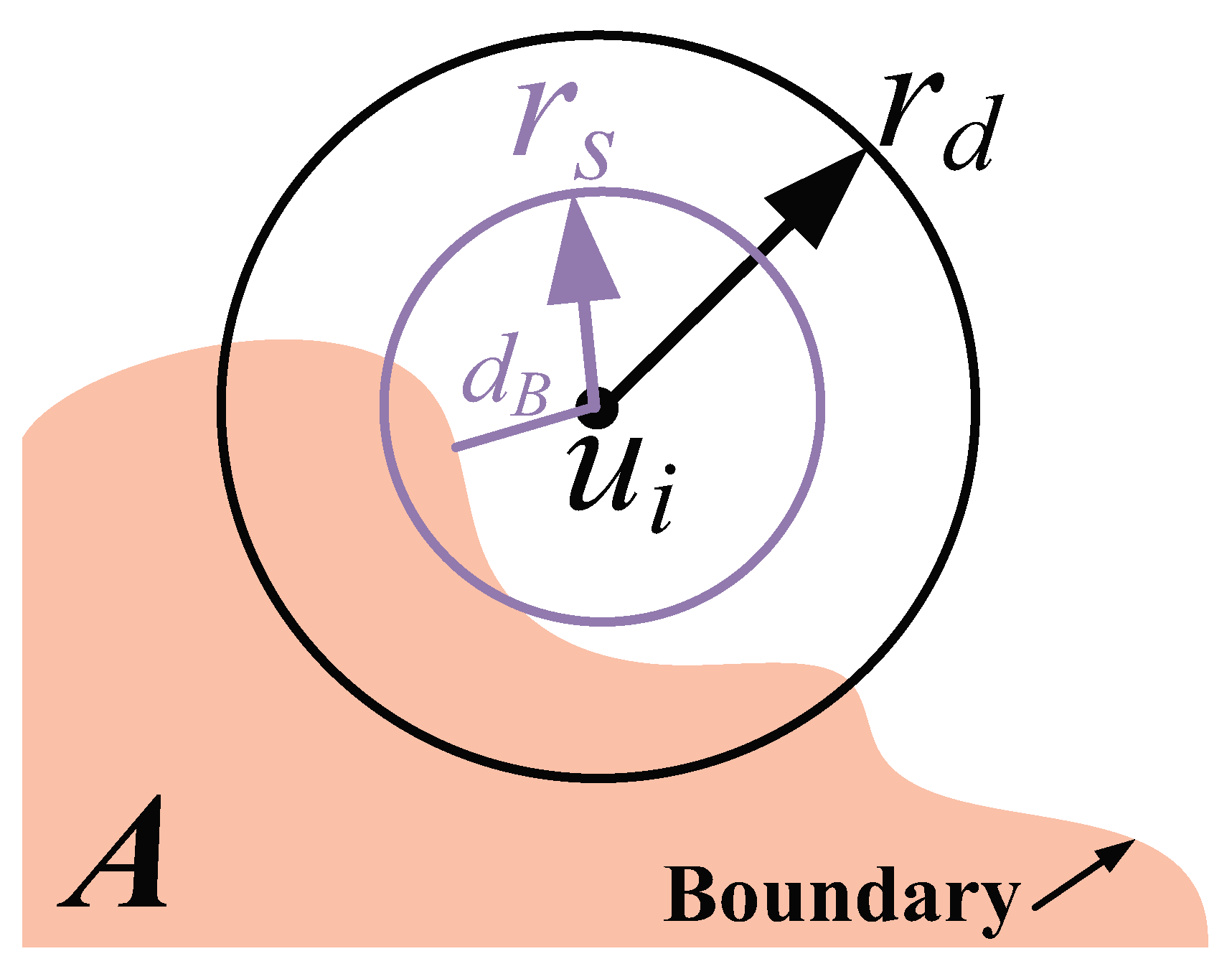
Figure 2.
Coverage map of strong k-barrier coverage around area A, where k=2.
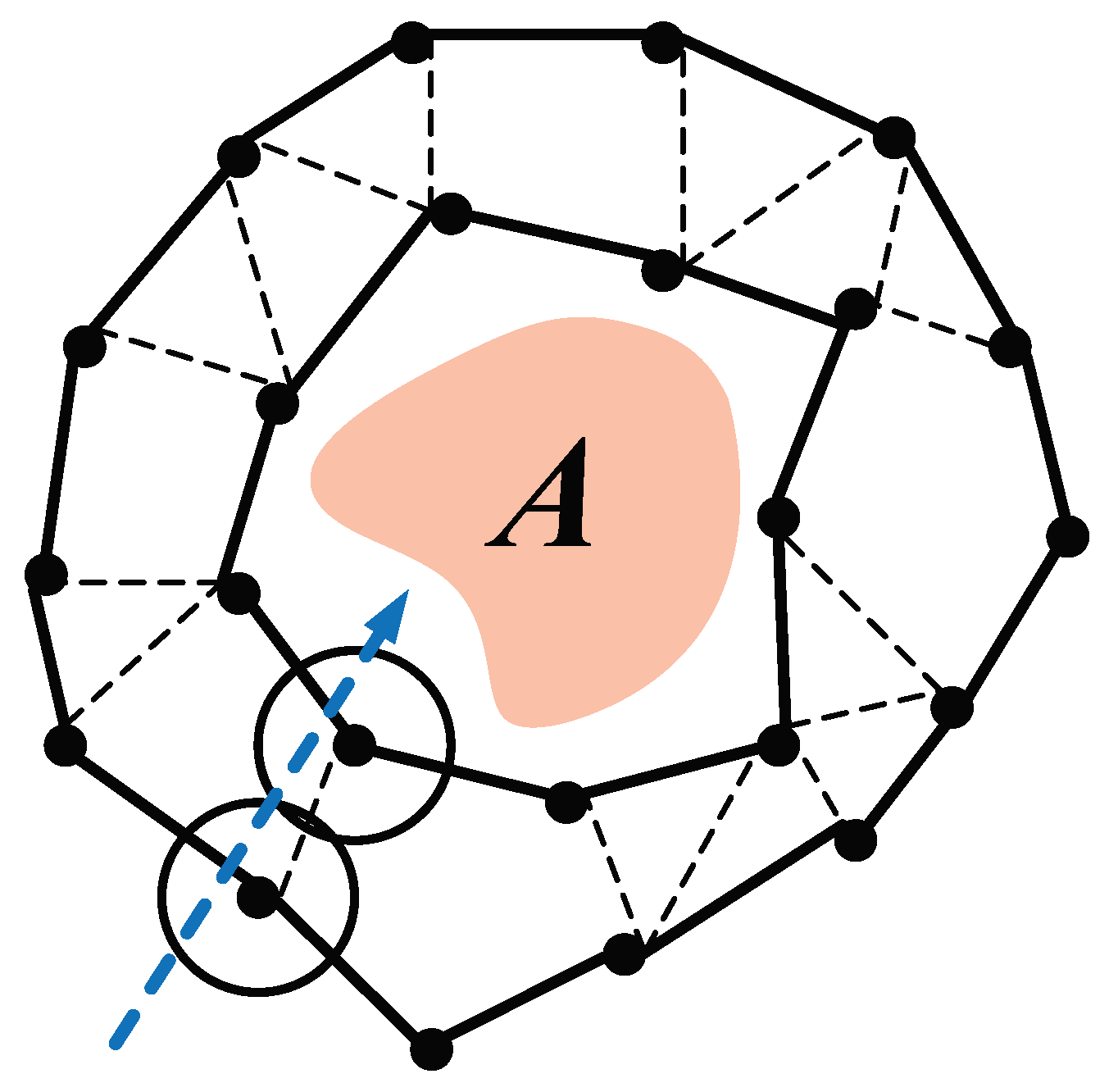
Figure 3.
(a) 2-barrier coverage with multi-level type for a part of region with straight boundary. (b) 2-barrier coverage with line type for a part of region with straight boundary. (c) 2-barrier coverage with multi-level type for a part of region with arc boundary. (d) 2-barrier coverage with line type for a part of region with arc boundary.
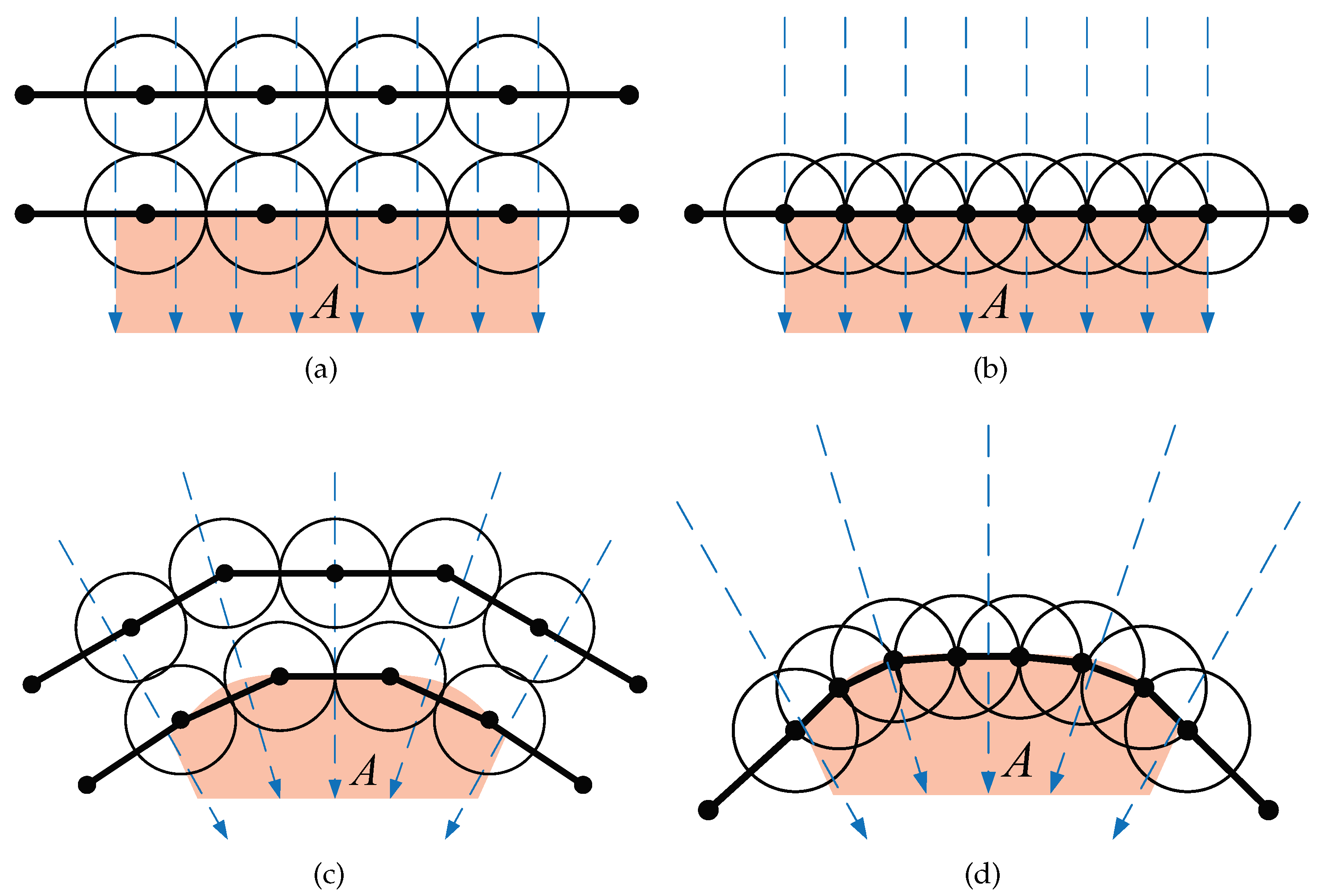
Figure 4.
The paths for boundary seeking: (a) Nodes outside the region move along the boundary in a spiral pattern. (b) Nodes on the boundary remain on the boundary. (c) Nodes inside the region move directly towards the boundary.
Figure 4.
The paths for boundary seeking: (a) Nodes outside the region move along the boundary in a spiral pattern. (b) Nodes on the boundary remain on the boundary. (c) Nodes inside the region move directly towards the boundary.
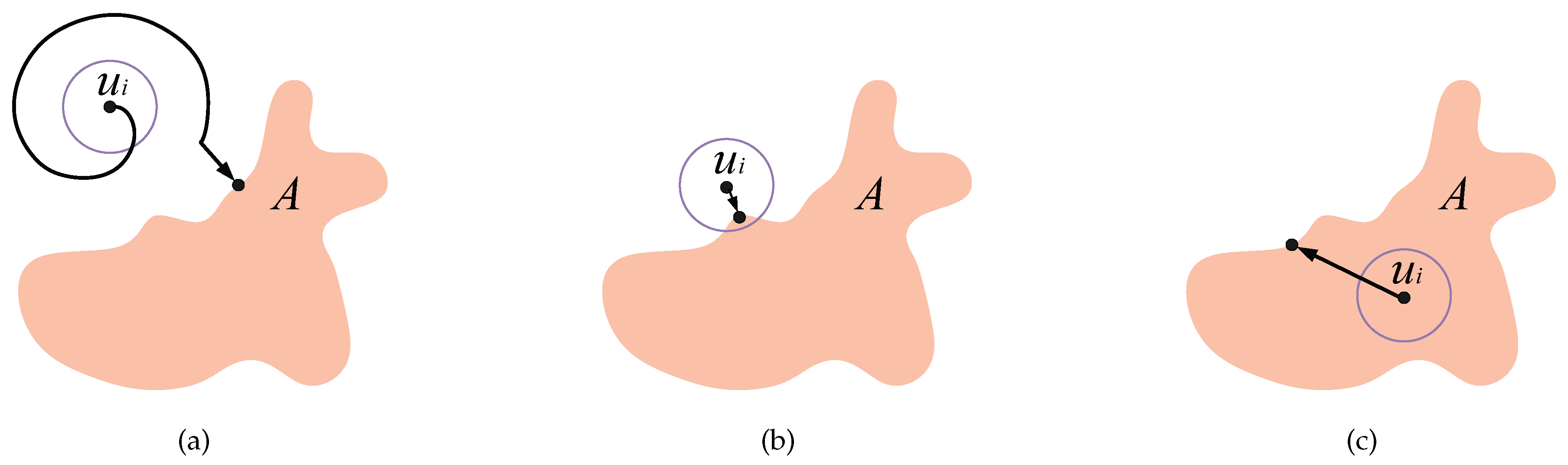
Figure 5.
The movement strategy of the nodes for barrier forming: (a) If a node has no immediate neighbor, it selects clockwise direction and moves along the boundary until meeting the other node. (b) If a node has only one immediate neighbor, it moves away from that neighbor by a distance of along the boundary. (c) If a node has two immediate neighbors and an internal angle , it relocates on the boundary such that . (d) When a node has two immediate neighbors and an internal angle , it positions itself at the midpoint between and .
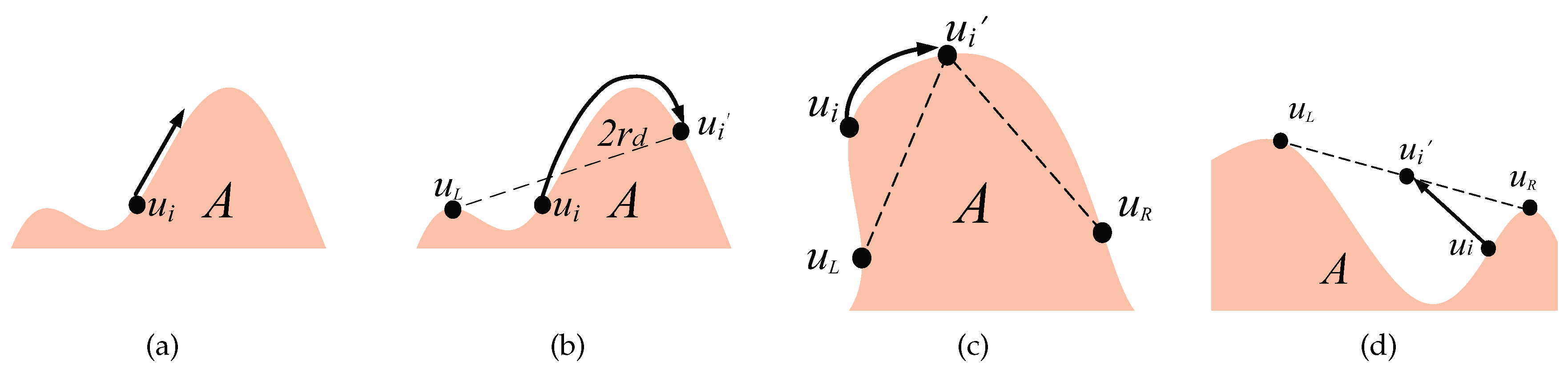
Figure 6.
The Archimedean spiral with pitch .
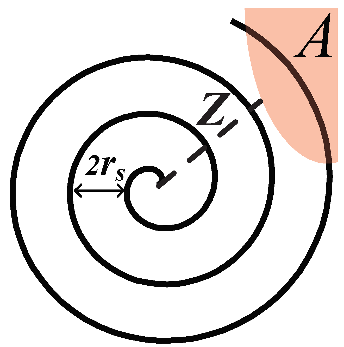
Figure 7.
Four snapshots formed by AutoBar algorithm’s automatic barrier coverage when the initial positions of sensor nodes are randomly distributed in the region.
Figure 7.
Four snapshots formed by AutoBar algorithm’s automatic barrier coverage when the initial positions of sensor nodes are randomly distributed in the region.
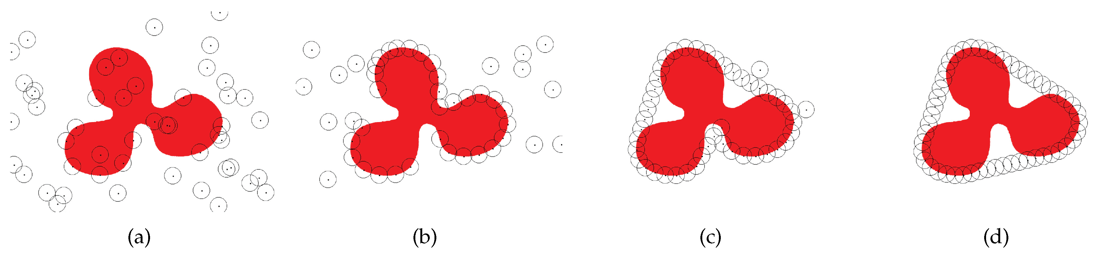
Figure 8.
Four snapshots formed by AutoBar algorithm’s automatic barrier coverage when all sensor nodes are scattered at the same position at the beginning.
Figure 8.
Four snapshots formed by AutoBar algorithm’s automatic barrier coverage when all sensor nodes are scattered at the same position at the beginning.
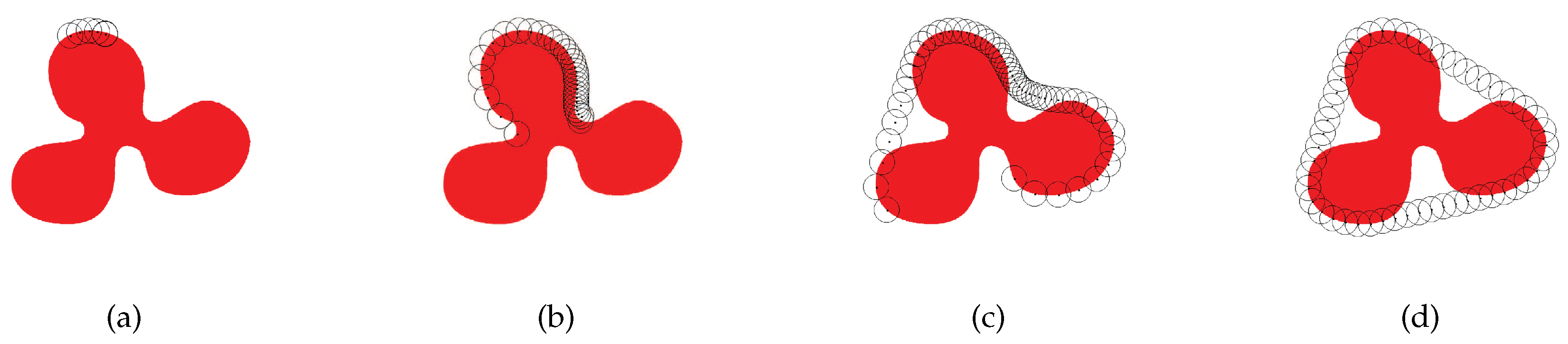
Figure 9.
Comparison between AutoBar and MobiBar on the performance of k when varying n.
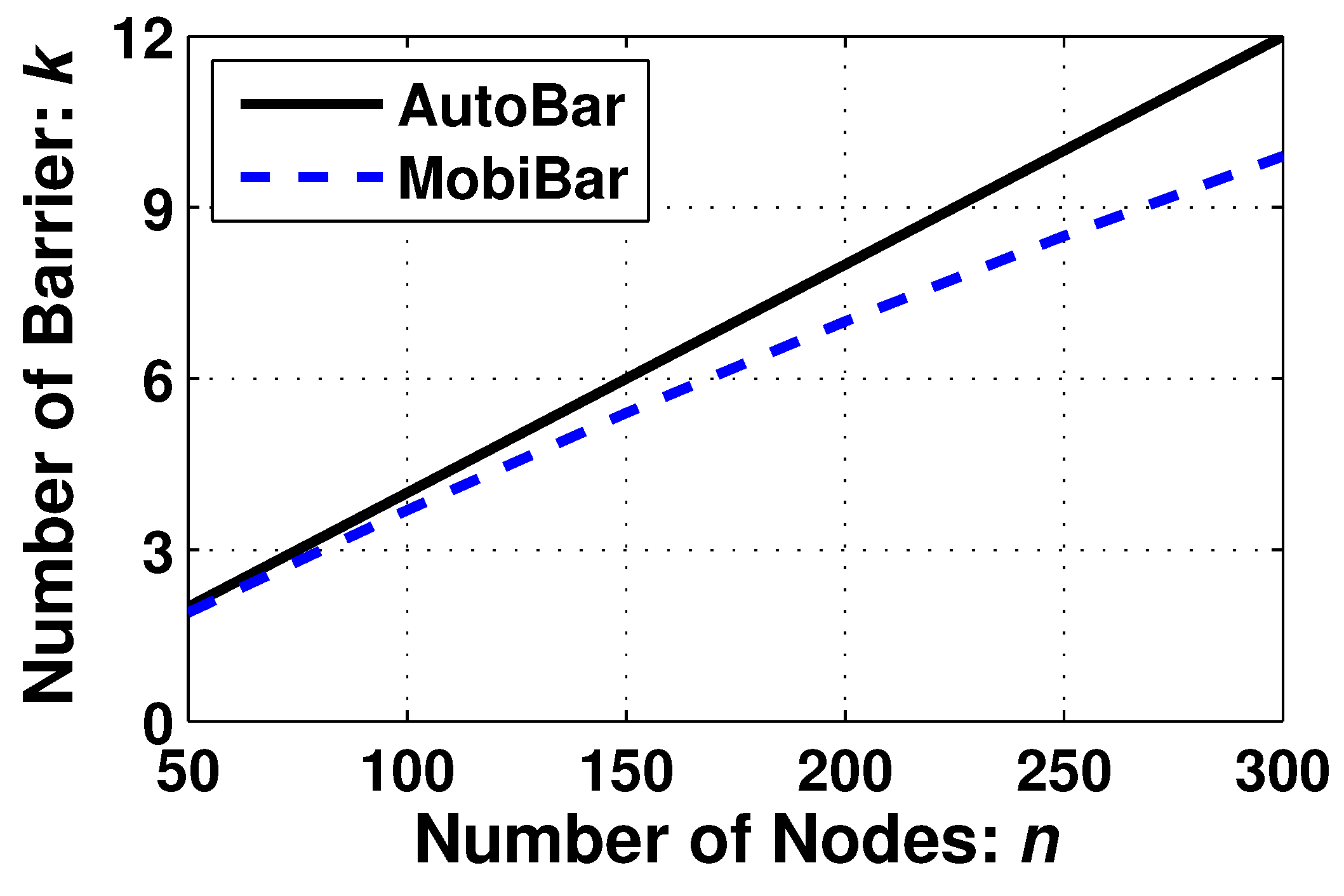
Figure 10.
The formation duration of AutoBar in different deployment types when varying n.
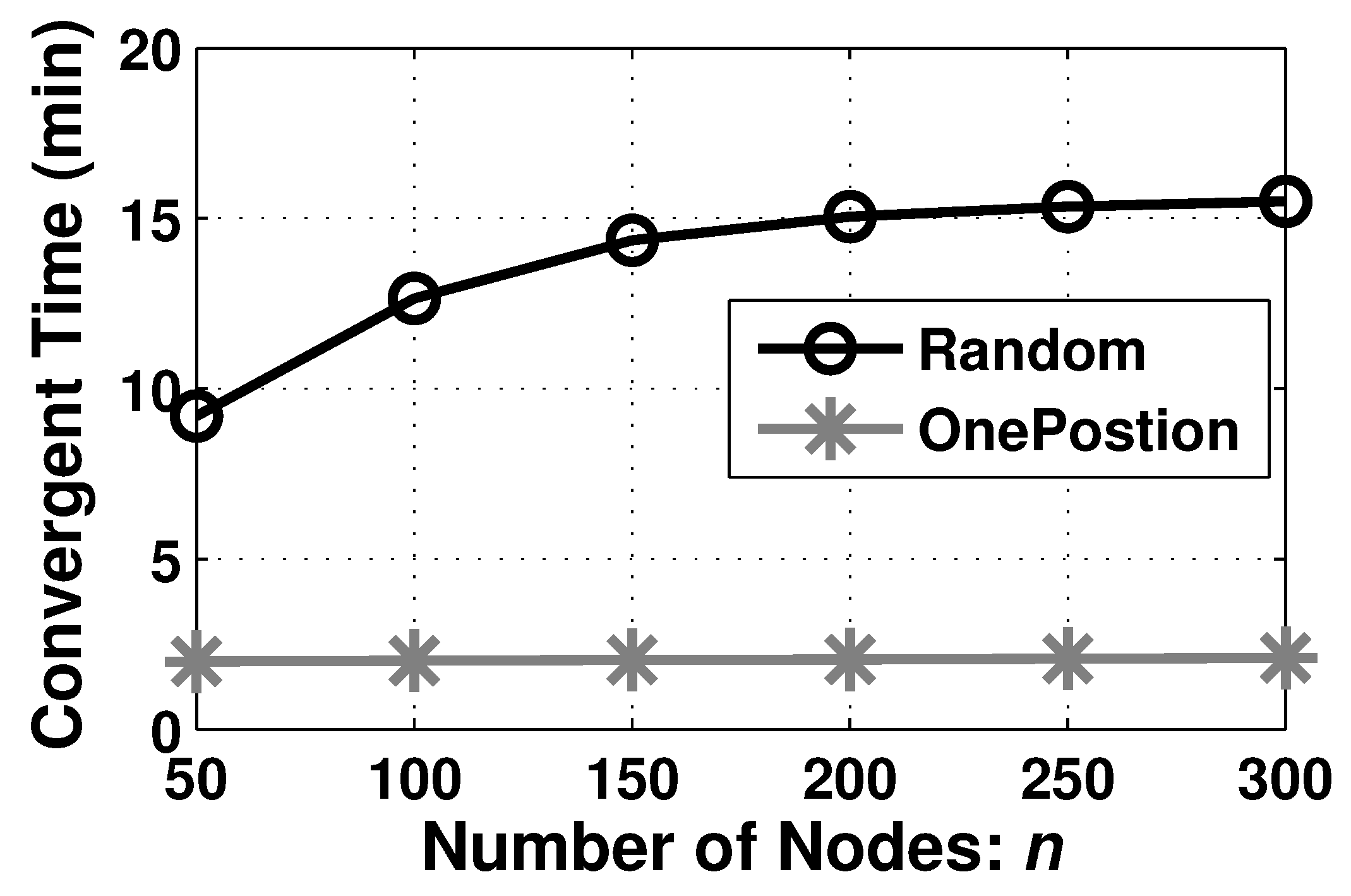
Figure 11.
The communication overhead of AutoBar in different deployment types when varying n.
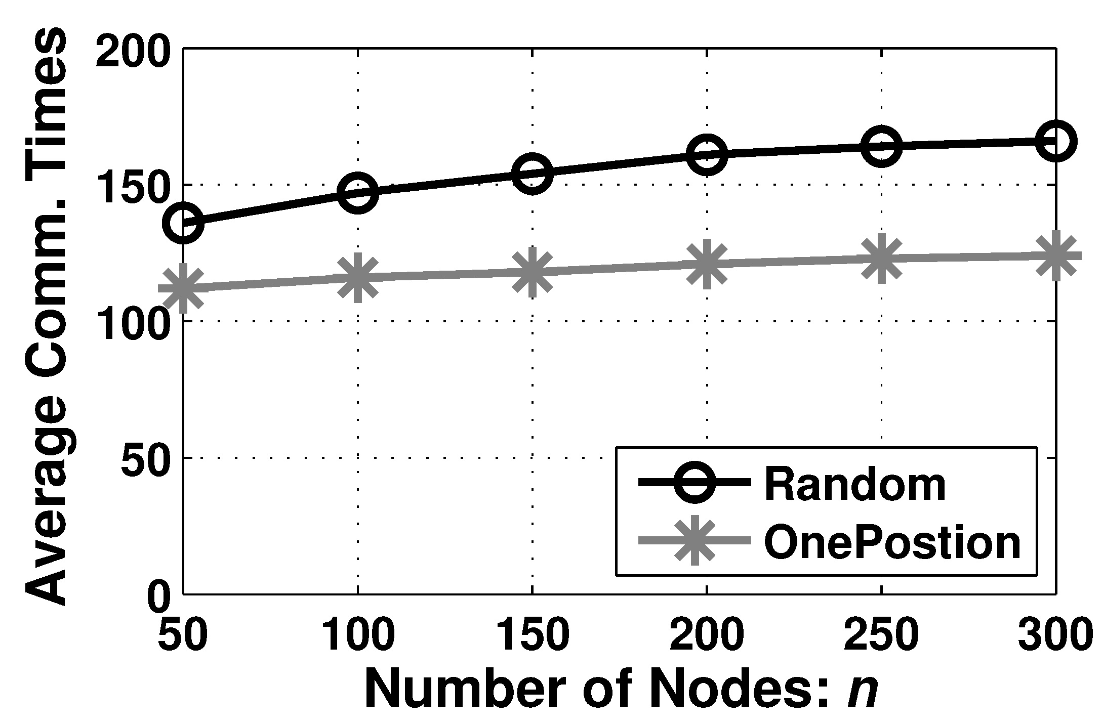

Table 1.
Comparison between classic barrier coverage and warning barrier coverage.
| Barrier Coverage | Classic | Warning |
|---|---|---|
| Target Region | Known | Unknown boundary |
| Sensing Capability | Intruder detection | Visitor detection and |
| boundary detection | ||
| Moving Capability | Mobile/static node | Mobile node |
| Typical Application | Border surveillance | Danger, keep out! |
Table 2.
AutoBar Algorithm.
| AutoBar Algorithm (Executed on node ) |
|---|
| 1: while do |
| // step 1 |
| 2: Sense within area and self-determine; |
| 3: switch (Location) |
| 4: case outside boundary: do |
| 5: spiral_moving(); |
| 6: break; |
| 7: case on boundary: do |
| 8: direct_moving(); |
| 9: break; |
| 10: case inside boundary: do |
| 11: straight_moving(); |
| 12: break; |
| // step 2 |
| // is the next position to move, α is the inner angle |
| 13: Detect the direct neighbors and ; |
| 14: Exchange position information with and ; |
| 15: switch(Num of immediate neighbors) |
| 16: ¡¡¡¡case 0: do |
| 17: ←{clockwise direction with v}; |
| 18: ¡¡¡¡¡¡break; |
| 19: ¡¡¡¡case 1: do |
| 20: ←=&=; |
| 21: ¡¡¡¡¡¡break; |
| 22: ¡¡¡¡case 2: |
| 23: if() do |
| 24: ← the middle position of &; |
| 25: ¡¡¡¡¡¡else do |
| 26: ←=&=; |
| 27: ¡¡¡¡¡¡break; |
| 28: Move to ; |
| 29:end while |
Table 3.
Moving Distance (meters) in Different Deployment Types.
| Num. of Nodes n | 50 | 100 | 150 | 200 | 250 | 300 | |
|---|---|---|---|---|---|---|---|
| Random | Max | 6057 | 7524 | 8463 | 8971 | 9009 | 9054 |
| Ave | 774 | 851 | 910 | 946 | 963 | 972 | |
| Min | 17 | 13 | 10 | 8 | 6 | 6 | |
| OnePosition | Max | 734 | 731 | 728 | 725 | 723 | 720 |
| Ave | 351 | 349 | 348 | 346 | 345 | 344 | |
| Min | 0 | 0 | 0 | 0 | 0 | 0 | |
Disclaimer/Publisher’s Note: The statements, opinions and data contained in all publications are solely those of the individual author(s) and contributor(s) and not of MDPI and/or the editor(s). MDPI and/or the editor(s) disclaim responsibility for any injury to people or property resulting from any ideas, methods, instructions or products referred to in the content. |
© 2023 by the authors. Licensee MDPI, Basel, Switzerland. This article is an open access article distributed under the terms and conditions of the Creative Commons Attribution (CC BY) license (http://creativecommons.org/licenses/by/4.0/).
Copyright: This open access article is published under a Creative Commons CC BY 4.0 license, which permit the free download, distribution, and reuse, provided that the author and preprint are cited in any reuse.


