
Submitted:
06 November 2024
Posted:
06 November 2024
You are already at the latest version
Abstract
Over the past twenty years, camera networks, where individual cameras can function both independently and together, have become increasingly popular. Various application fields may impose distinct requirements on camera networks. In response to these demands, several coverage models have been developed in the scientific literature, such as area, trap, barrier, and target coverage. In this paper, a new type of coverage task, the Maximum Target Coverage with k-Barrier Coverage (MTCBC-k) problem is defined. Here, the goal is to cover as many moving targets as possible from time step to time step, while continuously maintaining k-barrier coverage over the region of interest (ROI). This approach is different from independently solving the two tasks and then merging the results. Generally, multiple camera configurations can ensure k-barrier coverage. The challenge is to find, at each time step, the optimal configuration where the cameras providing barrier coverage can also assist in covering targets, while the rest of the cameras efficiently cover the remaining targets. An ILP formulation for the MTCBC-k problem is presented. Additionally, two types of camera clustering methods have been developed. This approach allows for solving smaller ILPs within clusters, and combining their solutions. Furthermore, a polynomial-time greedy algorithm has been introduced as an alternative to solve the MTCBC-k problem. The conducted simulations convincingly supported the usefulness of both the clustering and the greedy methods.
Keywords:
barrier coverage
; target coverage
; directional sensors
1. Introduction
In the last two decades, camera networks, where the separate cameras can operate autonomously and collaboratively, have become increasingly popular. For instance, such networks are used to monitor and manage traffic flow in urban areas, helping to reduce congestion and improve road safety. Farmers employ them to monitor crop health, detect pests, and manage irrigation systems more efficiently. They are also integral to smart city initiatives, providing data for public safety, environmental monitoring, and efficient resource management. Additionally, intruder detection is one of the most important applications of these systems, aiming to detect any trespasser attempting to penetrate areas of interest (ROI) such as national borders or critical infrastructure.
The different application fields may pose different requirements on camera networks. In certain situations, it is important to keep an eye on every point of the monitored area by one or more sensors. This is referred to as full area coverage in the related scientific literature [1]. However, achieving this may require significant resources, and in many cases, it is sufficient for the system to meet less strict conditions. For example, a network with trap coverage ensures that any moving object can travel only a limited (known) distance before it is detected by a camera. In other words, at any given moment, one can either accurately determine the exact location of a moving object or identify a coverage hole with a known diameter where it is confined [2]. Another variant of the coverage problem is the k-barrier coverage. Here, the network must be deployed in such a way that any intruder or moving object crossing the ROI will inevitably pass through the field of view of k different cameras [3]. Possibly the simplest version of the coverage related problems is target coverage, where the objective is the continuous observation of static or moving objects [1]. In some cases, the targets may have different priorities [4].
In this paper, networks composed of Pan-Tilt-Zoom (PTZ) cameras are examined. In short, such cameras are equipped with motorized mechanisms that allow them to rotate horizontally and vertically, and zoom in or out. The cameras are modeled as directional sensors, meaning their sensing region is represented as a sector of a circle, unlike the isotropic sensor model, which represents the sensing region as an entire circle. In practice, a PTZ camera is capable of sweeping all the sensing orientations continuously, however, the simplifying assumption is often made in scientific works that a camera can only take on a finite set of sensing directions [5]. This is also the case in this paper. The goal is to solve a combination of the barrier and target coverage tasks. This combination is inspired by the dilemma of wanting to simultaneously track the paths of already detected moving objects while not missing newly arriving ones. At national borders, a possible strategy for intruders is for one group to intentionally distract the cameras, allowing another group to slip through the temporarily unmonitored corridor unnoticed. An effective solution to the combined barrier-target coverage problem would, in addition to its other obvious advantages, also provide protection against such strategies.
Further clarifying the task to be solved, it is assumed that the barrier to be monitored is an open belt, i.e, it can be represented as an elongated rectangle [3]. The positions of the cameras are supposed to be given. The deployment can be random as well as the result of applying a certain strategy. Camera networks often function as part of larger, heterogeneous sensor networks [6]. As a result, in addition to the cameras the positions of moving objects are determined step-by-step with the help of other sensors. From the perspective of the task being examined, this is the ideal scenario. However, the simulations also modeled the case where cameras do not receive any additional information about the objects to be observed beyond their own detections. In the scientific literature, two types of barrier coverage are considered: strong and weak [7]. The focus here is on the strong type. In this case, regardless of how a moving object crosses the ROI, it cannot avoid detection. A brief description of weak barrier coverage is included in the Related Works section (Section 2).
When tracking a moving object, at every moment, essentially a target coverage task needs to be solved, i.e., the number of covered targets should be maximized. Meanwhile, for a predetermined k, k-barrier coverage must also be continuously maintained. This setup differs from solving the two tasks separately and somehow merging the results. Generally, more than one camera configuration may exist that ensures k-barrier coverage. The challenge is to find, at each time step, the optimal configuration where, on one hand, the cameras providing barrier coverage can simultaneously assist in covering targets, and on the other hand, the remaining cameras cover the remaining targets as efficiently as possible.
The contributions of this paper are as follows.
- (i)
- A new type of coverage problem, the Maximum Target Coverage with k-Barrier Coverage (MTCBC-k) problem is defined. The corresponding ILP is also formulated. To the best of our knowledge, we are the first to examine this question.
- (ii)
- A new ILP formulation for the maximum coverage problem has been provided, which is significantly different from the ones given in [8,9,10]. This formulation can be easily integrated with the part of the ILP of the MTCBC-k problem responsible for ensuring k-barrier coverage. Additionally: (a) the resulting ILP also allows for certain optimizations regarding the cameras. Examples of these optimizations include the number of cameras and the cost of their usage. (b) Furthermore, the relative importance of the targets can also be specified using the cost associated with them. (c) Finally, an upper limit can be set for the number of cameras that can be used for solving the task.
- (iii)
- While the ILP formulation offers an optimal solution for the MTCBC-k problem, it does not scale well for large problem instances. To mitigate this difficulty, two types of camera clustering methods have been developed. This allows for solving smaller ILPs within clusters, and by combining their solutions, a solution to the original MTCBC-k task can be obtained. In addition, a polynomial-time greedy algorithm has also been introduced. This method guarantees only 1-barrier coverage alongside target coverage, but in practice, this value is often higher and closer to k. The conducted simulations convincingly supported the usefulness of both the clustering and the greedy methods.
The rest of the paper is organized as follows. The related literature is presented in Section 2. In Section 3 the directional sensor model and the maximum flow problem are explained. The latter is used in the ILP formulation of the MTCBC-k problem. In Section 4 the MTC and MTCBC-k problems are defined. The corresponding ILP formulations are given in Section 5. The clustering and the greedy algorithms are explained in Section 6. In Section 7 the experiments are presented. Finally, in Section 8 the conclusions are drawn.
2. Related Work
One of the seminal papers that examined the question of target coverage for directional sensor networks is [8]. In this paper, the Maximum Target Coverage with Minimum Sensors (MCMS) problem was defined and shown to be NP-complete. The authors provided an ILP formulation of the task and developed centralized and greedy algorithms offering approximate solutions.
In [9], it has been proven that the Maximum Target Coverage (MTC) problem is already NP-complete in the case of directional sensors without requiring the minimality of the number of the involved sensors. This is the version of the task that is addressed in this paper. It was referred to as the directional cover set (DCS) problem in [9]. As a matter of fact, the focus of the authors of [9] was not on this question, but on an extended variant of it – the multiple directional cover sets (MDCS) problem, where they aimed to identify several possible coverings in order to be able to switch between them and thus extend the lifetime of the network.
The idea of forming clusters of sensors to more effectively solve the MCMS problem was introduced in [10]. The authors also presented a different ILP formulation of the task and offered a slightly improved centralized greedy algorithm. The greedy algorithm described in this paper builds upon this latter version.
In [11], a more complex form of the clustering task was examined, where the sensors within a cluster could communicate with each other as well as sensors from different clusters. To represent message sending and receiving, the directed communication model was used, where only those neighboring sensors that lie within a specified sector could receive a message of a sensor. At first glance, it may seem that the question examined in our paper is similar to the one addressed in [11]. To ensure that each message reaches every sector, a chain needed to be formed from the communication sectors where every sector falls within a communication sector of at least one other sector. This might appear similar to the 1-barrier coverage task, where a chain of the detection sectors of the sensors must be created that runs through the observed area. In addition to forming these sector chains, the maximum target coverage problem needs to be solved in both cases. In reality, however, there are several important differences between the two tasks. The most significant of these is that the communication sectors are independent of the detection sectors, thus having no impact on how the maximum target coverage problem is solved. Whereas in the combined solution of barrier and target coverage tasks, a detection sector that plays a role in barrier coverage can also be crucial for target coverage. In other words, if the positions of the targets change, it has no effect on the chain formed by the communication sectors, while the chain providing barrier coverage can significantly transform.
[4] is one of the earliest paper where targets were distinguished based on their importance. A higher-priority target must be monitored by multiple sensors. However, the efficiency of detection is also influenced by the distance between the target and the sensors. For example, it may be sufficient to use two sensors for a nearby target, but if the sensors are distant, three might be needed. The just described priority-based target coverage problem has gained popularity and further been examined in subsequent papers like [12]. The type of prioritization among targets enabled by the ILP formulated in our paper is different and less sophisticated compared to that introduced in [4].
Regarding the question examined, a somewhat related work to ours is [13]. Here, the goal was to cover as many moving targets as possible at each time step, and reinforcement learning was utilized to learn the optimal strategy. The effectiveness of the resulting solution was compared, among other methods, with the algorithm solving the appropriate instance of the MCMS problem at each time step.
In the context of sensor networks, the barrier coverage problem was introduced in [3]. The authors based their work on the isotropic sensor model, however, many of their results also remain valid for the directional sensor model. They distinguished weak barrier coverage from strong barrier coverage. In the latter case, regardless of how a moving object crosses the ROI, it cannot avoid detection. While in the former case, there is a given path through the ROI, and detection is only guaranteed if the object chooses a path that is congruent with this path. Two paths are congruent if one can be transformed into the other through translation and orientation.
In [14], an ILP was presented that for given static directional sensors determines the level of barrier coverage that the network can provide. This ILP is very similar to the part of the ILP solving the MTCBC-k problem which ensures k-barrier coverage. It is also based on the maximum flow problem over a network graph created from the coverage graph of the sectors of the sensor network. The authors also developed polynomial-time approximating solutions to the k-barrier coverage problem. In the greedy algorithm offering an approximate solution to the MTCBC-k problem, a subroutine with the same purpose was also introduced, but this method differs from those mentioned earlier.
In [15], the same question was addressed as in [14], however, here it was assumed that the directional sensor can sweep all the directions along its circle, whereas in the previous work the number of available directions was finite, just as it is in our work. The authors developed a polynomial algorithm to determine whether the given sensor network can provide 1-barrier coverage. An energy-efficient solution was also presented that approximately minimized (1) the total and (2) the maximum rotation angles while rotating the cameras to ensure barrier coverage.
Finally, in [16] a new type of coverage problem called the target-barrier coverage problem was defined. Although the name of the problem includes both the terms barrier and target, it addresses a question entirely different from the one examined in our paper. Specifically, a target-barrier is a continuous circular barrier formed around the target. It has a parameter that defines the minimum distance of the constructed barrier from the target. The authors focused on how to minimize the number of members required to construct target-barriers in a distributed manner while satisfying the constraint and minimizing the amount of message exchange required. The target-barrier coverage problem is still an actively researched question. One of the most recent papers written on the topic is [17].
In summary, the MTCBC-k problem introduced in this paper differs from all the presented works. While it draws ideas from them, it addresses a new type of coverage problem that, to the best of our knowledge, has not been researched before.
3. Preliminaries
In order to work in a formal context with PTZ cameras, an appropriate model needs to be introduced. This is accomplished in Section 3.1. There and in what follows, PTZ cameras will be referred to as sensors.
To ensure k-barrier coverage, a special instance of the maximum flow problem needs to be solved. To be able to refer to the relevant concepts precisely, the definition of the problem is included in Section 3.2.
3.1. Directional Sensor Model
Unlike isotropic sensors, a directional sensor generally has an angle of view less than 360 degrees, so it cannot sense the entire circular area around itself. In a two-dimensional plane its sensing region can be viewed as a sector. Such a sector of sensor S can be characterized by a quadruple . Here, p is the location of S given in Cartesian coordinates , while o and denote the orientation and angle of view of S respectively. Finally, d specifies the maximum detection distance. See Figure 1 (a) for further details.
To be able to solve the coverage and tracking problems effectively, it is assumed that a directional sensor can only take a finite set of orientations. To simplify the notation and facilitate further explanations, it is supposed that all sectors have the same angle of view and maximum detection distance, and the orientations divide the 360 degrees into equal parts. However, this is not necessary, as the algorithms to be presented work the same way even when these assumptions do not hold. For instance, during the simulations, triangles were used to represent sectors, and the individual sectors could overlap with each other (Figure 1 (b)).
To determine when sensor S detects a target, the Target in Sector (TIS) test is used [1]. Informally, this test requires that the target must fall within the detection range of S, and it must also lie within the field of view of S based on its current orientation. In other words, this means that in the two-dimensional plane the position of the target must be inside or on the edge of the currently active sector of S. Formally:
Here is the vector pointing from the location of S to the target, denotes the length of in the Euclidean space, is the unit vector with the same direction as the orientation of S, while d and stand for the maximum detection range and angle of view as before.
Definition 1.
For a given sensor S, sector of S and target t, coverst, if Equation 1 holds for and t. S covers t, if at least one of its sectors covers t.
3.2. Maximum Flow Problem
Let be a network with two distinguished vertices being the source and the sink, respectively. Denote by the capacity function that determines the maximum amount of flow that can pass through an edge. A flow is a map that satisfies two properties.
- Capacity constraints:
- Conservation of flows: . In other words, the sum of the flows entering a vertex must equal the sum of the flows exiting the same vertex, except for the source and the sink.
The value of a flow is defined to be the sum of the flows given on the edges originating from the source, . The task is to find the flow with the maximum value.
4. Problem Statement
4.1. The MTC Problem
Let be the set of sensors. Denote by the sectors belonging to . Obviously, a sensor cannot look in two directions at the same time. The next definition formalizes this phenomenon.
Definition 2.
With the above notations, is apermissible sector selection, if there are no two sectors in that belong to the same sensor.
Let be the set of targets. Denote the subset of those targets that are covered by sector .
Definition 3.
With the above notations, in the Maximum Target Coverage (MTC) problem, one must find the permissible sector selection coverage for which the cardinality of is maximal. In other words, the permissible sector selection covering the maximum number of targets is to be found.
4.2. The MTCBC-k Problem
First, the barrier coverage problem is defined. Here, an elongated rectangle, referred to as open belt [3], is considered where the horizontal sides are substantially longer than the vertical ones. A crossing path is defined as a path that traverses the belt from one horizontal side to the other. The idea is to place the sensors and select the active sectors in such a way that, no matter which way an object moves, it cannot avoid being detected when crossing this belt. Informally, in case of k-barrier coverage, it is guaranteed that this object is detected by k different sensors.
Let be the sensors deployed on an open belt and let be a permissible sector selection. Denote by the set of targets, including both static and moving objects.
Definition 4.
With this notation, a path l crossing the open belt is said to bek-covered (by ), if for k different sectors in , , . The open belt isk-barrier covered (by ), if all crossing paths are k-covered (by ) [3].
Definition 5.
In the Maximum Target Coverage with k-Barrier Coverage (MTCBC-k) problem, one must find the permissible sector selection coverage that provides k-barrier coverage on the open belt. In addition, among the permissible sector selections that guarantee k-barrier coverage, must be the one covering the maximum number of targets.
To be able to solve the MTCBC-k problem, it is worthwhile to understand the graph-based characterization of k-barrier coverage. For a given open belt, deployed sensors, and permissible sector selection , a coverage graph can be defined. The vertices of represent the sectors, plus two extra vertices, s and t, stand for the left and right boundaries of the belt respectively. Two sector vertices are connected with an undirected edge if their intersection is not empty. s (or t) is connected with a sector vertex if the sector intersects the left (or the right) boundary. An example can be found in Figure 2. Exactly the same way as in [3], the following theorem can be proven.
Theorem 1.
An open belt with a sensor network is k-barrier covered by permissible sector selection if and only if there exist k vertex-disjoint paths from s to t in .
5. ILP Formulations
5.1. The MTC Problem
In this section the ILP, , is formulated that solves the MTC problem. When tracking moving objects, should be updated and computed at each time step.
As before, let be the sensor network deployed on the open belt. Let be the set of targets. In addition to the actual sectors of the sensors, to each target a dummy sector is assigned. This sector covers only the given target and does not belong to any sensor (Alternatively, it can also be said that each dummy sector belongs to a new sensor that only has this sector, or the rest of its sectors do not cover any targets.). The role of the dummy sectors will become apparent soon. If denotes the number of the real sectors, then the total number of sectors is , where m is the number of targets.
The elements of the variable vector of will represent whether a sector is selected to be active or not, hence they can take 0 or 1 values. It is assumed that the last m elements of correspond to the dummy sectors.
The cost vector, , is defined as follows:
In other words, the element of is 0 if it represents a real sector, and 1 otherwise. The aim is to minimize , where is the dot product of and . Obviously, is minimized if as few dummy sectors as possible are used to cover the targets.
As constraints of , two requirements need to be expressed. Firstly, it needs to be guaranteed that each solution encodes a permissible sector selection. Secondly, this permissible sector selection must cover all targets. Note that dummy sectors were introduced specifically to ensure the existence of such permissible sector selections. Since, clearly, a permissible sector selection containing all dummy sectors always covers all targets.
Formally, is:
Here,
Basically, the elements together form the incidence matrix of the sensors and their sectors. Note that if the element of , , represents a dummy sector then is 0 for all sectors, i.e., for all i.
On the other hand,
The elements together constitute the incidence matrix between the targets and the sectors.
It is easy to see that if Inequality 2 is satisfied then encodes a permissible sector selection. Meanwhile, Inequality guarantees that each target is covered by at least one sector. Furthermore, the minimality condition ensures that among the permissible selections that provide a complete coverage, the ILP solutions will be those where the number of dummy sector used is minimal, or to put it differently, the number of targets covered by real sectors is maximal. All together this shows that a solution of encodes a solution to the MTC problem.
Further considerations.
Optionally, the number of usable sensors can also be limited. Simply add inequality
to the constraints of . Here,
Evidently, if is a solution to this extended version of then in the encoded permissible sector selection at most r sectors, and consequently r sensors, are used.
Note also that the first elements of are 0, which means additional costs can be introduced for the real sectors. For example, if all these elements are set to 1 and the cost of using a dummy sector is higher than the number of the real sectors, then a solution to this modified ILP also minimizes the number of employed sensors. Alternatively, the sum of the angles of rotation required to move from one sector selection to another can be minimized as well.
Lastly, the targets can also be distinguished from each other. For example, if target t must be covered and there is a real sector capable of covering it, then the dummy sector corresponding to t should not be added to . This ensures that t is covered by a real sector in any solution.
The targets can also be distinguished from each other based on the costs assigned to their associated dummy sectors. Suppose that the set of targets contains both static and moving targets. Then, for example, if , where and denote the costs of the dummy sectors of static and moving targets respectively, then covering 4 moving targets is equally important as covering 1 static target.
5.2. The MTCBC-k Problem
In the ILP, , that solves the MTCBC-k problem in addition to covering the maximum number of targets, k-barrier coverage must also be ensured. Recall that by Theorem 1, an open belt is k-barrier covered by a permissible sector selection if and only if there are k vertex-disjoint paths from s to t in the coverage graph representing , . In what follows, a network graph with the appropriate capacities will be constructed in such a way that the size of the maximum flow will be equal to the maximum number of these vertex-disjoint paths (When Menger’s theorem is proven by reducing it to the Max-flow min-cut theorem, it is shown that for any undirected graph with selected vertices s and t, a network can be created where the value of the maximum flow is equal to the number of vertex-disjoint paths between s and t[18]. Here, basically, the same construction is utilized.). The maximum flow problem can be formulated as a linear program, and this construction will be used in to guarantee k-barrier coverage.
Let be an open belt with deployed sensor network . Denote by the set of targets. In the construction of the aforementioned network graph, first a coverage graph, , is created. This will be very similar to the coverage graph of a permissible sector selection. The only difference is that, in this case, not just a single permissible sector selection will be represented, but all of them. Next, will be modified in two steps. First, since capacities and flows can be defined on edges and represents sectors as vertices, these vertices will be replaced with edges. Then, the undirected edges will be converted into directed ones.
Considering the details, as in the case of a coverage graph belonging to a permissible sector selection, the vertices of stand for sectors of and the left and right boundaries of the open belt. These last two vertices are denoted by s and t. The edges of s and t can be defined exactly in the same way as before. Two sector vertices are connected if the sectors belong to different sensors and their intersection is not empty.
Next, each sector vertex v of should be substituted by a directed edge . Finally, the remaining undirected edges of are changed to directed ones. Edges with s (or as an endpoint should be converted to edges originating from s (or ending in t). Additionally, each edge between sector vertices should be replaced with two directed edges: and . An example can be found in Figure 3. Finally, the capacity of the edges derived from sector vertices is set to 1, while the capacity of the remaining edges is defined to be infinity. Denote the resulting network as .
Definition 6.
With the above notations, a flow f in ispermissibleif there are no two sectors represented by the sector edges with positive flow that belong to the same sensor. Here, a sector edge is an edge derived from sector vertex u in .
Theorem 2.
With the above notations, there is a permissible sector selection, , in that provides k-barrier coverage on if and only if there exists a permissible flow of value k from s to t in .
Proof.
By Theorem 1, is k-barrier covered by if and only if there are k vertex-disjoint paths from s to t in . From the definition of a permissible sector selection it follows that no two sectors involved in these paths belong to the same sensor. is a subgraph of , hence these paths are also included in . Now, note that if is a path in , where are sector vertices, then is a directed path in , and vice versa. Thus, there exist k different paths from s to t in such that no two sector edges in the paths represent sectors that belong to the same sensor. The capacities of sector and non-sector edges are 1 and ∞ respectively, therefore on each such path a flow of value 1 can go from s to t. Since the number of these paths is k, this proves the existence of a permissible flow of value k from s to t in . By reversing the above reasoning, the other direction of the statement can also be proven. □
Remark 1.
Paths in where no two sectors, represented by the sector edges of these paths, belong to the same sensor, are calledsensor-disjoint. Consider a flow of value k in . In the proof of Theorem 2 it has just been shown that the edges with positive flow form k sensor-disjoint paths from s to t. Obviously, sensor-disjoint paths do not even share a common edge. This is because at least one ending vertex of each edge in represents a sector.
Based on Theorem 2, when formulating , the existence of a permissible flow of value k needs to be ensured. This in turn guarantees the existence of a permissible sector selection providing k-barrier coverage on .
The elements of the variable of stand for sector, non-sector edges of , and dummy sectors as in the case of . Their numbers are and m respectively, where m is the number of targets. It is also assumed that the elements appear in in the aforementioned order. The first elements represent the flow on the sector and non-sector edges of . Since the goal is to encode whether a sector is selected or not, the flow of the sector edges can be either 0 or 1, while the non-sector edges can have arbitrary non-negative flows. It follows from the Ford-Fulkerson method that if the capacities are integer or infinite values, as is the case in , then there exists a maximum flow f such that is an integer for every edge [18]. This statement guarantees that despite restricting the possible values of the "sector elements" in to 0 or 1, a maximum flow can still be found. Finally, the last m elements of represent whether a dummy sector is selected or not for covering the targets, thus they can also have either 0 or 1 values.
The goal formulated with cost optimization is the same as in : to minimize the number of dummy sectors used for covering the targets. Consequently, the cost vector, , is basically the same as :
The constraints of represent the conservation of flows rule, the capacity constraints, and they also ensure the existence of a k-valued flow from s to t in . In addition, a slight modification of Inequalities 2 and should also be included in order to guarantee that a solution can only encode a permissible sector selection which covers all of the targets.
For vertex v of denote by , the sets of ingoing and outgoing edges of v, respectively. Now, can be defined as follows:
where n and m are the numbers of sensors and targets, respectively, and
Thus, Equality guarantees that a flow of value k leaves s in , while Equality 5 and Inequality ensure the arrival of this flow at t.
The definitions of and are very similar to those given in Inequalities 2 and . The only difference is the presence of non-sector edges in this case. However, these have no role here. Thus, and can be defined in the same way as before for sector edges and dummy sectors, and can be set to 0 for non-sector edges.
Based on what has been discussed so far in this section, it is easy to see that a solution to indeed represents a solution to the MTCBC-k problem.
Further considerations.
Note that the number of sensors to be used can be limited in the same way as in the case of . The same can be said about the possible cost assignment to real sectors and the opportunity to distinguish between targets.
5.3. Supplementary ILP Formulations
In what follows, it will be important to find a permissible sector selection that provides k-barrier coverage on . Moreover, among the permissible sector selections that also ensure k-barrier coverage should contain the minimal number of sectors – which entails that it also contains the minimal number of sensors. Next, it is shown how can be transformed into another ILP, , whose solution encodes a permissible sector selection with the desired property.
Targets play no role in the formation of k-barrier coverage. Thus the elements of the variable of , , only represent the sector and non-sector edges of , i.e., the dummy sectors are not included. Inequality also needs to be removed from the constraints. The rest of the constraints of can be preserved without any further change. Note that in all of these constraints in the positions of the dummy sectors only 0s appeared, consequently, the deletion of these columns does not result in any significant changes.
The cost vector, should be defined as follows:
needs to be minimized.
With this, is fully defined. It is easy to see that a solution of encodes a permissible sector selection that provides k-barrier coverage over . Moreover, the minimization in the objective guarantees that the number of involved sectors is minimal.
Maximum level of barrier coverage.
To decide how strict barrier coverage one wishes to ensure, one must know the maximum level of barrier coverage that the sensor network is capable of providing. can easily be transformed into another ILP, , that answers this question.
The structure of the variable of is the same as that in . From the set of constraints in , Equality , which guarantees the existence of a flow of value k leaving s, should be removed. The rest of the constraints can remain unchanged. As an objective, one should require that the value of the flow leaving s be maximal. Thus, should be defined in the same way as the coefficients of Equality
needs to be minimized.
Clearly, if is a solution of , then the value of is equal to the maximum level of barrier coverage that can provide over . Note that was already formulated in [14]. Here, it was only reiterated for sake of completeness.
6. Approximations of the MTCBC-k Problem
Although the ILP formulation provides an optimal solution for the MTCBC-k problem, it does not scale well for larger instances. To handle this problem, two approaches are proposed. In the first case, clusters are formed from the sensors, where the ILP becomes solvable due to the smaller size. The solutions obtained for the clusters are then combined to provide a solution to the original MTCBC-k problem. In the second case, a polynomial-time greedy algorithm, , is developed. This guarantees only 1-barrier coverage instead of k. However, the simulations have shown that in practice, the level of the provided barrier coverage is rather close to k.
6.1. Clustering
The clusters can be created both horizontally and vertically. See Figure 4 (a,b) for examples. In the horizontal case, the main idea is to create k clusters in such a way that the selected sectors within each cluster provide at least 1-barrier coverage on the open belt. This way, the appropriate instance of the MTCBC-1 problem needs to be solved for each cluster. The solution to the original MTCBC-k problem is given by the union of the chosen sectors.
In the vertical case, the cluster-restricted versions of the original task, which are MTCBC-k problems themselves, should be calculated. The number of the clusters can be arbitrary. It is important to ensure that the chosen sectors at the cluster boundaries are directed in such a way that the complete solution offers k-barrier coverage across the entire open belt. The details will be given later.
The following describes how clusters can be created from sensors. Let be an open belt with deployed sensor network . In the first step, k sensor-disjoint paths should be found from s to t in . These paths will guarantee the existence of k-barrier coverage and will form the backbone of clusters for both the horizontal and the vertical cases. However, because the paths are fixed, this will generally reduce the number of possible permissible sector selections that ensure k-barrier coverage. In many cases, these alternatives will likely result from minor modifications of the original paths. Hence, it is beneficial if the paths contain a minimal number of sensors, as this will allow more free sensors to be used for target coverage.
Based on Theorem 2 and Remark 1, k sensor-independent path from s to t in defines a permissible flow of value k, which in turn determines a permissible sector selection that ensures k-barrier coverage on . Thus, the task can be reformulated as finding a permissible sector selection that ensures k-barrier coverage on and, among such permissible sector selections, contains the minimal number of sensors. solves exactly this task.
In what follows, a path of is said to contain sensor if p has a sector edge representing a sector whose sensor is . Denote by the set those sensors that are not contained by any of the k sensor-disjoint paths. For a sensor in denote by the nearest sensor that belongs to a path, i.e., is not in .
In the horizontal case, each of the sensor-disjoint paths, p, and the sensors in for which is in p form a cluster. Thus, the number of clusters is k. For such a cluster, , denote by the set of included sensors. Clearly, there is a permissible sector selection in that provides 1-barrier coverage on . Thus, the MTCBC-1 problem is always solvable in . Obviously, the union of the permissible sector selections that solves the MTCBC-1 task on a cluster achieves k-barrier coverage on . However, the number of covered targets may be less than when the original MTCBC-k task is solved, even if the MTCBC-1 problems within the clusters are solved sequentially, leaving out those targets that are covered by at least one sensor at each step.
On the other hand, in the vertical case, each cluster contains a segment of each of the k sensor-disjoint paths. The size of the segment of a path added to a cluster can depend on various factors. Therefore, this issue will not be discussed in detail. However, note that it is easy to write an algorithm that ensures that the number of included sensors is nearly the same for every cluster. In the simulations, this approach was chosen.
Now, the question is how the MTCBC-k problem should be defined on each of the clusters based on the added path segments, and how the results thus obtained should be connected to form a solution to the original MTCBC-k task. Let be one of the k sensor-disjoint paths. Recall that is a sector edge here. It cannot happen that the starting vertex of a sector edge belongs to one cluster, while the ending vertex belongs to another cluster. Suppose that segments and form the basis of cluster and respectively. Note that and are adjacent. Let S and be the sensors to which the sectors of and belong. Then, in each of the solutions of the original MTCBC-k problem based on these clusters the sector of is selected for S, while the sector of is selected for . Thus, S is not included in , nor in . Instead, in the network graph that is considered when the appropriate instance of is formulated for , will be taken as the sink. Similarly, will be the source for . In the same way, will be the source for , and the sink for . If the segment to be added starts with s (or ends with t) then s will be the source (or t will be the target). The rest of the sensors of p and are all added to and . For an example consider Figure 5 (a).
The same procedure should be followed for the appropriate segments of the remaining paths (Figure 5 (b)). The resulting k sources and k sinks need to be merged into a single source and sink vertex respectively when the network graph is considered (Figure 5 (c)).
In the final step, the sensors that do not belong to any of the k sensor-disjoint paths should be assigned to a cluster. Let be a sensor that belongs to a segment used in cluster . Then those sensors in for which are also included in this cluster.
With this, the MTCBC-k problem to be solved in a cluster is well-defined and it is also clear how the solutions are connected to form k-barrier coverage on the entire open belt. Note that if a horizontal cluster is still too large then it can be further divided to vertical clusters with the just described method.
6.2. A Greedy Algorithm
In the first step of , as many sensor-disjoint paths as possible from s to t in are taken, but no more than k. The details of this selection will be given shortly. Suppose now that ℓ such paths have been chosen. The sectors represented by the sector edges of these paths will always be active, continuously ensuring ℓ-barrier coverage. The remaining task from time step to time step is to select the sectors of the unused sensors that cover the maximum number of targets among those not already covered by any sector belonging to the aforementioned ℓ paths. This is achieved by applying a greedy approach presented in [14].
In a given time step, for sector and its sensor s, denote by the number of those uncovered targets that can cover. Similarly, denote by the number of those uncovered targets that are covered by at least one sector of s. Consider , and select that sector to which this ratio is the maximal. If there are multiple such sectors, choose one at random. The targets covered by the selected sector are considered covered in the further steps. For the remaining sectors and their sensors recalculate the aforementioned ratios. This procedure should be continued until there are no sensors left with inactive sectors.
Returning to the question of how the sensor-disjoint paths from s to t in are selected, this is also done in a greedy manner, . In the first step, the shortest path, p, from s to t in should be found, ensuring that no two sector edges have the same sensors. This can be achieved by a modified Breadth-First Search (BFS), whose pseudo-code is given in Algorithm 1 and will be explained shortly. Clearly, if there is no such path then cannot provide barrier coverage over .
| Algorithm 1: Modified BFS for the greedy algorithm |
|
Denote by the set of sensors that have a sector represented in p. Since the result will contain sensor-disjoint paths, all edges can be deleted from that have an ending vertex or such that the represented sector belongs to a sensor in . Then, in the remainder of the next shortest path from s to t should be selected that has no two sector edges having the same sensor. The algorithm stops when k such paths have been found or there are no more paths from s to t with the desired property.
In the pseudo-code of the modified BFS (Algorithm 1), is a queue that stores pairs. The first element of such a pair is a vertex, let it denote as u. The second is the set of sensors belonging to the path from s to u. is a dictionary where means that u is the parent of v in the tree obtained during the BFS traversal. When t is reached first during the BFS, obtains the corresponding path from s to t by means of . is true, if v is not a key in . In this context, it means that v has not been processed yet.
Suppose that u is the current vertex whose children are considered one after the other. In the pseudo-code, the variable serves this role. The key idea of the modified BFS is not to include a child v if its sensor is in the set of sensors belonging to the path from s to u. Note that if is a sector edge, this cannot happen.
In Figure 6, one can see an example where finds a single sensor-disjoint path from the source to the sink, while the maximum number of such paths is 2. This clearly shows that the algorithm does not always return an optimal solution. The first experiment will provide insight into how effective can be in practice.
Runtime analysis.
Assume now that finds ℓ sensor-disjoint paths from s to t in . Since membership in a set can be determined in time, the running time of the algorithm is , where denotes the number of edges in . If n is the number of sensors and q is the number of sectors belonging to a sensor then . In other words, the runtime of is . It should be run only once as the first step of .
For the analysis of the runtime of at a given time step, recall that the number of targets is denoted by m. In the first step, the covered targets for each sector should be identified. For a given sector and target, the TIS test (Equation 1) can be accomplished in time. Thus, this step requires time. Note that if the objects move slower, then, relying on the knowledge of which sector covered which targets at time step , at time step t, the number of candidate sectors covering a target can be reduced to a constant. Hence, in this case, the running time is only .
After this, the values of , and the maximum of the ratios, can be calculated in time. Suppose that the sector to be activated covers r targets. After excluding these targets, the new values of can be obtained in time. Or, if the number of sectors that can cover a target is constant the required time to accomplish this step is only . All together, at a given time step the running time of is or .
7. Experiments
7.1. Effectiveness of
In Figure 6 one can see and example where does not return an optimal solution. To get an idea of how effective actually is, the maximum number of sensor-disjoint paths from the source to the sink was compared in 102 cases with the number of such paths found by the algorithm. More precisely, since the input of the method specifies the number of sensor-disjoint paths to be found from the source to the sink, it was assumed that this number is always equal to the maximum number of such paths. This number was obtained by applying . 30 sensors were placed randomly on the rectangle shaped ROI according to uniform distribution and only those cases were taken into account where the sensors provided at least 1-barrier coverage.
The results can be found in Table 1. The row and column headers show the numbers of sensor-disjoint paths returned by and , respectively. The field of the table gives the number of cases where the results returned by and were i and j. The data shows that in of cases, the greedy algorithm provided the optimal solution, in of cases, it found 1 less sensor-disjoint path, and in of the cases, it returned 2 fewer. Notably, the difference between the optimal solution and that of was never greater than 2.
7.2. Performance of the Algorithms Solving the MTCBC-k Problem
In the next experiment, the performance of different variants – without clusters, horizontal clustering, and vertical clustering – was compared with each other, to that of , and a baseline method. In the latter algorithm, the set of active sectors was fixed in the first step and it was never changed afterwards. In detail, this set of active sectors consisted of the sectors encoded by the result of , thus k-barrier coverage was continuously guaranteed through the time steps. For those sensors that were not selected this way, a random sector was chosen.
During the simulations, two types of scenarios were examined. In the first, the positions of all targets were known at each step, while in the second, the algorithms could only use the positions of targets covered by a sector at that moment. In what follows, the two scenarios will be referred to as omniscient and only-camera. For both the variants and , the implementation details differed slightly between the two different scenarios.
For , the cost vector was modified such that, in the only-camera scenario, the system preferred permissible sector selections offering the optimal solution where the highest number of selected sectors changed. This way, the sensors were encouraged to scan their surroundings whenever the opportunity arose. More concretely, the cost was set to 1 for the active real sectors and 0 for the rest of the real sectors. For the dummy sectors, it was set to a number higher than the number of real sectors. On the other hand, in the omniscient scenario the permissible sector selection with the least number of changes were preferred. Accordingly, the cost was 0 for the active real sectors, and was 1 for the non-selected real sectors.
In the only-camera scenario was also modified to ensure that each sensor scanned its surroundings whenever possible. In detail, for each sensor whose active sector was not determined by the algorithm, the sector consecutive to the currently active sector was selected to be active in the next time step. In the omniscient scenario, the method was not changed.
The performance was analyzed based on two different criteria. In both cases, for each target only those time steps were taken into account when it was in the ROI and was within the detection distance of at least one sensor. In the first case, tracking efficiency was measured. For each target, the number of time steps during which it was covered was divided by the total number of time steps considered for that target. Then, the average of these ratios was taken. The resulting measure is referred to as the average tracking ratio in the sequel.
The second performance indicator, average coverage ratio, characterizes the efficiency of coverage. Here, in each time step the number of covered targets was divided by the number of all targets to be considered in that time step. After this, the average of these ratios was taken.
In the simulations, 1 pixel represented 1 meter. Accordingly, the size of the open belt was meters. 30 sensors were used with 50 meter detection distance. First, they were placed in a grid. Then, each sensor position was independently shifted by a vector drawn from the normal distribution. Here, denotes the diagonal matrix where both diagonal elements are . The resulting sensor network was capable of providing 3-barrier coverage. There were 100 targets at each time step on the field. They moved 2 meters per time step randomly, but with a downward tendency. The simulations ran till 1000 targets completely left the field.
The runtime of the algorithms are given in Table . For each method it is indicated how many percentage its runtime is of the runtime of the optimal algorithm.
The MTCBC-1 and MTCBC-2 problems were examined. The results can be found in Table 2 and Table 3. In the case of vertical clustering, two clusters were created. Note that for the MTCBC-1 task, the single horizontal cluster contains all sensors, thus this version of the algorithm is not different from the one without clusters.
Here, Optimal refers to that algorithm when is solved in each time step without clustering. The rest of the names are self-describing. For the sake of convenience, apart from Greedy, these names are used in the following analysis.
The runtime of the algorithms for the MTCBC-2 problem is given in Table 4. For each method, it is indicated what percentage of the runtime of the optimal algorithm its own runtime represents. The figures were similar for the MTCBC-1 problem as well.
The data indicates that all algorithms yielded superior results compared to the baseline method. It also turns out that substantially outperformed the variants in the only-camera scenario of the MTCBC-1 problem, while its runtime was only a fraction of the runtime of the other algorithms. This is due to the scanning behavior of the free cameras. In the same scenario for the MTCBC-2 task, only the optimal algorithm performed better. Even in the omniscient scenario, its performance was up to worse than that of the optimal algorithm. Interestingly, its efficiency was worse for the MTCBC-2 problem compared to itself.
In the case of the MTCBC-1 problem, vertical clustering performed only slightly worse than the optimal method. However, its runtime was significantly better. In the MTCBC-2 problem, horizontal clustering proved to be better by in all cases. Notably, similar to the greedy algorithm, its performance declined in the MTCBC-2 problem compared to itself.
The efficiency of horizontal clustering was basically the same as that of the optimal algorithm for the MTCBC-2 problem in the omniscient scenario, while its runtime was approximately half that of the latter. Overall, the superiority of the optimal algorithm was only apparent in the only-camera scenario for the MTCBC-2 problem.
8. Discussion
In summary, this paper introduced the Maximum Target Coverage with k-Barrier Coverage (MTCBC-k) problem, aiming to cover as many moving targets as possible in each time step while maintaining continuous k-barrier coverage over the region of interest (ROI). This integrated approach contrasts with solving the two tasks separately and then merging the outcomes. Multiple camera configurations can typically ensure k-barrier coverage, presenting the challenge of finding the optimal configuration at each time step. This configuration allows cameras providing barrier coverage to also assist in target coverage, while other cameras efficiently cover the remaining targets. An ILP formulation of the MTCBC-k problem was presented, along with two types of camera clustering methods, enabling the solving of smaller ILPs within clusters and combining their solutions. Additionally, a polynomial-time greedy algorithm was proposed as an alternative method to address the MTCBC-k problem.
The effectiveness of the developed methods were examined in experiments. During the simulations, two types of scenarios were considered. In the first, the positions of all targets were known at each step, while in the second, the algorithms could only use the positions of targets covered by a camera at that moment. The two scenarios were referred to as omniscient and only-camera. The results revealed that the greedy algorithm is a strong alternative to the ILP-based optimal and clustering methods, particularly in the only-camera case. Its performance proved to be comparable to the other methods, while its runtime was orders of magnitude faster. In the omniscient scenario, when the MTCBC-1 problem was solved, the performance of the method based on vertical clustering practically matched that of the optimal algorithm, while its runtime was significantly better. For the MTCBC-2 problem, a similar outcome occurred with the algorithm based on horizontal clustering. All of these results support the usefulness of both the clustering and the greedy methods.
Author Contributions
Conceptualization, B.K.; Methodology, B.K.; software, B.K., M.B. and T.M.; formal analysis B.K.; writing—original draft preparation, B.K.; funding acquisition, V.T. All authors have read and agreed to the published version of the manuscript.
Funding
This research was funded by the Ministry of Culture and Innovation of Hungary from the National Research, Development and Innovation Fund, financed under the “Nemzeti Laboratóriumok pályázati program” funding scheme, grant number 2022-2.1.1-NL-2022-00012.
Institutional Review Board Statement
Informed Consent Statement
Data Availability Statement
The algorithms described in the article are parts of a larger program; for business reasons, we do not make the entire system open-source.
Acknowledgments
We would like to express our gratitude to Dr. Bálint Petró for his valuable advice, which significantly contributed to the finalization of this manuscript.
Conflicts of Interest
The authors declare no conflicts of interest. The funders had no role in the design of the study; in the collection, analyses, or interpretation of data; in the writing of the manuscript; or in the decision to publish the results.
References
- Guvensan, M.A.; Yavuz, A.G. On coverage issues in directional sensor networks: A survey. Ad Hoc Networks 2011, 9, 1238–1255. [Google Scholar] [CrossRef]
- Balister, P.; Zheng, Z.; Kumar, S.; Sinha, P. Trap coverage: Allowing coverage holes of bounded diameter in wireless sensor networks. IEEE INFOCOM 2009. IEEE, 2009, pp. 136–144.
- Kumar, S.; Lai, T.H.; Arora, A. Barrier coverage with wireless sensors. Proceedings of the 11th annual international conference on Mobile computing and networking, 2005, pp. 284–298.
- Wang, J.; Niu, C.; Shen, R. Priority-based target coverage in directional sensor networks using a genetic algorithm. Computers & Mathematics with Applications 2009, 57, 1915–1922. [Google Scholar]
- Tao, D.; Wu, T.Y. A survey on barrier coverage problem in directional sensor networks. IEEE sensors journal 2014, 15, 876–885. [Google Scholar]
- Sun, Z.; Wang, P.; Vuran, M.C.; Al-Rodhaan, M.A.; Al-Dhelaan, A.M.; Akyildiz, I.F. BorderSense: Border patrol through advanced wireless sensor networks. Ad Hoc Networks 2011, 9, 468–477. [Google Scholar] [CrossRef]
- Wu, F.; Gui, Y.; Wang, Z.; Gao, X.; Chen, G. A survey on barrier coverage with sensors. Frontiers of Computer Science 2016, 10, 968–984. [Google Scholar] [CrossRef]
- Ai, J.; Abouzeid, A.A. Coverage by directional sensors in randomly deployed wireless sensor networks. Journal of Combinatorial Optimization 2006, 11, 21–41. [Google Scholar] [CrossRef]
- Cai, Y.; Lou, W.; Li, M.; Li, X.Y. Energy efficient target-oriented scheduling in directional sensor networks. IEEE Transactions on Computers 2009, 58, 1259–1274. [Google Scholar]
- Munishwar, V.P.; Abu-Ghazaleh, N.B. Scalable target coverage in smart camera networks. Proceedings of the Fourth ACM/IEEE International Conference on Distributed Smart Cameras, 2010, pp. 206–213.
- Islam, M.M.; Ahasanuzzaman, M.; Razzaque, M.A.; Hassan, M.M.; Alelaiwi, A.; Xiang, Y. Target coverage through distributed clustering in directional sensor networks. EURASIP Journal on Wireless Communications and Networking 2015, 2015, 1–18. [Google Scholar] [CrossRef]
- Mohamadi, H.; Salleh, S.; Ismail, A.S. A learning automata-based solution to the priority-based target coverage problem in directional sensor networks. Wireless personal communications 2014, 79, 2323–2338. [Google Scholar] [CrossRef]
- Xu, J.; Zhong, F.; Wang, Y. Learning multi-agent coordination for enhancing target coverage in directional sensor networks. Advances in Neural Information Processing Systems 2020, 33, 10053–10064. [Google Scholar]
- Zhang, L.; Tang, J.; Zhang, W. Strong barrier coverage with directional sensors. GLOBECOM 2009-2009 IEEE Global Telecommunications Conference. IEEE, 2009, pp. 1–6.
- Tao, D.; Tang, S.; Zhang, H.; Mao, X.; Ma, H. Strong barrier coverage in directional sensor networks. Computer Communications 2012, 35, 895–905. [Google Scholar] [CrossRef]
- Cheng, C.F.; Wang, C.W. The target-barrier coverage problem in wireless sensor networks. IEEE Transactions on Mobile Computing 2017, 17, 1216–1232. [Google Scholar] [CrossRef]
- Cheng, C.F.; Chen, B.M. Wireless Sensor Networks: Target-Barrier Coverage with Static and Mobile Sensors. Proceedings of the 2023 12th International Conference on Networks, Communication and Computing, 2023, pp. 1–5.
- Kleinberg, J.; Tardos, E. Algorithm design; Pearson Education India, 2006.
Figure 1.
(a) A directional sensor with its sectors and the quadruple characterization of a sector. (b) A sensor and its sectors used in the experiments.
Figure 1.
(a) A directional sensor with its sectors and the quadruple characterization of a sector. (b) A sensor and its sectors used in the experiments.
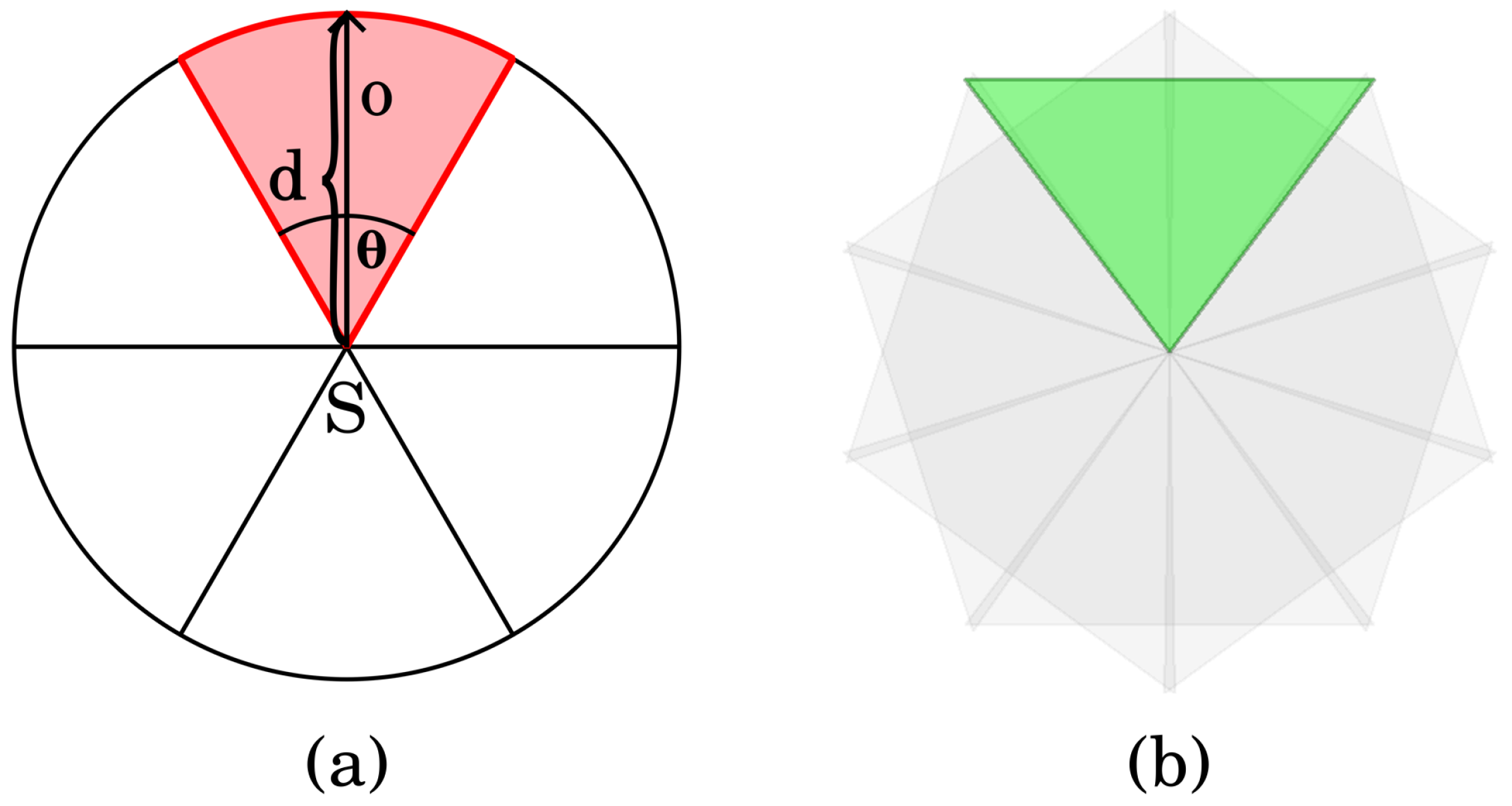
Figure 2.
The coverage graph of a permissible sector selection.
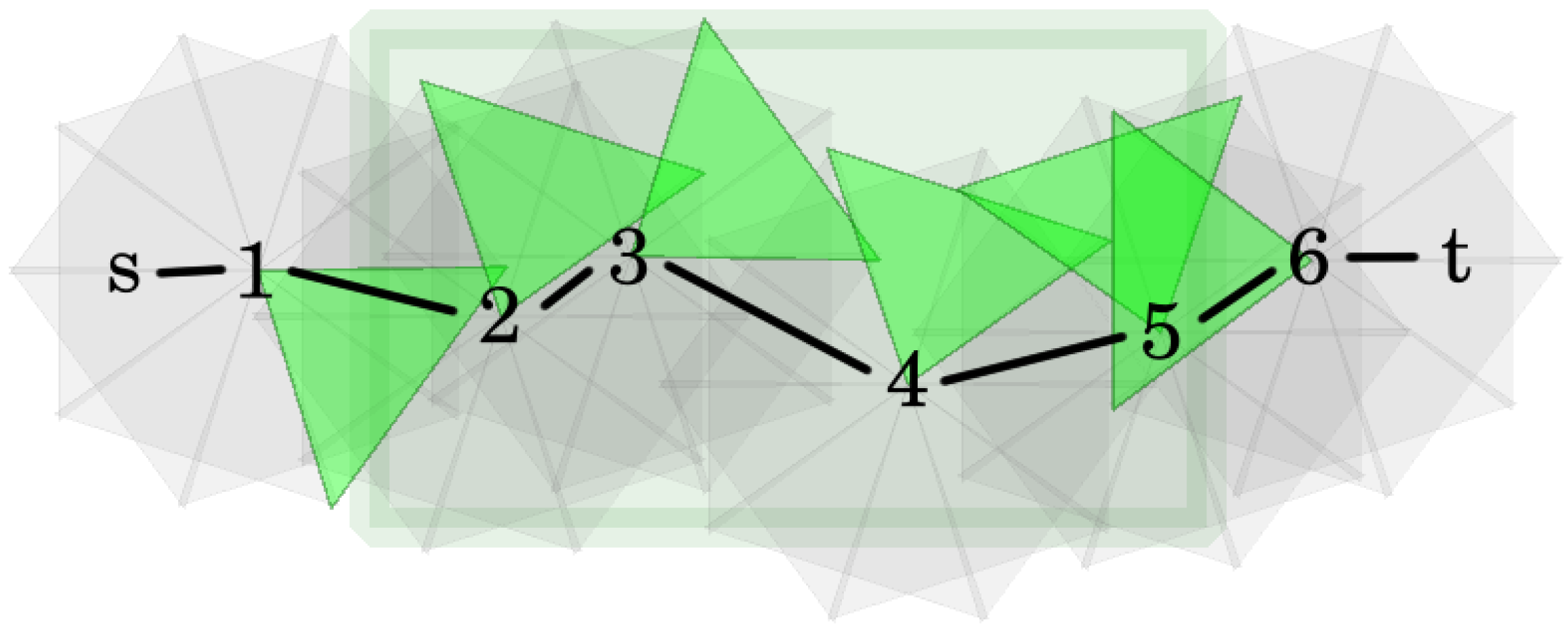
Figure 3.
A simple example for the transformation from a coverage graph to the corresponding network graph.
Figure 3.
A simple example for the transformation from a coverage graph to the corresponding network graph.
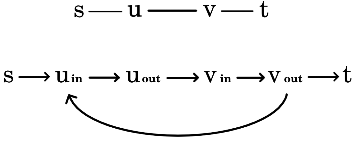
Figure 4.
(a) An example for horizontal clusters. (b) An example for vertical clusters.
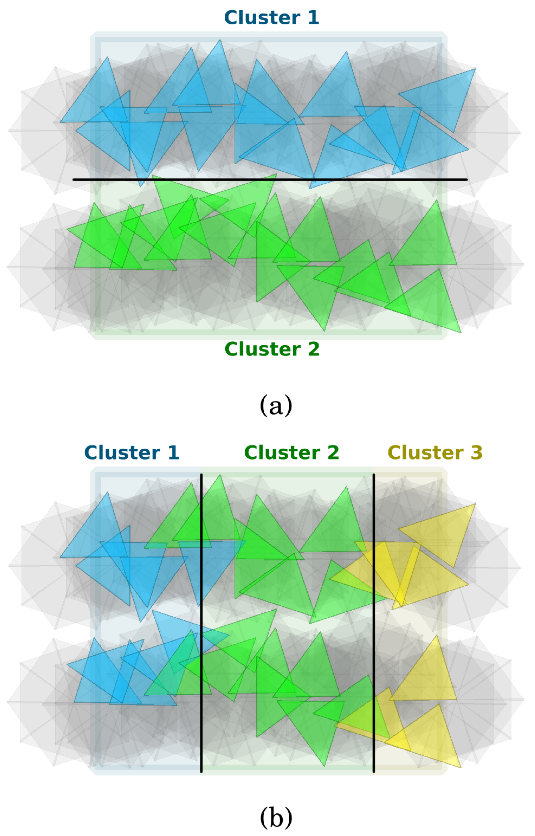
Figure 5.
(a) An example for how line segments are used to form the backbone of vertical clusters. (b) Adding multiple line segments to a vertical cluster. (c) Merging the source and sink nodes.
Figure 5.
(a) An example for how line segments are used to form the backbone of vertical clusters. (b) Adding multiple line segments to a vertical cluster. (c) Merging the source and sink nodes.
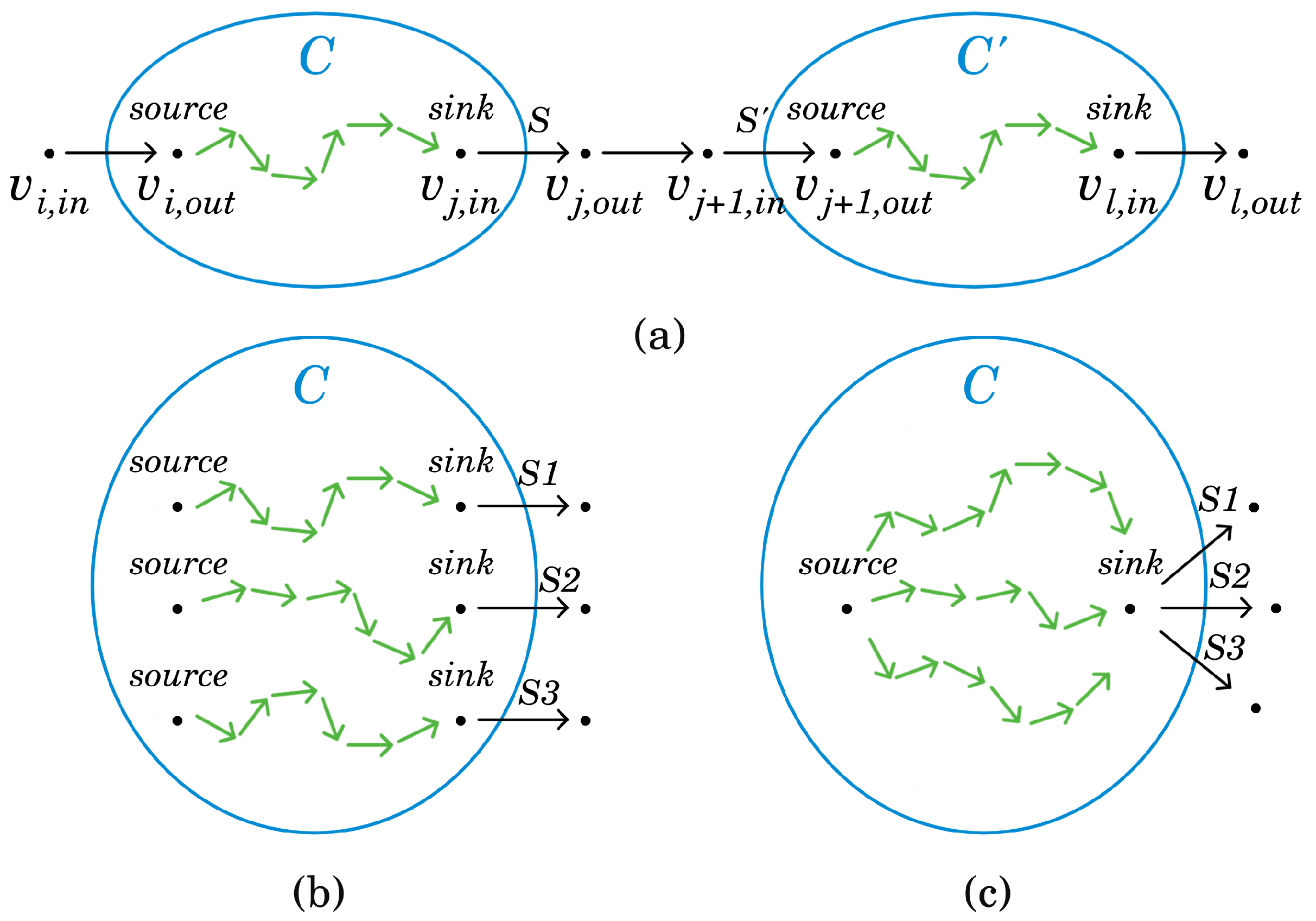
Figure 6.
An example when does not return an optimal result. (a) Sector. (b) Network graph.
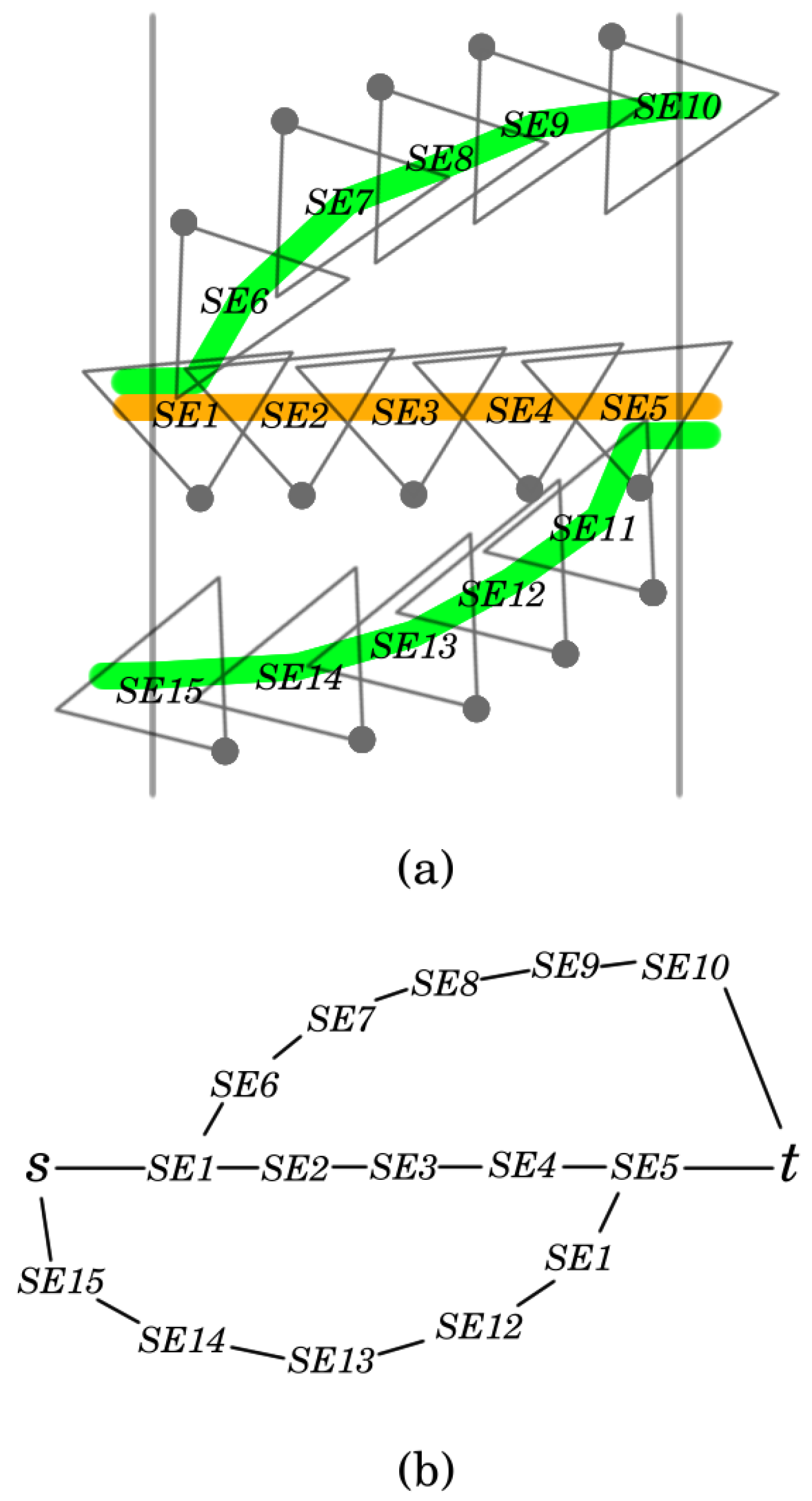

Table 1.
The result of comparing the outputs of and in 102 random scenarios.
| Greedy | 1 | 2 | 3 | 4 |
|---|---|---|---|---|
| ILP | ||||
| 1 | 2 | 0 | 0 | 0 |
| 2 | 3 | 8 | 0 | 0 |
| 3 | 0 | 14 | 14 | 0 |
| 4 | 0 | 6 | 28 | 6 |
| 5 | 0 | 0 | 4 | 17 |
Table 2.
Results for the MTCBC-1 problem.
| Omniscient | Only-camera | |||
|---|---|---|---|---|
| Algorithm | Avg tracking | Avg coverage | Avg tracking | Avg coverage |
| Baseline | 0.4082 | 0.4317 | 0.4082 | 0.4317 |
| Optimal | 0.9207 | 0.9362 | 0.6043 | 0.6357 |
| Horizontal | - | - | - | - |
| Vertical | 0.8707 | 0.9009 | 0.6001 | 0.6380 |
| Greedy | 0.8073 | 0.8731 | 0.7079 | 0.7926 |
Table 3.
Results for the MTCBC-2 problem.
| Omniscient | Only-camera | |||
|---|---|---|---|---|
| Algorithm | Avg tracking | Avg coverage | Avg tracking | Avg coverage |
| Baseline | 0.5101 | 0.4812 | 0.5101 | 0.4812 |
| Optimal | 0.9159 | 0.9243 | 0.8219 | 0.7919 |
| Horizontal | 0.9114 | 0.9246 | 0.6506 | 0.6845 |
| Vertical | 0.8501 | 0.8528 | 0.5719 | 0.5988 |
| Greedy | 0.7652 | 0.7900 | 0.6702 | 0.7193 |
Table 4.
Runtime of the algorithms.
| Omniscient | Only-camera | |
|---|---|---|
| Optimal | 100% | 100% |
| Horizontal | 55.2% | 38.5% |
| Vertical | 40.8% | 27.8% |
| Greedy | 6.9% | 6.6% |
Disclaimer/Publisher’s Note: The statements, opinions and data contained in all publications are solely those of the individual author(s) and contributor(s) and not of MDPI and/or the editor(s). MDPI and/or the editor(s) disclaim responsibility for any injury to people or property resulting from any ideas, methods, instructions or products referred to in the content. |
© 2024 by the authors. Licensee MDPI, Basel, Switzerland. This article is an open access article distributed under the terms and conditions of the Creative Commons Attribution (CC BY) license (http://creativecommons.org/licenses/by/4.0/).
Copyright: This open access article is published under a Creative Commons CC BY 4.0 license, which permit the free download, distribution, and reuse, provided that the author and preprint are cited in any reuse.


