Submitted:
15 August 2023
Posted:
16 August 2023
You are already at the latest version
Abstract
Abstract: The traditional model of closed circuit ball milling systems has been used for several decades, however, if the classifier of the closed circuit ball mill system performs the duties of both pre-classification and check-classification, the characterization error of the traditional model is large. To address this problem, a new model is obtained by modifying and supplementing the traditional one. The most important feature of the new model compared to the traditional model is that the circulating load is considered to be the fresh feed for the entire system rather than the ball mill. The error between the slurry level height calculated using the traditional model and the actual is 52.31%, which is 13.77 times higher than that of the new model. When the relative capacity varies greatly, that of the ball mill calculated by the traditional model fluctuates between 0.95 and 1.15, while the new model is 0.6 to 1.4. The new model has a higher accuracy than the traditional model in characterizing the production status of the grinding system, which is of some significance for industrial production.
Keywords:
Closed circuit ball mill
; circulating load
; classification efficiency
; relative capacity of ball mills
; industrial applications
1. Introduction
Grinding is a pretreatment operation for mineral processing, and its main purpose is to crush large pieces of ore to the size needed for separation[1]. At the same time, the ball mill is the most energy-intensive operation in the ore processing plant because of its large operating power[2,3]. With the increasing severity of the greenhouse effect and the growing urgency to reach the carbon peak, milling is receiving more and more attention from researchers[4,5,6,7]. From laboratory batch grinding[8,9,10] to industrial ball mills[11,12,13], from single[14,15] to multiple minerals[16,17,18], from breakage rate function[19] to population balance model[20,21,22,23], scholars have invested a lot of effort in better characterizing and predicting grinding characteristics. For industrial ball mills, circulating load[24,25,26,27] and classification efficiency[28,29] are the two most important indicators to characterize their working condition.
Industrial ball mills are usually used in conjunction with classifiers, which play the role of preventing fine particles from entering the ball mill and controlling the size of the final product. With the wide application of classification equipment represented by hydrocyclones[30] and high-frequency screens[31], the working condition of classification equipment has received unprecedented attention, and a large number of models to characterize the working condition of classification equipment have emerged over time[30,32,33]. In all models, circulation load and classification efficiency are the two most important indicators, the former reflects the operation of the ball mill and the latter signals the efficiency of the classifier. For open circuit grinding[34,35], there is no disagreement with the calculation of the circulating load and classification efficiency, both of which can be characterized relatively accurately. However, for closed circuit grinding[28,36], the authors find that the existing calculation methods and models are not accurately characterized based on data from a large number of industrial grinding and classifying systems, and need to be revised and supplemented.
2. Theoretical background
2.1. Classification
Classification is an operation where particles are separated according to particle size. The two most common classification methods are screening and hydraulic classification. The high-frequency vibration sieve is the representative of the former method and the hydrocyclone is the representative of the latter. The process by which materials are separated into different particle sizes through one or more layers of the screen surface is called screening classification[31]. Hydraulic classification is the process of dividing a broad particle size class into a number of narrow size class products according to the different settling velocities of the frame in the moving medium[30]. The product of the grinding operation is a broad size mineral group, where the coarse size minerals do not meet the size requirements of the subsequent operation. At this time, the ball mill needs to be used with classification equipment to feed the material that meets the size requirements into the next process, and the material that does not meet the size requirements is returned to the ball mill for regrinding. According to the different functions of classification, it can be further divided into pre-classification and check-classification.
Pre-classification is to discharge the qualified particles in advance before entering the ball mill to avoid the transitional crushing of materials and thus improve the capacity of the ball mill and reduce energy consumption. For pre-classification, there is no circulating load because no material is returned to the ball mill.
Check-classification is to control the particle size of the discharged product after the material has been ground by the ball mill, and to return the coarse particles with unqualified particle size to the ball mill for regrinding, so as to ensure that the final product meets the particle size requirements of the subsequent operation.
2.2. Grinding circuit
Depending on the function of the classifier, the grinding circuit can be divided into open circuit ball milling and closed circuit ball milling. As shown in Figure 1(a), open circuit ball milling involves the grinding circuit in which the material is pre-discharged by the classification operation before entering the ball mill. It is characterized by a relatively small amount of material entering the ball mill, in which case the relative processing capacity of the ball mill is larger and the energy consumption per unit is lower. However, a certain number of coarse particles will be present in the final product of the open circuit ball milling, which will have an impact on the subsequent separation. As shown in Figure 1(b), the ball mill discharge enters the classification stage before going into separation, and the classification operation returns the unqualified particles to the ball mill for regrinding to form a closed circuit, which is called closed circuit ball milling. When the amount of returned material is large, the efficiency of the ball mill decreases and the energy consumption per unit increases significantly.
2.3. Circulating load and classification efficiency
The circulating load of the ball mill refers to the mass percentage of the return to the fresh feed (by solid). Circulating load is an important index of grinding and classifying system, which can directly reflect the instantaneous processing capacity of ball mills. It is directly related to the working condition of the ball mill and the classifier, usually the circulating load of the ball mill and the classifier is small when the working efficiency is high, and vice versa. The plant calculates the circulating load to determine if the grinding media needs to be replenished or the processing capacity needs to be changed.
Hydraulic classification is the process of dividing a broad particle size class into a number of narrow size class products according to the different settling velocities of the frame in the moving medium under centrifugal and drag forces. The classification used in this thesis refers to the use of hydrocyclones as classification equipment to obtain a finer size overflow and a coarser size underflow. The classification efficiency refers to the mass of solids smaller than a certain size in the overflow as a percentage of the total weight of solids of that size. Both it and the circulating load are important parameters in the analysis of the operation of a closed circuit ball mill, and there is also a functional relationship between the two that one can be transformed into the other.
3. Mathematical models and Methodology
Numerous studies have indicated that the particle size characteristics of the ground product from short time grinding are consistent with first-order grinding kinetics[37,38,39,40], implying that the rate of fines production () equals to the rate of the coarse () breakage. The first-order grinding kinetics can be written as the following equation:
where is the amount of coarse material, the grinding rate constant, and is the grinding time.
3.1. Sole function of check-classification (the traditional model)
As shown in Figure 2, when the feed ore in a closed circuit ball mill system is first fed into the ball mill and then the discharge enters the classifier, the classifier plays only the role of check-classification. The overflow from the classifier is the final product and the underflow is returned to the ball mill for regrinding. In this case, the ball mill capacity is related to both the circulating load (and classification efficiency (.
Assuming that there is only coarse material in the mill feed (new feed), the total mass of solids in the ball mill discharge can be derived according to the mass conservation equation of solids as:
According to Jankovic's[29] calculations, the fractions of coarse material in the feed ( and discharge ( of the ball mill can be derived as:
Assuming that the fraction of coarse material in the mill load () is the arithmetic mean of the fraction in the feed and product, according to the first order grinding kinetics, mill capacity can be expressed as:
Ultimately, the relative capacity of this closed circuit ball mill is:
where is the relative capacity, , are the circulating load and , are the classification efficiency under different milling circuit capacity (It is worth noting that Jankovic made a mistake in calculating this value by reversing the numerator and denominator, which has been corrected in this paper).
According to the material mass conservation it can be derived that the following relationship exists between the new feed Q of the ball mill, the ball mill discharge D, the overflow OF of the hydrocyclone and the underflow UF:
According to the conservation of mass of fine material, it is obtained that:
The circulating load refers to the ratio of the hydrocyclone underflow to the new feed to the ball mill:
The circulating load refers to the ratio of the hydrocyclone underflow to the new feed to the ball mill:
According to the definition of classification efficiency it is obtained that:
The following relationship exists between classification efficiency and circulating load:
where , and are the mass fraction of the underflow, classifier feed and overflow less than a specific size, respectively.
The calculation method and relationship between circulating load and classification efficiency described in closed grinding circuit with single check-classification has been used since 1968 when Hukki proposed it[3,29,41], regardless of the type of closed circuit ball mill (traditional model). The traditional model has been a key tool in guiding ball mill production for many years and is the cornerstone of grinding technology development. However, a deeper study of closed circuit grinding reveals that the simple extension of this model is not rigorous, especially for closed grinding circuit with pre-classification and check-classification.
3.2. Synergized functions of pre-classification and check-classification
When there is pre-classification and check-classification in closed circuit grinding, we need to modify and supplement the model. As shown in Figure 3(a), when the feed ore in closed circuit ball mill system is first fed into the classifier and then entering the ball mill, the classifier has role of both pre-classification and check-classification. Now, there are two models necessary to be analyzed in detail later. Model A works when the two roles of the classification equipment are analyzed separately, and then the parameters such as circulating load of classification are calculated (pre-classification has no circulating load). Model A could be viewed as an extension of the traditional model, but the shortcoming of the traditional one, which lies in guiding the industrial practice, still exists. Thus, model B is developed and referred to as the “new model” for the sake of comparison later. As shown in Figure 3(b), model B functions when the two roles of the classifier are considered as a whole to calculate its parameters such as circulating load and classification efficiency.
3.2.1. Model A (the extension of the traditional model)
Model A is based on the fact that although a classifier has both pre-classification and check-classification roles to play, there is no circulating load for pre-classification, so a separation is made for the classifier as shown in Figure 3(a). From the mass conservation of the solid of the feed and the discharge, it is obtained that:
where S1, S2 and S are the solid mass of the underflow of the pre-classification, check-classification and the whole classification operation, respectively; Q1, Q2, Q3 and Q are the solid mass of the overflow of the pre-classification, check-classification, ball mill discharge and the whole classification operation, respectively.
The total solid mass of the ball mill discharge is , and the mass of the fine particle in the feed of classifier is /E. The mass of fines in the underflow of check-classification is equal to the mass of fines in the classifier feed minus the mass of fines in the overflow, and its equation is expressed as:
The mass flow of the coarse material in the mill discharge is the difference between the total solids and the fine particle:
The total amount of the coarse material in the mill feed is:
Combining Equation (12)-(14), we can derive the fraction of coarse particles in the feed and the discharge of the ball mill as:
Assuming that the fraction of coarse material in the mill load is the arithmetic mean of the fraction in the feed and the product, according to the first order grinding kinetics, the mill capacity can be expressed as:
Ultimately, the relative capacity of this closed-circuit ball mill is:
where is the relative capacity, , are the circulating load and , are the classification efficiency under different milling circuit capacity.
Based on the mass conservation of the solid for a specific particle size in and out of the classifier, it can be concluded that:
After conversion, the circulating load is obtained as:
The following relationship exists between classification efficiency and circulating load:
where , and are the mass fraction of the underflow, classifier feed and overflow less than a specific size, respectively.
From the calculation results, it can be seen that model A actually also works for the closed circuit ball mill with solely the function of check-classification (Section 3.1). So, model A could be regarded as the extension of the traditional model, working for the closed circuit ball mill with the synergized functions of both pre-classification and check-classification.
3.2.2. Model B (the new model)
If the functions of the classifier are considered as a whole, then the total solid mass of the ball mill discharge is , and the mass of the fine particle in the feed of classifier is Q/E. The mass of fines in the ball mill feed is equal to the mass of fines in the classifier feed minus the mass of fines in the overflow, and its equation is expressed as:
The mass of the coarse particle in the mill feed is:
The mass of fines in the classifier feed is likewise the sum of the mass of fines in the new feed and ball mill discharge of the closed circuit ball mill system.
So, the mass of the fines in the ball mill discharge is:
The mass of the coarse particle in the ball mill discharge is:
where is the fraction of fine particles (particles with a size less than a specific particle size) in the fresh feed of the closed circuit ball mill system. Combining Equation (22)-(25) we can derive the fraction of coarse particles in the feed and the discharge of the ball mill as:
Assuming that the fraction of coarse material in the mill load is the arithmetic mean of the fraction in the feed and the product, according to the first order grinding kinetics, the mill capacity can be expressed as:
Ultimately, the relative capacity of this closed circuit ball mill is:
where and is the fraction of fine particles under different milling circuit capacity.
Based on the mass conservation of the solid for a specific particle size in and out of the classifier, it can be concluded that:
where is the mass of solids in the circulating load. The circulating load is the ratio of solids mass in the returned material to the new feed in the closed circuit ball mill system. Dividing each of the left and right terms of Equation (30) by Q, the circulating load is obtained as:
The classification efficiency is the mass percentage of fine particles in the overflow to the same size in the classifier feed:
The following relationship exists between classification efficiency and circulating load:
where , and are the mass fraction of the ball mill feed, ball mill discharge and overflow less than a specific size, respectively.
3.3. Methodology
To better illustrate the characteristics and differences between the two models, we summarize two very different mineral processing plants as examples. Case A is a mineral processing plant in Nanshan Mine, Anhui Province, China. Nanshan mine is typical of a closed circuit ball mill system where the classifier has two roles (fresh feed is fed to the classifier instead of the ball mill). The second stage ball mill model of Nanshan mine is MQY2736, and the second stage classifier is hydrocyclone model FX350, and their specific parameters are shown in Table 1. The volume of this ball mill is only about 20 m3, and the circulating load will increase significantly when the feed volume increases. Case A is a typical case of high circulating load that would be encountered in industrial production of a small ball mill, so it is used as the first case to compare the two models.
Case B is a mineral processing plant in Longqiao Mine, Anhui Province, China. The second stage ball mill of Longqiao mine is MQY3660 ball mill and the second stage classifier is high frequency screen, their specific parameters are shown in Table 2. The volume of the ball mill is about 60 m3, but there are two primary ball mills. The plant will decide whether to run two primary ball mills or only one according to production needs, which results in a very unstable amount of ore entering the secondary ball mill and large variations in the relative capacity of the ball mill. On the other hand, in contrast to Case A, the classification equipment in Case B is a high-frequency screen, which is known for its high classification efficiency. Case B is another industrial typical ball mill classification system with a high frequency screen as classification equipment, characterized by low circulating load and high classification efficiency.
Both Case A and Case B avail the most common closed circuit ball mill systems as shown in Figure 3(b), and they will be used in this paper to compare the differences between the two models.
4. Case Study
4.1. Case A: Larger circulating load
Nanshan Mine is a traditional magnetite processing plant, because of the early construction of the plant and the need to expand capacity, so the closed circuit ball mill system of the processing plant has a large circulating load. Figure 4 shows the size characteristics of the products in the closed circuit ball mill system of Nanshan Mine. It can be seen that the mass fraction of -0.075 mm particles in the discharge of secondary mill is 26.51%, but the value in the overflow has increased to 77.92%, indicating that the circulating load is seriously out of the conventional range.
This closed circuit ball mill system was closely tested, and the calculated results of statistical data, circulating load, and classification efficiency are summarized in Table 3. Although the same data were used, the circulating loads and classification efficiencies derived using the traditional model and the new model differed considerably. The difference in circulating load can reach a maximum of 597.78 percentage points, accounting for 62.36%; The difference in classification efficiency can reach a maximum of 23.82 percentage points, accounting for 57.03%. Since the calculation of the two models differs greatly, which model is the better fit for the situation of the site? In this paper, we will look for the answer to this question in terms of both the relative capacity of the ball mill and the actual operating condition.
4.1.1. Relative capacity
The mathematical model in Section 3 shows that the expressions of the two models regarding the relative capacity of the ball mills are:
The new model considers the classifying equipment as a whole and should not be viewed that it is divided into two classifying equipment with different roles. If not, it will not only lead to significant calculation errors but also make it impossible to calculate the classification efficiency for pre-classification. The biggest difference between the new model and the traditional one is the addition of the characteristic parameters of the new feed to the closed circuit ball mill system, which eliminates the fluctuation of the circulating load and classification efficiency due to the fluctuation of the particle size characteristics of the new feed.
Figure 5 and Figure 6 show the calculation results using the traditional model and the new model, respectively. The calculations of the traditional model show a classification efficiency of about 60% for stable production, which decreased to about 40% at higher circulating loads. The relative capacity of the ball mill ranged from 0.95 to 1.15, indicating that the fluctuations in the capacity of the ball mill were not significant. The calculations of the new model show a classification efficiency of about 65% for stable production, which decreased to about 55% at higher circulating loads.
From the performance of classification equipment and common sense of ball mill industrial production, the classification efficiency of the same classification equipment will not change significantly when there is no significant change in the particle size characteristics of the new feed ore and the work state (like flow, pressure). The classification efficiency calculated with the traditional model appeared two concentration points, 65% and 50%, respectively. However, the classification efficiency calculated using the new model is basically distributed around 65%, so from this point of view, the calculation results of the new model are more fitting.
The relative capacity of the ball mill should increase significantly when the circulating load of the closed circuit ball mill system is close to 1000%, while the highest relative capacity in the traditional model is less than 1.10, so the new model is also more reasonable from this point of view.
4.1.2. Actual operating condition
The ball mill used in Nanshan Mine is MQY2736 ball mill, the diameter (R) of the ball mill is 2.7 m and the length (L) is 3.6 m. The internal liner of the ball mill is calculated as 0.1 m, then the volume of the ball mill is:
From the mathematical models in Section 3, it is known that the two models regarding the circulating load are calculated as:
The grinding media filling rate of this ball mill is 40%, assuming that the initial state of the ball mill slurry can exactly fill the space between the media, the remaining volume is:
Figure 7 shows a schematic cross-section of a ball mill, where is the radius of the ball mill, and is the height of the slurry level in the ball mill. Through the spatial geometry calculation, the relationship between the volume of new feed slurry in the ball mill and the slurry height in the ball mill can be obtained as follows:
where V is the volume of the newly fed slurry, which is the sum of the volumes of solids () and liquids () in the newly fed slurry.
The ball mill has a throughput of 60 t/h and the mass concentration of the slurry 70%. It can be seen from Table 3 that the circulating load calculated using the traditional model is 958.59% for larger, the density of magnetite is 4.85 t/m3. In the laboratory batch grinding process, keeping all operating parameters the same as the industrial reality, it was found that the fineness obtained by grinding 1min is similar to the industrial reality, so we assume that the industrial time for the pulp to pass through the ball mill is about 1min. If the time for the pulp to pass through the ball mill is 1 min, the volume of solids and liquid in the new feed is:
Bringing the result of Equation (39) into Equation (36) yields a slurry height of 1.98 m in the ball mill. The same industrial test data with the new model calculates a circulating load of 360.81%. Following the same calculation method yields:
Bringing the result of Equation (42) into Equation (36) yields a slurry height of 1.45 m in the ball mill. When the ball mill is running, some of the steel balls and slurry will be in the throwing state, which will cause the cross-sectional slurry height to decrease. Figure 8(a) shows the actual situation in the industrial site at that time, and Figure 8(b) shows the height corresponding to the height calculated by the two models in the ball mill. The distance from the top of the back of the ball mill to the horizontal center axis is 1300mm, and the height of the discharge liquid from the actual observation is almost exactly at the position of the horizontal center axis of the ball mill. The height of the discharge level calculated by the traditional model for the circulating load is 1980mm, indicating a distance of 620mm from the top of the ball mill interior, and similarly the distance obtained by the new model is 1250mm. From the above data, it is easy to conclude that the calculation error of the traditional model is 52.31%, while the calculation error of the new model is only 3.8%. The error of the discharge level height calculated by the traditional model is 13.77 times higher than that of the new model. It can be seen that the height calculated using the traditional model is much higher than the actual height, indicating that the conventional model has non-negligible errors in characterizing closed circuit ball mill systems with large circulating loads. This error can cause bias to the site staff in determining the ball mill operation status and in making related decisions, which ultimately affects production. On the contrary, the new model shows a high fit to the actual production situation and is instructive for the production of closed circuit ball mills with high circulating loads.
4.2. Case B: Large variation in relative capacity
Like Nanshan Mine, Longqiao Mine is a typical magnetite ore processing plant and has the same closed circuit ball mill system. The difference is that the classification equipment in the closed circuit ball mill system of Longqiao Mine is a high-frequency screen, which is characterized by high classification efficiency. However, the classification efficiency of the high-frequency screen will be significantly reduced when the throughput is too large to affect industrial production, so the circulating load is basically controlled below 300% during production. In addition, this closed circuit ball mill system sometimes handles material from two primary ball mills at the same time, so its ball mill relative capacity varies greatly.
Figure 9 shows the size characteristics of the products in the closed circuit ball mill system of Longqiao Mine. It can be seen that the mass fraction of -0.075 mm particles in the discharge was 54.50% and the value in the overflow was just 73.55%, indicating a circulating load much less than Case A.
This closed circuit ball mill system was closely tested, and the calculated results of statistical data, circulating load, and classification efficiency are summarized in Table 4. The circulating loads calculated by both models did not exceed 300% and were within 100% most of the time. The difference between the circulating loads calculated by the two models is significantly smaller compared to Case A, but when the circulating load is 8.24% (conventional model), the error between the two is as high as 494.25%. The reason for this phenomenon is that the circulating load value calculated by the traditional model tends to be zero, meaning that there is almost no return material, not in line with the production reality.
Figure 10 shows the calculation results using the traditional model. The relative capacity of the ball mill calculated by the traditional model without significant fluctuation is between 0.95 and 1.15, which is very close to Case A. However, the ball mill throughput in Case B varies greatly, and the relative capacity of the ball mill should have a large fluctuation. It can be seen that the traditional model has limitations in the characterization of the relative capacity of the ball mill when the passing capacity of the ball mill varies greatly, and cannot correctly reflect the working condition of the ball mill. Worse still, the data points derived from the traditional model do not have any distribution pattern and cannot be fitted by the traditional model.
Figure 11 shows the calculation results using the new model. The relative capacity of the ball mill calculated with the new model is between 0.6 and 1.4, which is more in line with the actual situation where the throughput of the ball mill varies greatly. When the throughput of the ball mill is lower, the ball mill processes less ore per unit time and the discharge gets finer, which helps to improve the classification efficiency. This is verified in the new model, where the classification efficiency is as high as 95% when the circulation load is below 100%, indicating that the new model can more accurately predict and characterize large variations in the relative capacity of the ball mill.
From the mathematical models in Section 3, it can be concluded that the relationship between circulating load and classification efficiency in both models is:
All data from the two cases were aggregated and characterized in Figure 12 and Figure 13 for the circulating load and classification efficiency relationships of the two models, respectively. The circulating load and classification efficiency are consistent with the Hukki model, whether calculated by the traditional model or the new model. It is shown that both models can better characterize the relationship between circulating load and classification efficiency, although there are deviations in the characterization about the relative capacity and actual operation of the ball mill.
5. Conclusion
When the role of the classifier in a closed circuit ball mill system is only to pre-classify, the traditional model calculates the circulating load and classification efficiency with a high degree of accuracy. However, when the classifier plays the role of both pre-classification and check-classification, the traditional model does not take into account the changes in the size characteristics of the fresh feed, resulting in great characterization errors. Therefore, in this paper, based on the traditional model, the influence of the particle size characteristics of the fresh feed is taken into account to obtain a new mathematical model of the closed circuit ball mill system. The new model has the following advantages over the traditional one:
- When the particle size characteristics of the new feed to the closed circuit grinding and classifying system and the operating parameters of the classifying equipment are not changed, the classification efficiency does not change significantly. The classification efficiencies calculated with the new model are basically around 65%, while two concentrations of 65% and 50% occur with the traditional model. Therefore, the classification efficiency characterization of the new model is more accurate than that of the traditional model in this case.
- The height of the ore pulp level inside the ball mill at the same moment is positively correlated with the circulating load. When the circulating load of the closed circuit grinding and classifying system is large, the distance of the pulp liquid level from the internal top of the ball mill calculated by the traditional model has an error of 3.8% from the actual one. And the calculation error of the traditional model is 52.31%, which is 13.77 times of the traditional model.
- When the relative capacity of the closed circuit ball mill system varies greatly, that of the ball mill calculated by the traditional model fluctuates between 0.95 and 1.15, while the new model is 0.6 to 1.4. That is to say, the new model is more responsive to the actual production situation than the traditional model, and is more significant in guiding the industrial practice.
Consequently, when the classifier in a closed circuit ball milling system performs two functions of pre-classification and check-classification, the characterization of ball mill operating conditions is more accurate using the new model. The new model is equivalent to a modification and supplement of the traditional one.
References
- Norgate, T.; Haque, N. Energy and greenhouse gas impacts of mining and mineral processing operations. J. Clean. Prod. 2010, 18, 266–274. [Google Scholar] [CrossRef]
- Ghalandari, V.; Esmaeilpour, M.; Payvar, N.; Reza, M.T. A case study on energy and exergy analyses for an industrial-scale vertical roller mill assisted grinding in cement plant. Adv. Powder Technol. 2021, 32, 480–491. [Google Scholar] [CrossRef]
- Fang, X.; Wu, C.; Liao, N.; Yuan, C.; Xie, B.; Tong, J. The first attempt of applying ceramic balls in industrial tumbling mill: A case study. Miner. Eng. 2022, 180, 107504. [Google Scholar] [CrossRef]
- Fang, X.; Wu, C.; Yuan, C.; Liao, N.; Chen, Z.; Li, Y.; Lai, J.; Zhang, Z. Can ceramic balls and steel balls be combined in an industrial tumbling mill? Powder Technol. 2022, 412. [Google Scholar] [CrossRef]
- Zhang, X.; Qin, Y.; Jin, J.; Li, Y.; Gao, P. High-efficiency and energy-conservation grinding technology using a special ceramic-medium stirred mill: A pilot-scale study. Powder Technol. 2021, 396, 354–365. [Google Scholar] [CrossRef]
- Gupta, V. Energy absorption and specific breakage rate of particles under different operating conditions in dry ball milling. Powder Technol. 2019, 361, 827–835. [Google Scholar] [CrossRef]
- Gupta, V. Validation of an energy–size relationship obtained from a similarity solution to the batch grinding equation. Powder Technol. 2013, 249, 396–402. [Google Scholar] [CrossRef]
- Faria, P.M.C.; Rajamani, R.K.; Tavares, L.M. Optimization of Solids Concentration in Iron Ore Ball Milling through Modeling and Simulation. Minerals 2019, 9, 366. [Google Scholar] [CrossRef]
- Zhao, R.; Han, Y.; He, M.; Li, Y. Grinding kinetics of quartz and chlorite in wet ball milling. Powder Technol. 2017, 305, 418–425. [Google Scholar] [CrossRef]
- Liu, S.; Li, Q.; Song, J. Study on the grinding kinetics of copper tailing powder. Powder Technol. 2018, 330, 105–113. [Google Scholar] [CrossRef]
- Mulenga, F.K. Sensitivity analysis of Austin's scale-up model for tumbling ball mills — Part 1. Effects of batch grinding parameters. Powder Technol. 2017, 311, 398–407. [Google Scholar] [CrossRef]
- Mulenga, F.K. Sensitivity analysis of Austin's scale-up model for tumbling ball mills — Part 2. Effects of full-scale milling parameters. Powder Technol. 2017, 317, 6–12. [Google Scholar] [CrossRef]
- Mulenga, F.K. Sensitivity analysis of Austin's scale-up model for tumbling ball mills – Part 3. A global study using the Monte Carlo paradigm. Powder Technol. 2017, 322, 195–201. [Google Scholar] [CrossRef]
- Yuan, C.; Wu, C.; Fang, X.; Liao, N.; Tong, J.; Yu, C. Effect of Slurry Concentration on the Ceramic Ball Grinding Characteristics of Magnetite. Minerals 2022, 12, 1569. [Google Scholar] [CrossRef]
- Koleini, S.M.J.; Barani, K.; Rezaei, B. The Effect of Microwave Treatment on Dry Grinding Kinetics of Iron Ore. Miner. Process. Extr. Met. Rev. 2012, 33, 159–169. [Google Scholar] [CrossRef]
- Guo, W.; Han, Y.; Li, Y.; Tang, Z. Impact of ball filling rate and stirrer tip speed on milling iron ore by wet stirred mill: Analysis and prediction of the particle size distribution. Powder Technol. 2020, 378, 12–18. [Google Scholar] [CrossRef]
- Xie, W.; He, Y.; Ge, Z.; Shi, F.; Yang, Y.; Li, H.; Wang, S.; Li, K. An analysis of the energy split for grinding coal/calcite mixture in a ball-and-race mill. Miner. Eng. 2016, 93, 1–9. [Google Scholar] [CrossRef]
- Fuerstenau, D.; Phatak, P.; Kapur, P.; Abouzeid, A.-Z. Simulation of the grinding of coarse/fine (heterogeneous) systems in a ball mill. Int. J. Miner. Process. 2011, 99, 32–38. [Google Scholar] [CrossRef]
- Epstein, B. Logarithmico-Normal Distribution in Breakage of Solids. Ind. Eng. Chem. 1948, 40, 2289–2291. [Google Scholar] [CrossRef]
- Reid, K.J. A solution to the batch grinding equation Chemistry Engineering Science 1965, 20, 953-963.
- Venkataraman, K.; Fuerstenau, D. Application of the population balance model to the grinding of mixtures of minerals. Powder Technol. 1984, 39, 133–142. [Google Scholar] [CrossRef]
- Gupta, V. Population balance modeling approach to determining the mill diameter scale-up factor: Consideration of size distributions of the ball and particulate contents of the mill. Powder Technol. 2021, 395, 412–423. [Google Scholar] [CrossRef]
- Gupta, V. Effect of particulate environment on the grinding kinetics of mixtures of minerals in ball mills. Powder Technol. 2020, 375, 549–558. [Google Scholar] [CrossRef]
- Bond, F.C. Crushing-and-Grinding-Calculations. pdf. Additions and Revisions 1962.
- Barkhuysen, N.J. Implementing strategies to improve mill capacity and efficiency, with platinum references and case studies. 2010.
- Groenewald, J.d.V.; Coetzer, L.; Aldrich, C. Statistical monitoring of a grinding circuit: An industrial case study. Miner. Eng. 2006, 19, 1138–1148. [Google Scholar] [CrossRef]
- Pural, Y.E.; Çelik, M.; Ozer, M.; Boylu, F. Effective circulating load ratio in mill circuit for milling capacity and further flotation process - lab scale study. Physicochem. Probl. Miner. Process. 2022, 58. [Google Scholar] [CrossRef]
- Telichenko, V.I.; Sharapov, R.R.; Lozovaya, S.Y.; Skel, V.I. Analysis of the efficiency of the grinding process in closed circuit ball mills. MATEC Web Conf. 2016, 86, 04040. [Google Scholar] [CrossRef]
- Jankovic, A.; Valery, W. Closed circuit ball mill – Basics revisited. Miner. Eng. 2013, 43-44, 148–153. [Google Scholar] [CrossRef]
- Nageswararao, K.; Wiseman, D.; Napier-Munn, T. Two empirical hydrocyclone models revisited. Miner. Eng. 2004, 17, 671–687. [Google Scholar] [CrossRef]
- Dündar, H. Investigating the benefits of replacing hydrocyclones with high-frequency fine screens in closed grinding circuit by simulation. Miner. Eng. 2020, 148, 106212. [Google Scholar] [CrossRef]
- Lee, W.; Jung, M.; Han, S.; Park, S.; Park, J.-K. Simulation of layout rearrangement in the grinding/classification process for increasing throughput of industrial gold ore plant. Miner. Eng. 2020, 157, 106545. [Google Scholar] [CrossRef]
- le Roux, J.D.; Steinboeck, A.; Kugi, A.; Craig, I.K. Steady-state and dynamic simulation of a grinding mill using grind curves. Miner. Eng. 2020, 152, 106208. [Google Scholar] [CrossRef]
- Mulenga, F.; Bwalya, M. Application of the attainable region technique to the analysis of a full-scale mill in open circuit. J. South. Afr. Inst. Min. Met. 2015, 115, 729–740. [Google Scholar] [CrossRef]
- Mulenga, F.K.; Mkonde, A.A.; Bwalya, M.M. Effects of load filling, slurry concentration and feed flowrate on the attainable region path of an open milling circuit. Miner. Eng. 2016, 89, 30–41. [Google Scholar] [CrossRef]
- Mackinnon, S.; Yan, D.; Dunne, R. The interaction of flash flotation with closed circuit grinding. Miner. Eng. 2003, 16, 1149–1160. [Google Scholar] [CrossRef]
- V.K.Gupta. The Estimation of Bate and Breakage Distribution P ammeters from Batch Grinding Data for a Complex Pyritic Ore Using a Back-Calculation Method. Powder Technology 1981, 28, 97-106.
- Capece, M.; Bilgili, E.; Dave, R. Identification of the breakage rate and distribution parameters in a non-linear population balance model for batch milling. Powder Technol. 2011, 208, 195–204. [Google Scholar] [CrossRef]
- Bilgili, E.; Scarlett, B. Population balance modeling of non-linear effects in milling processes. Powder Technol. 2005, 153, 59–71. [Google Scholar] [CrossRef]
- Austin, L.; Luckie, P. Note on influence of interval size on the first-order hypothesis of grinding. Powder Technol. 1971, 4, 109–110. [Google Scholar] [CrossRef]
- Hukki. R.T. A quantitative investigation of the closed grinding circuit. Transactions SME 1968, 241 (December), 482–487.
Figure 1.
Open circuit and closed circuit ball milling.
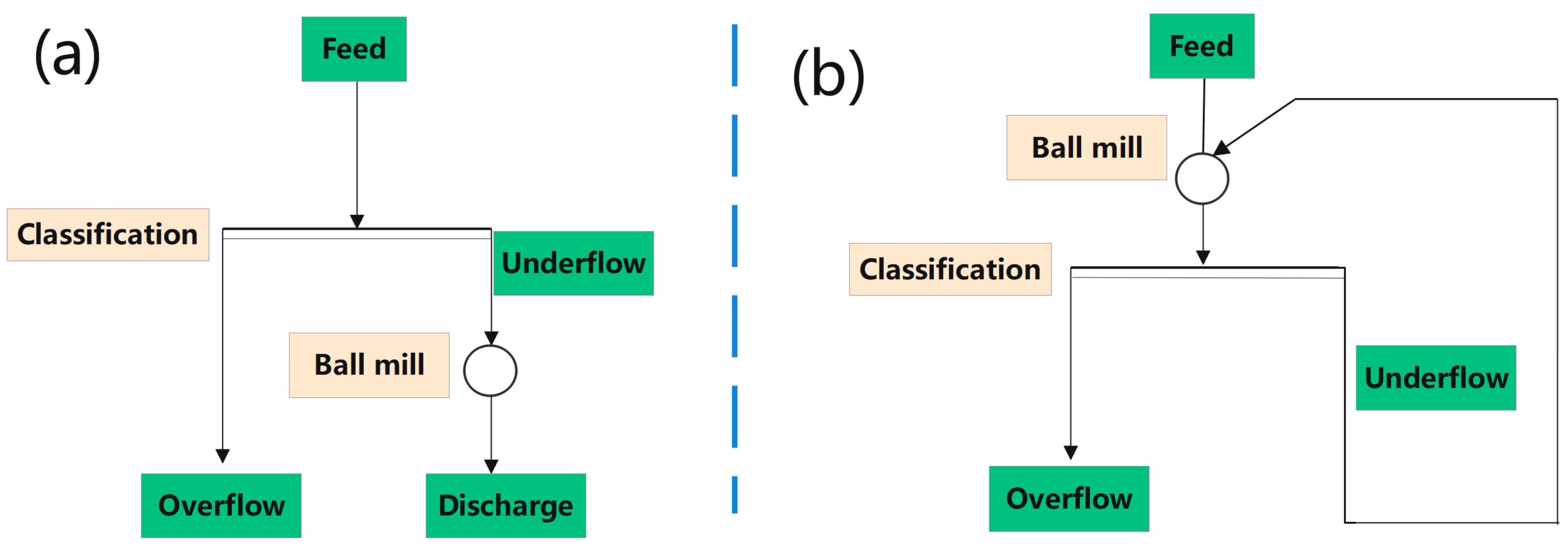
Figure 2.
Flow chart of the first type of closed circuit ball mill.
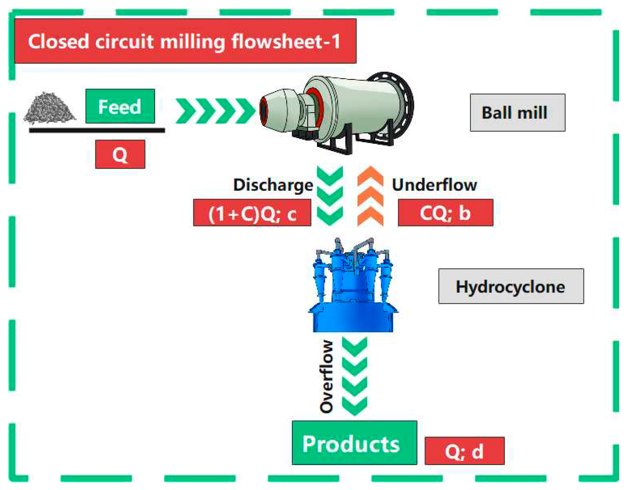
Figure 3.
Flow chart of the second type of closed circuit ball mill.
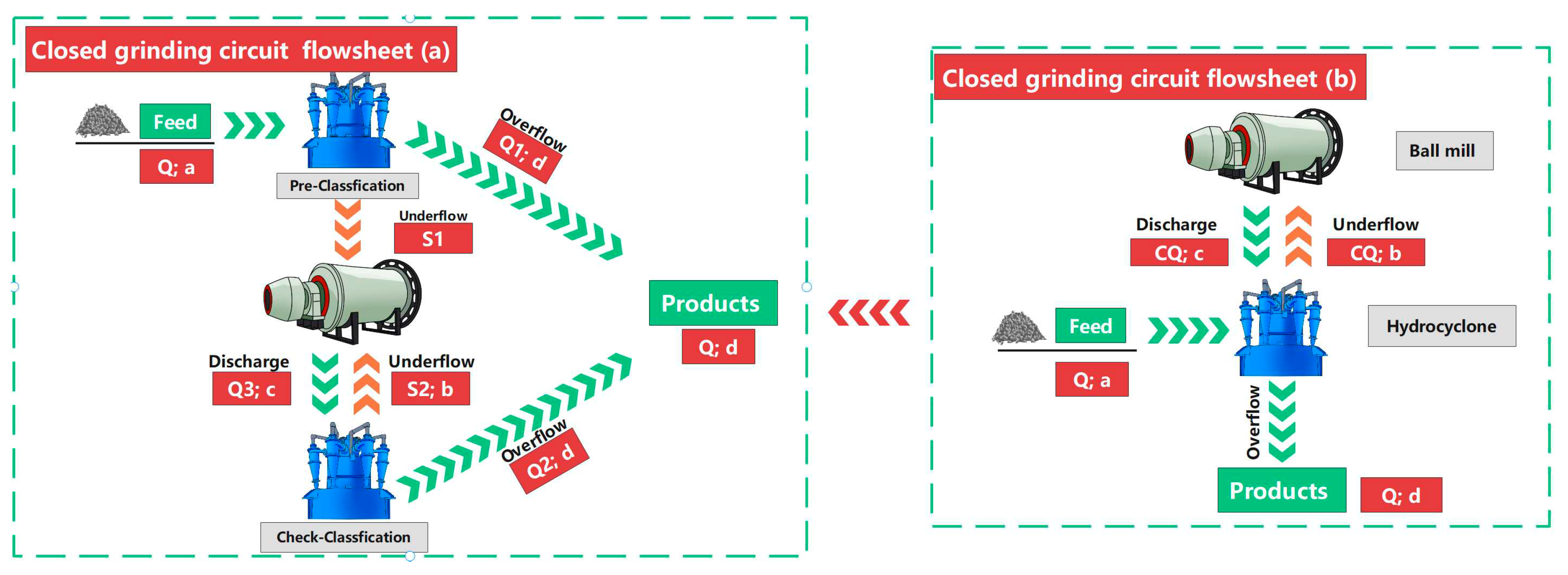
Figure 4.
Particle size characteristics of each product in the closed circuit ball mill system of Nanshan Mine.
Figure 4.
Particle size characteristics of each product in the closed circuit ball mill system of Nanshan Mine.
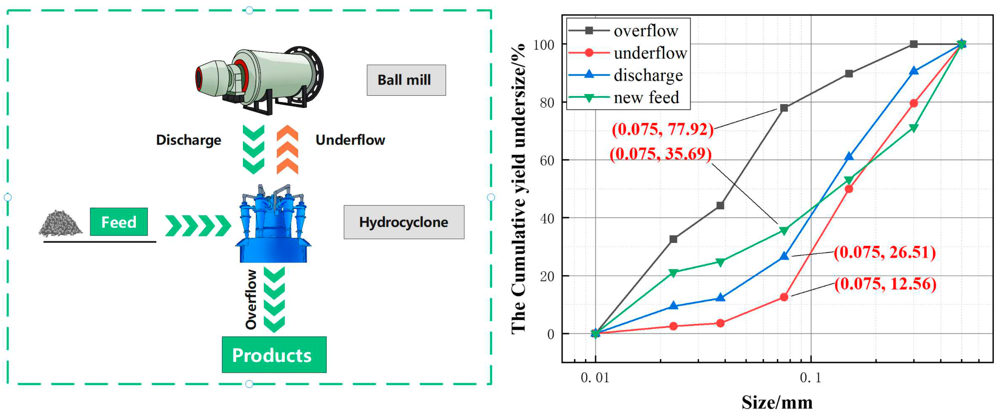
Figure 5.
Calculation results of the traditional model of Nanshan Mine.
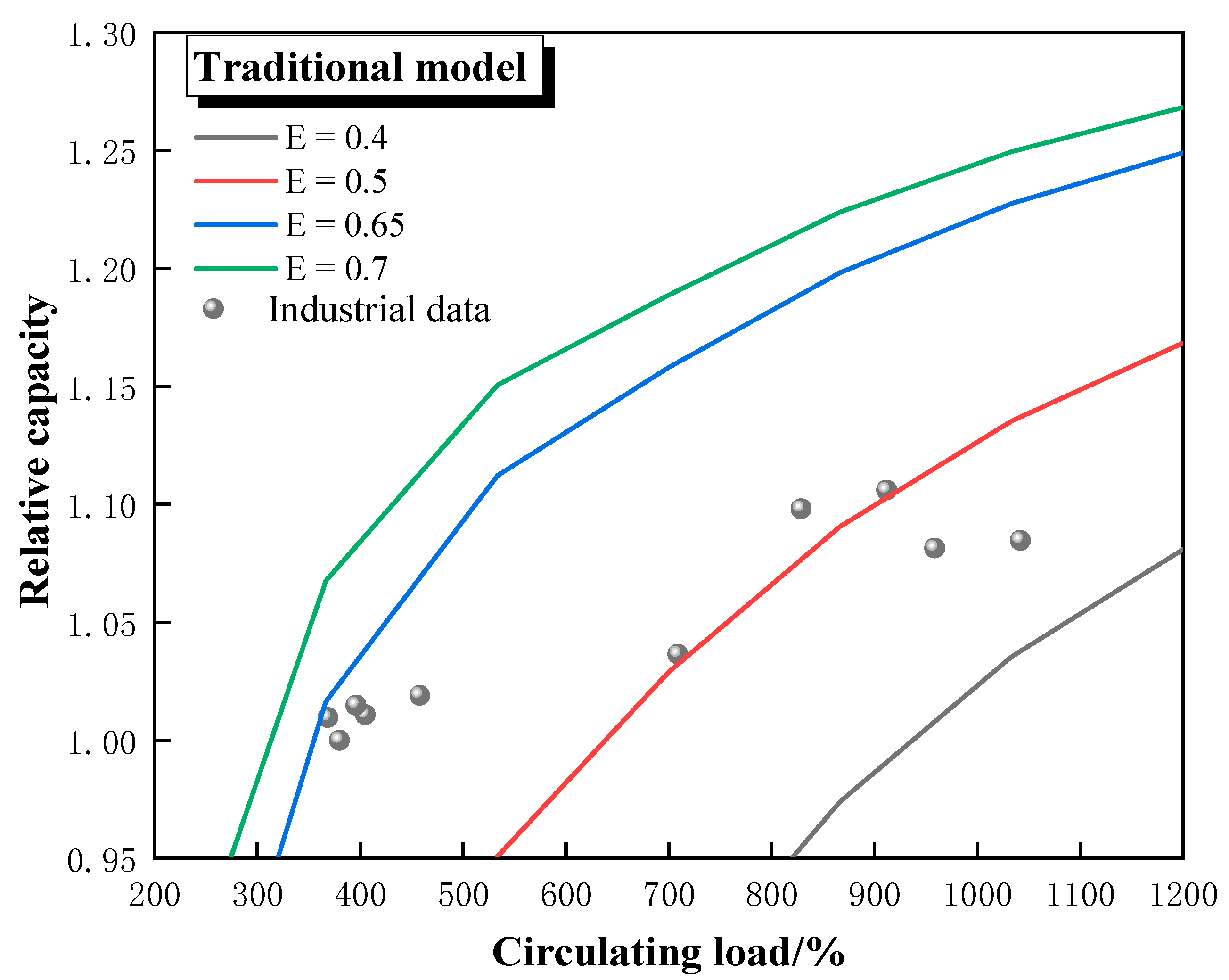
Figure 6.
Calculation results of the new model of Nanshan Mine.
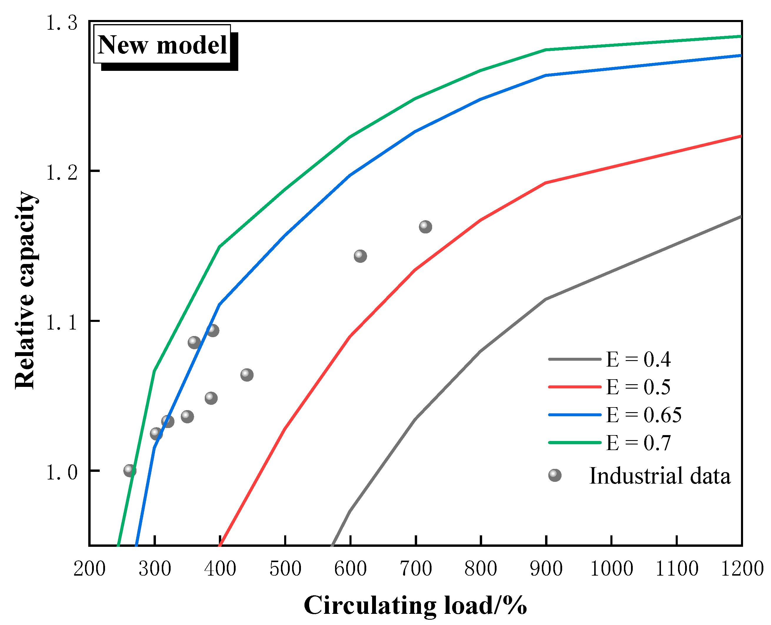
Figure 7.
Schematic diagram of ball mill cross section.
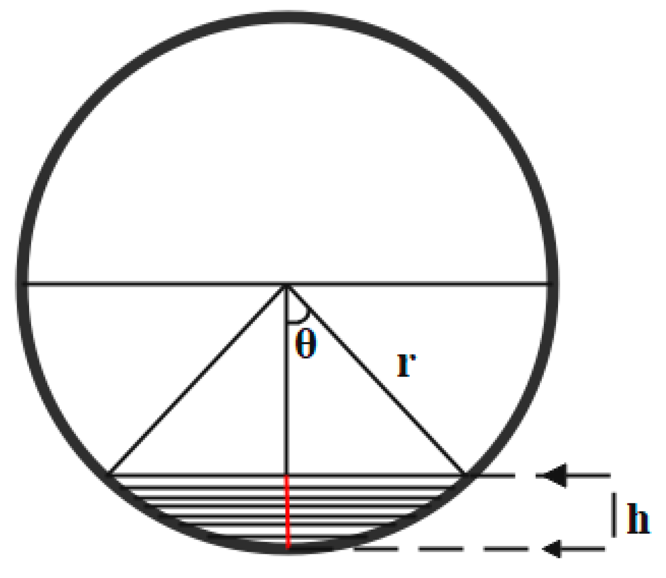
Figure 8.
Actual situation on industrial site.
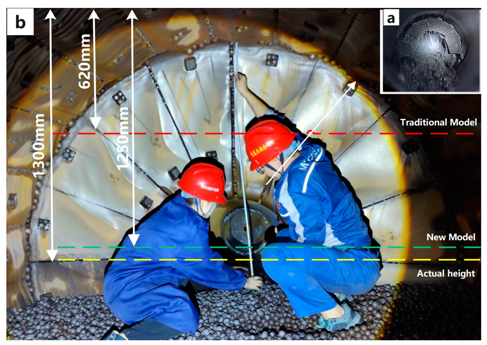
Figure 9.
Particle size characteristics of each product in the closed circuit ball mill system of Longqiao Mine.
Figure 9.
Particle size characteristics of each product in the closed circuit ball mill system of Longqiao Mine.
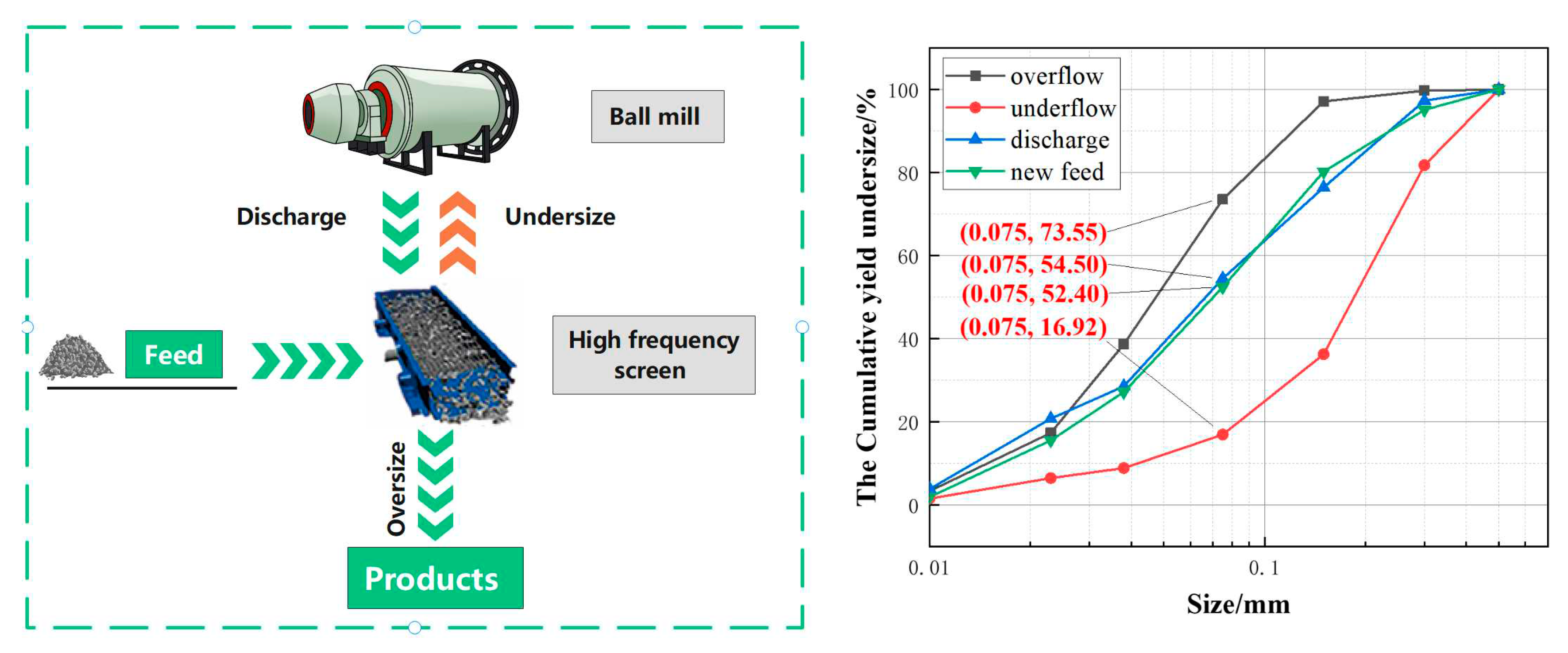
Figure 10.
Calculation results of traditional model of Longqiao Mine.
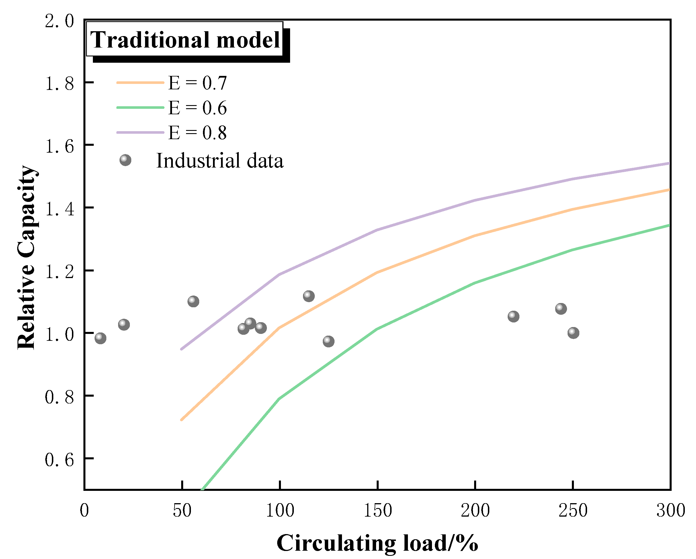
Figure 11.
Calculation results of the new model of Longqiao Mine.
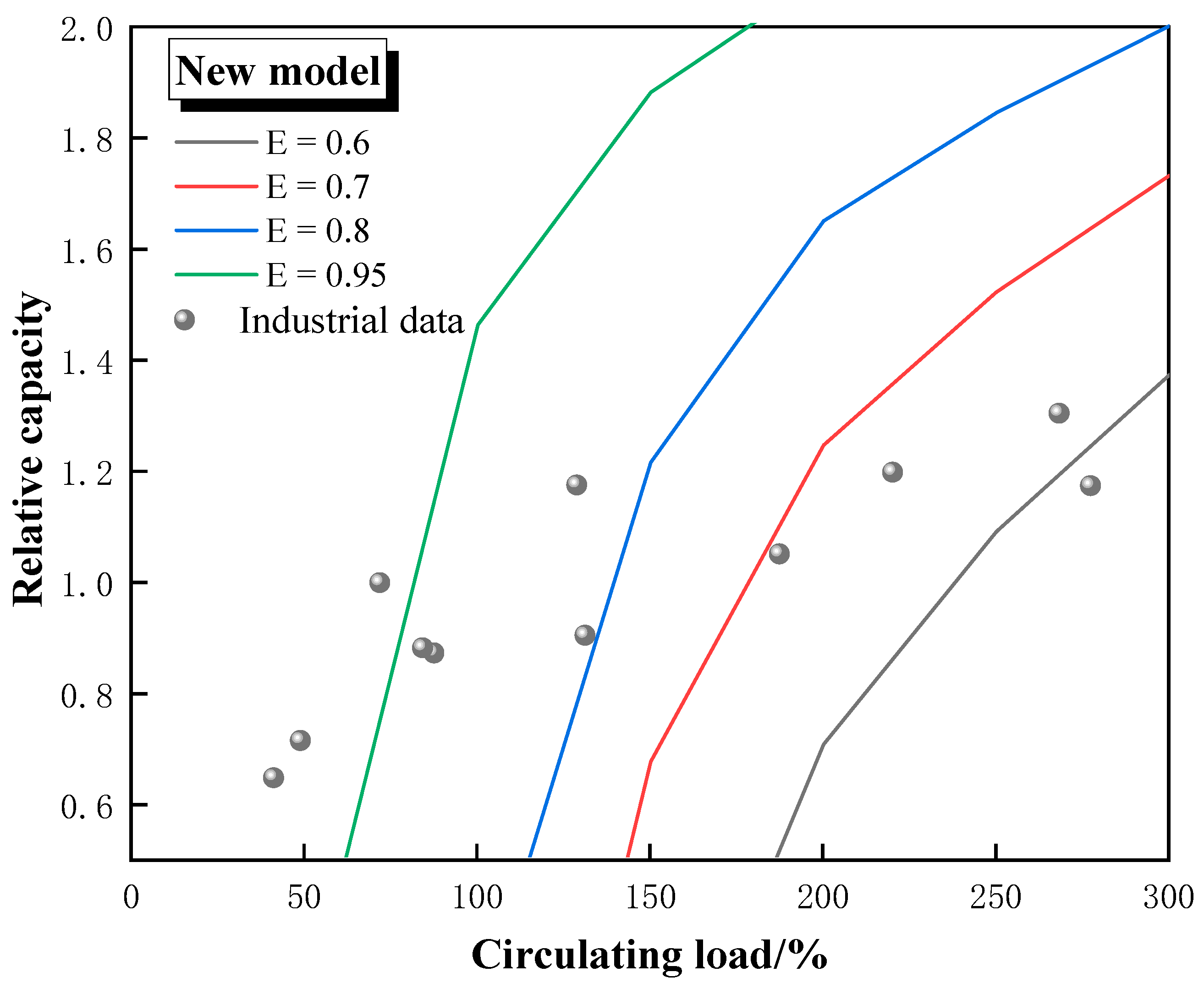
Figure 12.
The relationship between circulating load and classification efficiency in the traditional model.
Figure 12.
The relationship between circulating load and classification efficiency in the traditional model.
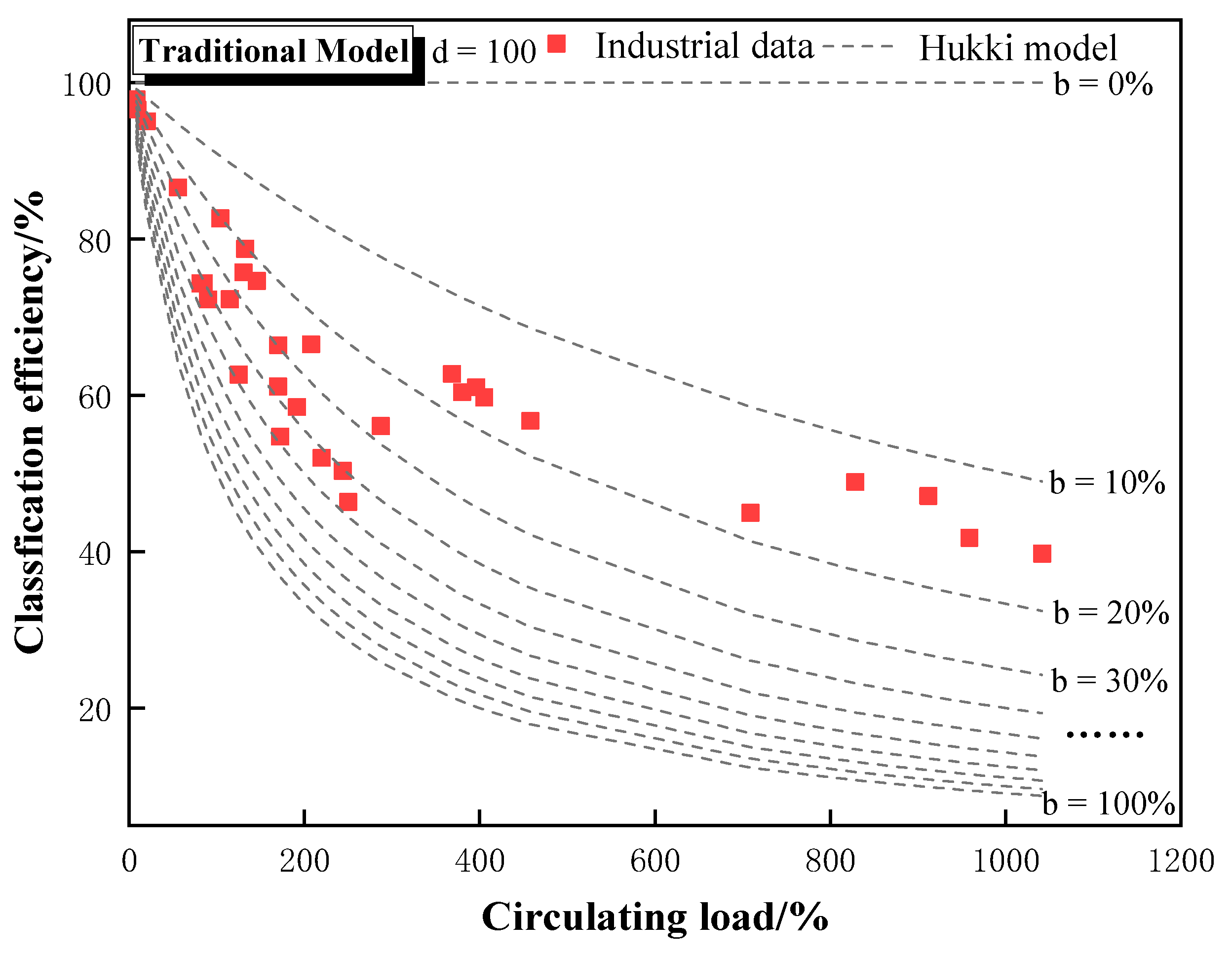
Figure 13.
The relationship between circulating load and classification efficiency in the new model.
Figure 13.
The relationship between circulating load and classification efficiency in the new model.
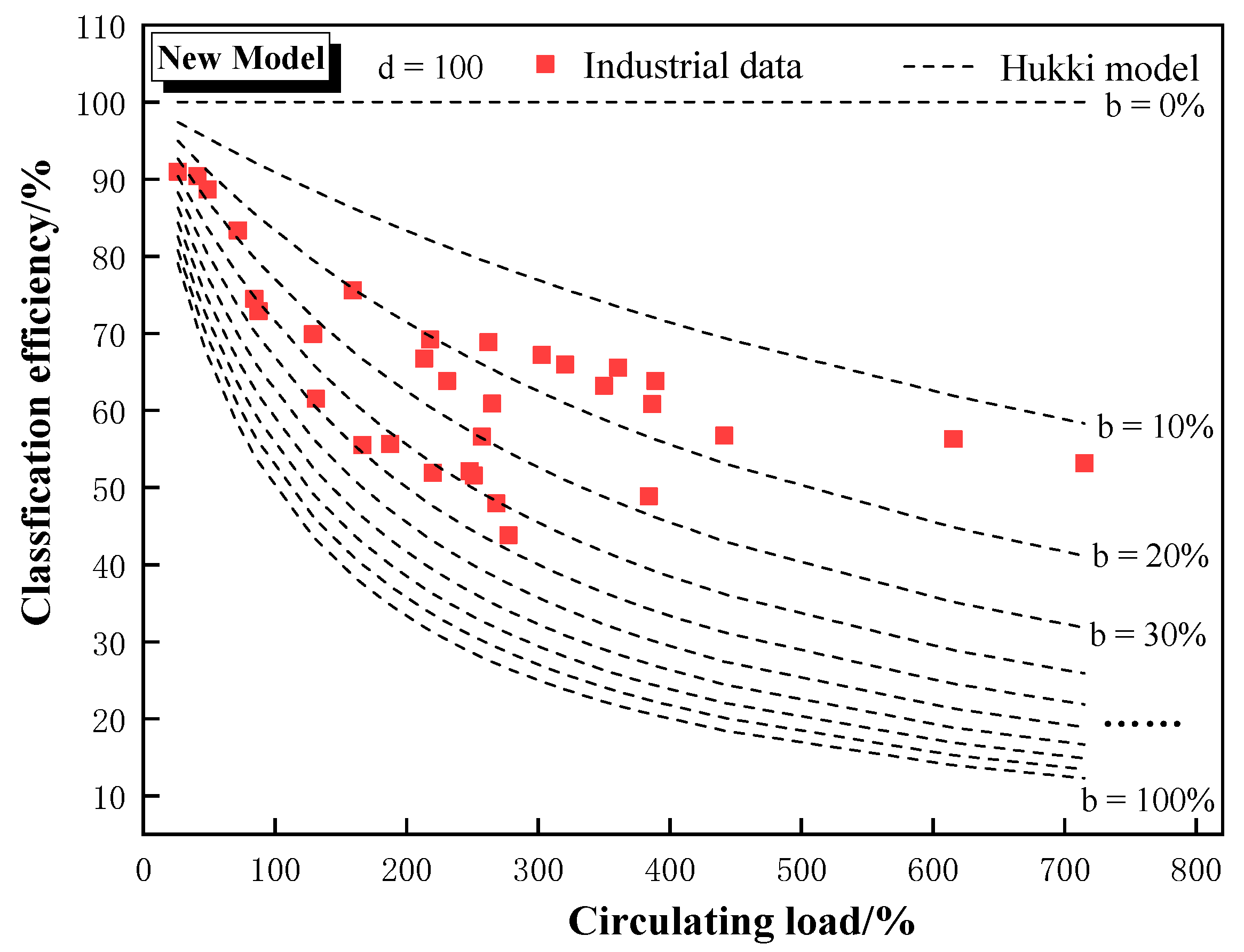

Table 1.
Main parameters of the equipment of Nanshan Mine.
| Parameters | Ball Mill | Hydrocyclone |
|---|---|---|
| type | MQY2736 | FX350 |
| Diameter/ m | 2.7 | 0.1-0.05 |
| Length/ m | 3.6 | 0.82 |
| Effective volume/ m3 | 17.66 | |
| Rotational Speed (r/min) | 20.3 | |
| Power/ kW | 430 | |
| Throughput (t/h) | 50-150 | 50-160 |
| Classification pressure (Mpa) | 0.1 |
Table 2.
Main parameters of the equipment of Longqiao Mine.
| Parameters | Ball Mill | High-frequency screen |
|---|---|---|
| type | MQY3660 | Five deck |
| Diameter/ m | 3.6 | |
| Length/ m | 6 | 2 |
| Effective volume/ m3 | 56.9 | |
| Rotational Speed (r/min) | 17.3 | |
| Power/ kW | 1250 | |
| Throughput (t/h) | 120-200 | 40 (per screen) |
| Installation angle/ ° | 22.5 | |
| Sieve hole size/ mm | 0.1 |
Table 3.
Production data and calculations for Nanshan Mine processing plant / %.
| Underflow | Overflow | Discharge | New feed | Circulating load | Classification efficiency | ||||||
|---|---|---|---|---|---|---|---|---|---|---|---|
| Traditional Model | New Model | difference | Ratio | Traditional Model | New Model | Difference | Ratio | ||||
| 12.94 | 74.97 | 25.86 | 41.10 | 380.11 | 262.15 | -117.96 | -31.03 | 60.38 | 68.85 | 8.46 | 14.02 |
| 12.94 | 74.97 | 20.61 | 41.10 | 708.74 | 441.59 | -267.14 | -37.69 | 44.98 | 56.75 | 11.77 | 26.17 |
| 9.11 | 72.26 | 15.91 | 30.41 | 828.68 | 615.44 | -213.24 | -25.73 | 48.91 | 56.31 | 7.40 | 15.14 |
| 8.92 | 61.32 | 13.51 | 43.46 | 1041.61 | 389.11 | -652.51 | -62.64 | 39.76 | 63.86 | 24.10 | 60.61 |
| 8.92 | 61.32 | 13.87 | 43.46 | 958.59 | 360.81 | -597.78 | -62.36 | 41.76 | 65.58 | 23.82 | 57.03 |
| 13.87 | 83.27 | 27.61 | 35.17 | 405.09 | 350.07 | -55.02 | -13.58 | 59.71 | 63.17 | 3.46 | 5.79 |
| 13.87 | 83.27 | 26.31 | 35.17 | 457.88 | 386.66 | -71.22 | -15.55 | 56.73 | 60.83 | 4.09 | 7.22 |
| 12.56 | 77.92 | 26.51 | 35.69 | 368.53 | 302.72 | -65.81 | -17.86 | 62.73 | 67.21 | 4.47 | 7.13 |
| 12.56 | 77.92 | 25.74 | 35.69 | 395.90 | 320.41 | -75.49 | -19.07 | 61.04 | 65.94 | 4.90 | 8.02 |
| 11.26 | 91.49 | 19.19 | 34.78 | 911.73 | 715.13 | -196.60 | -21.56 | 47.12 | 53.19 | 6.06 | 12.87 |
Table 4.
Production data and calculations for Longqiao Mine processing plant / %.
| Underflow | Overflow | Discharge | New feed | Circulating load | Classification efficiency | ||||||
|---|---|---|---|---|---|---|---|---|---|---|---|
| Traditional Model | New Model | Difference | Ratio | Traditional Model | New Model | Difference | Ratio | ||||
| 33.60 | 72.73 | 44.77 | 41.74 | 250.31 | 277.44 | 27.13 | 10.84 | 46.37 | 43.83 | -2.55 | -5.49 |
| 29.21 | 72.20 | 41.71 | 38.66 | 243.92 | 268.32 | 24.40 | 10.00 | 50.33 | 47.95 | -2.38 | -4.73 |
| 34.52 | 72.37 | 51.34 | 50.29 | 125.03 | 131.27 | 6.24 | 4.99 | 62.64 | 61.49 | -1.15 | -1.83 |
| 32.60 | 76.87 | 56.99 | 55.50 | 81.51 | 87.62 | 6.11 | 7.49 | 74.31 | 72.91 | -1.40 | -1.89 |
| 20.93 | 80.28 | 75.76 | 53.42 | 8.24 | 48.99 | 40.74 | 494.25 | 97.90 | 88.67 | -9.22 | -9.42 |
| 30.52 | 75.10 | 54.62 | 54.77 | 84.98 | 84.36 | -0.62 | -0.73 | 74.33 | 74.47 | 0.14 | 0.19 |
| 20.11 | 78.36 | 68.53 | 58.37 | 20.30 | 41.28 | 20.98 | 103.36 | 95.05 | 90.42 | -4.63 | -4.87 |
| 22.18 | 66.51 | 42.81 | 39.91 | 114.88 | 128.94 | 14.06 | 12.24 | 72.30 | 69.93 | -2.37 | -3.28 |
| 27.52 | 65.47 | 39.39 | 39.33 | 219.71 | 220.22 | 0.51 | 0.23 | 51.99 | 51.93 | -0.06 | -0.11 |
| 29.21 | 68.71 | 49.96 | 29.80 | 90.36 | 187.52 | 97.16 | 107.52 | 72.25 | 55.64 | -16.60 | -22.98 |
| 20.37 | 73.55 | 54.50 | 48.98 | 55.82 | 71.99 | 16.17 | 28.98 | 86.61 | 83.38 | -3.23 | -3.73 |
Disclaimer/Publisher’s Note: The statements, opinions and data contained in all publications are solely those of the individual author(s) and contributor(s) and not of MDPI and/or the editor(s). MDPI and/or the editor(s) disclaim responsibility for any injury to people or property resulting from any ideas, methods, instructions or products referred to in the content. |
© 2023 by the authors. Licensee MDPI, Basel, Switzerland. This article is an open access article distributed under the terms and conditions of the Creative Commons Attribution (CC BY) license (http://creativecommons.org/licenses/by/4.0/).
Copyright: This open access article is published under a Creative Commons CC BY 4.0 license, which permit the free download, distribution, and reuse, provided that the author and preprint are cited in any reuse.


