Time Reversal Symmetry Broken Floquet State of SMB_6 - A Strong Topological Insulator

1. Introduction

This communication is on a topical issue of the mixed valence compound SmB₆.[1,2,3,4,5]—a narrow gap topological Kondo insulator (TKI) which, with a high-temperature metallic phase, transforms into a paramagnetic charge insulator below 45 K. It has been suggested [6,7], as well as it is increasingly apparent [8,9,10] during the past several years, that SmB₆ is a non-trivial topological insulator. This has generated great deal of excitement in the condensed matter physics community and it still remains a matter of avid debate [6]. Despite the supporting evidence for the TKI scenario [1,2,3,4,5,6,7,8,9,10], there is no prognosis regarding the nature of the bulk and surface states of SmB₆ [11,12,13]. In this paper our primary aim is to resolve this issue. We consider an extended periodic Anderson model (EPAM) [14] for the compound SmB₆ for this purpose. We introduce here the exchange interaction (M) assuming the presence of the ferromagnetic magnetic impurities in the system. The slave boson (SB) mean-field-theoretic Anderson model of Legner [15] refers to a simple cubic lattice with one spin-degenerate orbital per lattice site each for $d\mathrm{and}f$ electrons. We consider the low-energy version of this model together with the exchange interaction. Our minimalistic Hamiltonian, based on the slave boson (SB)mean field theory of ref. [15], captures essential physics of TKI in the presence of the coulomb repulsion $U_f$ ( >> $t_{d1})$ between f electrons on the same site, and the spin-orbit hybridization V. The parameter V is the harbinger of a topological dispensation. The terms ($t_{d1},t_{f1}$) are the nearest neighbor hopping parameters for $d\mathrm{and}f$ electrons. There are three other parameters (b, λ, ξ ) of our theory [14]. While the term ξ enforces the fact that there are equal number of d and f fermions, the parameter b represents a c-number slave-boson field. We note that the constraint $U_f$>> $t_{d1}$ imposes a non-holonomic constraint, viz. the exclusion of the double occupancy. The SB-protocol provides a platform to reformulate this nonholonomic constraint into a holonomic constraint that can be implemented with the Lagrange multiplier λ. We found that λ = $-6t_{f1}+6b^2{t}_{f1},\mathrm{and}$ ξ = $-3t_{d1}+3t_{f1}$. The admissible value of $b^2$ is 1⁻. Since the method to obtain them is explained clearly in ref. [14] we will not reproduce the same here. We observe a Dirac cone like feature at $k=0$momentum in the surface state energy spectra for M = 0 [16], upon writing the SB Hamiltonian in the Dirac basis similar to the Bernevig–Hughes–Zhang (BHZ) model [17].  We obtain the Z₂ invariant (Z₂ = $-1$) using the eigenvalues of the space inversion operator in the Fu-Kane framework [18]. This is the conclusive evidence of the fact that SmB₆ is a strong topological insulator for M = 0. By calculating Berry curvature and the Chern number we have been able to show that M$\ne 0$ corresponds to the quantum anomalous Hall state. It must be mentioned here that our low-energy model has been found adequate enough to capture important features of SmB₆, although the ground state of the compound SmB₆ has been shown to be is a quartet state [1].

The exotic Floquet topological phases [19,20,21,22,23,24,25,26] with a high tunability could be realized using the circularly polarized optical field (CPOF). Analogous to the Bloch theory, here one can transform the time-dependent Hamiltonian problem to a time-independent one using the Floquet’s theorem [27,28,29,30]. The combinations of the Floquet theory with dynamical mean field theory [31], and slave boson protocol [32] were also formulated for strongly correlated systems. Our approach is in acquiescence to the latter. We use the Floquet theory[27,28,29,30,33] in section 3 in the high-frequency limit to examine the Co₃ Sn₂ S₂ thin film system. Interestingly, the incidence of CPOF leads to the time reversal symmetry (TRS) broken phase despite M = 0. The conclusive evidence of this phase being quantum spin Hall (QSH) phase is presented by calculating the spin Chern number [34,35].

The paper is organized as follows: In section 2, we calculate Z₂ invariant using the eigenvalues of the space inversion operator with in the Fu-Kane framework [18]. In section 3, we are able to show the emergence of a novel phase with broken-TRS by the normal incidence of tunable CPOF despite M = 0. For this purpose, we make use of the Floquet theory in the high-frequency limit to investigate the system. The paper ends with discussion and brief concluding remarks in section 4.

2. Surface State Hamiltonian in SB formalism and the Z₂ invariant

A. Surface State Hamiltonian

We treat the model Hamiltonian ($H_{PAM}\left(b,\mathsf{\lambda },\xi \right))$ in Eq.(1) of the ref.[14] in the low-energy limit below. All energies in our calculation/graphical representation below are expressed in units of the first neighbor hopping $t_{d_1}$ for d-electrons as this corresponds to the kinetic energy of these itinerant electrons and therefore the most dominant. In the above limit, the following replacements are necessary :$\sin \left(a_j{k}_j\right)\to a_j{k}_j+\mathrm{O}\left(a_j^3{k}_j^3\right),\cos \left(a_j{k}_j\right)\to (1-{(\frac{1}{2}a}_j^2{k}_j^2))$ where $k_j$ (j = ( x, y, z)) are momentum components, and $a_j$ is the lattice constant along j direction. Furthermore, in order to obtain surface state Hamiltonian, we make the replacement ${a{k}_z\to -ia\partial }_{\mathrm{z}}\mathrm{and}$ look for states localized within the surface z = 0 of the form $exp\left(-i\chi z\right).\mathrm{Further}\mathrm{more}$, $\mathrm{we}$ seek such a value of the unknown wave number $\chi (\chi =-iq,q>0)$ for which the exponential $exp\left(-\frac{aqz}{a}\right)\ll 1$ $\mathrm{for}z>0$. For example, if we assume $aq$ $~1$ the exponential $exp\left(-\frac{aqz}{a}\right)~\exp \left(-10\right),$ i,e vanishingly small$,\mathrm{for}z$ $~50nm$ given that SmB₆ cubic crystal structure with lattice constant a = 0.413 nm. Therefore, $\chi =-iq,q>0$ ensures a decaying term for z > 0 in the surface states. Upon including the exchange coupling M , we find that the surface state Hamiltonian $h_{\mathrm{surface}}\left(k,q,\mu ,b,M\right)$ is

$$h_{\mathrm{surface}}=\left(\begin{array}{cc}{\mathrm{Ϧ}}_{+}& {\mathcal{L}}_1\\ {\mathcal{L}}_1^{†}& {\mathrm{Ϧ}}_{-}\end{array}\right),{\mathcal{L}}_1=\left(\begin{array}{cc}0& -i{A}_{1}aq\\ -i{A}_{1}aq& 0\end{array}\right),{\mathrm{Ϧ}}_{+}=\mathrm{Ϧ}\left(k_x,k_y,q,\mu ,b,M\right)=\left(ϵ\left(k,q,\mu ,b\right)\right){\tau }_0+\mathit{n}\left(k_x,k_y,q,b\right).\mathit{\sigma }+M{\sigma }_z,{\mathrm{Ϧ}}_{-}={\mathrm{Ϧ}}^{*}\left(-k_x,-k_{y}q,\mu ,b,-M\right)$$

(1)

$\mathrm{The}\mathrm{two}\mathrm{blocks}\left({\mathrm{Ϧ}}_{+},{\mathrm{Ϧ}}_{-}\right)$,characterized by the pseudo-spin indices ( +, −), are related to each other by TRS $\mathrm{for}M=0$, and $\mathit{n}\left(k_x,k_y,q,b\right)=$ ($A_{1}a{k}_x,A_{1}a{k}_y,\vartheta \left(k_x,k_y,q,b\right)).$ The other parameters/functions in (1) are

$$A_1=2Vb,\mathit{k}=\left(k_{\mathrm{x}},k_{\mathrm{y}}\right),k^2={(k}_{\mathrm{x}}^2+k_y^2),$$

$$ϵ\left(k,q,\mu ,b\right)={ϵ}_0\left(\mu ,b\right)-D_1{(b)a}^2{q}^2+D_1(b){a^{2}k}^2+\mathrm{O}\left(a^4{q}^4\right)+\mathrm{O}\left(a^4{k}^4\right)$$

$${ϵ}_0\left(\mu ,b\right)=-\text{𝜇}+[\frac{b^2}{2}{{ϵ}_f-3t}_{d1}-3t_{f1}-6t_{d2}-6t_{f2}{b}^2-4t_{d3}-4t_{f3}{b}^2],$$

$$D_1\left(b\right)=[\frac{t_{d1}+b^2{t}_{f1}}{2}+2(t_{d2}+b^2{t}_{f2})+2(t_{d3}+b^2{t}_{f3})],$$

$$\vartheta \left(k,q,b\right)={\vartheta }_0(b){{-B_1(b)a}^{2}q}^2+B_1(b){a^{2}k}^2+\mathrm{O}\left(a^4{q}^4\right)+\mathrm{O}\left(a^4{k}^4\right),$$

$${\vartheta }_0\left(b\right)=[-\frac{b^2{ϵ}_f}{2}-6t_{d2}+6t_{f2}{b}^2-4t_{d3}+4t_{f3}{b}^2],$$

$$B_1\left(b\right)=[\frac{t_{d1}-b^2{t}_{f1}}{2}+2(t_{d2}-b^2{t}_{f2})+2(t_{d3}-b^2{t}_{f3})].$$

(2)

Here the terms $\left(t_{d1},t_{f1}\right),$ ($t_{d2},$ $t_{f2}),$ and $\left(t_{d3},t_{f3}\right),$ respectively, are the NN, NNN, and NNNN hopping parameters [14] for $d\mathrm{and}f$ electrons, ${ϵ}_f$ is the onsite energy of the $f$ electrons, μ is the chemical potential of fermion number, ${\sigma }_{x,y,z}$ are the Pauli matrices, $\mathrm{and}{\sigma }_0$ is the 2×2 identity matrix.$\mathrm{On}\mathrm{a}\mathrm{quick}\mathrm{side}\mathrm{note},$ we $\mathrm{observe}$ $\mathrm{that}{h}_{\mathrm{surface}}\left(k,q,\mu ,b,M=0\right)$ corresponds to Qi-Wu-Zhang (QWZ) model[35]. As shown by these authors, the situation corresponds to the QSH state, for the spin Hall conductance of $\mathrm{Ϧ}(\left(k_x,k_y,q,\mu ,b,M=0\right)$ and ${\mathrm{Ϧ}}^{*}\left(-k_x,-k_{y}q,\mu ,b,-M=0\right)$are not zero but the net Hall conductance of the system described by the model is zero.

For calculating the Z₂ invariant, the eigenvalues of the parity operator needs to be obtained. The objective could be accomplished with relative ease if the Hamiltonian in (1) is written down in the Dirac basis similar to the Bernevig–Hughes–Zhang (BHZ) model [17] presented over a decade and half ago for quantum wells. We now write the Hamiltonian in (1) in Dirac basis similar to the BHZ model:

$$h_{\mathrm{surface}}^{BHZ}\left(kq,\mu ,b,M\right)=\frac{{ϵ}_d+{ϵ}_c}{2}{I}^{4\times 4}+{\sum }_{a=\mathrm{0,12,3},5}{d}_a\left(k,q,\mu ,b\right){\mathsf{\gamma }}^a+M{\sigma }_0⨂{\tau }_z$$

(3)

where $d_0=\frac{{ϵ}_d-{ϵ}_c}{2}$ , ${ϵ}_d=(ϵ\left(k,q,\mu ,b\right)+\vartheta \left(k,q,b\right)),{ϵ}_c=$ $(ϵ\left(k,q,\mu ,b\right)-\vartheta \left(k,q,b\right))$, $d_1=-i{A}_{1}a{k}_y,d_2=i{A}_{1}a{k}_x,$ $d_3=A_{1}a\chi ,$ $\mathrm{and}{d}_5=0.$ The Dirac matrices (${\mathsf{\gamma }}^0,{\mathsf{\gamma }}^1,{\mathsf{\gamma }}^2,{\mathsf{\gamma }}^3,{\mathsf{\gamma }}^5)$ in con-travariant notations are ${\mathsf{\gamma }}^0=$ ${\sigma }_{}^z⨂I^{2\times 2}$ , ${{\mathsf{\gamma }}^j=i\sigma }_{}^y⨂{\tau }_{}^j,j=\mathrm{1,2},3$ , and ${\mathsf{\gamma }}^5=i{\mathsf{\gamma }}^0{\mathsf{\gamma }}^1{\mathsf{\gamma }}^2{\mathsf{\gamma }}^3$. The Pauli matrices σ and τ are acting in the space of bands that give rise to Kramers degeneracy (see Figure 1).

B. Surface state spectrum

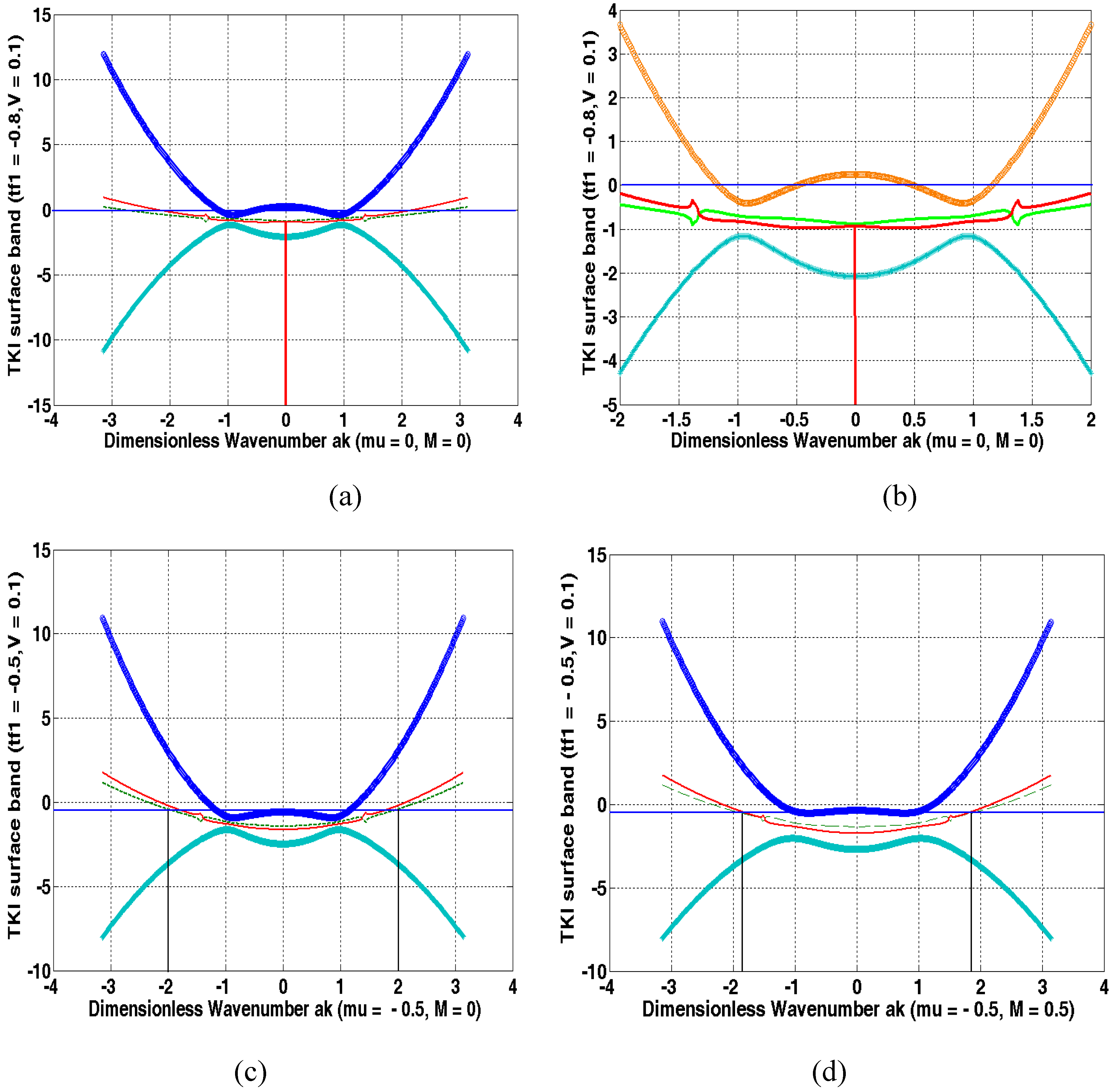
The eigenvalues ${\in }_j$ = ${\in }_j\left(s,\sigma ,k,b,M\right)$of the matrix (3) are given by a quartic and, therefore, we use Ferrari’s solution of a quartic equation (see Appendix A). We have plotted the surface state energy spectra (SSES) given by Eq. (A.2) as function of the dimensionless wave vector $ak$ in Figure 1(a) and Figure 1(b). Since the conduction bands are partially empty, the surface state will be metallic. These figures correspond to unbroken TRS (M$=0)$. It will be shown below, calculating the Z₂ invariant using the eigenvalues of the space inversion operator, that the figures correspond to QSH phase. There should be a surface Dirac cone (or at least a Kramers degeneracy) at k=0, as in ref. [16]. We indeed observe a Dirac cone like feature here (see Figure 1(a) and Figure 1(b)) in a certain parameter-window. The numerical values of the parameters used in the plots are $t_{d_1}$ = 1, $t_{f_1}$ = $-$0.8, $t_{d_2}$ = 0.01, $t_{f_2}$ = 0.01, $t_{d_3}$ = 0.001, $t_{f_3}$ = 0.001, ${ϵ}_f=$ $-$ 0.02, V = 0.1, b =0.98,μ = $0,$ ${M=0,0.3\mathrm{and}U}_f\gg t_{d_1}.$ In both the figures, $t_{f1}$ is negative and, therefore, the figures correspond to the insulating bulk. It may be noted that one needs $t_{f_1}~t_{d_1}$ to access the Dirac-cone feature. The Dirac-cone feature of SSES agrees with several experimental observations reported earlier, such as those by scanning-tunneling microscopy [36,37], angle-resolved photoemission spectroscopy (ARPES)[38,39] and the circular dichroism ARPES[40], and so on. Here, the red curve corresponds to the spin-up valence band ${\in }_3\left(s=-1,\sigma =+1,k,b\right),$and the green curve to spin-down conduction band ${\in }_2\left(s=+1,\sigma =-1,k,b\right)$. The curves display the band-inversion close to the Fermi energy represented by the horizontal solid line. In Figure 1(c), though M$=0,\mu \ne 0.$We observe that the states corresponding to momenta ak = ($\pm \mathrm{2,0})$or ( 0, $\pm 2)$ in Figure 1(a) are degenerate. Furthermore, they satisfy the condition $a\mathit{k}+a\mathit{G}=$ $-a\mathit{k}\mathrm{where}\mathrm{a}\mathit{G}\mathrm{is}\mathrm{a}\mathrm{reciprocal}$ $\mathrm{lattice}\mathrm{vector}.$ For example, for ak = ($\pm \mathrm{2,0})\mathrm{and}a\mathit{G}=\left(\mp \mathrm{4,0}\right).$ Of course, there are other possibilities too, for example ak = ( $\pm \surd 2,\pm \surd 2).$ These possibilities we are not taking into account for the simple reason that they do not satisfy the condition $\mathit{k}+\mathit{G}=-\mathit{k}.$ In Figure 1(d), M$\ne 0$ and therefore TRS is broken. There is no Kramers degeneracy as could be seen in this figure. The Figure 1(d) corresponds to QAH as is shown below.

Figure 1. The plots of surface state energy spectrum given by Equation (14) as a function of the dimensionless wave vector $ak.$ The numerical values of the parameters used in the plots are $t_{d_1}$ = 1, $t_{f_1}$ = ( $-$0.8,$-$0.5), $t_{d_2}$ = 0.01, $t_{f_2}$ = 0.01, $t_{d_3}$ = 0.001, $t_{f_3}$ = 0.001, ${ϵ}_f=$ $-$ 0.02, V = 0.1, b =0.98,μ = (0,$-0.5),$ ${M=(\mathrm{0,0.5})\mathrm{and}U}_f\gg t_{d_1}.$ The horizontal solid line represents the Fermi energy. Since the conduction bands are partially empty, the surface state will be metallic in all the cases. In (a)-(c), the system is TR symmetric. The energy bands of the system come in Kramers pairs. We observe a Dirac cone like feature in Figures (a) and (b). In Figure (d), TR symmetry is lacking and therefore no Kramers pair is possible.

Figure 1. The plots of surface state energy spectrum given by Equation (14) as a function of the dimensionless wave vector $ak.$ The numerical values of the parameters used in the plots are $t_{d_1}$ = 1, $t_{f_1}$ = ( $-$0.8,$-$0.5), $t_{d_2}$ = 0.01, $t_{f_2}$ = 0.01, $t_{d_3}$ = 0.001, $t_{f_3}$ = 0.001, ${ϵ}_f=$ $-$ 0.02, V = 0.1, b =0.98,μ = (0,$-0.5),$ ${M=(\mathrm{0,0.5})\mathrm{and}U}_f\gg t_{d_1}.$ The horizontal solid line represents the Fermi energy. Since the conduction bands are partially empty, the surface state will be metallic in all the cases. In (a)-(c), the system is TR symmetric. The energy bands of the system come in Kramers pairs. We observe a Dirac cone like feature in Figures (a) and (b). In Figure (d), TR symmetry is lacking and therefore no Kramers pair is possible.

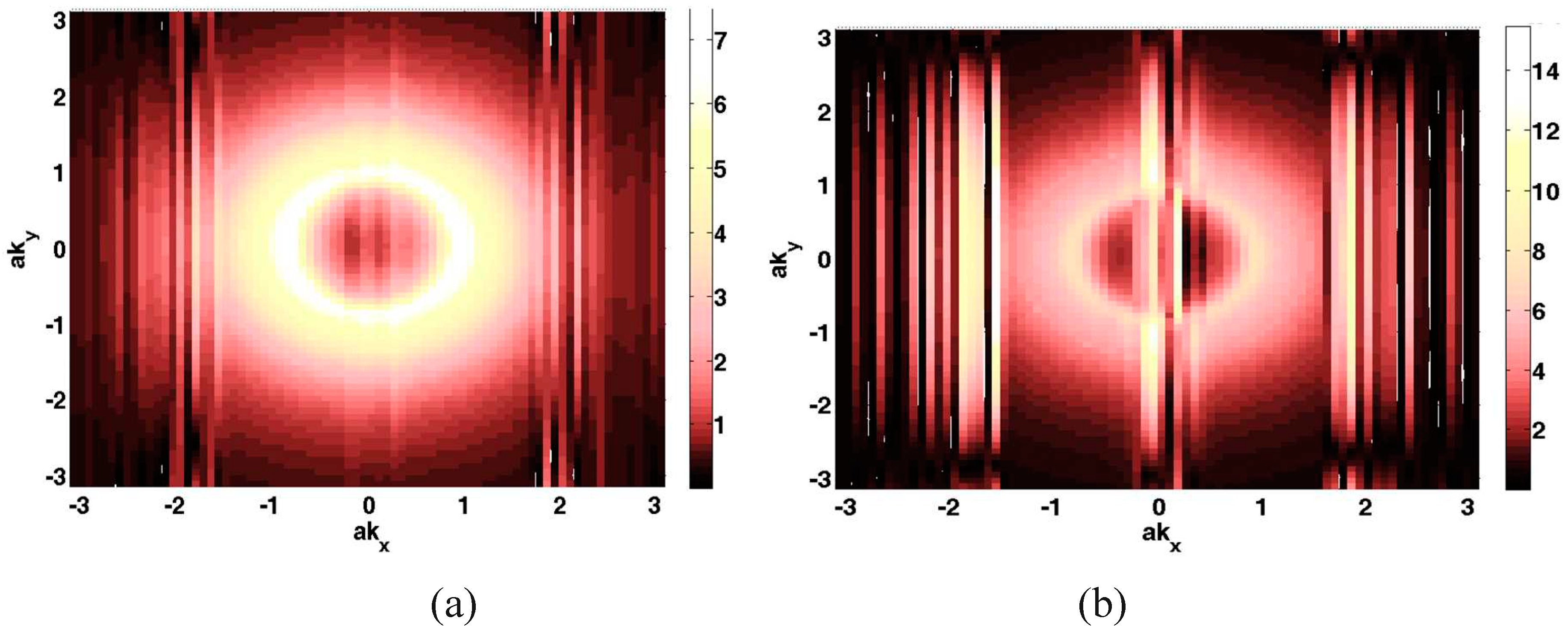
In Figure 2 we have shown the contour plots of the Berry-curvature(BC) in the z-direction for M$\ne 0.$ The numerical values of the parameters used in the plots are $t_{d_1}$ = 1, $t_{d_2}$ = 0.01, $t_{f_2}$ = 0.01, $t_{d_3}$ = 0.001, $t_{f_3}$ = 0.001, ${ϵ}_f=$ $-$ 0.02, V = 0.1, b = 0.98, μ = 0$,$ ${\mathrm{and}U}_f\gg t_{d_1}.$ The parameter $t_{f_1}$ = $-$0.8 in Figure (a) whereas $t_{f_1}$ = $-$0.6 in Figure (b). Upon integrating BC on a k-mesh-grid of the Brillouin zone (BZ), we calculate the intrinsic anomalous Hall conductivity ${\sigma }_{AH}($AHC). This yields the Chern number (C). A brief outline of the procedure followed is given below in Appendix D. We find that AHC is ${\sigma }_{AH}=$1.04$71\left(\frac{{\mathit{e}}^2}{\hslash }\right)\mathrm{in}\mathrm{the}\mathrm{formercase}(C=1.0471$ $\mathrm{is}\mathrm{close}\mathrm{to}\mathrm{the}\mathrm{integer}$ value 1), while in the latter case it is ${\sigma }_{AH}=$1.6607$(\frac{{\mathit{e}}^2}{\hslash })$. Furthermore, we found that while for $t_{f_1}=$ $-$0.4, C = 3.3906, for $t_{f_1}=$ $-$0.2, C = 3.2181. Our conjecture for not obtaining integer values of Chern number leans upon the following: The Hall conductivity ${\sigma }_{AH}$cannot be determined as such from the 2D Dirac model since Eq. (D.1) (see Appendix A) requires an integral over the whole BZ. The integral is outside the Dirac model’s range of validity. To circumvent the problem one may possibly choose a momentum space cut-off small compared to the size of BZ and large enough to capture nearly all the contributions to BC integral. This will be within the range of validity of the 2D Dirac model.

Figure 2. The contour plots of the Berry-curvature in the z-direction for M$=0.08$as a function of the dimensionless wave vector components $a{k}_x\mathrm{and}a{k}_y$. The numerical values of the parameters used in the plots are $t_{d_1}$ = 1, $t_{d_2}$ = 0.01, $t_{f_2}$ = 0.01, $t_{d_3}$ = 0.001, $t_{f_3}$ = 0.001, ${ϵ}_f=$ $-$ 0.02, V = 0.1, b =0.98, μ = 0$,$ ${\mathrm{and}U}_f\gg t_{d_1}.$ The parameter $t_{f_1}$ = $-$0.8 in Figure (a), whereas $t_{f_1}$ = $-$0.6 in Figure (b).

Figure 2. The contour plots of the Berry-curvature in the z-direction for M$=0.08$as a function of the dimensionless wave vector components $a{k}_x\mathrm{and}a{k}_y$. The numerical values of the parameters used in the plots are $t_{d_1}$ = 1, $t_{d_2}$ = 0.01, $t_{f_2}$ = 0.01, $t_{d_3}$ = 0.001, $t_{f_3}$ = 0.001, ${ϵ}_f=$ $-$ 0.02, V = 0.1, b =0.98, μ = 0$,$ ${\mathrm{and}U}_f\gg t_{d_1}.$ The parameter $t_{f_1}$ = $-$0.8 in Figure (a), whereas $t_{f_1}$ = $-$0.6 in Figure (b).

Let us now note that the Fermi energy inside the gap intersects the surface state bands in the same BZ, in general, either an even or an odd pair number of times. If there are odd numbers of pair intersections, which guarantees the time reversal invariance, the surface state is topologically non-trivial (strong topological insulator). Furthermore, it is also evident that the number of TRIM pair involved in the surface-state crossings (SSC) is one (odd). However, when there are an even number of pair-surface-state crossings, the surface states are topologically trivial (weak TI or ordinary Bloch insulators that are topologically equivalent to the filled shell atomic insulator). The quantized topological numbers, the Kane–Mele index Z₂ for QSH phase and the Chern number Ϲ for QAH phase, strongly support such topological states. The QSH band structures are characterized by the topological invariant ${\nu }_0$= 0 (Z₂= +1) and ${\nu }_0$ = 1 (Z₂ = −1). The former corresponds to weak TI, while the latter to strong TI. In fact, materials with band structures with Z₂= −1 are expected to exist in systems with strong spin-orbit coupling acting as an internal quantizing magnetic field on the electron system. The graphical representations in Figure 2 (except Figure 2(d)) indicate that the system considered here is a strong TI for M = 0. This is corroborated by analysis given below.

C. Z₂ invariant

In a bid to to calculate the Z₂ invariant using the eigenvalues of the space inversion operator, we note that the f- and d-states have different parities, the inversion symmetry(IS) operator in this band basis is constructed as Π = $I^{2\times 2}$ ⊗${\tau }_{}^z.$The time reversal (TR) operator for a spin 1/2 particle is Θ =$I^{2\times 2}⨂{\tau }^{y}K.\mathrm{The}$ operator $K\mathrm{stands}\mathrm{for}\mathrm{the}\mathrm{complex}$ conjugation. Here the${\tau }^j$ are Pauli matrices on two-dimensional spin space. The Hamiltonian under consideration, for M = 0, preserves the time reversal (TRS)and inversion symmetries (IS). It can be easily shown that $⟨\Theta \psi |\Theta \phi ⟩=⟨\phi |\psi ⟩$ taking eigenstate of the z-component of the spin operator $I^{2\times 2}⨂{\tau }^z$ as the basis. Also, Θ${\mathsf{\gamma }}^0$Θ ⁻¹ =${\mathsf{\gamma }}^0$ , Θ${\mathsf{\gamma }}^5$Θ ⁻¹ =${\mathsf{\gamma }}^5$ ,and Θ${\mathsf{\gamma }}^j$Θ ⁻¹ =$-{\mathsf{\gamma }}^j$ , where $j=\mathrm{1,2},\mathrm{and}3.$ Similarly, Π${\mathsf{\gamma }}^0$ Π ⁻¹ =${\mathsf{\gamma }}^0$ , Π${\mathsf{\gamma }}^j$ Π ⁻¹ =$-{\mathsf{\gamma }}^j$ ( $j=\mathrm{1,2})$, and Π${\mathsf{\gamma }}^k$ Π ⁻¹ =${\mathsf{\gamma }}^k$ ( $k=\mathrm{3,5}).$Since only ${\mathsf{\gamma }}^{0}and{\mathsf{\gamma }}^5$ are even under time reversal and inversion (and $d_5=0)$, at a time reversal invariant momentum(TRIM) K_i where the system preserves both TR and IS , the Hamiltonian will have the form $h_{\mathrm{surface}}^{BHZ}\left(k=K_i,q,\mu ,b,M=0\right)$ = $\frac{{ϵ}_d+{ϵ}_c}{2}{I}^{4\times 4}+d_0\left(k=K_i,q,\mu ,b\right){\mathsf{\gamma }}^0$. The eigenvalues of ${\mathsf{\gamma }}^0$are $\pm 1$( multiplicity 2). The corresponding eigenvectors are $\mid +⟩=$ (1/$\surd 2)$( 1 1 0 0)^T and $\mid -⟩=$ (1/$\surd 2)$ (0 0 $11$ )^T. Here $⟨+|{\mathsf{\gamma }}^0|+⟩=1\mathrm{and}⟨-|{\mathsf{\gamma }}^0|-⟩=-1.$ We obtain

$$⟨+|h_{\mathrm{surface}}^{BHZ}\left(k=K_i,q,\mu ,b,M=0,W_0\right)|+⟩={ϵ}_d=E_{+},⟨-|h_{\mathrm{surface}}^{BHZ}\left(k=K_i,q,\mu ,b,M=0,W_0\right)|-⟩={ϵ}_c=E_{-}.$$

(4)

Here

$$d_0=\frac{{ϵ}_d-{ϵ}_c}{2},{ϵ}_d=\left(ϵ\left(k,q,\mu ,b\right)+\vartheta \left(k,q,b\right)\right),{ϵ}_c=\left(ϵ\left(k,q,\mu ,b\right)-\vartheta \left(k,q,b\right)\right).$$

(5)

Obviously enough, if $E_{-}$ < $E_{+},$the state $\mid -⟩$ is occupied and the parity of the state at TRIM K_i is $-1.$ In the opposite case ($E_{-}$ > $E_{+})$ , the state $\mid +⟩$ is occupied and the parity is $+1.$ Therefore, the parity is given by $(-sgn\left[d_0\right]).$

We now obtain the Z₂ invariant simply by the parity eigenvalues at TRIMs. The surface states correspond to the eigenstates (or the Bloch states linked to the eigenvalues in ${\in }_j\left(s,\sigma ,k,b,M=0\right)$. These are presented in Appendix A. We consider a matrix representation of the time reversal (TR) operator Θ in the Bloch wave function basis. With α and β as the band indices we consider the representation is ${\mathsf{\xi }}_{\mathsf{\alpha }\mathsf{\beta }}\left(k\right)$ $=⟨{\mathsf{ύ}}^{\left(\alpha \right)}\left(-\mathrm{k}\right)|\mathsf{\Theta }|{\mathsf{ύ}}^{\left(\beta \right)}\left(\mathrm{k}\right)⟩$. This matrix relates the two Bloch states |${\mathsf{ύ}}^{\left(\alpha /\beta \right)}\left(-\mathrm{k}/\mathrm{k}\right)⟩\mathrm{and}$ $\mathrm{via}|{\mathsf{ύ}}^{\left(\alpha \right)}\left(-\mathrm{k}\right)⟩={\sum }_{\beta }{\mathsf{\xi }}_{\mathsf{\alpha }\mathsf{\beta }}^{*}\left(k\right)\Theta |{\mathsf{ύ}}^{\left(\beta \right)}\left(\mathrm{k}\right)⟩.$With the aid of this one can easily show that ${\mathsf{\xi }}_{\mathsf{\alpha }\mathsf{\beta }}\left(k\right)$ is a unitary matrix ( ${\mathsf{\xi }}^{†}\mathsf{\xi }=\mathrm{I})$. We also find that it has the property ${\mathsf{\xi }}_{\mathsf{\alpha }\mathsf{\beta }}\left(-k\right)$ $=-{\mathsf{\xi }}_{\mathsf{\beta }\mathsf{\alpha }}\left(k\right).$ This implies that the matrix ${\mathsf{\xi }}_{\mathsf{\alpha }\mathsf{\beta }}\left(K_i\right)$ at a TRIM becomes anti-symmetric, i.e. ${\mathsf{\xi }}_{\mathsf{\alpha }\mathsf{\beta }}\left(K_i\right)=-{\mathsf{\xi }}_{\mathsf{\beta }\mathsf{\alpha }}\left(K_i\right)$ $\ne$ 0. Only when the bands α and β form a Kramers pair, such a non-zero ${\mathsf{\xi }}_{\mathsf{\alpha }\mathsf{\beta }}$is obtained. Yet another which we need to consider is the Berry connection matrix defined as ${\gamma }_{\alpha \beta }\left(k\right)=-i⟨{\mathsf{ύ}}^{\left(\alpha \right)}\left(\mathrm{k}\right)|{\nabla }_{\mathrm{k}}|{\mathsf{ύ}}^{\left(\beta \right)}\left(\mathrm{k}\right)⟩.$ In view of the results $⟨\Theta \psi |\Theta \phi ⟩=⟨\phi |\psi ⟩$ and $|{\mathsf{ύ}}^{\left(\alpha \right)}\left(-\mathrm{k}\right)⟩={\sum }_{\beta }{\mathsf{\xi }}_{\mathsf{\alpha }\mathsf{\beta }}^{*}\left(k\right)\Theta |{\mathsf{ύ}}^{\left(\beta \right)}\left(\mathrm{k}\right)⟩$ we arrive at the relation linking ${\gamma }_{\alpha \beta }\left(k\right)$ and ${\gamma }_{\alpha \beta }\left(-k\right):$

$$\mathit{\gamma }\left(-\mathit{k}\right)\mathbf{=}\mathsf{\xi }\left(\mathit{k}\right){\mathit{\gamma }}^{\mathit{*}}\left(\mathit{k}\right){\mathsf{\xi }}^{†}\left(\mathit{k}\right)+\mathit{i}\mathsf{\xi }\left(\mathit{k}\right){\nabla }_{\mathbf{k}}{\mathsf{\xi }}^{†}\left(\mathit{k}\right).$$

(6)

Upon taking the trace we find tr$\left(\mathit{\gamma }\left(-\mathit{k}\right)\right)$= ${tr(\mathit{\gamma }}^{\mathit{*}}\left(\mathit{k}\right))+\mathit{i}tr(\mathsf{\xi }\left(\mathit{k}\right){\nabla }_{\mathbf{k}}{\mathsf{\xi }}^{†}\left(\mathit{k}\right))$. Since ${\gamma }_{\beta \alpha }={\gamma }_{\alpha \beta }^{*}$ and $\mathsf{\xi }\nabla {\mathsf{\xi }}^{†}=-(\nabla \mathsf{\xi }){\mathsf{\xi }}^{†}$, upon replacing $-\mathit{k}\mathrm{by}$ $\mathit{k}$ in the preceding equation one may write A = tr$\left(\mathit{\gamma }\left(\mathit{k}\right)\right)$= $tr(\mathit{\gamma }\left(-\mathit{k}\right))+\mathit{i}tr({\mathsf{\xi }}^{†}\left(\mathit{k}\right){\nabla }_{\mathbf{k}}\mathsf{\xi }\left(\mathit{k}\right))$.We shall need this result below. The Berry curvature of tr$\left(\mathit{\gamma }\left(\mathit{k}\right)\right)$may be defined as $\mathsf{\Omega }$ = curl A. Since the system preserves TRS and inversion symmetries (IS), one may select any gauge which renders A equal to zero. We now consider the anti-symmetric and unitary matrix ${\mathsf{\zeta }}_{\mathsf{\alpha }\mathsf{\beta }}\left(k\right)$ $=⟨{\mathsf{ύ}}^{\left(\alpha \right)}\left(\mathrm{k}\right)|\Pi \mathsf{\Theta }|{\mathsf{ύ}}^{\left(\beta \right)}\left(\mathrm{k}\right)⟩$ (where Π ² =1) to examine the consequence of setting A equal to zero. Since we find from ref.[18] that A = tr$\left(\mathit{\gamma }\left(\mathit{k}\right)\right)$ = $\frac{i}{2}tr\left({\zeta }^{†}{\nabla }_{\mathrm{k}}\zeta \right)=\frac{i}{2}{\nabla }_{\mathrm{k}}tr\left(log\zeta \right)=\mathrm{i}{\nabla }_{\mathrm{k}}\log \left(\sqrt{\det \left[\zeta \right]}\right)$), it is clear that in order to make A = 0, one needs to adjust the phase of Bloch states |${\mathsf{ύ}}^{\left(\alpha \right)}\left(\mathrm{k}\right)⟩$ such that Pf(ζ) = 1. Suppose now ρ ($K_i^{\mathrm{trim}})=\pm 1$are the eigenvalues of Π for band α at TRIM $K_i^{\mathrm{trim}},$ one obtains the matrix

$${\mathsf{\xi }}_{\mathsf{\alpha }\mathsf{\beta }}\left(K_i^{\mathrm{trim}}\right)=⟨{\mathsf{ύ}}^{\left(\alpha \right)}\left(-K_{\alpha }^{\mathrm{trim}}\right)|\Pi \Pi \mathsf{\Theta }|{\mathsf{ύ}}^{\left(\beta \right)}\left(K_i^{\mathrm{trim}}\right)⟩={\mathsf{\zeta }}_{\mathsf{\alpha }\mathsf{\beta }}\left(K_i^{\mathrm{trim}}\right){\mathsf{\rho }}_{\mathsf{\alpha }}(K_i^{\mathrm{trim}}).$$

(7)

Obviously enough, when ρ_α = ρ_β, ${\mathsf{\xi }}_{\mathsf{\alpha }\mathsf{\beta }}\left(K_i\right)=-{\mathsf{\xi }}_{\mathsf{\beta }\mathsf{\alpha }}\left(K_i\right)$ $\ne$ 0. Only when the bands α and β form a Kramers pair, such a non-zero ${\mathsf{\xi }}_{\mathsf{\alpha }\mathsf{\beta }}$ is obtained. It follows that if the bands α and β are the nth Kramers pair in the total of 2N bands, we may write ${\mathsf{\rho }}_{\mathsf{\alpha }}$= ${\mathsf{\rho }}_{\mathsf{\beta }}$ ≡ ${\mathsf{\rho }}_{2\mathrm{n}}$. From Eq.(6), one can now see that

$$Pf\left[{\mathsf{\xi }}_{\mathsf{\alpha }\mathsf{\beta }}\left(K_i^{\mathrm{trim}}\right)\right]=Pf\left[{\mathsf{\zeta }}_{\mathsf{\alpha }\mathsf{\beta }}\left(K_i^{\mathrm{trim}}\right)\right]\prod _{n=1}^N{\rho }_{2n}\left(K_i^{\mathrm{trim}}\right).$$

(8)

$\mathrm{Since}\mathrm{Pf}\left(\mathsf{\zeta }\right)=1$, in view of this result and Eq.(B.3) in the Appendix B, we find that that the Z₂ invariant can be calculated simply by the parity eigenvalues ${\rho }_{2n}$ at TRIMs $K_i^{\mathrm{trim}},$that is ${\left(-1\right)}^{\nu }=\prod _i\mathsf{\delta }\left({\mathrm{K}}_{\mathrm{trim}}^{\left(i\right)}\right)={\prod }_i\prod _n{\mathsf{\rho }}_{2\mathrm{n}}\left({\mathrm{K}}_{\mathrm{trim}}^{\left(i\right)}\right).$ Upon getting back to Eq.(5) and taking into account the observations below this equation, the parity of the occupied state at ${\mathrm{K}}_{\mathrm{trim}}^{\left(i\right)}$, viz. $\mathsf{\delta }\left({\mathrm{K}}_{\mathrm{trim}}^{\left(i\right)}\right)$ , is given by $\mathsf{\delta }\left({\mathrm{K}}_{\mathrm{trim}}^{\left(i\right)}\right)=\left(-sgn\left[d_0\right]\right).$Besides, from Eq. (4), it is easy to infer ${ϵ}_c>{ϵ}_d\mathrm{at}\mathrm{a}\mathrm{given}\mathrm{momentum}.$ This implies that $E_{-}$ > $E_{+}.$ Regarding the topology of our band system, this in turn leads to the conclusion that ν₀ = 1. Thus, indeed the system is a strong topological (non-trivial) insulator.

3. Floquet Theory

The polarized periodic optical field provides a potent modus operandi to carry out theoretical proposition and experimental realization, manipulation, and detection of diverse unconventional/novel optical and electronic properties of materials, such as the realization of novel quantum phases without static counterparts like light induced quantum anomalous phase (QAH) phase [19], the topological phase transitions in semi-metals [21,22,23,24], the Floquet engin-eering of magnetism in topological insulator thin films [41,42], and so on. The exotic Floquet topological phases with a high tunability could be realized using the polarized periodic optical field. In fact, there has been an upsurge on experimental front in the search for topological states, in solid state [42], cold-atom [43] and optical systems [44], which are driven periodically. The circularly polarized optical field (CPOF) is described by a time-periodic (time period = T = 2π/ ω where ω is the frequency of light) gauge field. Upon using the Peierls substitution, lattice electrons couple to the electromagnetic gauge field. In the presence of COPF, the thin film Hamiltonian $H_{surface,}$, apart from breaking the time reversal invariance (TRS), becomes periodic in time. One can now transform the time-dependent Hamiltonian problem to a time-independent one using the Floquet’s theorem [25,26,27,28]. Analogous to the Bloch theory, a solution for the time-dependent Schrodinger equation of the system is obtained here involving the Floquet quasi-energy and the time-periodic Floquet state with the periodicity T. The Floquet state could be expanded in a Fourier series which makes us arrive at an infinite dimensional eigenvalue equation in the Sambe space [27].The circularly polarized optical field incident upon the film may be described by a time-varying gauge field $\mathit{A}\left(t\right)=\mathit{A}\left(t+T\right)={\mathit{A}}_1\left(\mathit{sin}\left(\mathsf{\omega }\mathrm{t}\right),\mathit{sin}\left(\omega t+\psi \right),0\right)$ through the relation: $\mathit{E}\left(t\right)=-\frac{\partial \mathit{A}\left(t\right)}{\partial t}=-\mathit{E}\left(\mathit{cos}\left(\omega t\right),\mathit{cos}\left(\omega t+\psi \right),0\right)$, $\mathit{E}={\mathit{A}}_1\omega .$ Here $\mathit{E}\left(t\right)is$The optical field. In particular, when the phase ψ = 0 or π, the optical field is linearly polarized. When ψ = + π/2 ( ψ = −π/2), the optical field is left-handed ( right-handed) circularly polarized. Once we have included a gauge field, it is necessary that we make the Peierls substitution $H_{surface}\left(t\right)=H_{surface}\left(\mathbf{k}-\frac{e}{\hslash }\mathbf{A}\left(t\right)\right)$. The dimensionless quantity ${aA}_0=\frac{aeE}{\hslash \omega }$ corresponds to the frequency of the incident light.

We assume the normal incidence of CPOF on the surface SmB₆ with the thickness d = 30 nm. Suppose the angular frequency of the optical field incident on the film is ω $\approx {10}^{15}radian-s^{-1}$ and wavelength ${\lambda }_{in}\approx 1500nm.$ Therefore the ratio d/${\lambda }_{in}$ $\approx 0.02\ll 1$ Upon taking the field into consideration our Hamiltonian becomes time dependent. As stated above, the Floquet theory can be applied to our time-periodic Hamiltonian $H_{surface}\left(t\right)=H_{surface}\left(t+T\right)$ with the period $T$ = 2π/ω. Analogous to the Bloch theory involving crystal quasi-momentum, a solution | $\eta \left(t\right)⟩=\exp (-i\mathsf{έ}t)|\xi \left(t\right)⟩$ involving the Floquet quasi-energy $\mathsf{έ}$ could be written down for the time-dependent Schrodinger equation of the system. The Floquet state satisfies $\left|\xi \left(t\right)⟩=\right|\xi \left(t+T\right)⟩$ and, therefore, could be expanded in a Fourier series $|\xi \left(t\right)⟩={\sum }_r\exp \left(-ir\omega t\right)$ $|{\xi }_r⟩$ where r is an integer. Then the wave function, in terms of the quasi-energy $\mathsf{έ}$ has the form | $\eta \left(t\right)⟩$ = $\sum _r\exp \left(-i\left(\frac{\mathsf{έ}}{\hslash }+r\omega \right)\mathrm{t}\right|{\xi }_r⟩.$This makes us arrive at an infinite dimensional eigenvalue equation in the Sambe space (the extended Hilbert space)[27,28]:

$$\sum _s{H}_{surface,r,s}|{\xi }_n^s⟩=(s\hslash \mathsf{\omega }{\delta }_{r,s}+\frac{1}{T}{\int }_0^T{H}_{\mathrm{surface}}\left(t\right)e^{i\left(r-s\right)\mathsf{\omega }t}dt)\left|{\xi }_n^s⟩={\mathsf{έ}}_n\right|{\xi }_n^s⟩.$$

(9)

The matrix element of the Floquet state surface Hamiltonian $H_{surface,\alpha ,\beta }\mathrm{is}\mathrm{given}\mathrm{by}$ $H_{surface,\alpha ,\beta }=\alpha \hslash \mathsf{\omega }{\delta }_{\alpha ,\beta }+\frac{1}{T}{\int }_0^T{H}_{\mathrm{surface}}\left(t\right)e^{i\left(\alpha -\beta \right)\mathsf{\omega }t}dt,$ where ( $\alpha ,\beta$) are integers. In view of the Floquet theory [29,30,31,32], in the high-frequency limit, a thin film system, irradiated by the circularly polarized radiation, can be described by an effective, static Hamiltonian. in the off-resonant regime using the Floquet-Magnus (high-frequency) expansion [30]:

$$H_{\mathrm{surface}}^{Floquet}(k)=H_{surface,\mathrm{0,0}}+\frac{\left[H_{surface,0,-1},H_{surface,\mathrm{0,1}}\right]}{\hslash \omega }+\mathrm{O}\left({\omega }^{-2}\right),$$

(10)

where $H_{surface,n,m}=\frac{1}{T}{\int }_0^T{H}_{\mathrm{surface}}\left(t\right)e^{i\left(n-m\right)\mathsf{\omega }t}dt$ with n$\ne m.$ For M << $t_{d_1}$, we can write

$$H_{surface,\mathrm{0,0}}=h_{\mathrm{surface}}\left(k,q,\mu ,b\right)+[\frac{t_{d1}+b^2{t}_{f1}}{2}+2\left(t_{d2}+b^2{t}_{f2}\right)+2\left(t_{d3}+b^2{t}_{f3}\right)]$$

$$\times (a^2{A}_0^2){\sigma }_0⨂{\tau }_0+[\frac{t_{d1}-b^2{t}_{f1}}{2}+2(t_{d2}-b^2{t}_{f2})+2(t_{d3}-b^2{t}_{f3})](a^2{A}_0^2){\sigma }_0⨂{\tau }_z,$$

(11)

$$\begin{gathered} H_{surface,0,-1}=-\left[\frac{t_{d1}+b^2{t}_{f1}}{2}+2\left(t_{d2}+b^2{t}_{f2}\right)+2\left(t_{d3}+b^2{t}_{f3}\right)\right]i{a^2(k_x+e^{-i\psi }{k}_y)A}_0{\sigma }_0⨂{\tau }_0 \\ -[\frac{t_{d1}-b^2{t}_{f1}}{2}+2(t_{d2}-b^2{t}_{f2})+2(t_{d3}-b^2{t}_{f3})]i{a}^2{\left(k_x+e^{-i\psi }{k}_y\right)A}_0{\sigma }_0⨂{\tau }_z-(i/2)A_1(a{A}_0){\sigma }_{\mathrm{z}}\text{ ⊗}{\tau }_{\mathrm{x}}-(i/2)A_1\left(a{A}_0\right)e^{-i\psi }{\sigma }_0\otimes {\tau }_{\mathrm{y}}, \end{gathered}$$

(12)

$$\begin{gathered} H_{surface,\mathrm{0,1}}=\left[\frac{t_{d1}+b^2{t}_{f1}}{2}+2\left(t_{d2}+b^2{t}_{f2}\right)+2\left(t_{d3}+b^2{t}_{f3}\right)\right]i{a^2(k_x+e^{i\psi }{k}_y)A}_0{\sigma }_0⨂{\tau }_0 \\ +[\frac{t_{d1}-b^2{t}_{f1}}{2}+2(t_{d2}-b^2{t}_{f2})+2(t_{d3}-b^2{t}_{f3})]i{a}^2{\left(k_x+e^{-i\psi }{k}_y\right)A}_0{\sigma }_0⨂{\tau }_z \\ +(i/2)A_1{(aA}_0){\sigma }_{\mathrm{z}}\otimes {\tau }_{\mathrm{x}}+(i/2)A_1{(aA}_0)e^{i\psi }{\sigma }_0\otimes {\tau }_{\mathrm{y}}. \end{gathered}$$

(13)

From the action of the time reversal operator on the wave function we see, that it leads to a complex conjugation of the wave function. Thus, in the case of spin-less wave functions as Θ =K, where K is the operator for complex conjugation. More generally, we can write Θ = UK where U is a unitary operator. Furthermore, for a spin-1/2 particle, flipping the spin coincides with the time-reversal. This means Θ $\widehat{\mathit{S}}=-\widehat{\mathit{S}}\mathrm{where}\widehat{\mathit{S}}=\frac{1}{2}$ $\widehat{\mathsf{\sigma }}\mathrm{and}\widehat{\mathsf{\sigma }}$is the vector of Pauli matrices. In view of these, one may also choose Θ = $i{\sigma }_y⨂{\tau }_{0}K.$ Upon making use of the results Θ$\widehat{A}$Θ ⁻¹ = $\widehat{A},$ Θ$\widehat{B}$Θ ⁻¹ = $-\widehat{B},$and so on, where $\widehat{A}={\sigma }_0⨂{\tau }_0,{\sigma }_z⨂{\tau }_{y,}\dots \dots \mathrm{and}\widehat{B}={\sigma }_0⨂{\tau }_y,$……., we find that

$$\begin{gathered} \Theta H_{\mathrm{surface}}^{Floquet}\left(a{k}_x,{ak}_y\right){\Theta }^{-1} \\ =H_{\mathrm{surface}}^{Floquet}\left(-a{k}_x,{-ak}_y\right)+(4{a^{2}A}_0^{2}sin\psi /\hslash \omega )\{A_{1}a{k}_x{\sigma }_0\otimes {\tau }_{\mathrm{x}}+A_{1}a{k}_y{\sigma }_{\mathrm{z}}\otimes {\tau }_{\mathrm{y}}\}\times \left[\frac{t_{d1}+b^2{t}_{f1}}{2}+2\left(t_{d2}+b^2{t}_{f2}\right)+2\left(t_{d3}+b^2{t}_{f3}\right)\right]+\left(\frac{4a^2{A}_0^2{A}_1^{2}sin\psi }{\hslash \omega }\right){\sigma }_z\otimes {\tau }_{\mathrm{z}}, \end{gathered}$$

(14)

where Θ$H_{\mathrm{surface}}^{Floquet}\left(a{k}_x,a{k}_y\right)$Θ ⁻¹ = $H_{\mathrm{surface}}^{Floquet}\left(k\right)\left(-a{k}_x,{-ak}_y\right)$ only when $\psi =0\mathrm{or}\mathsf{\pi },\mathrm{that}\mathrm{is},$ when the optical field is linearly polarized. In this case, the time reversal symmetry (TRS) is not broken. However, when $\psi \ne 0\mathrm{or}\mathsf{\pi }$, TRS is broken. We now consider the particular cases where ψ = + π/2 and ψ = −π/2. For the former the optical field is left-handed circularly polarized, whereas for the latter it is right-handed. Thus, the (previously not known) consequence is that the incidence of the CPOF on the SmB₆ surface will be able to create a novel state with the broken TRS.

The Hamiltonian to describe this broken TRS system, in the basis ($d_{\mathrm{k},\uparrow }^{†}$ ${bc}_{\mathrm{k},\downarrow }^{†}{d}_{\mathrm{k},\downarrow }^{†}b{c}_{\mathrm{k},\uparrow }^{†})$^T, could be written as $H_{\mathrm{surface}}^{Floquet}\left(k\right)=$

$$\left(\begin{array}{cccc}{E}_1& A_{1OP}^{+}(a{k}_{-})& 0& -i{A}_{1OP}^{+}aq\\ A_{1OP}^{+}\left(a{k}_{+}\right)& E_2& -i{A}_{1OP}^{+}aq& 0\\ 0& i{A}_{1OP}^{-}aq& E_3& -A_{1OP}^{-}(a{k}_{-})\\ i{A}_{1OP}^{-}aq& 0& -A_{1OP}^{-}\left(a{k}_{+}\right)& E_4\end{array}\right)$$

(15)

where $\mathit{k}=\left(k_{\mathrm{x}},k_{\mathrm{y}}\right),$ $a{\mathrm{k}}_{\mp }=a{k}_x\mp ia{k}_y,E_1={ϵ}_{OP}+{\vartheta }_{OP}^{+},E_2={ϵ}_{OP}-{\vartheta }_{OP}^{+},{E_3=ϵ}_{OP}+{\vartheta }_{OP}^{-},E_4={ϵ}_{OP}-{\vartheta }_{OP}^{-},$ $A_{1OP}^{\pm }=A_1\left(1\pm 2B_{2}sin\psi \left(\frac{a^2{A}_0^2}{\mathrm{\hslash }\omega }\right)\right),\mathrm{and}{A}_1=2Vb$. The functions ${ϵ}_{OP}={ϵ}_{OP}\left(k,q,\mu ,b\right)$ and ${\vartheta }_{OP}^{\pm }={\vartheta }_{OP}^{\pm }\left(k,q,b\right)$ are defined below:

$${ϵ}_{OP}\left(k,q,\mu ,b\right)={ϵ}_0\left(\mu ,b\right)-D_1{\left(b\right)a}^2{q}^2+D_2\left(b\right){a^{2}k}^2+{a^{2}A}_0^2{D}_2\left(b\right)+\mathrm{O}\left(a^4{k}^4\right),$$

(16)

$${\vartheta }_{OP}^{\pm }\left(k,q,b\right)={\vartheta }_0\left(b\right){{-B_1\left(b\right)a}^{2}q}^2+B_2\left(b\right){a^{2}k}^2-\left({a^{2}A}_0^2{B}_2\pm \left(\frac{a^2{A}_0^2}{\hslash \omega }\right){sin\psi A}_1^2\right).$$

(17)

The eigenvalues (${\epsilon }_{\alpha }$) of the matrix (15) is given by the quartic ${\epsilon }_{\alpha }^4+{\gamma }_{1OP}\left(k,b\right){\epsilon }_{\alpha }^3+{\gamma }_{2OP}\left(k,b\right){\epsilon }_{\alpha }^2$ $+{\gamma }_{3OP}\left(k,b\right)$ ${\epsilon }_{\alpha }+{\gamma }_{4OP}\left(k,b\right)=0$ (α= 1,2,3,4 ) where the coefficients ${\gamma }_{\beta OP}(k,$b) (β = 1,2,3,4) are given in Appendix A (see Eqs.(A.21)—(A.23)). It may be noted that to denote these eigenvalues we have used the symbol var epsilon which is distinct from that in Eq. (A.1). Once again, in view of the Ferrari’s solution of a quartic equation, we find the roots as

$${\epsilon }_{\alpha }\left(s,\sigma ,k,b\right)=\mathrm{s}\sqrt{\frac{{\eta }_{OP}\left(k\right)}{2}}-\frac{{\gamma }_{1OP}\left(k,b\right)}{4}+l{\left(b_{OP}\left(k\right)-\left(\frac{{\eta }_{OP}\left(k\right)}{2}\right)+s{c}_{OP}\left(k\right)\sqrt{\frac{2}{{\eta }_{OP}\left(k\right)}}\right)}^{\frac{1}{2}}.$$

(18)

where α = 1,2,3,4, $s=\pm 1$ is the spin index and $l$ $=\pm 1$ is the band-index. The spin-down ($s=-1)$ conduction band ( $l$ $=+1)$ and the spin-up (down) ($s=\pm 1)$valence bands ( $l$ $=-1)$, denoted respectively by ${\epsilon }_2\left(l=+1,s=-1,k,b\right)$, ${\epsilon }_3\left(l=-1,s=+1,k,b\right),\mathrm{and}{\epsilon }_4\left(l=-1,s=-1,k,b\right)$ somewhat peculiar as will be shown below. The functions appearing in Eq. (18) are given by

$${\eta }_{OP}\left(k\right)=\frac{2b_{OP}\left(k\right)}{3}+{\left({∆}_{OP}\left(k\right)-{∆}_{0OP}\left(k\right)\right)}^{\frac{1}{3}}-{\left({∆}_{OP}\left(k\right)+{∆}_{0OP}\left(k\right)\right)}^{\frac{1}{3}},$$

(19)

$${∆}_{0OP}(k)=(\frac{b_{OP}^3\left(k\right)}{27}-\frac{b_{OP}\left(k\right)d_{OP}\left(k\right)}{3}-c_{OP}^2(k)),$$

(20)

$${∆}_{OP}\left(k\right)={(\frac{2}{729}{b}_{OP}^6+\frac{{4d_{OP}^{2}b}_{OP}^2}{27}+c_{OP}^4-\frac{{d_{OP}b}_{OP}^4}{81}-\frac{{2b}_{OP}^3}{27}+\frac{{2c_{OP}^{2}b}_{OP}{d}_{OP}}{3}+\frac{d_{OP}^3}{27})}^{1/2}$$

(21)

$$b_{OP}\left(k\right)=\left\{\frac{3{{\gamma }_{1OP}\left(k,b\right)}^2-8{\gamma }_{2OP}\left(k,b\right)}{16}\right\},c_{OP}\left(k\right)=\left\{\frac{-{{\gamma }_{1OP}\left(k,b\right)}^3+4{\gamma }_{1OP}\left(k,b\right){\gamma }_{2OP}\left(k,b\right)-8{\gamma }_{3OP}\left(k,b\right)}{32}\right\},$$

(22)

$$d_{OP}\left(k\right)=\frac{-3{{\gamma }_{1OP}\left(k,b\right)}^4+256{\gamma }_{4OP}\left(k,b\right)-64{\gamma }_{1OP}\left(k,b\right){\gamma }_{3OP}\left(k,b\right)+16{{\gamma }_{1OP}\left(k,b\right)}^2{\gamma }_{2OP}\left(k,b\right)}{256}.$$

(23)

The eigenvectors corresponding to ${\epsilon }_{\alpha }^{’}s$ could be calculated in a manner given in the Appendix A. The value of $a^2{A}_0^2\left(\mathrm{dimensionless}\mathrm{intensity}\mathrm{of}\mathrm{the}\mathrm{radiation}\right)\mathrm{is}\mathrm{taken}\mathrm{to}\mathrm{be}$ around 0.8 which is good enough for the $\mathrm{radiation}$ field of frequency $\nu ~3\times {10}^{14}Hz$under consideration. Moreover, $sin\psi$ = +1 ( $sin\psi$ = − 1 sign) corresponds to the left-handed (right-handed) circularly polarized radiation above. We notice from above that CPOF not only renormalizes d and f electron hopping integrals but also does the renormalization of the hybridization parameter(HP) $.$ We have the renormalized hybridization parameters(HP) as $A_{1OP}^{\pm }=A_1\left(1\pm 2B_{2}sin\psi \left(\frac{a^2{A}_0^2}{\hslash \omega }\right)\right),$ and $A_1=2Vb$. As $B_2\left(b\right)\approx$[ $\frac{t_{d1}-b^2{t}_{f1}}{2}]>0,\mathrm{w}$e find that the renormalized HP $A_{1OP}^{+}$ > $A_1$ ( $A_{1OP}^{+}$ < $A_1)$for the left-handed (right-handed) CPOF. However, the renormalized HP $A_{1OP}^{-}$ < $A_1$ ( $A_{1OP}^{-}$ > $A_1)$ for the left-handed(right-$\mathrm{handed})\mathrm{CPOF}.\mathrm{We}$note that, in principle, when a renor-malized parameter is less than $A_1,$ it is possible that there is a critical intensity of the radiation $a^2{A}_0^2\approx$ $\frac{\left(\hslash \omega \right)}{\left(t_{d1}-b^2{t}_{f1}\right)}$ at a given frequency at which the RHP in question will be zero. This, however, may affect the topological nature of the material. Now the nearest neighbor hopping elements $t_{d1}\mathrm{and}{t}_{f1}$are related to the band masses by $t_{d1,f1}\approx \frac{{\hslash }^2}{2m_{d,f}{a}^2}.$ If one takes for the band masses $m_d\left(m_f\right)=1.5m_e\left(50m_e\right),$ where $m_e\mathrm{is}\mathrm{the}\mathrm{rest}\mathrm{mass}\mathrm{of}\mathrm{the}\mathrm{electron},$ then the corresponding values of the hopping matrix elements are $t_{d1}$ ≈ 150 meV and $t_{f1}$≈ 4.5 meV. This yields the critical intensity of the radiation $a^2{A}_0^2\approx 2.25$ which is roughly three times the intensity value assumed in the graphical representations in Figure 3.

Figure 3. The plots of energy eigenvalues ${\epsilon }_{\alpha }\left(s,\sigma ,k,b\right)$ in Eq.(31) as a function of ak for $\mathrm{a}\mathrm{given}$ intensity of incident radiation $a{A}_0$ = (0.80, 0.50). The Figures 4(a) and 4(b), respectively, corresponds to the plots for the left handed and the right-handed CPOF. The same is true for the Figures 4(c) and 4(b). The numerical values of the parameters used in the plots in (a) and (b) are $t_{d_1}$ = 1, $t_{f_1}$ = $-$0.8, $t_{d_2}$ = 0.01, $t_{f_2}$ = 0.01, $t_{d_3}$ = 0.001, $t_{f_3}$ = 0.001, ${ϵ}_f=$ $-$ 0.02, V = 0.1, b =0.98,μ = $0,a{A}_0=0.8,{M=0.0001\approx 0,andU}_f\gg t_{d_1}.$ The numerical values corresponding to (c) and (d) are μ = $-0.5,\mathrm{and}a{A}_0=0.5$ ; the rest of the values are the same as in (a) and (b).The horizontal lines represent the Fermi energy.

Figure 3. The plots of energy eigenvalues ${\epsilon }_{\alpha }\left(s,\sigma ,k,b\right)$ in Eq.(31) as a function of ak for $\mathrm{a}\mathrm{given}$ intensity of incident radiation $a{A}_0$ = (0.80, 0.50). The Figures 4(a) and 4(b), respectively, corresponds to the plots for the left handed and the right-handed CPOF. The same is true for the Figures 4(c) and 4(b). The numerical values of the parameters used in the plots in (a) and (b) are $t_{d_1}$ = 1, $t_{f_1}$ = $-$0.8, $t_{d_2}$ = 0.01, $t_{f_2}$ = 0.01, $t_{d_3}$ = 0.001, $t_{f_3}$ = 0.001, ${ϵ}_f=$ $-$ 0.02, V = 0.1, b =0.98,μ = $0,a{A}_0=0.8,{M=0.0001\approx 0,andU}_f\gg t_{d_1}.$ The numerical values corresponding to (c) and (d) are μ = $-0.5,\mathrm{and}a{A}_0=0.5$ ; the rest of the values are the same as in (a) and (b).The horizontal lines represent the Fermi energy.

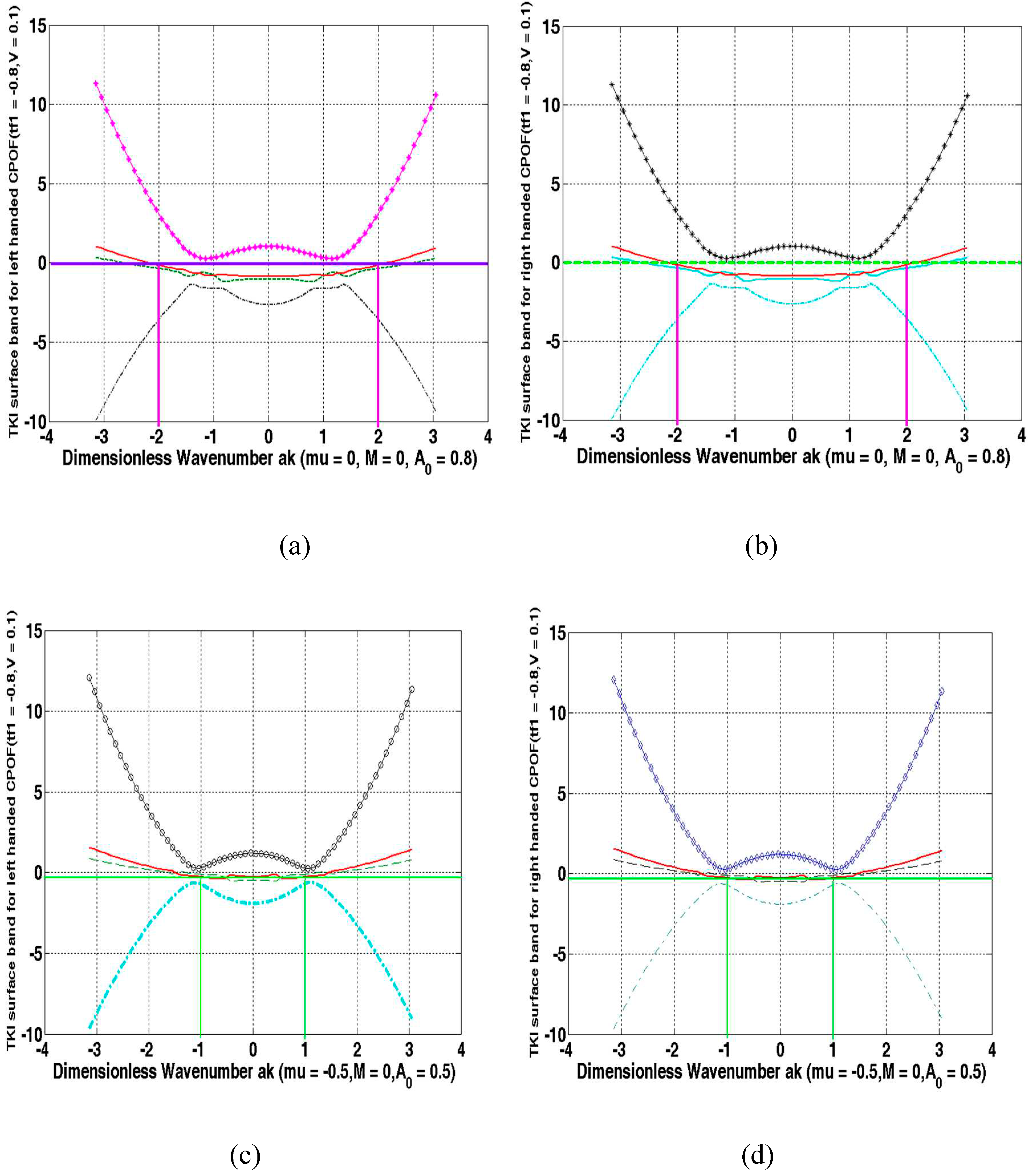
In Figure 3 (a),3(b), 3(c), and 3(d) we have plotted the energy eigenvalues ${\epsilon }_{\alpha }\left(s,\sigma ,k,b\right)$ as a function of ak for$a{A}_0$ = (0.80,0.50) for the circularly polarized light. Whereas Figures 3(a) and 3(c) correspond to left-handed CPOF, 3(b) and 3(d) to the right-handed CPOF. The numerical values of the parameters used in the plots are $t_{d_1}$ = 1, $t_{f_1}$ = $-$0.8, $t_{d_2}$ = 0.01, $t_{f_2}$ = 0.01, $t_{d_3}$ = 0.001, $t_{f_3}$ = 0.001, ${ϵ}_f=$ $-$ 0.02, V = 0.1, b =0.98,μ = ( $0,-0.5),$ ${M=0.0001\approx 0,andU}_f\gg t_{d_1}.$ The horizontal lines represent the Fermi energy. The conduction and valence bands denoted by ${\epsilon }_2\left(l=+1,s=-1,k,b\right)$, ${\epsilon }_3\left(l=-1,s=+1,k,b\right),\mathrm{and}$ ${\epsilon }_4\left(l=-1,s=-1,k,b\right)$represent-ed by differently colored curves, apart from the band-inversion, exhibit some peculiarities by way of the multiple avoided crossings and the near absence of a surface Dirac cone at k = 0 in 3(a) and 3(b) unlike that in Figure 1(a).This non-trivial feature could be ascribed to the interaction of the system with the incident radiation. The figures show that when TRS is broken despite M = 0, the fledgling novel phase of the system is very robust. The reason being in both the figures the Fermi energy intersects the band ${\epsilon }_3\left(l=-1,\mu =+1,k,b\right)$ only in the same BZ an odd pair number of times. This pair of surface state crossings (SSC)corresponds to the momenta $\mathit{k}=$ ($\pm \mathrm{2,0})$ or ($0,\pm 2)$in Figure 3(a) and Figure 3(b). However, in Figure 3(c) and Figure 3(d) the same happens at the momenta $\mathit{k}=$ ($\pm \mathrm{1,0})$ or ($0,\pm 1).$ These momenta satisfy the condition $a\mathit{k}+a\mathit{G}=-a\mathit{k},$ where the reciprocal lattice vector G is ($\mp \mathrm{4,0})$ or ($0,\mp 4)$in Figure 3(a) and Figure 3(b) and ($\mp \mathrm{2,0})$ or ($0,\mp 2)$ in Figure 3(c) and Figure 3(d). $\mathrm{O}$ur graphical representation lead to the fact that, due to the light-matter interaction, the emergent unconventional phase possibly corresponds to QSH. However, as stated in section 1, the conclusive evidence of this TRS-broken phase being QSH/QAH phase will be obtained once we calculate the spin Chern number[34] and the Z₂ invariant which are future tasks.

4. Discussion and concluding remarks

The strong correlation effects and diverse surface conditions make SmB₆ extremely complicated and almost a Gordian knot. Despite this, as we have seen above, our low-energy model was able to show that the compound is a strong TI. Our low-energy model was also able to capture the fact that there should be a surface Dirac cone at k=0(as in ref.[16]) in Figure 1(a) and 1(b) for M = 0. For M$\ne 0($Figure 1(d)), since TRS is broken, there is no Kramers degeneracy. By calculating BC and the Chern number we have been able to show that the Figure 1(d) corresponds to QAH state. In the case of the light-matter interaction in section 3, however, we need to show that the novel TRS-broken phase (despite M = 0) corresponds to QSH state. The problem needs an extensive investigation introducing an additional term

$$h_z=\left[\left(\frac{1}{2}\right)\left(-{\alpha }_{0}sin\left(k_{\mathrm{y}}a\right)\right){\sigma }_{\mathrm{x}}\otimes {(\tau }_z+{\tau }_0\right)+\left(\frac{1}{2}\right){\alpha }_{0}sin\left(k_{\mathrm{x}}a\right){\sigma }_{\mathrm{y}}\otimes {(\tau }_z+{\tau }_0)],$$

(23)

which is the Rashba spin-orbit coupling (RSOC) between the d-electrons, in Eq. (1). Here ${\mathsf{\alpha }}_0\mathrm{stands}\mathrm{for}\mathrm{the}\mathrm{strength}\mathrm{of}\mathrm{RSOC}.$ These are highlights of the present report.

The Rashba coupling can arise in the present system due to proximity of material lacking in the structural inversion symmetry. In view of the spin-polarized ARPES measurements which appear to confirm the surface helical spin texture [45,46], it would be interesting to see how does surface state react to Rashba splitting as there is evidence of for a massive surface state at the surface Brillouin zone center which can exhibit Rashba splitting[47]. The Rashba SOC is of particular importance as it is a crucial ingredient for several spintronics and topological phenomena [48].

There are many other complications to bring home the point that the system needs concerted investigations. In fact, we are presently working on three of the several issues to be discussed below in brief: (i) Since we have considered surface state quite extensively, the next step forward is an investigation on the Kondo break down[49,50]. (ii)In YbB₁₂, a finite residual temperature-linear term in the thermal conductivity κ/T(T → 0) is observed demonstrating the presence of gapless and itinerant neutral fermions [51]. On the other hand, κ/T (T → 0) in SmB₆ has been controversial [52,53]. While κ/T(T → 0) of SmB₆ has been reported to be very small but finite [54,55,56], the absence of κ /T(T → 0) has been reported in references [55,57]. It is worth mentioning that in ref.[58] κ/T(T → 0) has been shown to be finite. In view of the fact that TKI are found to be exceptionally sensitive to impurities, the issue needs to be looked into. (iii) Finally, in the quantum oscillation (QO) experiments of Li et al. [59], the signatures of two-dimensional Fermi surfaces supporting the presence of topological surface states were obtained. Various theoretical models were put forward that invoke novel itinerant low-energy neutral excitations [60] within the charge gap. These excitations were proposed to produce magneto quantum oscillation (MQO) signals. The theoretical models which entered the fray are based on magnetoexcitons [61], scalar Majorana fermions [62], emergent fractionalized quasiparticles [63] and non-Hermitian states [64]. As has been reported earlier [61], in SmB₆, the QOs are observed only in the magnetization (de Haas-van Alphen(dHvA)effect). The dHvA oscillations strongly deviate below 1 K from the Lifshitz-Kosevich theory (LKT) possibly due to the presence of magnetic impurities [65]. It must be mentioned that the QOs in YbB₁₂ [66] are observed in both magnetization (the de Haas-van Alphen, dHvA, effect) and resistivity (the Shubnikov-de Haas, SdH, effect) at applied magnetic fields H where the hybridization gap is still finite. The temperature-dependence of the oscillation amplitude complies with the expectations of Fermi-liquid theory [66]. It is hoped that the details of the problematic issues given above, related/unrelated to the present communication, will motivate the condensed matter physics community to delve deeper into this problem.

In conclusion, looking at the controversies and the possibilities, it is anybody’s guess that there are many unsettled issues. Unless other TKI candidates are discovered and thoroughly studied, it is perhaps difficult to achieve enhancement in the current understanding of strongly correlated topological insulators. In this backdrop, it is pertinent to make an attempt to investigate thoroughly what exactly are the physical explanation of the issues involved. In a future communication, as we already stated, we undertake a part of this demanding task.

References

- Amorese, O. Stockert, K. Kummer, N. B. Brookes, Dae-Jeong Kim, Z. Fisk, M. W. Haverkort, P. Thalmeier, L. Hao Tjeng, and A. Severing, Phys. Rev. B 100, 241107(R) (2019). [CrossRef]
- S. R. Panday and M. Dzero, Interacting fermions in narrow-gap semiconductors with band inversion, J. Phys.: Condens. Matter 33 275601(2021). [CrossRef]
- A. Stern, M. Dzero, V.M. Galitski, Z. Fisk and J. Xia, Surface-dominated conduction up to 240 K in the Kondo insulator SmB6 under strain, Nat. Mater. 16 708 (2017). [CrossRef]
- P. P. Baruselli and M. Vojta, Kondo holes in topological Kondo insulators: Spectral properties and surface quasiparticle interference, Phys. Rev. B 89, 205105 (2014). [CrossRef]
- L. Miao, C.-H. Min, Y. Xu, Z. Huang, E. C. Kotta, R. Basak, M. S. Song, B. Y. Kang, B. K. Cho, K. Kißner, F. Reinert, T. Yilmaz, E. Vescovo, Yi-D. Chuang, W. Wu, J. D. Denlinger, and L. A. Wray, Phys. Rev. Lett. 126, 136401 (2021).
- M. Dzero, K Sun, V. Galitski, P. Coleman, Phys. Rev. Lett. 2010, 104, 106408(2010); ibid Rev. B 2012, 85, 045130 ( 2012).
- D. J. Kim, S.Thomas.; T. Grant, J. Botimer, Z. Fisk, J.Xia, Sci. Rep., 3, 3150(2013).
- S. Wolgast, C. Kurdak, K. Sun, J. W. Allen, D.-J. Kim, and Z. Fisk, Phys. Rev. B 88, 180405 (2013).
- X. Zhang, N. P. Butch, P. Syers, S. Ziemak, R. L. Greene, and J. Paglione, Phys. Rev. X 3, 011011 (2013).
- D. J. Kim, J. Xia, and Z. Fisk, Nat. Mater. 13, 466 (2014).
- P. K. Biswas, M. Legner, G. Balakrishnan, M. C. Hatnean, M. R. Lees, D. M. Paul, E. Pomjakushina, T. Prokscha, A. Suter, T. Neupert, et al., Phys. Rev. B 95, 020410 (2017).
- A. P. Sakhya and K.B. Maiti , Scientific Reports volume 10, Article number: 1262 (2020).
- N. Wakeham, P. F. S. Rosa, Y. Q. Wang, M. Kang, Z. Fisk, F. Ronning, and J. D. Thompson, Phys. Rev. B 94, 035127 (2016).
- Udai Prakash Tyagi, Kakoli Bera and Partha Goswami, On Strong f-Electron Localization Effect in a Topological Kondo Insulator, Symmetry,13(12), 2245 (2021); https://doi.org/10.3390/sym13122245. [CrossRef]
- M. Legner, Topological Kondo insulators: materials at the interface of topology and strong correlations(Doctoral Thesis),ETH Zurich Research Collection(2016).Link:https://www.research-collection.ethz.ch/bitstream/ handle/20.500. 11850/155932/eth-49918-02.pdf?isAllowed=y&sequence=2.
- F.Lou, J.-Z. Zhao, H.Weng, and X. Dai, Phys. Rev. Lett. 110, 096401(2013).
- B. A. Bernevig, T. L. Hughes, and S.-C. Zhang: Science 314, 1757 (2006).
- L. Fu, C.L. Kane.: Time reversal polarization and a Z2 adiabatic spin pump. Phys. Rev. B 74, 195312 (2006); L. Fu, C. L. Kane, and E.J. Mele: Topological insulators in three dimensions. Phys. Rev. Lett. 98, 106803 (2007); C. L. Kane, and E.J. Mele: Z2 Topological Order and the Quantum Spin Hall Effect. Phys. Rev. Lett. 95, 146802 (2005).
- S. S. Dabiri, H. Cheraghchi, and A. Sadeghi, Light-induced topological phases in thin films of magnetically doped topological insulators Physical Review B 103, 205130 (2021); H. Xu, J. Zhou, and J. Li, Light-induced quantum anomalous Hall effect on the 2D surfaces of 3D topological insulators, Advanced Science, 2101508 (2021).
- W. Zhu, M. Umer, and J. Gong, Floquet higher-order Weyl and nexus semimetals, Phys. Rev. Research 3, L032026 (2021). [CrossRef]
- L. Zhou, C. Chen, and J. Gong, Floquet semimetal with Floquet-band holonomy, Phys. Rev. B 94, 075443 (2016). [CrossRef]
- H. Hubener, M. A. Sentef, U. D. Giovannini, A. F. Kemper, and A. Rubio, Creating stable Floquet–Weyl semimetals by laser-driving of 3D Dirac materials, Nat. Commun. 8, 13940 (2017). [CrossRef]
- D. Zhang, H. Wang, J. Ruan, G. Yao, and H. Zhang, Engineering topological phases in the Luttinger semimetal α-Sn, Phys. Rev. B 97, 195139 (2018). [CrossRef]
- H. Liu, J.-T. Sun, and S. Meng, Engineering Dirac states in graphene: Coexisting type-I and type-II Floquet-Dirac fermions, Phys. Rev. B 99, 075121 (2019). [CrossRef]
- L. Li, C. H. Lee, and J. Gong, Realistic Floquet semimetal with exotic topological linkages between arbitrarily many nodal loops, Phys. Rev. Lett. 121, 036401 (2018). [CrossRef]
- X. Liu, P. Tang, H. H¨ubener, U. De Giovannini, W. Duan, and A. Rubio, arXiv preprint arXiv:2106.06977 (2021). 22. F. Qin, R. Chen, and H.-Z. Lu, J. Phys. Condens. Matter 34, 225001 (2022).
- H. Sambe, Steady states and quasi-energies of a quantum mechanical system in an oscillating field, Phys. Rev. A 7, 2203 (1973).
- A. A. Pervishko, D. Yudin, and I. A. Shelykh, Impact of high-frequency pumping on anomalous finite-size effects in three-dimensional topological insulators, Phys. Rev. B 97, 075420 (2018). [CrossRef]
- R. Chen, B. Zhou, and D.-H. Xu, Floquet Weyl semimetals in light-irradiated type-II and hybrid line node semimetals, Phys. Rev. B 97, 155152 (2018).; R. Chen, D.-H. Xu, and B. Zhou, Floquet topological insulator phase in a Weyl semimetal thin film with disorder, Phys. Rev. B 98, 235159 (2018). [CrossRef]
- N. Goldman and J. Dalibard, Periodically Driven Quantum Systems: Effective Hamiltonians and Engineered Gauge Fields, Phys. Rev. X 4, 031027 (2014); A. Eckardt and E. Anisimovas, High-frequency approximation for periodically driven quantum systems from a Floquet-space perspective, New J. Phys. 17, 093039 (2015). [CrossRef]
- N. Tsuji, T. Oka, and H. Aoki, Correlated electron systems periodically driven out of equilibrium: Floquet+DMFT formalism, Phys. Rev. B 78, 235124 (2008). [CrossRef]
- B. H. Wu and J. C. Cao, Noise of Kondo dot with ac gate: Floquet–Green’s function and noncrossing approximation approach,Phys. Rev. B 81, 085327 (2010). [CrossRef]
- S. Kohler, J. Lehmann, and P. H¨anggi, Driven quantum transport on the nanoscale ,Phys. Rep. 406, 379 (2005). [CrossRef]
- Y. Yang, Z. Xu , L. Sheng , B. Wang, D. Y. Xing , and D. N. Sheng, Time-reversal-symmetry-broken quantum spin Hall effect, Phys. Rev. Lett. 107, 066602(2011). [CrossRef]
- X.-L. Qi, Y.-S. Wu, and S.-C. Zhang, Topological quantization of the spin hall effect in two-dimensional paramagnetic semiconductors, Phys. Rev. B 74, 085308 (2006). [CrossRef]
- 36.W. Ruan, C. Ye, M. Guo, F. Chen, X.Chen, G.-Ming Zhang, and Y. Wang, Phys. Rev. Lett. 112, 136401( 2014).
- S. Rößler, T.-Hwan Jang, D.-Jeong Kim, , and S. Wirth , Proc. Natl. Acad. Sci. U.S.A., 111 (13) 4798 (2014).
- M. Neupane, N. Alidoust, S. Y. Xu, et al., Surface electronic structure of the topological Kondo-insulator candidate correlated electron system SmB6. Nat Commun 4, 2991 (2013). [CrossRef]
- J. Jiang, S. Li, T. Zhang, et al., Observation of possible topological in-gap surface states in the Kondo insulator SmB6 by photoemission. Nat Commun 4, 3010 (2013). [CrossRef]
- N. Xu, P. Biswas, J. Dil, et al., Direct observation of the spin texture in SmB6 as evidence of the topological Kondo insulator. Nat Commun 5, 4566 (2014). [CrossRef]
- F. Qin, R. Chen, and H.-Z. Lu, J. Phys. Condens. Matter 34, 225001 (2022).
- J. W. McIver, B. Schulte, F.-U. Stein, T. Matsuyama, G. Jotzu, G. Meier, and A. Cavalleri, Light-induced anomalous hall effect in graphene, Nature Physics 16, 38 (2019). [CrossRef]
- 43.B. K. Wintersperger, C. Braun, F. N. Unal, A. Eckardt, ¨ M. D. Liberto, N. Goldman, I. Bloch, and M. Aidelsburger, Realization of an anomalous floquet topological system with ultracold atoms, Nature Physics 16, 1058 (2020). [CrossRef]
- C. S. Afzal, T. J. Zimmerling, Y. Ren, D. Perron, and V. Van, Realization of anomalous Floquet insulators in strongly coupled nanophotonic lattices, Phys. Rev. Lett. 124, 253601 (2020). [CrossRef]
- N. Xu, P.K. Biswas, J.H. Dil, R.S. Dhaka, G. Landolt, S. Muff, C.E. Matt, X. Shi, N.C. Plumb, M. Radović, E. Pomjakushina, K. Conder, A. Amato, S.V. Borisenko, R. Yu, H.-M. Weng, Z. Fang, X. Dai, J. Mesot, H. Ding, M. Shi, Nat. Commun. 5, 4566 (2014).
- S. Suga et al., J. Phys. Soc. Jpn 83, 014705 (2014).
- Hlawenka, P., Siemensmeyer, K., Weschke, E. et al. Samarium hexaboride is a trivial surface conductor. Nat Commun 9, 517 (2018). https://doi.org/10.1038/s41467-018-02908-7. [CrossRef]
- A. Manchon, H. C. Koo, J. Nitta, S. M. Frolov, and R. A. Duine, New perspectives for rashba spin–orbit coupling, Nat. Mater. 871(2015). [CrossRef]
- Paul, C. P´epin, and M. Norman, Phys. Rev. Lett. 98, 026402 (2007).
- V. Alexandrov, P. Coleman, O. Erten, Phys. Rev. Lett. 114, 177202 (2015).
- Y. Sato et al., Nat. Phys. 15, 954 (2019).
- Fuhrman, W.T., Chamorro, J.R., Alekseev, P. et al. Screened moments and extrinsic in-gap states in samarium hexaboride. Nat Commun 9, 1539 (2018). https://doi.org/10.1038/s41467-018-04007-z. [CrossRef]
- In fact, we have the literature where it is reported that the material may show a linear T-term in the specific heat which has a coefficient that varies between 2 and 25 mJ/mole/K2 , depending upon the sample preparation [7, 16, 17]. Doping with 5% of magnetic impurities can lead to an order of magnitude increase in the heat capacity [18].
- M. E. Boulanger et al., Phys. Rev. B. 97, 245141 (2018).
- Y. Xu et al., Phys. Rev. Lett. 116, 246403 (2016).
- M. Orendáč, et al. Isosbestic points in doped SmB6 as features of universality and property tuning. Phys. Rev. B 96, 115101 (2017).
- S. Sen et al., Physical Review Research 2, 033370 (2020).
- Chowdhury, D., Sodemann, I. & Sentil, T., Nat. Commn. 9, 1766 (2018).
- G. Li et al., Science, 346, 1208–1212(2014). This study is the first report of the quantum oscillations in magnetization in Kondo insulators.
- G. Baskaran, arXiv: 1507.03477 v1 (2015).
- Knolle, J. & Cooper, N. R., Phys. Rev. Lett. 118, 096604 (2017).
- Erten, O., Chang, P.-Y., Coleman, P. & Tsvelik, A. M., Phys. Rev. Lett. 119, 057603 (2017).
- Shen, H. and Fu, L., Phys. Rev. Lett. 121, 026403 (2018).
- W. T. Fuhrman and P. Nikoli´c, Magnetic impurities in Kondo insulators: An application to samarium hexaboride, Phys. Rev. B 101, 245118 (2020).
- Z. Xiang, Y. Kasahara, T. Asaba, B. Lawson, C. Insman, Lu Chen, K. Sugimoto, S. Kawaguchi, Y. Sato, G. Li, S. Yao, Y.L. Chen, F. Iga, J. Singleton, Y. Matsuda, and L. Li, Quantum oscillations of electrical resistivity in an insulator, Science 69, 65 (2018). [CrossRef]
Disclaimer/Publisher’s Note: The statements, opinions and data contained in all publications are solely those of the individual author(s) and contributor(s) and not of MDPI and/or the editor(s). MDPI and/or the editor(s) disclaim responsibility for any injury to people or property resulting from any ideas, methods, instructions or products referred to in the content. |
© 2023 by the authors. Licensee MDPI, Basel, Switzerland. This article is an open access article distributed under the terms and conditions of the Creative Commons Attribution (CC BY) license (http://creativecommons.org/licenses/by/4.0/).
Copyright: This open access article is published under a Creative Commons CC BY 4.0 license, which permit the free download, distribution, and reuse, provided that the author and preprint are cited in any reuse.