

Submitted:
08 August 2023
Posted:
09 August 2023
You are already at the latest version
Abstract
Due to the advantages of low latency, low power consumption and high flexibility of FPGA-based acceleration technology, it has been more and more widely studied and applied in the field of computer vision in recent years. An FPGA-based feature extraction and tracking accelerator for real-time visual odometry (VO) and visual simultaneous localization and mapping (V-SLAM) is proposed, which can realize the complete acceleration processing capability of the image front-end and directly output the feature point ID and coordinates to the backend. The accelerator consists of image preprocessing, pyramid processing, optical flow processing, and feature extraction and tracking modules. For the first time, it implements a hardware solution that combines features from accelerated segment test (FAST) corners with Gunnar Farneback (GF) dense optical flow, to achieve better feature tracking performance and provide more flexible technical route selection. In order to solve the scale invariance and rotation invariance lacking problem of FAST features, an efficient pyramid module with a five-layer thumbnail structure is designed and implemented. The accelerator is implemented on a modern Xilinx Zynq FPGA. The evaluation result shows that the accelerator can achieve stable tracking of features of violently shaking images, and is consistent with the results of MATLAB code running on PC. When operating at 100MHz, the accelerator can process 108 frames per second for 720P images and 48 frames per second for 1080P images. Compared to PC CPUs that consume seconds of time, the processing latency is greatly reduced to the order of milliseconds, making GF dense optical flow an efficient and practical technical solution on the edge side.
Keywords:
VIO
; V-SLAM
; FPGA
; histogram equalization
; FAST
; Pyramid processing
1. Introduction
With VO and V-SLAM technology, the carrier can achieve location, navigation, and mapping in the environment of GNSS signal occlusion and rejection. This makes VO and V-SLAM the core and key technologies in applications such as autonomous driving, robotics, unmanned aerial vehicles (UAV), and virtual reality (VR) (Floreano et al., 2015; Scaramuzza et al., 2011; Davison et al., 2002; Durrant-Whyte and Bailey, 2006). Compared with other autonomous positioning methods such as LiDAR (Light Detection and Ranging) and inertial measurement unit (IMU), the main challenge of visual-based solutions comes from computing power. Due to the need for fast, stable and reliable processing of high frame rate and high-resolution image stream data, VO and V-SLAM systems typically require high-performance computing platforms, which greatly increases equipment costs and limits the further large-scale application of the technology.
The above problems can be effectively solved by using chips or processors specially designed for complex tasks such as image processing, so to achieve the purpose of hardware acceleration (Xu et al., 2021; Gour et al., 2014; Chaikalis et al., 2008; Badu et al., 2022). At present, GPU and FPGA are two representative hardware acceleration technology routes, and both are widely used in the field of image processing. In contrast to CPUs and GPUs based on the von Neumann architecture, the function of each logic unit of an FPGA is determined when reprogrammed without instructions or shared memory for communication (Ákos et al., 2021). Therefore, for streaming computing tasks, FPGA has inherent advantages in latency and higher energy efficiency. In addition, FPGA is very flexible in use, which can change hardware algorithms and chip functions, to facilitate algorithm and function verification. Therefore, it can serve as both a product and a prototype platform for chip design. Due to the above advantages, FPGA has been increasingly widely used in the field of VO and V-SLAM technology in recent years.
A synchronized VIO system with FPGA preprocessing was proposed, which can provide acceleration capability for Harris of FAST corners (Nikolic et al., 2014). The system achieves acceleration capabilities of up to 20 FPS for video streams from two cameras, but does not support acceleration of optical flow calculations. Fang et al. (2017) designed a FPGA-based ORB feature extraction for real-time visual SLAM and implemented and evaluated on an Altera Stratix V FPGA, achieving a throughput of 67 FPS. The design is proven to be a good balance between performance and energy consumption. A VIO on chip system for micro UAV was developed on a Xilinx Kintex-7 XC7K355T FPGA, and supports both the VIO front-end and back-end (Zhang et al., 2017). The front-end operates at a clock frequency of 23 MHz to reach 20 FPS, the back-end operates at a clock frequency of 100 MHz to reach 5 FPS, and the design requires 32 to 86% of the available resources on the FPGA. Tang et al. (2018) uses a Xilinx FPGA SoC (Zynq UltraScale XCZU9EG) to implement a visual inertial SLAM based on ORB features, and have optimized the IO interface, the memory hierarchy, as well as the hardware accelerator. Navion is a real-time VIO accelerator for nano drones (Suleiman et al., 2018). The entire VIO system is the first fully integrated on a chip which is fabricated in 65 nm CMOS, and can process 752×480 stereo images from EuRoC dataset in real-time at 20 FPS (Burri et al., 2016). However, because it is specifically designed for micro-drone applications, Navion compromises on many fronts. For example, it can only support 480P images, and reduces character length and limits the number of feature points to compress memory. In addition, many of its hardware parameters are determined based on the simulation analysis of the EuRoC data set, which also limits the flexibility and university of its application to a certain extent.
In this contribution, an FPGA hardware acceleration solution for VO and V-SLAM application is proposed and implemented on a Xilinx Zynq FPGA (UltraScale+ MPSoC ZU15EG). The proposed accelerator consists of image preprocessing module, pyramid processing module, optical flow processing module and feature extraction and tracking module, which realizes the complete acceleration processing function of the image front-end and directly outputs the feature point ID and coordinates to the backend. Compared with other FPGA-based VO or V-SLAM acceleration solutions, the proposed accelerator adopts the contrast limited adaptive histogram equalization (CLAHE) algorithm with excellent performance to better improve the image preprocessing quality. For the first time, we have implemented a solution that combines FAST features with GF dense optical flow. Compared with the commonly used sparse optical flow, dense optical flow calculates the displacement of all pixels in the image and performs registration, resulting in better optical flow tracking performance. The implementation of edge-based acceleration for dense optical flow also provides a more flexible technical route for the backend – it can use FAST features and their corresponding optical flow for pose estimation, or directly use dense optical flow for estimation (known as the dense direct method). It also facilitates the creation of dense/semi-dense maps. In addition, to solve the scale invariance and rotation invariance lacking problem of FAST features, we designed and implemented a pyramid module with a five-layer thumbnail structure, and optimized its pipeline and memory read and write operations.
The test benchmark system was built, which can compare the processing the processing results of the same image stream data on the FPGA side and on PC side. The test results show that the accelerator can achieve stable tracking of features of violently shaking images, and is consistent with the processing results of the MATLAB code on the PC side, which proves the effectiveness and correctness of the proposed real-time V-SLAM accelerator. In terms of hardware consumption, the proposed hardware system consumes 36% of the LUTs, 52% of the BRAM and 19% of the DSP of the Zynq FPGA (UltraScale+ MPSoC ZU15EG). In terms of throughout, when the accelerator operates at a frequency of 100MHz, it can process 108 frames per second for 720P resolution images, and 48 frames per second for 1080P resolution images. The accelerator can operate at a maximum of 200MHz, further doubling the processing power. In terms of processing latency, for 720P resolution images, the accelerator takes about 10ms per frame to calculate (operating at 100MHz). Compared to PC CPUs that consume seconds of time, the processing latency is greatly reduced, making GF dense optical flow an efficient and practical technical solution on the edge side.
The remainder of the contribution is structured as follows. Section 2 introduces the acceleration scheme of the contribution, including the overall design, and the GF dense optical flow tracking and FAST feature extraction methods. Section 3 presents the hardware architecture, which mainly consists of image preprocessing, pyramid processing, optical flow processing, and feature extraction and tracking modules. Finally, in Section 4, the proposed accelerator is implemented, and the evaluation based on the test benchmark system is carried out and presented.
2. Acceleration Scheme
The overview of the proposed FPGA-based accelerator is firstly presented in this section, including its basic functionality and composition. On this basis, a brief introduction and review were conducted on the GF dense optical flow tracking and FAST feature method.
2.1. Overall design
The overview of the FPGA-based accelerator is shown in Figure 1. It can realize the hardware acceleration functions of image preprocessing, FAST key point extraction, pyramid optical flow calculation and feature tracking, and directly output the ID and coordinate data of features to the back-end (that is, the FPGA PS side).
Unlike the commonly used method of combining feature points and sparse optical flow, this contribution adopts a dense optical flow scheme. Compared to the sparse optical flow, the dense optical flow calculates the displacement of all pixels in the image and forming a dense optical flow field (Lucas & Kanade, 1981; Barron et al., 1994; Berthold & Brian, 1981). However, its disadvantages are obvious. Since the displacement of all pixels needs to be calculated (typically several million pixels), the calculation amount of the dense optical flow is significantly greater than the sparse optical flow, so it cannot be calculated in real-time on CPU. Compared to CPU, FPGA directly accesses data stream captured by the camera via AXI (Advanced eXtensible Interface) Bus and calculate the optical flow in a streaming way, making it more efficient and faster.
The FPGA acceleration solution based on the mixing of dense optical flow and FAST features can bring us at least the following benefits:
- The dense optical flow field can be used for pixel-level image registration, so the optical flow tracking accuracy is significantly better than that of the sparse optical flow.
- The backend can still use FAST features and their corresponding sparse optical flow for pose estimation or can directly use the dense optical flow for estimation, making it more flexible to use.
- The dense optical flow facilitates the construction of a complete map.
2.2. GF dense optical flow tracking
Optical flow refers to the displacement of target pixels in adjacent frame images caused by camera motion. Generally, sparse optical flow processing is faster and more suitable for low-end computing platforms (Engel et al., 2018). Compared to sparse optical flow, dense optical flow does not only select image features for calculation but calculates the displacement of all pixels in the image, and performs registration based on the optical flow field, so the effect is better than sparse optical flow.
This work uses the GF dense optical flow to obtain better visual front-end performance, which is also a currently supported optical flow method in OpenCV (Farnebäck, 2003; Xilinx, 2015). With the support of FPGA architecture and resources, GF optical flow can run at a high frame rate in real-time, overcoming the limitation of computational power. In this way, it can be used independently for direct SLAM, as well as in conjunction with feature points – just like sparse optical flow, making it a solution with strong engineering practicality.
The principle of GF optical flow is to approximate some neighborhood of each pixel with a polynomial expansion. In this process, each pixel in the neighborhood no longer has the same influence on the central pixel, but instead uses a two-dimensional Gaussian distribution in a polynomial function to assign different weights to different pixels. Consider a quadratic polynomial, giving us the local signal model, expressed in a local coordinate system,
where A is a symmetric matrix, b a vector and c a scalar. The coefficients are estimated from a weighted least squares fit to the pixels in the neighborhood, and the weight value is related to the pixel position in the neighborhood.
The result of polynomial expansion is that each neighborhood is approximated by a polynomial. For an image frame , consider the exact quadratic polynomial
and construct a new image frame
by a global displacement d,
Equating the coefficients in the quadratic polynomials yields
From Equations (4) to (6) we can obtain the displacement d,
Finally, like LK sparse optical flow, we further combine the multi-layer pyramid to solve the problems of GF optical flow tracking dynamics and local minimum convergence.
2.3. FAST feature extraction
In addition to GF dense optical flow, the FPGA-based accelerator also performs FAST feature extraction. Compared to other corner detection algorithms, FAST only needs to compare the size of pixel brightness, which is very convenient. Its calculation process is as follows (Rosten et al., 2006):
- Select a pixel point p in the image and denote its brightness as .
- Set a threshold T for .
- With pixel point p as the center, select 16 pixel points on a circle with a radius of 3.
- If the brightness of N consecutive points on the selected circle is greater than or less than , then the pixel point p can be considered as a feature point.
- Repeat the steps above to perform the same operation for each pixel.
Finally, after the above steps are completed, non-maximal suppression is generally used to preserve corners that respond to the maximum value within a certain area to avoid the problem of excessively concentrated corners. Together with the GF optical flow, the reserved corners are output and written to the DDR of PS side for back-end solving.
3 Hardware Architecture
Figure 2 illustrates the proposed FPGA-based feature extraction and tracking accelerator for real-time for real-time visual SLAM system. It mainly consists of image preprocessing, pyramid processing, optical flow processing, and feature extraction and tracking modules. In this section, we introduce each of these modules one by one.
3.1. Image preprocessing module
Through the MIPI interface, the FPGA accelerator receives and stores the raw image stream data and performs preprocessing. First, histogram equalization (HE) is performed to extend the dynamic range of the image grayscale values to increase the image contrast. The module adopts the CLAHE algorithm with excellent performance to better solve the problem of noise amplification during image equalization.
Unlike traditional HE and AHE methods, the slope of CLAHE associated with the gray-level assignment scheme is limited, which can be accomplished by allowing only a maximum number of pixels in each of the bins associated with local histogram (Gauch, 1992; Zuiderveld, 1994). The specific implementation steps are as follows:
-
The image is divided into 16 contextual regions of size 4×4, and its discrete PDF () can be calculated as following:where MN is the product of the number of rows M and columns N of image pixels, representing the total number of pixels in the image. is the number of pixels with a gray-level of . L is the maximum number of gray-levels in the image; corresponding to an 8-bit image, the value of L is 256.On this basis, the gray-level mapping function in the contextual regions can be obtained as following:where is the number of pixels with a gray-level of in the contextual region. Through the transformation of Equation (9), pixels with a gray-level of in the contextual region can be mapped to corresponding pixels with a gray-level of .
- For each sampled pixel in the image, find the points A, B, C and D from the center of the four relevant contextual regions adjacent to this pixel, with gray-level mappings , , and , respectively, as shown in Figure 3. Assuming that the original pixel intensity at the sample point X is , its new gray value is calculated by bilinear interpolation of the gray-level mappings that were calculated for each of the surrounding contextual regions:where and are normalized distances with respect to the pixel point A.
- Set a threshold for the maximum number of pixels in each of the bins associated with local histograms, and clip and reassign pixels that exceed the threshold to limit contrast enhancement and reduce background noise. After clipping the histogram, the pixels that were clipped are equally redistributed over the whole histogram to keep the total histogram count identical. In this contribution, the clip limit is set to 3, which means that for each bin associated with the local histogram, the maximum number of pixels allowed is 3 times the average histogram contents.
Then, the image is filter, which is called Gaussian blur processing. Gaussian blur can reduce image noise, reduce the level of detail, and enhance the image effect under scales, which is conducive to the down sampling of subsequent pyramid image. A Gaussian convolution kernel with a size of 7×7 and a standard deviation of σ=5 is used to perform sliding window filtering on the image. Since FPGA is not good at floating-point arithmetic, it needs to be fixed-pointed. First, the decimal portion of the Gaussian filter parameters is determined to be 12 bits. Then, enlarge the filter parameters 212=4096 times by displacement and left shift them 12 bits to retain the integer parts.
3.2. Pyramid processing module
The pyramid processing module receives images from the preprocessing module, zooms out the images four times with a sampling ratio of 2:1, resulting in a total of 5 layers of pyramid thumbnails, including the original resolution image. Afterwards, the pyramid thumbnails are synchronously output and written to the programmable logic (PL) side double date rate (DDR) synchronous dynamic random access memory (SDRAM) through the AXI interface, as shown in Figure 4.
In the PL side DDR, four consecutive frames of images (including the pyramid thumbnails) and their optical flow data are needed. This is because the FPGA receives the k st image and performs pyramid reduction, and calculates the optical flow after receiving the k+1 st image, and the optical flow calculation is carried out layer by layer along the pyramid image from top to bottom, so the processing time required is.
It can be seen from Equation (11) that the optical flow calculation from the k+1 st image continues until the k+2 st image. Similarly, the pyramid optical flow processing of the image received from frame k+1 will end at frame k+3. The memory and time usage during the entire pyramid optical flow processing are detailed in Table 1. It is worth nothing that unlike original images and their pyramid thumbnails, the portion of memory responsible for storing optical flow data only refreshes and stores the optical flow of the previous layer of thumbnails, thereby saving memory size.
3.3. Optical flow processing module
As can be seen from the last row in Table 1, there are at most two optical flow calculation threads simultaneously in each frame. For this reason, two specialized processing units (SPU) are designed and used in the optical flow processing module. In addition, the module includes a task assignment unit (TAU) and a gating unit (GU) for optical flow outputs, as shown in Figure 5.
The TAU is responsible for obtaining the status of the two SPUs and finding out which one is idle. Once the external notification signal is received (see Figure 4), the TAU sends a start signal with the group address serial number to the idle SPU.
The detailed structure of CU is shown in Figure 6. The finite state machine (FSM) calculates all addresses based on the group address serial number, and then sequentially starts state processing for the 5-layer pyramid thumbnail. The state processing of each layer includes sending memory read commands and waiting for the optical flow calculation to complete. After the state processing of a layer is completed, the FSM switches to the next layer state.
The memory read module simultaneously reads three channels of data from the PL side DDR: the previous frame image, the current frame image, and the previous layer of optical flow data. The zoom module receives the previous layer of optical flow data and zooms in it two times to output. The zoom in operation adopts bilinear interpolation method, which executes the horizontal direction first, and then the vertical direction. The GF calculation module receives the previous and current frame images, as well as optical data from the zoom module, for GF dense optical flow calculation. The GF optical flow is written into the PL side DDR through the memory write module for the optical flow calculation of the next frame image, and is also directly output to the feature extraction and tracking module.
For the two optical flow output pipelines SPU 1 and SPU 2, only one will be valid at the same time. Therefore, the GU distinguishes the output line through the valid signal and outputs the GF optical flow calculation result.
3.4. Feature extraction and tracking module
The feature extraction and tracking module is responsible for extracting and recording FAST features, and calculating their coordinates in the new image according to the optical flow results. Moreover, writes the reorganized feature point array into the PS side DDR and sends interrupt signal to the PS side after completion.
The composition of the feature extraction and tracking module is shown in Figure 7, including of feature extraction, feature saving, feature tracking, feature merging, and feature sending submodules. First, the module receives the CLAHE processed image and performs FAST feature extraction. Secondly, the feature saving submodule receives the FAST feature data of stream type through the AXI interface, and reads each item of the stream data by line buffer. If a value other than 0 is read in the line buffer, it indicates that the corresponding point in the image is a valid feature, and the image coordinates of the feature are saved in the array pointer “prevList”, as shown in Figure 8. Due to the need for ping-pong read-write operations, “prevList” needs to be neutralized in BRAM by two copies, defined as “prevList 1” and “prevList 2”, respectively.
The feature tracking submodule receives the stream type GF optical flow data through the AXI interface and converts it into mat format. Defines an array pointer “flist” to store the abbreviated coordinates of FAST features updated by optical flow tracking. Similarly, due to the need for ping-pong read-write operations, “flist” needs to be neutralized by 2 copies, defined as “flist 1” and “flist 2”, respectively. As shown in Figure 9, the left array pointer “flist 1” stores the coordinates corresponding to features of the previous frame of the image; In the middle is the full-frame optical flow data currently being output pixel by pixel, which is read by line buffer. Since the position of features in the previous frame of the image is known, the specific positions of features in the optical flow can be determined in advance.
When the full-frame optical flow data is output to these positions, the feature merging submodules reads the feature coordinates from “prevList”, uses the optical flow to track features, obtains the position of features in the next image, and stores the updated feature coordinates in the array pointer “flist 2” on the right. Finally, the feature sending submodule sends the feature ID and coordinate data from “flist 2” to the DDR, and generates an interrupt signal after completion.
4. Evaluation and Discussion
The proposed accelerator is implemented on a Xilinx Zynq FPGA in this section. Further, in order to verify the feasibility and performance of the proposed solution, a test benchmark system is built and the evaluation work is carried out.
4.1. Test benchmark system
The proposed feature extraction and tracking accelerator is implemented on a modern Xilinx Zynq FPGA (UltraScale+ MPSoC ZU15EG), a device that combines abundant hardware resources on a single chip. Hardware programmability allows a direct, lowest-level interface to the CMOS sensor, enabling a convenient and reliable image acquisition process. Moreover, to verify the feasibility and performance of the accelerator, a test benchmark system is built. It consists of the FPGA accelerator, as well as a PC. Compared with the official version, the FPGA accelerator in the test benchmark system has been slightly modified in terms of command reception and memory storage to enable comparison and verification with the PC.
The overall workflow of the test benchmark system is shown in Figure 10. It mainly includes the following operations:
- FPGA side: Receiver the MIPI image, perform the GF optical flow calculation and the FAST feature extraction and tracking processing.
- FPGA side: Store the FAST feature tracking result and original image data in the PS side DDR, and transfer them to an SD card.
- PC side: Read the raw image data from the SD card, and obtain intermediate results on image preprocessing and FAST feature extraction through high-level synthesis (HLS) simulation (Xilinx, 2014).
- PC side: Input the intermediate results to the MATLAB-based optical flow calculation and feature tracking program, to obtain the FAST feature tracking results of MATLAB.
- Compare feature tracking results from FPGA and MATLAB for verification and analysis.
4.2. Evaluation results
The proposed accelerator is implemented on a Xilinx Zynq FPGA (UltraScale+ MPSoC ZU15EG). The camera was shaken vigorously to continuously acquire images, and the test benchmark system was used to analyze and evaluate the processing results of the accelerator. The operation results show that the accelerator can stably track features of severely shaking images, and the processing results are consistent with those of MATLAB on the PC end. Figure 11 presents the dense optical flow calculation and FAST feature tracking results for one of these frames. In can be seen that the FPGA accelerator is the same as the processing results of the MATLAB benchmark, which proves the effectiveness and correctness of the proposed real-time V-SLAM accelerator.
The proposed accelerator consumes 123300 LUTs (look up table), 386.5 M bytes of BRAMs, 68 M bytes of URAMs and 686 DSPs. The specific hardware consumption and occupation are detailed in Table 2. For 720P resolution images (1280×720), it can process 100/(1280×720)=108 frames of images per second; for 1080P resolution images (1920×1080), it can process 100/(1920×10800)=48 frames of images per second. The accelerator can operate up to more than 200MHz, further doubling the processing power.
We compared the proposed hardware with the PC-based AMD multi-core CPU. Both are based on 1280×720 resolution image for dense optical flow calculation and FAST feature extraction and tracking, for the proposed hardware (operating at 100MHz), each frame takes (1280×720)/100 MHz≈10 ms; for MATLAB code running on the Ryzen R7 6800H clocked at 3.5 GHz, each frame takes about 17 s.
5. Conclusion
An FPGA-based feature extraction and tracking accelerator for real-time VIO and Visual SLAM application is presented, which can realize the complete acceleration processing function of the image front-end and directly output the feature point ID and coordinates to the backend. The accelerator performs CLAHE and Gaussian blur for image preprocessing. For the first time, it implements a solution that combines FAST features with GF dense optical flow, to achieve better feature tracking performance and provide more flexible technical route selection for the backend. In order to solve the scale invariance and rotation invariance lacking problem of FAST features, a pyramid module with a five-layer thumbnail structure is designed and implemented, and the pipeline and memory read and write operations is optimized.
The proposed accelerator is implemented on a Xilinx Zynq FPGA (UltraScale+ MPSoC ZU15EG). The evaluation results based on the test benchmark system shows that the accelerator can achieve stable tracking of features of violently shaking images, and is consistent with the processing results of the MATLAB code on the PC side. It consumes 36% of the LUTs, 52% of the BRAM and 19% of the DSP of the Zynq FPGA. When operating at 100MHz, the accelerator can process 108 frames per second for 720P images and 48 frames per second for 1080P images. Compared to PC CPUs that consume seconds of time, the processing latency is greatly reduced to the order of milliseconds, making GF dense optical flow an efficient and practical technical solution on the edge side.
Author Contributions
Conceptualization, S.X. and C.L.; methodology, C.L. and Y.G.; software, J.Z. and W.X.; validation, C.L., S.C. and F.H.; formal analysis, F.H.; investigation, J.Z. and C.L.; resources, S.X. and Y.G.; data curation, W. X. and F.H.; writing—original draft preparation, J.Z. and C.L.; writing—review and editing, J.Z. and S.X.; visualization, C.L.; supervision, C.L.; project administration, C.L.; funding acquisition, J.Z. and C.L. All authors have read and agreed to the published version of the manuscript.
Funding
This research was funded by the National Natural Science Foundation of China, grant numbers: 12273074 and 42074044.
Data Availability Statement
The data that support the findings of this study are available on request from the corresponding author upon reasonable request.
Conflicts of Interest
The funders had no role in the design of the study; in the collection, analyses, or interpretation of data; in the writing of the manuscript; or in the decision to publish the results.
References
- Ákos, M. , Jeney, M., Dominik, R., Stefan, O. (2021). Hardware accelerated image processing on FPGA based PYNQ-Z2 board. Carpathian Journal of Electronic and Computer Engineering, 14(1): 20-23. [CrossRef]
- Badu, P. , Parthasarathy, E. (2022). Hardware acceleration for object detection using YOLOv4 algorithm on Xilinx Zynq platform. J Real-Time Image Proc 19, 931–940. J Real-Time Image Proc 19, 931–940. [CrossRef]
- Burri, M. , Nikolic, J., Gohl, P., Schneider, T., Rehder, J., Omari, S., Achtelik, W.M., Siegwart, R. (2016). The EuRoC micro aerial vehicle datasets. The International Journal of Robotics Research, 35(10): 1157-1163. [CrossRef]
- Barron, J.L., Fleet, D.J., Beauchemin, S.S. (1994). Performance of optical flow techniques. International Journal of Computer Vision, 12, 43-77. [CrossRef]
- Berthold, K.P. , Brian, G.S. (1981). Determining optical flow. Artificial Intelligence, 17(1-3): 185-203. [CrossRef]
- Chaikalis, D., Passalis, G., Passalis, N., Maroulis, D., Maroulis, T. (2008). Hardware Acceleration for 3D Image Reconstruction. 2008 Panhellenic Conference on Informatics, 147-151. [CrossRef]
- Davison, A.J. & Murray, D. (2022). Simultaneous location and map-building using active vision. IEEE Transactions on Pattern Analysis and Machine Intelligence, 24(7): 865-880. [CrossRef]
- Durrant-Whyte, H.F. , & Bailey, T. (2006). Simultaneous localization and mapping: part I. IEEE Robotics & Automation Magazine, 13, 99-110. https://10.1109/MRA.2006.1638022.
- Engel, J. , Koltun, V., Cremers, D. (2018). Direct Sparse Odometry. IEEE Transactions on Pattern Analysis and Machine Intelligence, 40(3): 611-625. [CrossRef]
- Fang, W. , Zhang, Y., Yu, Bo., Liu, S. (2017). FPGA-based ORB feature extraction for real-time visual SLAM. 2017 International Conference on Field Programmable Technology (ICFPT), 275-278. [CrossRef]
- Farnebäck, G. (2003). Two-frame motion estimation based on polynomial expansion. Proceeding of the 13th Scandinavian conference on image analysis, 363-370. [CrossRef]
- Floreano, D. , Wood R.J. (2015). Science, technology and the future of small autonomous drones. Nature, 521(7553): 460-6. [CrossRef]
- Gauch, J.M. (1992). Investigations of image contrast space defined by variations on histogram equalization. CVGIP: Graphical Models and Image Processing, 54(4): 269-280. [CrossRef]
- Gour, P. N. , Narumanchi, S., Saurav, S., Singh, S. (2014). Hardware accelerator for real-time image resizing. 18th International Symposium on VLSI Design and Test, Coimbatore, 1-6. [CrossRef]
- Lucas, B.D. , & Kanade, T. (1981). An iterative image registration technique with an application to stereo vision. Proceedings of the 7th international joint conference on Artificial intelligence - Volume 2 (IJCAI), 674-679. https://dl.acm.org/doi/10.5555/1623264.1623280.
- Nikolic, J. , Rehder, J., Burri, M., Gohl, P., Leutenegger, S., Furgale, P.T., Siegwart, R. (2014). A synchronized visual-inertial sensor system with FPGA pre-processing for accurate real-time SLAM. 2014 IEEE International Conference on Robotics and Automation (ICRA), 431-437. [CrossRef]
- Rosten, E. , & Drummond, T. (2006). Machine learning for high-speed corner detection. Proceedings of the 9th European conference on Computer Vision (ECCV) - Volume Part I, 430-443. [CrossRef]
- Suleiman, A. , Zhang, Z., Carlone, L., Karaman, S., Sze, V. (2019). Navion: A 2mW Fully Integrated Real-Time Visual-Inertial Odometry Accelerator for Autonomous Navigation of Nano Drones. IEEE Journal of Solid-State Circuits, 54(4): 1106-1119. [CrossRef]
- Scaramuzza, D. , & Fraundorfer, F. (2011). Visual odometry: part I – the first 30 years and fundamentals. IEEE Robotics & automation magazine, 18(4): 80-92. [CrossRef]
- Tang, J. , Liu, S., Zhang, Z., Fang W., Zhang Y. (2018). π-SoC: Heterogeneous SoC Architecture for Visual Inertial SLAM Applications. 2018 IEEE/RSJ International Conference on Intelligent Robots and Systems (IROS), 8302-8307. [CrossRef]
- Xu, K. , Wang, X., Liu, X., Cao, C., Li, H., Peng, H., Wang, D. (2021). A dedicated hardware accelerator for real-time acceleration of YOLOv2. J Real-Time Image Proc, 18, 481-492. [CrossRef]
- Xilinx Inc. (2015). Accelerating OpenCV applications with Zynq-7000 All Programmable SoC using Vivado HLS videolibraries. [Online]. Available: https://www.xilinx.com/support/documentation/application_notes/xapp1167.pdf.
- Xilinx Inc. (2014). Vivado Design Suite tutorial high level synthesis, UG871 (v2014.1). [Online]. Available: https://www.xilinx.com/support/documentation/sw_manuals/xilinx2019_1/ug871-vivado-high-level-synthesis-tutorial.pdf.
- Zuiderveld, K. (1994). Contrast limited adaptive histogram equalization. Graphics Gems, 474-485. [CrossRef]
- Zhang, Z. , Suleiman, A., Carlone, L., Sze, V., Karaman, S. (2017). Visual-inertial odometry on chip: an algorithm-and-hardware co-design approach. Robotics: Science and Systems. [CrossRef]
Figure 1.
Overview of the acceleration function.

Figure 2.
Hardware architecture of the FPGA-based accelerator for real-time visual SLAM.
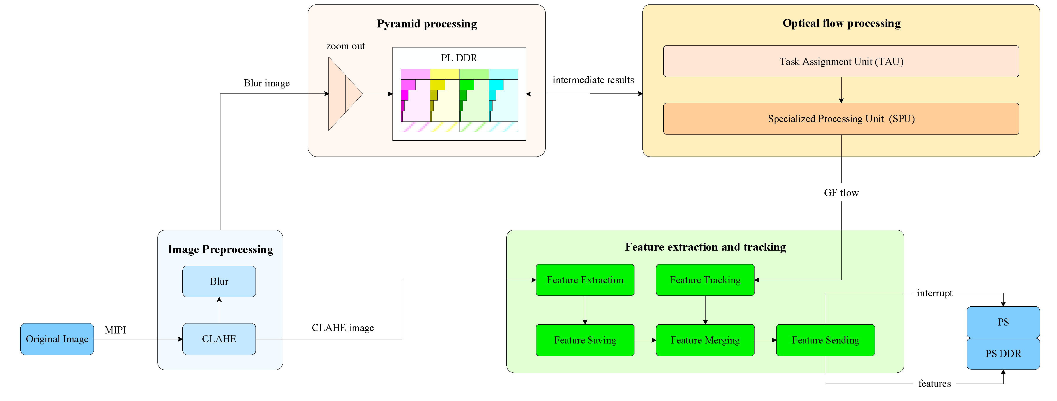
Figure 3.
Subdivision and interpolation scheme of CLAHE
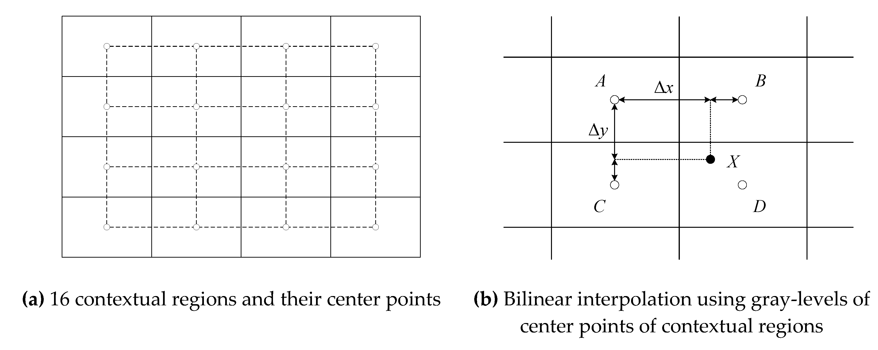
Figure 4.
Architecture of the pyramid processing module.
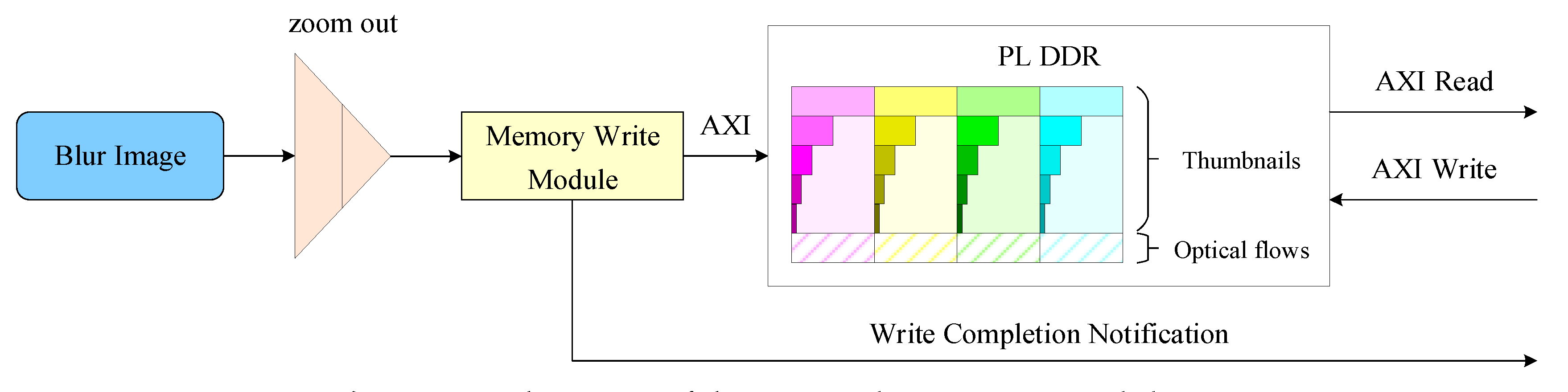
Figure 5.
Composition of the optical flow processing module
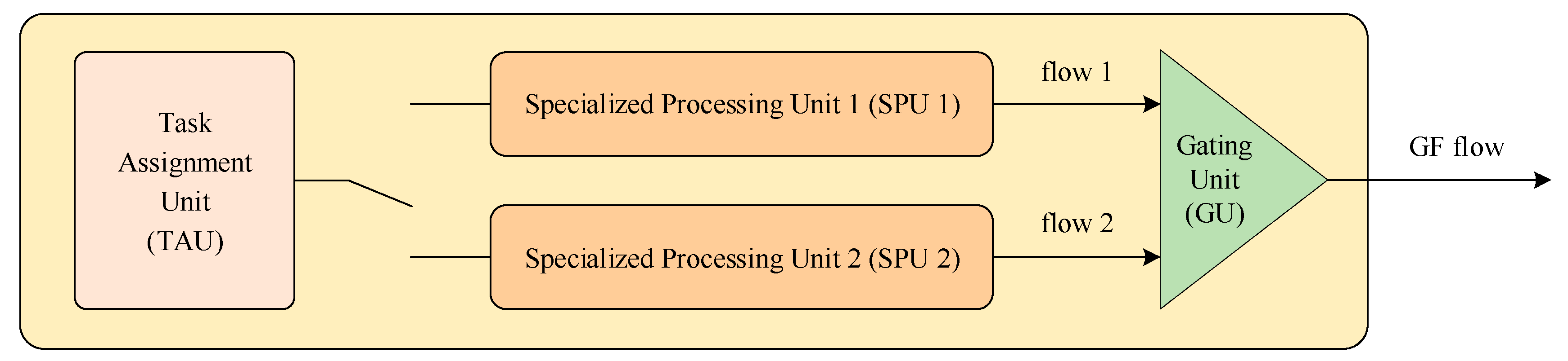
Figure 6.
Detailed structure of SPU
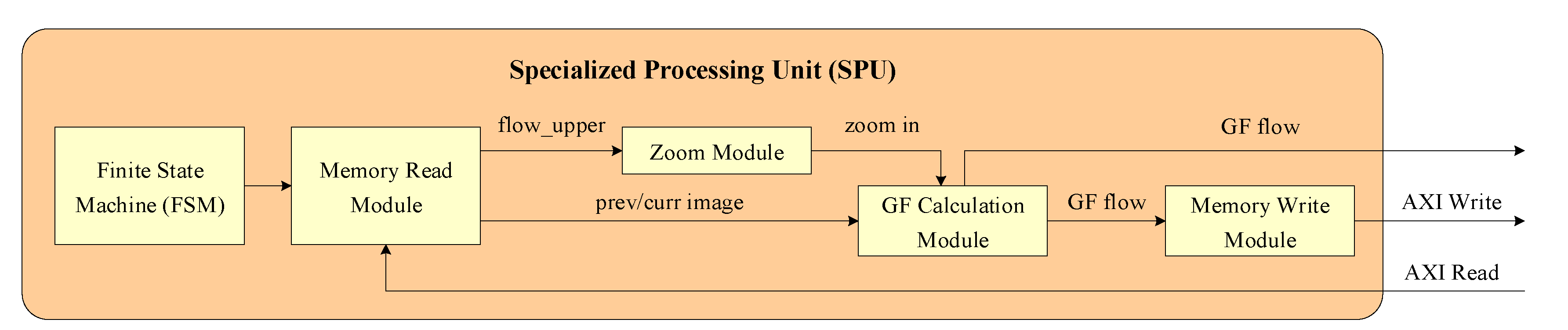
Figure 7.
Architecture of the feature extraction and tracking module
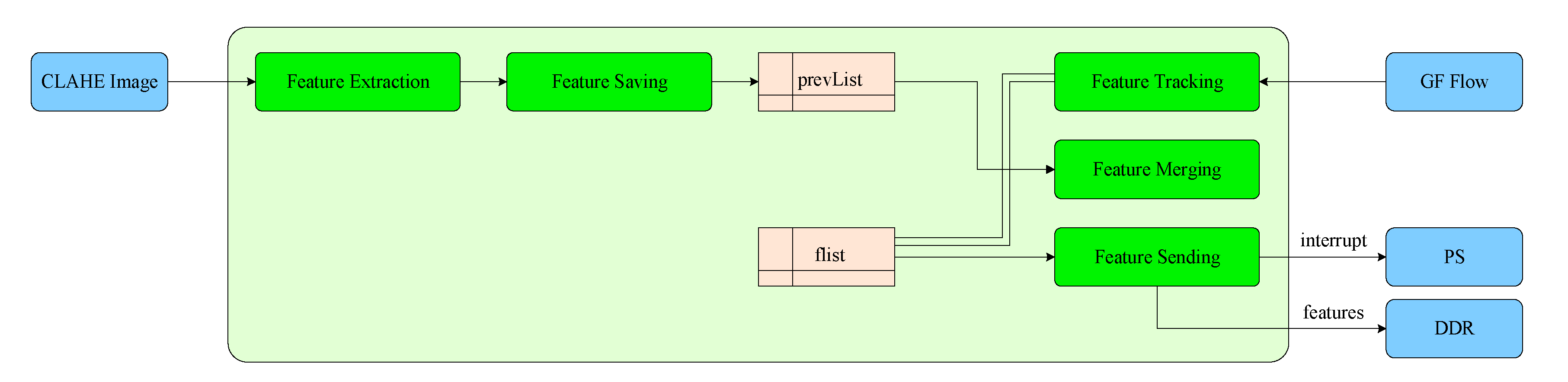
Figure 8.
Coordinate storage of features

Figure 9.
Optical flow tracking and coordinate updating of features
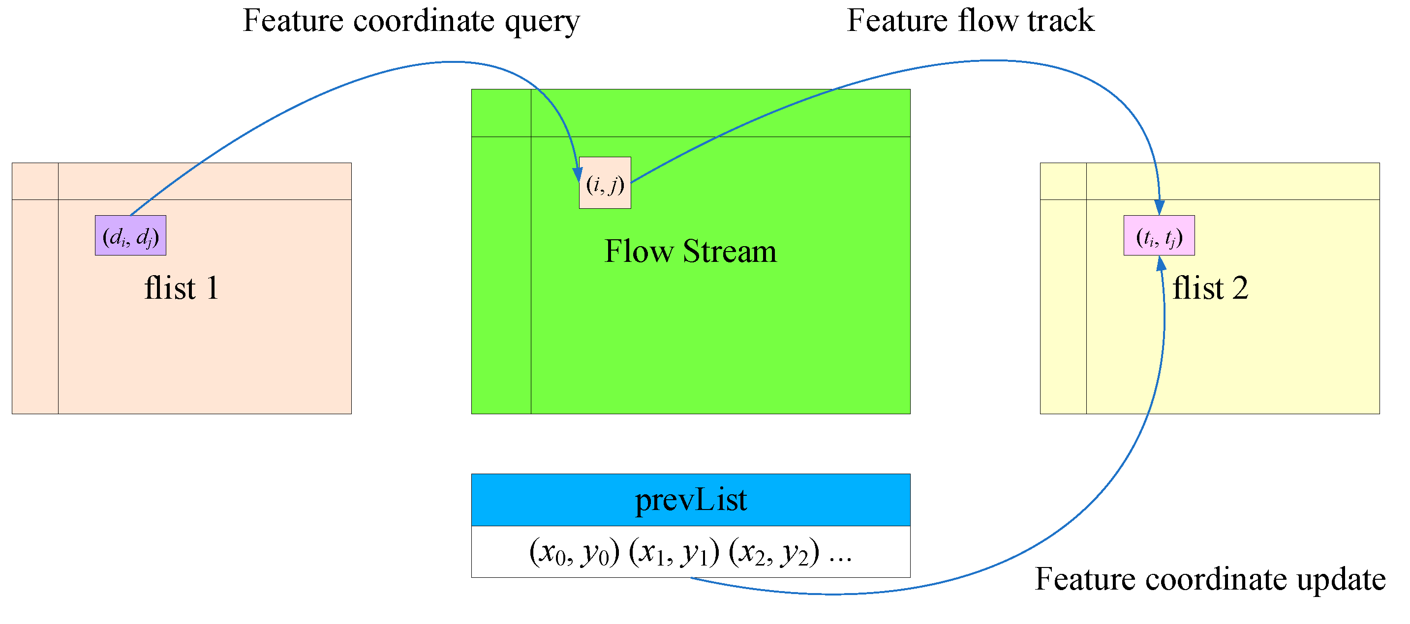
Figure 10.
Workflow of the test benchmark system.
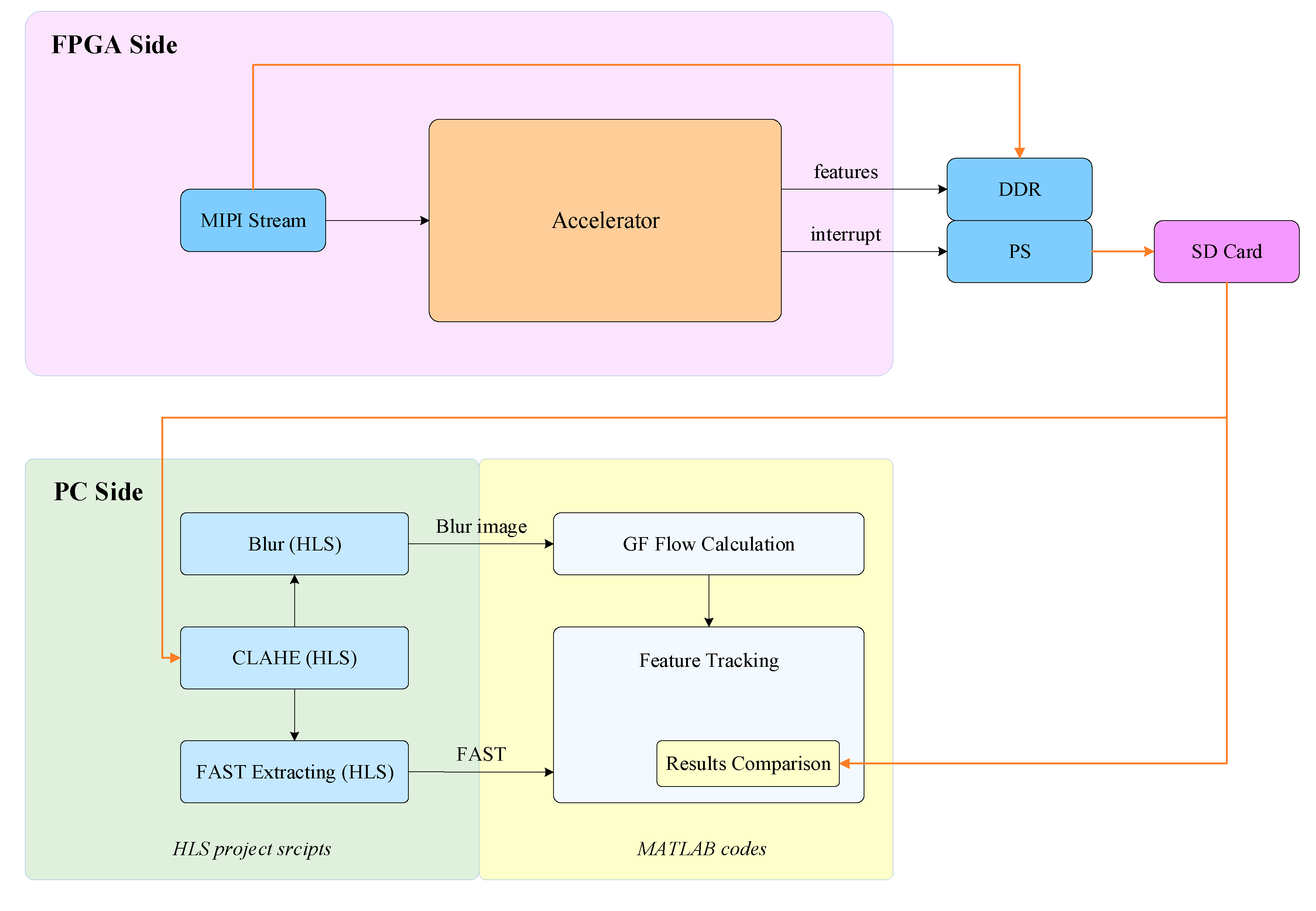
Figure 11.
FAST feature tracking results based on dense optical flow. The processing results of the FPGA accelerator and the MATLAB benchmark completely coincide.
Figure 11.
FAST feature tracking results based on dense optical flow. The processing results of the FPGA accelerator and the MATLAB benchmark completely coincide.
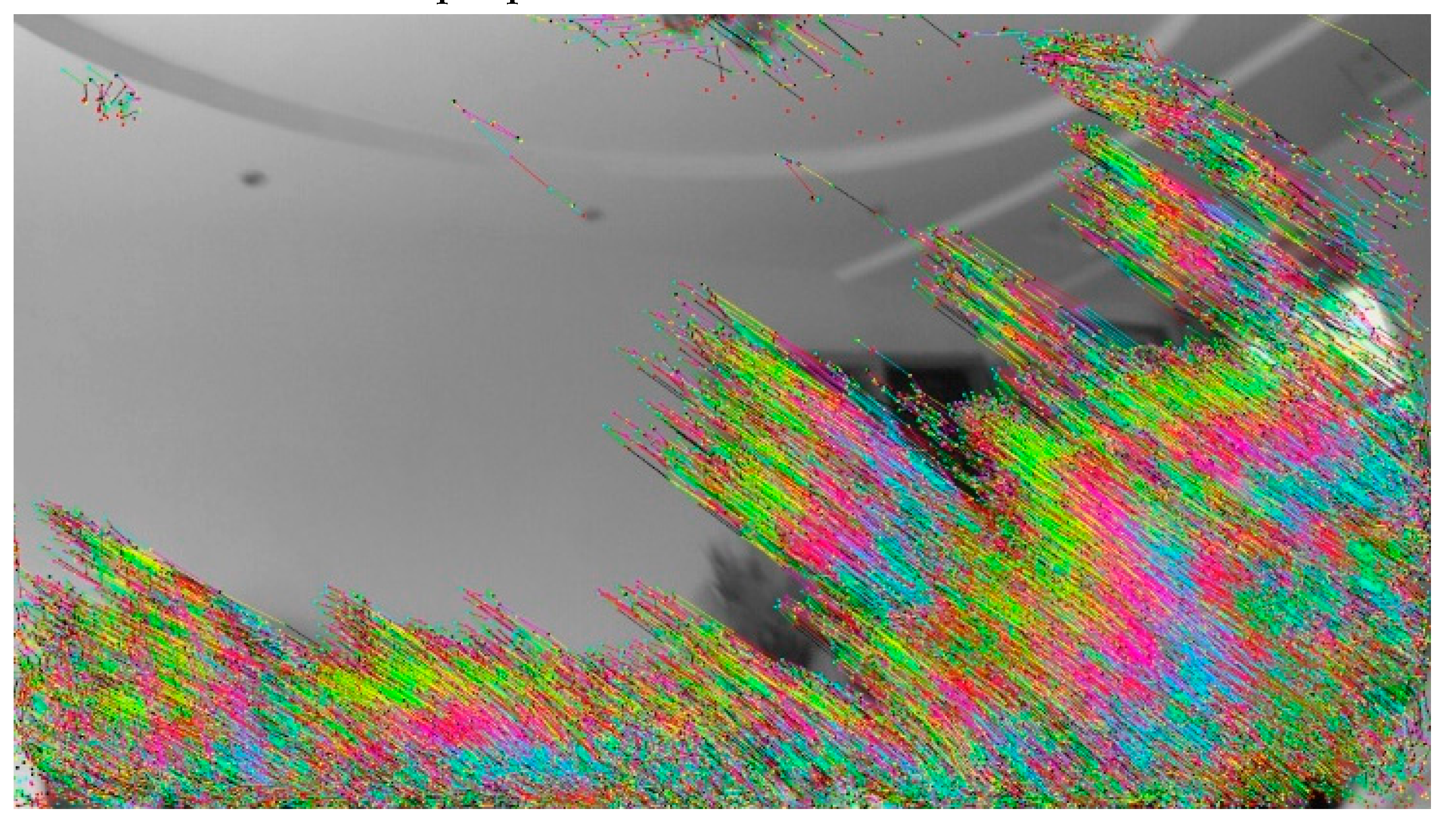

Table 1.
Memory and time usage of the pyramid processing module
| Sequences | |||||
|---|---|---|---|---|---|
| i-1 | i | i+1 | i+2 | i+3 | |
| Memory content | The k-1 st image and its pyramid thumbnails | The k-1 st image and its pyramid thumbnails | The k-1 st image and its pyramid thumbnails | The optical flow between the k-2 st and k-1 st images | |
| The k st image and its pyramid thumbnails | The k st image and its pyramid thumbnails | The k st image and its pyramid thumbnails | The optical flow between the k-1 st and k st images | ||
| The k+1 st image and its pyramid thumbnails | The k+1 st image and its pyramid thumbnails | The k+1 st image and its pyramid thumbnails | |||
| The k+2 st image and its pyramid thumbnails | The k+2 st image and its pyramid thumbnails | ||||
| The k+3 st image and its pyramid thumbnails | |||||
| Processing tasks | Receive the k-1 st image and perform pyramid down; | Calculate the pyramid optical flow of the k-1 st image; Receive the k st image and perform pyramid down; |
Obtain the pyramid optical flow of the k-1 st image; Calculate the pyramid optical flow of the k st image; Receive the k+1 st image and perform pyramid down; |
Obtain the pyramid optical flow of the k st image; Calculate the pyramid optical flow of the k+1 st image; Receive the k+2 st image and perform pyramid down; Calculate the optical flow between the k-1 st and k st images; |
Obtain the pyramid optical flow of the k+1 st image; Calculate the pyramid optical flow of the k+2 st image; Receive the k+3 st image and perform pyramid down Calculate the; optical flow between the k st and k+1 st images. |
Table 2.
Hardware consumption of the proposed FPGA accelerator
| Resource | Available | Utilization | Utilization % |
|---|---|---|---|
| LUT (look up table) | 341280 | 123300 | 36% |
| FF (flip flop) | 682560 | 147172 | 22% |
| BRAM | 744 | 386.5 | 52% |
| URAM | 112 | 68 | 61% |
| DSP | 3528 | 686 | 19% |
| IO | 328 | 82 | 25% |
| BUFG | 404 | 15 | 4% |
| MMCM | 4 | 1 | 25% |
| PLL | 8 | 3 | 38% |
Disclaimer/Publisher’s Note: The statements, opinions and data contained in all publications are solely those of the individual author(s) and contributor(s) and not of MDPI and/or the editor(s). MDPI and/or the editor(s) disclaim responsibility for any injury to people or property resulting from any ideas, methods, instructions or products referred to in the content. |
© 2023 by the authors. Licensee MDPI, Basel, Switzerland. This article is an open access article distributed under the terms and conditions of the Creative Commons Attribution (CC BY) license (http://creativecommons.org/licenses/by/4.0/).
Copyright: This open access article is published under a Creative Commons CC BY 4.0 license, which permit the free download, distribution, and reuse, provided that the author and preprint are cited in any reuse.


