

Submitted:
06 August 2023
Posted:
08 August 2023
Read the latest preprint version here
Abstract
This article studies electrostatic fields and potentials in the presence of conductors and point charges under the framework of solving Laplace’s equation with specifi ed boundary conditions. The results demonstrate that many problems posed and solved in elementary electrostatics through various heuristics such as the method of images, can be more rigorously treated under the solution framework of Laplace’s equation.
Keywords:
potential
; field
; uniqueness
; Legendre polynomial
1. Introduction
Since the times when electricity was studied by rubbing objects like amber and pith [1], empirical formulas have been proposed for the electric force created by a charge at a given distance. By the 18th century, several prominent mathematicians and natural scientists were already aware of the inverse square dependence of the force, and in 1785, French physicist Charles–Augustin de Coulomb published his famous papers [2,4] stating the law now commonly referred to as Coulomb’s law. In modern terminology and notation, the law states that the electric field produced at a point due to a stationary charge q placed at the origin, is given by
or due to a volume charge density distributed over a set by
This formulation provided considerable mathematical advances in electrostatics, and mathematician Carl Friedrich Gauss used Coulomb’s law to formulate the so-called Gauss’s law or Gauss’s flux theorem [5,6], which states that the electric flux through a closed surface is proportional to the total charge enclosed by the surface, or, equivalently in differential form, where is the electrostatic charge density and for a vector field is defined as
With Maxwell’s unification of electromagnetism [8], it was proved that Gauss’s law is more general than Coulomb’s law, and continues to hold beyond electrostatics, even for time-varying fields and charge distributions, and ultimately, from the point of view of modern quantum electrodynamics [10], is a limitation on the degrees of freedom of the photon, the fundamental particle carrying the electromagnetic field.
An electrostatic field satisfying Coulomb’s law (1) is known to be conservative, i.e., the line integral of from a point A to a point B depends only on the vector from A to Potential theory then tells us [12] that any such electrostatic field can be expressed as for some differentiable scalar field Combining this with Gauss’s law yields the Poisson equation [14]
If a region of space has no net charge density, Poisson’s equation reduces to which is the so-called Laplace’s equation [16] arising in diverse application areas such as fluid flow [18], gravitation, electrodynamics [19], and general relativity and cosmology [20]. Due to the broad application and richness of Laplace’s equation, it has spawned a new mathematical field of harmonic functions [21]. In this work, we examine some solutions of Laplace’s equation with various boundary conditions in the context of calculating electric fields and potentials produced by static charge distributions.
2. Laplace’s Equation and Electric Fields
We will solve Laplace’s equation with various boundary conditions to determine the electric potentials (and thereby, the electric fields) produced by various charge distributions and conductors and dielectrics. Since the boundary conditions and charge distributions we will consider will typically have some sort of spherical symmetry, it will be easier to solve Laplace’s equation in the spherical polar coordinates rather than Cartesian coordinates. To facilitate the solution, we first state the following lemma on the form of the Laplace operator in spherical polar coordinates.
Lemma 1.
The Laplacian operator can be represented in spherical polar coordinates as
For completeness, we provide the proof of Lemma 1 in the Appendix.
Remark 1.
Similar to Lemma 1, one can readily establish that the Laplacian operator can be written in the cylindrical coordinates as
We now establish the solution of Laplace’s equation in spherical coordinates with spherical boundary conditions.
Proposition 1.
Consider Laplace’s equation with one or more boundary conditions of the form
for piecewise continuous functions and Then, the solution, if it exists, is of the form
where the constants and are determined by the functions and and the function is the order Legendre polynomial given as [26]
In order to prove Proposition 1, we need 2 additional lemmas, whose proofs are omitted.
Lemma 2
([22]). The solution to the Laplace equation with boundary conditions is uniquely determined by the function f and the radius (). The solution to the Laplace equation with boundary conditions is uniquely determined by the function g and the radius (), up to an additive constant.
Lemma 3
([23]). Given any piecewise continuous function with finitely many discontinuities in the interval consider the sequence of sums
where is theLegendre polynomialdefined as
Then, we have
provided we take
Proof of Proposition 1.
To solve Laplace’s equation with the stated boundary conditions, we will use the so-called separation of variables method [25]. We note that the setting of Proposition 1 is similar to that of Lemma 2, except that the functions and are now functions of only; therefore, by Lemma 2, if we can find a solution matching the boundary conditions, then that would be the unique solution, at most up to an additive constant. To this end, let us define a trial solution of Laplace’s equation of the form where and are twice differentiable functions. Using (2), the Laplace equation then reduces to
or
Now, Equation (6) has to hold for every in the domain, therefore, we must have
where K is a constant independent of the coordinates Examining the equation first, we obtain, through a slight rearrangement,
Writing enables us to write and the equation therefore reduces to
Now, dividing throughout by writing and noting that
the equation becomes, in terms of as the independent variable,
Equation (7) is the Legendre equation [26] with For non-integer the solutions to Legendre’s equation are power series with radius of convergenece smaller than For the current problem, however, the domain is Therefore, the only possible solutions to (7) that would make the trial solution valid, should be polynomials. Through the application of Sturm–Liouville theory (see, for example, [23]), we can conclude that the solutions are indeed polynomials when l is a non-negative integer. Therefore, for the trial solution to be valid, we must have for a non-negative integer and the corresponding solution of the equation becomes
up to a multiplicative constant. To tackle the r equation, writing enables us to write and a change of independent variable to enables us to write the v equation as
and replacing r with leads to
which simplifies to
From elementary calculus, Equation (9) has the general solution of the form
where and are solutions of the quadratic equation We immediately obtain and which yields the solution
and the solution to the r equation then becomes
Finally, noting that since the Laplace equation is linear, any linear combination of a set of valid solutions will also be a solution, we come up with the largest set of soltuions that the trial solution enables us to get, by combining (10) and (8):
Now, by uniqueness (Lemma 2), if we can find constants matching the boundary conditions (4) and/or (5), then (11) with the determined constants will be the unique solution to the problem. Let us now focus on the boundary conditions (4). The result will similarly follow for the boundary conditions (5). Since is a piecewise continuous function, by the completeness of Legendre polynomials (Lemma 3), there exist constants for which
More specifically, we have, in this case,
Note that at least 2 such boundary conditions are needed to uniquely determine the constants and For such consistent boundary conditions, (11) with the constants and determined by the boundary conditions (12) is the unique solution to the Laplace equation. □
We will now directly use Proposition 1 to calculate electric potentials (and, thereby, electric fields) rigorously for various electrostatics problems commonly posed in many textbooks (see, for example, [19]).
2.1. Conducting Sphere in Uniform Electric Field
Consider a conducting sphere of radius (with center at the origin) placed in a uniform electric field Without loss of generality, let If a unique solution exists in the region it must only be determined by the vector and therefore, must be independent of (This property is referred to as azimuthal symmetry.) We can then write a trial solution as
which yields
Since the conductor is finite, the distortion caused by it to the electric field is local and therefore, as the electric field must approach We thus have which is only possible if for and The solution then becomes
for some constants Now, for a conductor, the electric field at the surface is purely along the normal to the surface, and therefore, we have
which, combining with (13), yields
for This is satisfied if and for and the solution therefore becomes
which yields the electric field
Note that (14) satisfies as required. However, the constant is still undetermined. It is a measure of the state of the conductor, as can be seen from the following. From (14), we have
Since the electric field inside a conductor is zero, we have that the surface charge density induced on the sphere is given by The total charge on the conductor is then given by
which enables us to finally write the electric field in terms of the physical invariants of the system as
This essentially says that the total net charge on the conductor gets distributed in such a way as to produce the same field (outside the conductor) as a point charge placed at the center. In particular, if we place an uncharged conductor inside a uniform electrostatic field then the final electrostatic field will be given by
We finally note that this expression for the electric field is “coordinate free” in the sense that it is only a function of the vector and the radius vector at each point, the latter of which essentially encodes the position of the sphere.
Figure 1 illustrates the electric field lines on a vertical plane (i.e., containing the z axis) obtained from the electric field in (17). As expected, far away from the sphere, the lines are vertical, while close by, they are “distorted” by the presence of the conductor. We also note that the field lines always enter and leave the sphere normally, and field abruptly drops to 0 as soon as we cross the boundary into the conductor. Finally, the field lines are seen to be the densest around the poles of the conductor (), which can also be verified analytically from Equation (17). An analytical derivation yields a maximum field strength of
2.2. Conducting Sphere Near a Point Charge
Consider a conducting sphere of radius (with center at the origin) placed near a point charge q located at with (see Figure 2). Since the conducting sphere is an equipotential, let it be at potential The overall potential for can be written as where is the potential due to the charge q and satisfies Laplace equation with appropriate boundary conditions.
To determine these boundary conditions, we note that the potential due to the charge q at a point on the sphere (assuming the boundary conditions ) is given by Coulomb’s law as
Therefore, satisfies the boundary condition
Writing a trial solution as
we observe that since we have the boundary conditions we must have for all To obtain the coefficients using (18), we need the following lemma.
Lemma 4
Remark 2.
Since we have and we can use Lemma 4 to rewrite (18) as
Therefore, by the uniqueness theorem (Lemma 2), the coefficients are given by
The general solution is thus given by
for Equation (23) can be written in a more illuminating form as
The overall potential is then given by
The potential (25) is the same as that produced by the charge q at together with “virtual” charges at and at the center of the conducting sphere. This can also be obtained through the so-called method of images as used in many treatments of this topic [19]. Equation (25) also enables us to write the surface charge density on the sphere as
The charge density (26) can be integrated to obtain the total charge on the sphere as
Writing we have
We can then continue (27) as
Equation (29) is often interpreted (see, for example, [19,29]) as the sum of the image charges and
2.3. Uniform Dielectric Sphere in Uniform Electric Field
Consider a sphere of radius made of a linear deielectric material of electric susceptibility (with center at the origin) placed in a uniform electric field Without loss of generality, let We now wish to find the field both inside and outside the sphere. As we shall see later (cf. Remark 4), this situation can be thought of as a generalization to the problem studied in Section 2.1. As argued in Section 2.1, this problem exhibits azimuthal symmetry since the boundary conditions are independent of We can then write trial solutions for the potentials inside and outside the sphere as
We will now discuss the boundary conditions to this problems, which are what will turn out to cause the crucial differences in the solutions for this case. First, as argued in Section 2.1, the electric field must approach as and we therefore conclude that for and Further, since the field inside the sphere is finite, must have finite derivatives as and (30) then leads us to conclude that for all Equation (30) and (31) then enable us to write down a global trial solution as
By the continuity of V at the surface of the dielectric, the two expressions in (32) must match at Rearrangement leads to
Using the completeness of Legendre polynomials (Lemma 3) and noting that Equation (33) enables us to write
Finally, we come to the behavior of the electric field at the surface of the dielectric, which will yield additional boundary conditions and will be determined by the properties of the dielectric. The surface density of bound charges on the dielectric can be written as
This bound charge density, however, is also given by the radial component of the polarization vector i.e., Finally, since the material is a linear dielectric, we have for We therefore have
Equations (37) and (38) enable us to write
Using Lemma 3 again, the boundary condition (39) enables us to write
For (36) and (42) can simultaneously hold only if Moreover, (35) and (41) enable us to solve for as
i.e.,
This immediately yields
and we can finally write down the full solution (32) as
The potential (43) yields the electric field
The electric field inside can then be written as
which turns out to be uniform. The field outside can be written as
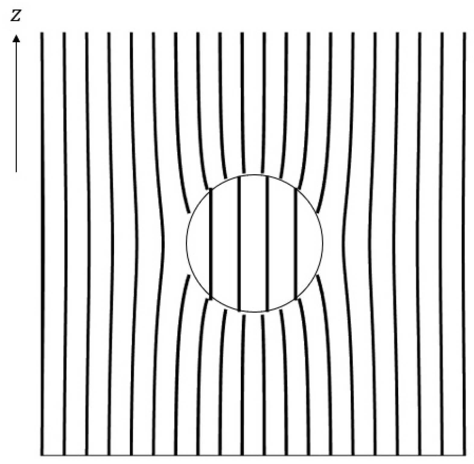
Figure 3 illustrates the electric field lines on a vertical plane (i.e., containing the z axis) obtained from the electric field in (46) and (44). As expected, far away from the sphere, the lines are vertical, while close by, they are “distorted” by the presence of the dielectric. We also note that there is a discontinuity of the field at the boundary of the dielectric, but unlike Figure 1 in Section 2.1, the field inside the dielectric is nonzero. Finally, the field lines are no longer orthogonal to the surface of the dielectric; the field can have a tangential component and electrostatic conditions can still be maintained.
Remark 3.
We note that the field when an uncharged conductor is placed in a uniform electric field (cf. (17) in Section 2.1) can also be written as
Both (47) and (45) can be compared to the field of a dipole placed at the origin (see, for example, [19]):
This suggests that a sphere made of a conductor or a linear dielectric material placed in an uniform electrostatic field acquires a dipole moment equal to
The polarization is defined as dipole moment per unit volume, therefore this suggests that the spheres acquire polarizations and The electric susceptibility therefore, can be interpreted as a parameter quantifying the amount of “freedom of movement” of charges inside a metrial – in a conductor they have perfect freedom of movement (i.e., ability to polarize), enabling complete cancellation of the electric field, but in a dielectric sphere, the polarization is times relative to a conductor.
Remark 4.
We note that all results in Section 2.1 follow from those in this section by taking This shows that in electrostatics, in many situations a conductor can be thought of as a dielectric within infinite susceptibility. Taking this limit for (44) for the field inside the dielectric immediately recovers the result that the field is zero inside the conductor.
Remark 5.
Note that in this section, we tacitly assumed that the dielectric is uncharged when we equated (37) and (38). The dielectric, in fact, could have a “free” surface charge density which would then have to be taken into account at that step. However, because charges cannot move about freely in a dielectric, unlike in a conductor, the complete charge density would have to be specified for this problem to have a unique solution.
3. Discussion
The general setup described in this work can be used to find potentials and fields for a wide range of charge distributions commonly used to demonstrate the “method of images” in electrostatics texts. A popular and elementary problem setup not explored in this work is the infinite conducting plane near a point charge which can be similarly solved, but in the cylindrical coordinates using (3). For a detailed account of the history and development of Laplace’s equation and solution techniques in the context of electrostatics, we refer the reader to [1].
Appendix A. Proofs
Proof of Lemma 1.
We first establish some preliminary results that will make the proof considerably easier. The relations between Cartesian and spherical polar coordinates can be written [31] as
and
where is the four-quadrant inverse tangent defined as the real number satisfying and Treating the spherical unit vectors and as functions of we can then write
and
Equations (A3)–(A5) can be easily inverted to yield
or, more compactly,
One can verify that the matrix M is orthogonal, i.e., Finally, the infinitesimal line element can be written in spherical spherical polar coordinates as
where follows from Equations (A3)–(A5). This also leads us to conclude immediately, that the infinitesimal volume element (since and are orthonormal) is given by
Now, with these preliminaries established, let f be a differentiable scalar field. We have
Now, writing and using the gradient theorem [12] (A7) and (A8), we have
This implies that
Equation (A9) also implies that
or in other words,
We can write (A10) as the three scalar equations
Now, let be a differentiable vector field. We have
which leads to
or, since M is orthogonal,
We can write (A14) as the three scalar equations
Using eqns (A11)–(A13) and (A15)–(A17), collecting terms, and simplifying, we obtain
Combining (A9) and (A18), we can then write, for a twice differentiable scalar field
where follows from (A18), by using Equation (A19) establishes the result. □
References
- Brian Baigrie, Electricity and Magnetism: A Historical Perspective (Greenwood Press, 2007), pp. 7–8.
- Charles–Augustin de Coulomb, “Premier mémoire sur l’électricité et le magnétisme”, Histoire de l’Académie Royale des Sciences, 1785.
- Nadim Ghaddar, Shouvik Ganguly, Lele Wang, and Young-Han Kim, “A Lego-Brick Approach to Coding for Asymmetric Channels and Channels with State”, Proceedings of the International Symposium on Information Theory (ISIT), pp. 1367–1372, 2021.
- Charles–Augustin de Coulomb, “Second mémoire sur l’électricité et le magnétisme”, Histoire de l’Académie Royale des Sciences, pp. 578–611, 1785.
- Shouvik Ganguly and Young-Han Kim, “Capacity Scaling for Cloud Radio Access Networks with Limited Orthogonal Fronthaul”, Proceedings of the International Symposium on Information Theory (ISIT), pp. 1472–1476, 2019.
- Carl, F. Gauss, “Theoria attractionis corporum sphaeroidicorum ellipticorum homogeneorum methodo nova tractata”, Gauss, Werke V, p. 1.
- Nadim Ghaddar, Shouvik Ganguly, Lele Wang, and Young-Han Kim, “A Lego-Brick Approach to Coding for Network Communication”, arXiv:2211.07208v3 [cs.IT], 2022.
- James Clerk Maxwell(1865), “A dynamical theory of the electromagnetic field”, Philosophical Transactions of the Royal Society of London, 155, pp. 459–512.
- Shouvik Ganguly and Sridip Pal, “Bounds on the Density of States and the Spectral Gap in CFT–2”, Phys. Rev. D 101(14):106022, pp. 1–4, May 2020.
- Richard, P. Feynman, “Space–Time Approach to Quantum Electrodynamics”, Phys. Rev. 76(6), pp. 769–789, 1949.
- Shouvik Ganguly, Lele Wang, and Young-Han Kim, “A Functional Construction of Codes for Multiple Access and Broadcast Channels”, Proceedings of the International Symposium on Information Theory (ISIT), pp. 1581–1586, 2020.
- P. R. Garabedian and M. Schiffer, “On existence theorems of potential theory and conformal mapping”, Annals of Mathematics 52(1), pp. 164–187, 1950.
- Shouvik Ganguly and Lele Wang, “Sliding-Window Gelfand–Pinsker Coding: General K-User Broadcast Channels”, Proceedings of the IEEE Information Theory Workshop (ITW), pp. 1–5, 2020.
- Siméon Denis Poisson, “Mémoire sur la théorie du magnétisme en mouvement”, Mémoires de l’Académie Royale des Sciences de l’Institut de France 6, pp. 441–570, 1823.
- Shouvik Ganguly and Young-Han Kim, “On the Capacity of Cloud Radio Access Networks”, Proceedings of the International Symposium on Information Theory (ISIT), pp. 2063–2067, 2017.
- R. Courant and D. Hilbert, “Methods of Mathematical Physics”, Interscience, New York, 1966.
- Shouvik Ganguly, Seung-Eun Hong, and Young-Han Kim, “On the Capacity Regions of Cloud Radio Access Networks with Limited Orthogonal Fronthaul”, IEEE Trans. Inf. Theory 67(5), pp. 2958–2988, May 2021.
- Richard, P. Feynman, Robert B. Leighton, and Matthew Sands, The Feynman Lectures on Physics, Vol. 2, Chap. 12 (Addison-Wesley, 1964).
- David, J. Griffiths, Introduction to Electrodynamics (Boston:Pearson, 2013).
- S. Persides, “The Laplace and Poisson equations in Schwarzschild’s space–time”, Journal of Mathematical Analysis and Applications 43(3), pp. 571–578, 1973.
- David Gilbarg and Neil, S. Trudinger, Elliptic Partial Differential Equations of Second Order (Berlin: Springer, 2015).
- G. Barton, Elements of Green’s Functions and Propagation: Potentials, Diffusion and Waves (Oxford: Oxford Science Publications, 1989).
- Augusto, B. d’Oliveira, Ed Gerck, and Jason A. C. Gallas, “Solution of the Schrödinger equation for bound states in closed form”, Phys. Rev. A 26:1(1), June 1982.
- S. Ganguly, K. Sahasranand, and V. Sharma, “A New Algorithm for Distributed Nonparametric Sequential Detection”, Proceedings of the IEEE International Conference on Communications (ICC), pp. 1409–1415, 2014.
- Erwin Kreyszig, Advanced Engineering Mathematics (3rd ed). New York: Wiley, 1972.
- George, B. Arfken and Hans J. Weber, Mathematical Methods for Physicists (Elsevier Academic Press, 2005).
- Richard Courant, Differential and Integral Calculus, Vol. 1 London: Blacktie & Son Limited, 1961.
- Jongha Jon Ryu, Shouvik Ganguly, Young-Han Kim, Yung-Kyun Noh, and Daniel D. Lee, “Nearest Neighbor Density Functional Estimation based on Inverse Laplace Transform”, IEEE Trans. Inf. Theory 68(6), pp. 3511–3551, June 2022.
- J. D. Jackson, Classical Electrodynamics (3rd ed.) (New York:Wiley, 1999).
- S. Ganguly, K. Sahasranand, and V. Sharma, “A New Algorithm for Nonparametric Sequential Detection”, Proceedings of the National Conference on Communications (NCC), India, pp. 1–6, 2014.
- P. M. Morse and H. Feshbach, Methods of Theoretical Physics, Part I (New York: McGraw–Hill, 1953), p. 658.
- Nadim Ghaddar, Shouvik Ganguly, Lele Wang, and Young-Han Kim, “A Lego-Brick Approach to Lossy Source Coding”, Proceedings of the 17th Canadian Workshop on Information Theory (CWIT), pp. 45–50, 2022.
Figure 1.
Electric field lines.
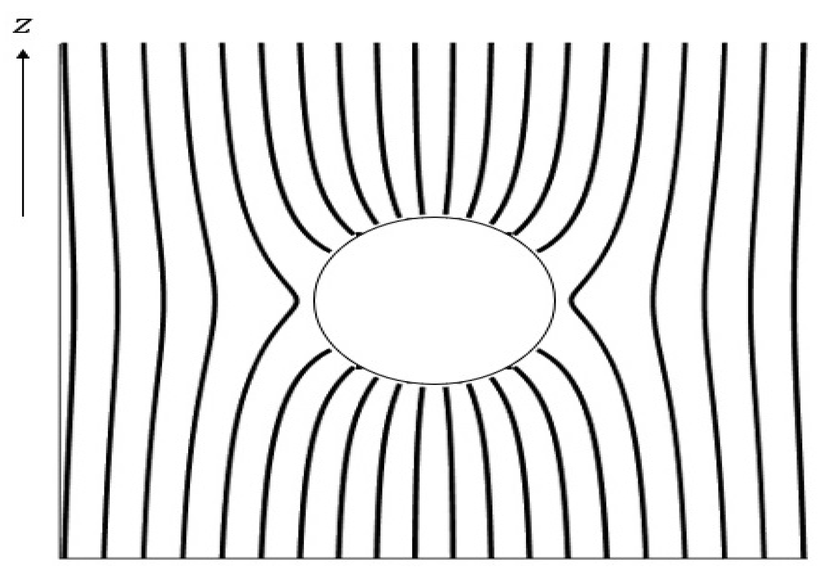
Figure 2.
Conducting sphere near a point charge.
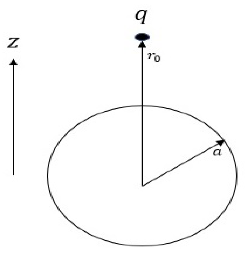
Figure 3.
Electric field lines.
Disclaimer/Publisher’s Note: The statements, opinions and data contained in all publications are solely those of the individual author(s) and contributor(s) and not of MDPI and/or the editor(s). MDPI and/or the editor(s) disclaim responsibility for any injury to people or property resulting from any ideas, methods, instructions or products referred to in the content. |
© 2020 by the author. Licensee MDPI, Basel, Switzerland. This article is an open access article distributed under the terms and conditions of the Creative Commons Attribution (CC BY) license (https://creativecommons.org/licenses/by/4.0/).
Copyright: This open access article is published under a Creative Commons CC BY 4.0 license, which permit the free download, distribution, and reuse, provided that the author and preprint are cited in any reuse.


