
Submitted:
28 July 2023
Posted:
31 July 2023
You are already at the latest version
Abstract
A major driver of declining biodiversity is landcover change leading to loss of habitat. Many studies have estimated large-scale declines in biodiversity, but loss of biodiversity at a local scale due to the immediate effects of development have been poorly studied. California, in particular, is a biodiversity hotspot and has rapidly developed; thus, it is important to understand the effects of development on wildlife. Here, we conducted reconnaissance surveys -- a type of survey often used by consulting biologists in support of environmental review of proposed projects -- to measure changes in relative abundance and richness of vertebrate species in response to urban development. We completed 2 reconnaissance surveys at each of 52 control sites that remained undeveloped at the times of both surveys, and at each of 26 impact sites that had been developed by the time of the second survey. We completed the surveys as part of a before-after, control-impact (BACI) experimental design. Our main interest was on the interaction effect between the before-after phases and control-impact treatment levels, or on the impact of development. We also tested for effects of survey duration, years intervening the surveys in the before and after phases, project area size, latitude, degree of connectedness to adjacent open space, and whether the site was a redevelopment site, infill or not infill. After development, the average number of vertebrate wildlife species we detected declined 48% within the project area, and 66% within the bounds of the project sites. Further, the average number of vertebrate animals we counted declined 90% within the project area, and 89% within the bounds of the project sites. Development impacts measured by the mean number of species detected per survey were greatest for amphibians (-100%), followed by mammals (-86%), grassland birds (-75%), raptors (-53%), special-status species (-49%), all birds as a group (-48%), non-native birds (-44%), and synanthropic birds (-28%). Our results indicated that urban development substantially reduced vertebrate species richness and numerical abundance, even after richness and abundance had likely already been depleted by the cumulative effects of loss, fragmentation, and degradation of habitat in the urbanizing environment. Cumulative effects monitoring is needed, and so are conservation measures to mitigate the effects of urbanization.
Keywords:
BACI experiment
; birds
; California
; development
; reconnaissance survey
; species richness
; urbanization
; vertebrate wildlife
1. Introduction
Urbanization has been defined as “the process of human settlement that gradually transforms uninhabited wildlands into lands including some degree of relatively permanent human presence” [1]. Urban growth profoundly affects the availability and condition of natural resources, and within its immediate area it often fragments and degrades habitat and simplifies biological species composition [2], as well as homogenizes species composition of plants [3] and wildlife [4,5,6,7,8] and land-cover composition, landscape structure, and ecosystem functions [9]. Urban areas also reduce avian taxonomic diversity [10,11]. In short, urbanization diminishes biodiversity, which is intrinsically valuable but also essential to human quality of life [11,12]. “Biodiversity is the variety of life” [11], ranging from the microbial to biome, from genetics to phenotypes, and including ecological processes of storages, flows and interactions. It is too complex to measure on the whole, so ecologists simplify measures of biodiversity with indicators such as populations, species and habitats, which are also better documented and understand than most other potential measures of biodiversity [12]. Biodiversity is on the decline [12]. A major driver of declining trends in biodiversity within metropolitan areas is the extent of landcover that serves as habitat [8].
Habitat is that part of the environment that is used by members of a species [13,14]. But when that part of the environment is converted to one or more buildings, associated impervious surfaces (parking lots), and lawn or ornamental vegetation as cover on the residual ground surface, along with all of the noise, light and air pollution and sources of mortality that accompany urban development, habitats of many species are lost [15]. In the context of a city or metropolitan area, habitat loss likely also includes habitat fragmentation which results in a net loss of productive capacity of a species that exceeds that of habitat loss alone [16]. Because habitat loss and habitat fragmentation have progressed rapidly around the world, the effects of these processes on wildlife are also advancing rapidly [17]. Already, there have been documented genetic effects [18], and shifts in community composition and in physical and behavioral morphologies of species remaining within the areas of urbanization [15,19].
Many species of vertebrate wildlife have been in numerical decline across North America [20]. These declines have been attributed to multiple causal factors, but habitat loss and habitat fragmentation have usually been hypothesized as the leading causes of declines. Habitat loss is readily believable because we can see and measure the extent to which we have been clearing natural vegetation to make way for agricultural, industrial, commercial and residential uses and all of their connecting roads and highways, pipelines and electrical transmission lines. Less measured, however, has been the actual changes in wildlife species composition and numerical abundance on sites where natural or managed vegetation has been removed to accommodate anthropogenic structures.
To indicate the effects of habitat loss due to urbanization, correlational analysis has been performed on bird species richness with variables intended to measure urbanization and degrees of departure from natural conditions [21,22,23,24]. In one study, birds were sampled in forest patches within an urban environment to test for correlations with patch size and degrees of disturbance [25]. Similarly, Crooks et al. [5] assessed the effects of urbanization by comparing bird species richness and abundance sampled in urban areas to samples taken from small and large habitat fragments and larger core areas of habitat. In another study, bird species richness was sampled along a gradient of urbanization, and it was assumed that the bird community sampled in the least urbanized end of the gradient best represented the pre-development bird community [26]. Investigators in another study estimated relative species richness of birds as an indicator of the effects of urbanization by comparing sampled species richness to a specified reference community or to the regional pool of species that should have existed prior to development [27]. The reference community would indicate a baseline ecological integrity, or the biological species assemblage during pristine conditions, sensu [28]. This approach, however, did not directly measure the effects of urbanization because it assumed the pristine reference community was accurately specified. The effects of habitat loss due to development have more often been assumed or inferred from gradient experiments, but perhaps directly measured only rarely [29,30].
One study that directly measured how construction of buildings affected bird species richness and abundance found no effect [30]. However, the study’s surveys were brief (10 min) and extended only to 30.5 m on a single study site. The study lacked the experimental design elements of replication, control, and sufficient scale needed to achieve the study’s objective. Another study that measured the effects of construction grading on the local woodland bird community initially documented equivocal impacts [29]. This study, however, provided greater insight into impacts because it’s sampling covered a larger area and twice the time as the other study. Grading displaced birds to adjacent habitat, where temporary crowding inflated the investigator’s bird counts. After another year, the effect of crowding was lost and a net loss of birds was realized [29]. Rare are long-term studies or experimental studies including controls to more directly test for the effects of urbanization [1].
Marzluff et al. [1] recommended that research to test for the effects of urbanization on wildlife should take advantage of the opportunities for experiments that urban development brings. Advanced knowledge of where and when the next projects are to be developed should give biologists opportunities to design experiments, which is just what Scott [29] did. We saw such an opportunity, discussed below, but we note that sites proposed for development are typically already far removed from the ecological integrity of pristine environmental conditions that preceded urbanization in the area. Realistically, the opportunities for experiment based on advanced knowledge of where development will extend must begin with baseline environmental settings that are highly disturbed or consist of habitat fragments in an urbanizing landscape [29]. What can be measured in such experiments are only partial, final-stage effects of urbanization on plants and wildlife.
We often survey for wildlife at sites that are proposed for development of anthropogenic structures in California. The California Environmental Quality Act (CEQA) requires the characterization of the existing environmental setting. This characterization informs the public and decision-makers of what is at stake in the face of the proposed project, and it serves as the baseline from which to opine on or predict project-caused impacts and to formulate appropriate mitigation measures to avoid, minimize, reduce, rectify or offset the impacts. To characterize the wildlife community as part of the existing environmental setting, consulting biologists usually perform what are referred to as reconnaissance surveys, otherwise known as general biological surveys. These surveys typically include one or more biologists walking over the project site or scanning the site from vantage points. The surveys vary in duration, typically lasting 1 to several hours. These surveys have not relied on fixed time-spans, and have lacked any clear stopping rules other than the biologists finished walking the pedestrian transects across the project area, whether those transects were evenly spaced or meandering. Having worked for environmental consulting firms in the past, in our experience the primary stopping rule is budget, although it was not always clear why a survey would come to an end at a particular site. We have seen no evidence that the stopping rules for reconnaissance surveys are results-based, as advocated by [31].
To check on the veracity of the results and interpretation of reconnaissance surveys completed by consulting biologists, we were often hired by parties other than the project applicants or the permitting agencies to also survey the project sites. One difference between the consultants’ surveys and ours is that the consultants surveyed directly on the project sites whereas we nearly always were constrained to survey from the project’s periphery because we were rarely granted access to the site’s interior. But this difference accommodated our post-construction, repeat surveys of sites that had been developed, because these developed sites could only be performed on the project site’s periphery due to the new physical presence of one or more buildings. As for the veracity of the survey findings of consulting biologists, they are of no relevance to the objectives of the study we present here.
We managed our surveys of project sites in the framework of a before-after, control-impact experiment to measure average project impacts to wildlife. Our control sites were those project sites that had not been developed prior to our second survey which represented the after phase of the experiment, and the impact sites were those sites that had been developed by the time of our second survey. Our baseline settings in the before-phase surveys were far from pristine at most project sites, but they nevertheless served as baselines for measuring changes brought by construction of buildings to the number of vertebrate species detected and to our counts of live animals, which we intended to indicate respectively as species richness and relative abundance. We use the term “indicate” here because we recognize that we did not truly measure species richness nor true abundance, as multiple potential biases and error prevented such measurement [32]. On the other hand, our surveys were of sufficient duration to detect most of the diurnal bird species that would have been available to us at each site at the times of our surveys [33]. Our primary objectives were to measure changes in 1) the number of vertebrate species detected, 2) the number of species uniquely detected at a site in one phase relative to the species detected in the other phase, 3) counts of live animals, and 4) percentage of project sites within each BACI treatment group where we detected each species. Our secondary objective was to explore whether other measured variables might explain the residual variation from the Analysis of Variance (ANOVA) model used to test the BACI hypotheses for main and interaction effects. We additionally tested for effects of survey duration, years intervening the surveys in the before and after phases, project area, latitude, degree of connectedness to adjacent open space, and whether the site was a redevelopment site, infill or not infill.
2. Materials and Methods
2.1. Study Area
Our study sites were clustered in the Sacramento and Central Valleys, the San Francisco Bay Area, and the coastal region of southern California (Figure 1). Each of these sites had been selected by our clients for reasons that had nothing to do with our BACI experiment. We later added follow-up surveys where practical and when we could closely match the date and start time of the initial surveys. Twenty-six of the sites had been developed by the time of our follow-up surveys, whereas 52 sites remained undeveloped. Developed sites were those for which the intended structures of the project were completely or nearly completely built, but they did not have to be occupied (some structures remained vacant for extended periods) (Figure 2, Figure 3 and Figure 4). Thirty-five of the sites were within or peripheral to existing urban, commercial or industrial areas, but 30 were located on agricultural or desert landscapes (Appendix A). The condition of most of our study sites was poor to moderate at the times of our initial surveys, as most sites had been disturbed by mechanical clearing of vegetation (Figure 5), use of the sites as construction laydown areas in support of development of adjacent properties, frequent fires, off-road vehicle use, non-native plant species composition (Figure 6), encroachment of non-native vertebrate species from surrounding urbanized areas (Figure 7), and other forms of pollution, e.g., dumping of waste materials and mowing for weed abatement. Only 4 of the sites were surrounded on all sides by open space. Nevertheless, wildlife utilized all of the study sites we surveyed. Study sites ranged from 0.526 ha to 1,549 ha (mean = 91.26 ha, SD = 255.44 ha), with the 2 largest study sites consisting of natural reserves that we used as control sites.
2.2. Reconnaissance Surveys
We performed what are referred to in California as reconnaissance surveys, also known as general biological surveys. We intentionally implemented the same methodology as used by environmental consultants when they perform reconnaissance surveys. In these surveys, all species are recorded if detected by visual or auditory means or by sign such as burrows or tracks or scat. Wildlife recorded included birds, mammals, amphibians and reptiles. We surveyed by walking the perimeter of the site, or by a stationary vantage point, where we scanned for wildlife with the use of binoculars. In most surveys, we recorded the time within the survey when a new species was detected, whether the species was on the project site or in the surrounding area, and the approximate abundance of that species.
Reconnaissance surveys are unbound by time, but typically last between 1 and several hours. Our surveys differed from the surveys of environmental consultants only in three ways: (1) we were usually restricted from accessing the interiors of project sites, (2) we used full-frame cameras fitted with telephoto lenses to help detect and identify wildlife to species, and (3) our stopping rule was results-based, and increasingly so the more surveys we had completed; however, in the cases of our second surveys to represent the after phase of the experiment, our stopping rule was the time it took to record all of the species that had been recorded in each initial survey. Experience with these surveys led us to stop our initial survey at each project site once our species detection rate declined to about one new species per 20 or 30 minutes, similar to the rule advocated by Watson [31]. These lower detection rates typically coincided with increasing heat of the day or oncoming darkness of the evening.
We recorded temperature, wind and sky condition at the start and end of most surveys, and we recorded ground conditions at all sites at the time of each survey. We categorized an urban setting index for each site as 0 = largely non-urbanized, 1 = urban infill, and 2 = redevelopment. We rated connectivity of project site borders to adjacent open space (including agriculture) as 0%, 10%, 25%, 50%, 75%, and 100%. We categorized sites as having undisturbed vegetation; evidence of disturbance over the last 5 years or so; ruderal; mowed; neglected by accumulation of trash, construction debris, waste soil or machine parts; neglected by cessation of irrigation; burned; disked; graded; construction ongoing; or constructed, as well as combinations of the foregoing categories. From these categories, we rated sites for level of disturbance as 1 = natural and biologically intact with no more than small patches of non-native vegetation; 2 = mostly intact with some native and some non-native vegetation, or all native with some past ground disturbance; 3 = modified (disked or highly disturbed) in the past but with substantial extent of vegetation such as patches of shrubs or scattered trees; 4 = landscaped parks or golf courses; 5 = agriculture including orchards and vineyards; 6 = agriculture including row crops; 7 = parking lot with mature shrubs or trees, and where buildings do not cover the entire site; 8 = highly modified with little vegetation remaining; 9 = compacted, pervious ground with no vegetation remaining; 10 = impervious ground with no vegetation remaining; 11 = constructed buildings. We further categorized site conditions to represent the intensity of actions that likely would have suppressed wildlife as 0 = none evident, 1 = low (ruderal, cleared fire break), 2 = routine disturbance, 3 = moderate (mowed, neglected), 4 = earlier intense (near-recent grading, regrowth after disking), 5 = intense (cleared, disked, disked and neglected), and 6 = very intense (converted to crop, graded, constructed).
Beginning in January 2020, we began to resurvey sites of proposed building projects that we had originally surveyed during the same time of year and about the same time of day between 1 and 19 years earlier. In addition to starting the repeat survey as close to the original start time as possible, we surveyed for the same duration and using the same person or both of us where we had originally surveyed together. Fifty-two of the project sites we resurveyed had remained undeveloped and 26 had been developed since our initial survey. Upon each repeat survey, we assigned sites that remained undeveloped to the control group, and sites that were since developed to the impact group. We compared our survey outcomes in a BACI experimental design. One metric of survey outcome was total number of vertebrate species seen during the survey, including species seen in the project area but off the project site. A second metric was total number of species seen only on the project site. A third metric the number of species uniquely detected at a site in one phase relative to the other phase. A fourth metric was total number of live animals counted during the survey (excluding fossorial mammals indicated by signs of burrow activity). A fifth metric was the number of sites at which a species or group of species was detected. For each metric, we quantified the expected outcome at impact sites (EIA) relative to the before-after change in outcomes at the control site, and the effect of the development in the impact treatment level:
Whereas most of our surveys adhered to our methodological protocol, a few did not. At the Rider Warehouse site, we did not quantify our defined metrics from the unconstrained viewshed, because our survey extended too far beyond the Rider project footprint and therefore included too many animals that were less likely to have been directed affected by the project. We did, however, quantify our metrics for the on-site comparisons, because we had carefully noted which species were on site. Another deviation from our normal methodology was one of us (NLS) surveyed the site alone in the after phase, whereas both of us surveyed the site in the before phase. And finally, the season of the second survey did not match the season of the first (March instead of July), because the second survey was in response to a client request to survey the adjacent property and had to be completed in March 2021.
Whereas KSS surveyed the Brawley Solar Energy Facility by himself in 2022, both of surveyed it in 2023. And whereas both of surveyed the Olympic Holding Inland Center Warehouse in 2019, NLS surveyed it alone in 2021.
The Casmalia and Linden site was used twice in the experiment, once as a control site and then as an impact site. NLS surveyed this site twice before it was developed into a warehouse, so the first two surveys represented the control treatment. She completed a third survey after the site was developed, so based on the second and third surveys we also treated the site as an impact treatment.
Because it was not until 2021 when we began consistently recording whether animals were detected strictly on a project site or just off site, the sample sizes of our metrics measured on site are smaller than those of our metrics measured within an unconstrained viewshed. We note, also, that our unconstrained viewsheds were actually constrained to within a distance that we judged was of no biological consequence to the species involved; in other words, the animals that were recorded were close enough to the project site to readily make use of the project site.
Several of the control sites were not actually proposed as project developments, but were used for their convenience and proximity to impact sites. These control sites included the Hayward Regional Shoreline, which was adjacent to the Winton Avenue Industrial Project. Another such site was Bachman Canyon, which was adjacent to University of California San Diego’s Hillcrest Campus, where a project was proposed and underwent development. We also surveyed the Spenceville Wildlife Management and Recreation Area, which was adjacent to a proposed residential development that was not approved. We chose to survey the Spenceville site because we were not allowed access to the adjacent project site.
2.3. Hypothesis Tests
We compared rates of species detections with increasing time into the survey by the following experimental treatment groups: control-before (CB), control-after (CA), impact-before (IB) and impact-after (IA). To arrive at these comparisons, we fit a nonlinear least-squares regression model to the cumulative number of species detected, Y, as a function of the number of minutes, X, into each survey. The form of the model was , where X represents minutes into the survey, and a, b, and c were best-fit coefficients. Because the surveys varied in duration, this modeling approach was also useful for minimizing the effect of survey duration on the metric, number of species detected. We did this by using each model to predict the number of species that would be detected after one hour. We chose 1 hour because it was within the data range of all but 4 of the surveys we completed.
We used 2-factor analysis of variance with interest mostly in the significance of the interaction effect between before-after time period (BA) and control-impact treatment (CI) of each BACI experiment, as implemented by others [34,35]. Except for our model-predicted number of species detected after one hour of survey, we log10-transformed count variables such as numbers of species detected and number of animals counted. To determine whether log10-transformed data met the assumptions of ANOVA, we visually examined normal probability plots, and we performed Hartley’s F-max test for homogeneity of variance. The assumptions were met in nearly every test. To further assess 2-factor ANOVA interaction effects, we calculated their statistical power.
2.4. Other factors
From the BACI test of the number of vertebrate species detected, we saved ANOVA model residuals for exploring whether additional variation in the data could be explained by factors represented by other measured variables. We tested for additional relationships with project size (ha), latitude, number of years between the surveys in the Before and After phases, the comparable survey duration (minutes of survey), and similarity index [36]. We note that whereas the similarity index was intended to measure the similarity of community composition of constituent species, its true measurement must also be of species detection probabilities attributable to the surveys.
2.5. Species characteristics
We compared the species detected among surveys to identify the frequency that each was found in the Before and After phases and between the Control and Impact treatment levels. We further grouped species into classes including amphibians, reptiles, mammals, birds, grassland birds, raptors, synanthropic birds, non-native species, and special-status species. The latter class was informed by legal protections afforded species by state and federal statutes and by designations assigned to species by state and federal wildlife agencies. (Species names, species groupings and special-status are listed in Table 4.) We measured development impacts to these classes by mean number of species within each that was detected per survey.
3. Results
Impact sites differed from control sites in a number of ways, including their average smaller size, lower elevation, and 94 km more northerly locations (Table 1). On average, impact sites were half to less than half connected to open space as compared to control sites. Impact sites also ranked higher on the urban setting index, which meant they were more likely to be infill or redevelopment projects Furthermore, impact sites rated higher for level of disturbance, even prior to development, and they ranked higher on the intensity of actions resulting in suppression of wildlife occurrences, even prior to development (Table 1). On average, survey duration was briefer on impact sites by nearly half an hour, the time between the first and second surveys was longer by 1.3 years, but the average difference in start time was insubstantial.
3.1. BACI Experiment
As part of our experiment, we completed 77 pairs of before and after surveys or 154 surveys. Our cumulative number of species detections increased with increasing survey duration, but the rates of these increases differed between sites in the control and impact treatment levels, and the mean rate was slowest among sites in the Impact-After group, i.e., the sites that had been developed (Figure 8a). The model-predicted number of species detected by 1 hour into a survey averaged about 10.4 in the IA group as compared to 20.8 to 21.8 in the CB and CA groups. By 5 hours, the disparity increased to 12.7 species detected in the IA group as compared to 37.6 in the CB and CA groups (Figure 8b). At 1 hour, the model-predicted number of species detected was 51% lower in the IA group, but at 5 hours it was 66% lower.
We observed large changes in species composition and relative abundance among the project sites that were developed before our second survey. Some of the species we detected in the before phase were relatively abundant, but their abundance declined sharply after development. For example, at the Scannell Properties project site in Richmond, California, our before and after counts changed from 100 to 0 house finches, and from 70 to 17 European starlings. Where construction commenced on the University of California San Diego’s Hillcrest Campus, our before and after counts changed from 25 to 0 Anna’s hummingbirds. At the Centerpoint Warehouse Project site in Manteca, our before and after counts changed from 300 to 9 American crows, from 40 to 3 mourning doves, from 400 to 0 western meadowlarks, and from 30 to 0 house finches. At the Scheu Warehouse Project site in Rancho Cucamonga, our before and after counts changed from 300 to 1 mourning doves, and from 40 to 0 European starlings. On average, we also counted 88% fewer vertebrate animals, including 85% fewer animals of special-status species, on impact sites after development, and we detected 44% fewer vertebrate species on impact sites after development, and 62% fewer vertebrate species on the project footprint (Table 2).
We also observed changes in species composition and relative abundance among the project sites that did not undergo development and which we treated as our control sites. For example, at the Haun and Holland Project site in Menifee, our before and after counts shifted from 20 to 10 European starlings, 7 to 40 house finches, 10 to 3 desert cottontails and from 97 to 175 vertebrate animals. At the Gillespie Field Project site in El Cajon, our before and after counts shifted from 122 to 176 vertebrate animals. At the Operon HKI Project site in Perris, our before and after counts shifted from 10 to 20 savannah sparrows (Figure 9), 0 to 20 western meadowlarks, 0 to 20 horned larks. And at the PARS Global Storage Project site in Murietta, our before and after counts shifted from 26 to 75 vertebrate animals, including from 3 to 6 Anna’s hummingbirds, 5 to 10 American crows, 0 to 25 bushtits, and 0 to 10 American crows. On average, we detected about 2–3 additional species in most groups of species during our second surveys among the control sites, and we counted about 26% more birds, but notably we counted 56% fewer species and we counted 44% fewer animals of special-status species vertebrate wildlife (Table 2).
In the before phase, the number of species detected averaged fewer at the impact sites as compared to the controls, whereas the number of animals counted averaged more at the impact sites compared to the controls (Table 2). Consequently, the control-impact main effects were significant for all but one of the metrics consisting of number of species detected, whereas they were not significant for any of the metrics of the number of animals counted (Table 3). The before-after main effects were significant for the number of vertebrate species detected and the number of birds detected, but not for the numbers of species detected of mammals or reptiles and amphibians. The before-after main effects were significant for all of the metrics of the number of animals counted. But whereas these main effects point towards potential biases, our main interest was in the interaction effect, which informs of the impact of the action (development), and which presumably would have been largely controlled for in the experiment.
After development, the average number of vertebrate wildlife species we detected declined 48% within the project area, and 66% within the bounds of the project sites (Table 2, Figure 10). These declines were significant (Table 3) The average number of bird species declined 45% within the project area, and 64% within the bounds of the project sites (Table 2). These declines were also significant (Table 3). Although not significant due to insufficient statistical power (Table 3), the average number of mammal species declined 79% across the entire viewshed and 92% within the bounds of the project sites, and the average number of amphibians and reptiles (“herps”) declined 47% in the project area, and 100% within the bounds of the project sites (Table 2).
After development, the average number of vertebrate animals we counted declined 90% within the project area (Figure 11a), and 89% within the bounds of the project sites (Table 2). These declines were significant (Table 3). The average number of birds we counted declined 91% within the project area (Table 2, Figure 11b), and 89% within the bounds of the project sites (Table 2), both of which were significant (Table 3).
After development, the average number of special-status species declined 49% within the project area, and 58% within the bounds of the project sites (Table 2, Figure 12a). The average number of vertebrate animals of special-status species that we counted declined 70% within the project area, and 82% within the bounds of the project sites (Table 2, Figure 12b). All of these declines were significant (Table 3).
After development, the average model-predicted number of vertebrate species detected in one hour of survey declined 37% within the project area (Table 2, Figure 13a), which was significant (Table 3). The number of vertebrate species uniquely detected at a site in one phase relative to the other phase declined 74% (Table 2, Figure 13b), which was also significant (Table 3).
3.2. Other factors
We found that the ANOVA model residuals increased significantly with increasing survey duration (Figure 14a). We therefore used the ANOVA residuals from the BACI experiment involving model-predicted numbers of vertebrate species detected after one hour of survey, assuming that the residuals from this test would most effectively minimize any residual variation of survey duration. The model-derived residuals continued to increase with increasing survey duration (Figure 14b), but with a much smaller r2, a smaller standardized slope coefficient, β, and a slightly larger root-mean squared error (RMSE). We did not entirely eliminate the effects of survey duration, but we reduced it substantially.
Model-adjusted residuals related only weakly with multiple variables, including with the intensity of pre-survey actions that would have suppressed wildlife (F6,125 = 1.14, P = 0.3437), project size (ha), latitude, the number of years between the surveys in the before and after phases, and the similarity index measured between before and after surveys at the same site. But they differed significantly among groups of sites located in open space or in an infill setting or as redevelopment within developed areas such as cities (Figure 15). Mean residuals were positive within open areas, and negative in areas of infill or redevelopment.
Model-adjusted residuals also differed significantly by levels of connectedness to open space (Figure 15b). Mean residuals were positive among sites with >50% connectivity to open space, and negative among sites with <50% connectivity to open space.
3.3. Species characteristics
A few species of wildlife increased in frequency of detection among project sites that were developed including in order of increase, Cooper’s hawk, ruby-crowned kinglet, yellow-rumped warbler, California gull, black phoebe, house cat, and Anna’s hummingbird (Table 4). Many more species, however, decreased in frequency of detection, including in order of decrease, California ground squirrel, Botta’s pocket gopher, burrowing owl, California quail, California vole, Cassin’s kingbird, cedar waxwing, coyote, great-tailed grackle, killdeer, loggerhead shrike, northern rough-winged swallow, oak titmouse, orange-crowned warbler, Sierran treefrog, white-tailed kite, white-throated swift, and yellow-billed magpie, followed by western meadowlark, red-winged blackbird, western fence lizard, great egret, American robin, eastern gray squirrel, mallard, American kestrel, red-tailed hawk, white-crowned sparrow, black-tailed jackrabbit, dark-eyed junco, western gull, savannah sparrow, European starling, California towhee, bushtit, lesser goldfinch, Brewer’s blackbird, Canada goose, northern flicker, turkey vulture, Nuttall’s woodpecker, barn swallow, western kingbird, Swainson’s hawk, rock pigeon, mourning dove, red-shouldered hawk, double-crested cormorant, house finch, Eurasian collared-dove, California scrub-jay, cliff swallow, house sparrow, desert cottontail, northern mockingbird, common raven, American goldfinch, Say’s phoebe, and American crow (Table 4).
Groups of wildlife that declined the most following development included, in the following order, Amphibians, mammals (Figure 16), grassland birds, raptors, special-status species, all birds as a group, non-native birds, and synanthropic birds (Table 5).

Table 4.
Frequency of detection of each species among the surveys in the experimental treatment groups of control-before, control-after, impact-before and impact-after. Measures of effect of development appear in the right column for those species with sufficient sample sizes or special status.
Table 4.
Frequency of detection of each species among the surveys in the experimental treatment groups of control-before, control-after, impact-before and impact-after. Measures of effect of development appear in the right column for those species with sufficient sample sizes or special status.
| Species | Scientific name | Type1 | Status2 | Control (n = 52) | Impact (n = 26) | Effect (%) | ||
|---|---|---|---|---|---|---|---|---|
| Before | After | Before | After | |||||
| Abert's towhee | Melozone aberti | 1 | 1 | 0 | 0 | |||
| Acorn woodpecker | Melanerpes formicivorus | 6 | 12 | 0 | 0 | |||
| Alameda song sparrow | Melospiza melodia pusillula | BCC, SSC2 | 1 | 0 | 0 | 0 | ||
| Allen's hummingbird | Selasphorus sasin | BCC | 9 | 10 | 0 | 0 | ||
| American avocet | Recurvirostra americanus | BCC* | 0 | 1 | 0 | 0 | ||
| American beaver | Castor canadensis | 0 | 1 | 0 | 0 | |||
| American bittern | Botaurus lentiginosus | 1 | 0 | 0 | 0 | |||
| American coot | Fulica americana | 3 | 5 | 0 | 0 | |||
| American crow | Corvus brachyrhynchos | S | 41 | 38 | 24 | 21 | -6 | |
| American goldfinch | Spinus tristis | 18 | 10 | 8 | 4 | -10 | ||
| American kestrel | Falco sparverius | R | BOP | 20 | 22 | 14 | 5 | -68 |
| American pipit | Anthus rubescens | G | 4 | 9 | 1 | 0 | ||
| American robin | Turdus migratorius | 15 | 12 | 5 | 1 | -75 | ||
| American wigeon | Mareca americana | 1 | 3 | 0 | 0 | |||
| Anna's hummingbird | Calypte anna | S | 35 | 40 | 12 | 15 | 9 | |
| Ash-throated flycatcher | Myiarchus cinerascens | 5 | 5 | 0 | 1 | |||
| Baja California treefrog | Pseudacris hypochondriaca | 1 | 2 | 0 | 0 | |||
| Bald eagle | Haliaeetus leucocephalus | R | CE, BGEPA, CFP | 1 | 1 | 0 | 1 | |
| Band-tailed pigeon | Patagioenas fasciata | 1 | 1 | 0 | 0 | |||
| Barn swallow | Hirundo rustica | 9 | 13 | 5 | 4 | -45 | ||
| Bat sp. | 1 | 0 | 0 | 0 | ||||
| Belted kingfisher | Ceryle alcyon | 2 | 2 | 0 | 0 | |||
| Bewick's wren | Thryomanes bewickii | 10 | 7 | 1 | 0 | |||
| Black-chinned hummingbird | Sayornis nigricans | 3 | 1 | 0 | 0 | |||
| Black-crowned night-heron | Nycticorax nycticorax | 2 | 0 | 1 | 1 | |||
| Black-headed grosbeak | Archilochus alexandri | 2 | 1 | 1 | 0 | |||
| Black-necked stilt | Nycticorax nycticorax | 3 | 4 | 0 | 0 | |||
| Black-tailed gnatcatcher | Pheucticus melanocephalus | TWL | 1 | 1 | 0 | 0 | ||
| Black-tailed jackrabbit | Himantopus mexicanus | 6 | 3 | 6 | 1 | -67 | ||
| Black-throated gray warbler | Polioptila melanura | 0 | 1 | 1 | 0 | |||
| Black phoebe | Lepus californicus | S | 30 | 22 | 11 | 9 | 12 | |
| Blue-gray gnatcatcher | Passerina caerulea | 3 | 4 | 0 | 0 | |||
| Blue grosbeak | Polioptila caerulea | 0 | 1 | 2 | 0 | |||
| Bobcat | Felis rufus | 4 | 2 | 0 | 0 | |||
| Botta's pocket gopher | Thomomys bottae | 24 | 31 | 8 | 0 | -100 | ||
| Brewer's blackbird | Euphagus cyanocephalus | 9 | 13 | 6 | 4 | -54 | ||
| Brewer's sparrow | Spizella breweri | 0 | 1 | 0 | 0 | |||
| Broad-footed mole | Scapanus latimanus | 0 | 2 | 0 | 0 | |||
| Brown-headed cowbird | Molothrus ater | 9 | 3 | 3 | 1 | 0 | ||
| Bryant's Savannah sparrow | Passerculus sandwichensis alaudinus | G | SSC3 | 1 | 0 | 0 | 0 | |
| Bryant's woodrat | Neotoma bryanti | 1 | 2 | 0 | 0 | |||
| Bufflehead | Bucephala albeola | 2 | 1 | 0 | 0 | |||
| Bullock's oriole | Icterus bullockii | BCC | 3 | 2 | 1 | 0 | ||
| Burrowing owl | Athene cunicularia | R, G | BCC, SSC2, BOP | 3 | 1 | 1 | 0 | -100 |
| Bushtit | Psaltriparus minimus | 19 | 21 | 4 | 2 | -55 | ||
| Cactus wren | Campylorhynchus brunneicapillus | 1 | 1 | 0 | 0 | |||
| California brown pelican | Pelicanus occidentalis californicus | CFP | 1 | 2 | 0 | 0 | ||
| California gnatcatcher | Polioptila c. californica | FT, SSC2 | 4 | 1 | 0 | 0 | ||
| California ground squirrel | Otospermophilus beecheyi | 18 | 24 | 8 | 0 | -100 | ||
| California gull | Larus californicus | BCC, TWL | 22 | 15 | 11 | 10 | 33 | |
| California horned lark | Eremophila alpestris actia | G | TWL | 1 | 3 | 0 | 0 | |
| California quail | Callipepla californica | 6 | 10 | 3 | 0 | -100 | ||
| California scrub-jay | Aphelocoma californica | 19 | 25 | 10 | 9 | -32 | ||
| California thrasher | Toxostoma redivivum | BCC | 4 | 3 | 0 | 0 | ||
| California towhee | Melozone crissalis | 19 | 18 | 5 | 2 | -58 | ||
| California vole | Microtus californicus | 5 | 5 | 2 | 0 | -100 | ||
| Calliope hummingbird | Stellula calliope | 1 | 0 | 0 | 0 | |||
| Canada goose | Branta canadensis | 12 | 19 | 5 | 4 | -50 | ||
| Cassin's kingbird | Tyrannus vociferans | 8 | 10 | 2 | 0 | -100 | ||
| Cattle egret | Bubulcus ibis | 1 | 1 | 0 | 0 | |||
| Cedar waxwing | Bombycilla cedrorum | 3 | 4 | 3 | 0 | -100 | ||
| Chestnut-backed chickadee | Poecile rufescens | 6 | 6 | 0 | 1 | |||
| Chipping sparrow | Spizella passerina | 1 | 1 | 1 | 0 | |||
| Cinnamon teal | Spatula cyanoptera | 1 | 2 | 0 | 0 | |||
| Cliff swallow | Petrochelidon pyrrhonota | 10 | 14 | 4 | 4 | -29 | ||
| Common goldeneye | Bucephala clangula | 1 | 0 | 0 | 0 | |||
| Common ground dove | Columbina passerina | 1 | 0 | 0 | 0 | |||
| Common merganser | Mergus merganser | 1 | 0 | 0 | 0 | |||
| Common raven | Corvus corax | S | 33 | 34 | 11 | 10 | -12 | |
| Common yellowthroat | Geothlypis trichas | 2 | 5 | 0 | 0 | |||
| Cooper's hawk | Accipiter cooperii | R | TWL, BOP | 13 | 10 | 3 | 4 | 73 |
| Costa's hummingbird | Calypte costae | BCC | 1 | 0 | 0 | 0 | ||
| Coyote | Canis latrans | 15 | 11 | 2 | 0 | -100 | ||
| Dark-eyed junco | Junco hyemalis | 7 | 7 | 3 | 1 | -67 | ||
| Deer mouse | Peromyscus maniculatus | 0 | 1 | 0 | 0 | |||
| Desert cottontail | Sylvilagus audubonii | 12 | 7 | 2 | 1 | -14 | ||
| Domestic dog | Canis familiaris | 2 | 0 | 0 | 0 | |||
| Double-crested cormorant | Nannopterum auritum | TWL | 13 | 10 | 4 | 2 | -35 | |
| Downy woodpecker | Dryobates pubescens | 2 | 5 | 1 | 0 | |||
| Eared grebe | Podiceps nigricollis | 0 | 1 | 0 | 0 | |||
| Eastern fox squirrel | Sciurus niger | 2 | 3 | 0 | 0 | |||
| Eastern gray squirrel | Sciurus carolinensis | 3 | 4 | 3 | 1 | -75 | ||
| Egyptian goose | Alopochen aegyptiacus | 0 | 0 | 0 | 1 | |||
| Eurasian collared-dove | Streptopelia decaocto | S | 18 | 23 | 15 | 13 | -32 | |
| European starling | Sturnus vulgaris | S | 28 | 35 | 20 | 10 | -60 | |
| Evening grosbeak | Coccothraustes vespertinus | 0 | 1 | 1 | 0 | |||
| Ferruginous hawk | Buteo regalis | R | TWL, BOP | 0 | 1 | 2 | 0 | |
| Forster's tern | Sterna forstreri | 1 | 2 | 0 | 1 | |||
| Fox sparrow | Passerella iliaca | 0 | 0 | 1 | 0 | |||
| Gadwall | Anas strepera | 1 | 1 | 0 | 0 | |||
| Gambel's quail | Callipepla gambelii | 1 | 1 | 0 | 0 | |||
| Glaucous-winged gull | Larus glaucescens | 1 | 1 | 1 | 0 | |||
| Golden eagle | Aquila chrysaetos | R | BGEPA, CFP, BOP, TWL | 0 | 2 | 0 | 0 | |
| Golden-crowned sparrow | Zonotrichia atricapilla | 1 | 4 | 1 | 0 | |||
| Gopher snake | Pituophis melanoleucus | 1 | 0 | 0 | 0 | |||
| Granite spiny lizard | Sceloporus orcutti | 1 | 1 | 0 | 0 | |||
| Grasshopper sparrow | Ammodramus savannarum | G | SSC2 | 1 | 1 | 0 | 0 | |
| Gray fox | Urocyon cinereoargenteus | 2 | 1 | 0 | 0 | |||
| Great Basin fence lizard | Sceloporus occidentalis longipes | 2 | 2 | 0 | 0 | |||
| Great blue heron | Ardea herodias | 9 | 7 | 1 | 0 | |||
| Great egret | Ardea alba | 17 | 12 | 7 | 1 | -80 | ||
| Great horned owl | Bubo virginianus | R | BOP | 5 | 3 | 0 | 0 | |
| Greater roadrunner | Geococcyx californianus | 1 | 3 | 0 | 0 | |||
| Greater white-fronted goose | Anser albifrons | 1 | 0 | 0 | 0 | |||
| Greater yellowlegs | Tringa melanoleuca | 2 | 1 | 0 | 0 | |||
| Great-tailed grackle | Quiscalus mexicanus | 3 | 2 | 3 | 0 | -100 | ||
| Green heron | Butorides virescens | 1 | 1 | 0 | 0 | |||
| Hairy woodpecker | Dryobates villosus | 3 | 4 | 0 | 0 | |||
| Harbor seal | Phoca vitulina | 1 | 1 | 0 | 0 | |||
| Herring gull | Larus argentatus | 2 | 0 | 2 | 0 | |||
| Hooded merganser | Lophodytes cucullatus | 0 | 1 | 0 | 0 | |||
| Hooded oriole | Icterus cucullatus | 3 | 5 | 0 | 0 | |||
| Horned grebe | Podiceps auritus | 2 | 0 | 0 | 0 | |||
| Horned lark | Eremophila alpestris | G | 4 | 7 | 0 | 0 | ||
| House cat | Felis catus | 5 | 3 | 3 | 2 | 11 | ||
| House finch | Haemorphous mexicanus | S | 45 | 46 | 18 | 12 | -35 | |
| House sparrow | Passer domesticus | S | 10 | 9 | 7 | 5 | -21 | |
| House wren | Troglodytes aedon | 1 | 2 | 0 | 0 | |||
| Hutton's vireo | Vireo huttoni | 3 | 1 | 1 | 0 | |||
| Kangaroo rat | Dipodomys sp. | 4 | 4 | 0 | 0 | |||
| Killdeer | Charadrius vociferus | G | 16 | 13 | 9 | 0 | -100 | |
| Large-billed savannah sparrow | Passerculus sandwichensis rostratus | SSC2 | 1 | 0 | 0 | 0 | ||
| Lark sparrow | Chondestes grammacus | 2 | 3 | 0 | 1 | |||
| Lawrence's goldfinch | Spinus lawrencei | BCC | 4 | 2 | 0 | 0 | ||
| Lazuli bunting | Passerina amoena | 1 | 2 | 0 | 0 | |||
| Least sandpiper | Calidris minutilla | 1 | 2 | 0 | 0 | |||
| Lesser goldfinch | Spinus psaltria | S | 22 | 32 | 6 | 4 | -54 | |
| Lesser nighthawk | Chordeiles acutipennis | 1 | 2 | 0 | 0 | |||
| Lesser scaup | Aythya affinis | 1 | 0 | 0 | 0 | |||
| Lesser yellowlegs | Tringa flaviceps | 0 | 1 | 0 | 0 | |||
| Lincoln's sparrow | Melospiza lincolnii | 7 | 10 | 1 | 0 | |||
| Loggerhead shrike | Lanius ludovicianus | G | SSC2 | 2 | 2 | 3 | 0 | -100 |
| Long-billed curlew | Numenius americanus | TWL, BCC* | 1 | 0 | 0 | 0 | ||
| Long-tailed weasel | Mustella frenata | 1 | 0 | 0 | 0 | |||
| MacGillivray's warbler | Geothlypus tolmiei | 1 | 2 | 0 | 0 | |||
| Mallard | Anas platyrhynchos | 17 | 19 | 3 | 1 | -70 | ||
| Marsh wren | Cistothorus palustris | 3 | 2 | 0 | 0 | |||
| Merlin | Falco columbarius | R | TWL, BOP | 4 | 1 | 1 | 0 | |
| Merriam's chipmunk | Neotamias merriami | 1 | 0 | 0 | 0 | |||
| Mew gull | Larus canus | 1 | 0 | 0 | 0 | |||
| Mouse sp. | 1 | 0 | 0 | 0 | ||||
| Mountain bluebird | Sialia currucoides | 1 | 0 | 0 | 0 | |||
| Mountain chickadee | Parus gambeli | 1 | 1 | 0 | 0 | |||
| Mountain lion | Puma concolor | CCT | 1 | 1 | 0 | 0 | ||
| Mourning dove | Zenaida macroura | S | 43 | 43 | 21 | 12 | -43 | |
| Mule deer | Odocoileus hemionus | 7 | 6 | 0 | 0 | |||
| Muskrat | Ondatra zibethicus | 1 | 0 | 0 | 0 | |||
| Mute swan | Cygnus olor | 1 | 1 | 1 | 0 | |||
| Nashville warbler | Vermivora ruficapilla | 1 | 1 | 0 | 0 | |||
| Northern flicker | Colaptes auratus | 10 | 13 | 6 | 4 | -49 | ||
| Northern harrier | Circus hudsonius | R, G | BCC, SSC3, BOP | 8 | 7 | 0 | 1 | |
| Northern mockingbird | Mimus polyglottos | S | 27 | 25 | 16 | 13 | -12 | |
| Northern pintail | Anas acuta | 1 | 0 | 0 | 0 | |||
| Northern rough-winged swallow | Stelgidopteryx serripennis | 15 | 9 | 4 | 0 | -100 | ||
| Nutmeg mannikin | Lonchura punctulata | 2 | 2 | 0 | 0 | |||
| Nuttall's woodpecker | Dryobates nuttallii | BCC | 8 | 15 | 1 | 1 | -47 | |
| Oak titmouse | Baeolophus inornatus | BCC | 5 | 11 | 1 | 0 | ||
| Olive-sided flycatcher | Contopus cooperi | BCC, SSC2 | 3 | 2 | 0 | 0 | ||
| Orange-crowned warbler | Leiothlypis celata | 3 | 6 | 1 | 0 | |||
| Osprey | Pandion haliaetus | R | TWL, BOP | 2 | 2 | 1 | 1 | |
| Pacific-slope flycatcher | Empidonax difficilis | 1 | 2 | 0 | 0 | |||
| Pacific wren | Troglodytes pacificus | 1 | 2 | 0 | 0 | |||
| Pelagic cormorant | Phalacrocorax pelagicus | 0 | 1 | 0 | 0 | |||
| Peregrine falcon | Falco peregrinus | R | CFP, BOP | 5 | 3 | 1 | 1 | |
| Phainopepla | Phainopepla nitens | 2 | 3 | 0 | 0 | |||
| Pied-billed grebe | Podilymbus podiceps | 2 | 1 | 0 | 0 | |||
| Prairie falcon | Falco mexicanus | R, G | TWL, BOP | 1 | 0 | 1 | 0 | |
| Purple finch | Haemorhous purpureus | 2 | 2 | 1 | 0 | |||
| Pygmy nuthatch | Sitta pygmaea | 1 | 2 | 0 | 0 | |||
| Raccoon | Procyon lotor | 3 | 3 | 1 | 0 | |||
| Red-breasted nuthatch | Sitta canadensis | 1 | 3 | 0 | 0 | |||
| Red-breasted sapsucker | Sphyrapicus ruber | 1 | 0 | 0 | 0 | |||
| Red-masked parakeet | Psittacara erythrogenys | 0 | 1 | 0 | 0 | |||
| Red-necked phalarope | Phalaropus lobatus | 0 | 1 | 0 | 0 | |||
| Red-shouldered hawk | Buteo lineatus | R | BOP | 7 | 3 | 4 | 1 | -42 |
| Red-tailed hawk | Buteo jamaicensis | R | BOP | 35 | 44 | 17 | 7 | -67 |
| Red-winged blackbird | Agelaius phoeniceus | 14 | 16 | 6 | 1 | -85 | ||
| Red fox | Vulpes vulpes | 1 | 1 | 0 | 0 | |||
| Ring-billed gull | Larus delawarensis | 4 | 7 | 0 | 0 | |||
| Ring-necked pheasant | Phasianus colchicus | 2 | 0 | 0 | 0 | |||
| Rock pigeon | Columba livia | S | Non-native | 21 | 31 | 18 | 15 | -44 |
| Rose-ringed parakeet | Psittacula krameri | 0 | 2 | 0 | 0 | |||
| Ruby-crowned kinglet | Regulus calendula | 6 | 12 | 1 | 3 | 50 | ||
| Ruddy duck | Oxyura jamaicensis | 0 | 1 | 0 | 0 | |||
| Rufous hummingbird | Selasphorus rufus | BCC | 1 | 0 | ||||
| San Diegan tiger whiptail | Aspidoscelis tigris stejnegeri | SSC | 1 | 0 | 0 | 0 | ||
| San Francisco common yellowthroat | Geothlypis trichas sinuosa | BCC, SSC3 | 1 | 1 | 0 | 0 | ||
| San Francisco dusky-footed woodrat | Neotoma fuscipes annectens | SSC | 1 | 1 | 0 | 0 | ||
| Savannah sparrow | Passerculus sandwichensis | G | 13 | 14 | 5 | 2 | -63 | |
| Say's phoebe | Sayornis saya | G | 21 | 15 | 6 | 4 | -7 | |
| Sharp-shinned hawk | Accipiter striatus | R | TWL, BOP | 1 | 2 | 0 | 1 | |
| Short-billed dowitcher | Limnodromus griseus | BCC | 1 | 0 | 0 | 0 | ||
| Short-eared owl | Asio flammeus | R | BCC, SSC3, BOP | 2 | 0 | 0 | 0 | |
| Side-blotched lizard | Uta stansburiana | 1 | 0 | 0 | 0 | |||
| Sierran treefrog | Pseudacris sierra | 3 | 9 | 1 | 0 | -100 | ||
| Snow goose | Chen caerulescens | 1 | 1 | 0 | 0 | |||
| Snowy egret | Egretta thula | 3 | 4 | 0 | 1 | |||
| Song sparrow | Melospiza melodia | 13 | 15 | 0 | 0 | |||
| Sora | Porzana carolina | 1 | 0 | 0 | 0 | |||
| Southern alligator lizard | Gerrhonotus multicarinatus | 2 | 1 | 0 | 0 | |||
| Southern California rufous-crowned sparrow | Aimophila ruficeps canescens | TWL | 2 | 0 | 0 | 0 | ||
| Southern mule deer | Odocoileus hemionus fuliginatus | 1 | 1 | 0 | 0 | |||
| Southern Pacific rattlesnake | Crotalus oreganus helleri | 1 | 1 | 0 | 0 | |||
| Southern sagebrush lizard | Sceloporus graciosus vandenburgianus | 1 | 0 | 0 | 0 | |||
| Spotted sandpiper | Actitis macularius | 1 | 1 | 0 | 0 | |||
| Spotted towhee | Pipilo maculatus | 10 | 11 | 0 | 0 | |||
| Steller's jay | Cyanocitta stelleri | 4 | 3 | 0 | 0 | |||
| Striped skunk | Mephitis mephitis | 3 | 3 | 0 | 0 | |||
| Surf scoter | Melanitta perspicillata | 0 | 1 | 0 | 0 | |||
| Swainson's hawk | Buteo swainsoni | R | CT, BOP | 5 | 3 | 3 | 1 | -44 |
| Swainson's thrush | Catharus ustulatus | 1 | 1 | 0 | 0 | |||
| Townsend's warbler | Setophaga townsendi | 1 | 2 | 1 | 0 | |||
| Tree swallow | Tachycineta bicolor | 6 | 6 | 0 | 1 | |||
| Tricolored blackbird | Agelaius tricolor | G | CT, BCC, SSC1 | 2 | 0 | 0 | 0 | |
| Tundra swan | Cygnus columbianus | 1 | 0 | 0 | 0 | |||
| Turkey vulture | Cathartes aura | R | BOP | 17 | 21 | 11 | 7 | -49 |
| Vaux's swift | Chaetura vauxi | SSC2, BCC | 0 | 1 | 0 | 0 | ||
| Verdin | Auriparus flaviceps | BCC | 1 | 1 | 0 | 0 | ||
| Vermilion flycatcher | Pyrocephalus rubinus | G | SSC2 | 1 | 0 | 0 | 0 | |
| Violet-green swallow | Tachycineta thalassina | 3 | 4 | 0 | 1 | |||
| Virginia opossum | Didelphis virginianus | 2 | 0 | 0 | 0 | |||
| Warbling vireo | Vireo gilvus | 2 | 1 | 0 | 0 | |||
| Western bluebird | Sialia mexicana | 9 | 12 | 0 | 0 | |||
| Western fence lizard | Sceloporus occidentalis | 2 | 6 | 2 | 1 | -83 | ||
| Western gray squirrel | Sciurus griseus | 3 | 5 | 0 | 1 | |||
| Western gull | Larus occidentalis | BCC | 2 | 6 | 1 | 1 | -67 | |
| Western kingbird | Tyrannus verticalis | 10 | 9 | 4 | 2 | -44 | ||
| Western meadowlark | Sturnella neglecta | G | 18 | 23 | 11 | 2 | -86 | |
| Western sandpiper | Calidris mauri | 0 | 1 | 0 | 0 | |||
| Western screech-owl | Megascops kennicottii | R | BOP | 1 | 0 | 0 | 0 | |
| Western side-blotched lizard | Uta stansburiana elegans | 4 | 5 | 0 | 0 | |||
| Western tanager | Piranga ludoviciana | 2 | 2 | 0 | 0 | |||
| White-breasted nuthatch | Sitta carolinensis | 4 | 6 | 0 | 0 | |||
| White-crowned sparrow | Zonotrichia leucophrys | 17 | 23 | 9 | 4 | -67 | ||
| White-faced ibis | Plegadis chihi | TWL | 1 | 3 | 1 | 0 | ||
| White-tailed kite | Elanus leucurus | R | CFP, BOP | 14 | 7 | 7 | 0 | -100 |
| White-throated swift | Aeronautes saxatalis | 5 | 3 | 2 | 0 | -100 | ||
| White-winged dove | Zenaida asiatica | 1 | 0 | 0 | 0 | |||
| Wild turkey | Meleagris gallopavo | 6 | 7 | 2 | 0 | -100 | ||
| Willet | Tringa semipalmata | BCC | 3 | 3 | 0 | 0 | ||
| Willow flycatcher | Empidonax traillii | CE | 0 | 1 | 1 | 0 | ||
| Wilson's snipe | Gallinago delicata | 0 | 2 | 1 | 0 | |||
| Wilsons warbler | Wilsonia pusilla | 3 | 6 | 0 | 0 | |||
| Wood duck | Aix sponsa | 1 | 0 | 0 | 0 | |||
| Wrentit | Chamaea fasciata | BCC | 5 | 6 | 0 | 0 | ||
| Yellow-billed magpie | Setophaga petechia | BCC | 2 | 1 | 3 | 0 | -100 | |
| Yellow-headed blackbird | Pica nuttalli | G | SSC3 | 1 | 0 | 0 | 0 | |
| Yellow-rumped warbler | Xanthocephalus xanthocephalus | S | 21 | 21 | 7 | 10 | 43 | |
| Yellow warbler | Setophaga coronata | SSC2 | 5 | 6 | 0 | 2 | ||
1 G = grassland bird, R = raptor, S = synanthrope. 2 FT or FE = federal threatened or endangered, FC = federal candidate for listing as threatened or endangered, BGEPA = Bald and Golden Eagle Protection Act, BCC = U.S. Fish and Wildlife Service’s Birds of Conservation Concern, CT or CE = California threatened or endangered, CCT or CCE = Candidate California threatened or endangered, CFP = California Fully Protected (California Fish and Game Code 3511), SSC = California Species of Special Concern (not threatened with extinction, but rare, very restricted in range, declining throughout range, peripheral portion of species' range, associated with habitat that is declining in extent), SSC1, SSC2 and SSC3 = California Bird Species of Special Concern priorities 1, 2 and 3, respectively (Shuford and Gardali 2008), TWL = California Taxa to Watch List, and BOP = Birds of Prey (California Fish and Game Code 3503.5). * Uncertain of range of BCC status based on 2021 Bird of Conservation Concern list.
4. Discussion
Assuming that our experimental tests sufficiently controlled for differences in size, condition, and setting between control and impact sites, and for differences in survey duration, our experiment revealed substantial reductions in vertebrate species richness and numerical abundance caused by development. Although our surveys likely failed to detect all of the species or to count all of the animals available at the times of our surveys, we believe it is unlikely that underlying survey biases could have substantially confounded the magnitudes of development impacts we measured. We suggest, for example, that survey bias cannot explain the 74% decline we measured in the number of vertebrate species that we uniquely detected at a site in one phase relative to the species we detected in the other phase. The magnitude of this effect was too large to be explained by anything other than a profound shift in the species composition of project sites following development. Site-specific project impacts are generally devastating to wildlife.
Only 7 species of wildlife increased in frequency of detection among surveys at sites where development preceded our surveys in the after phase of our experiment. Of these 7 species, 2 were generalists – California gull and yellow-rumped warbler, consistent with the finding that generalist species of birds were most often the species that adapt to urbanized landscapes [38]. Black phoebe, house cat, and Anna’s hummingbird were 3 other species that increased in frequency of occurrence, but their increases were small. Ruby-crowned kinglet’s increase remains questionable, considering the small sample sizes, but Cooper’s hawk is a specialized forager that appears to capitalize on urbanization. Otherwise, the majority of wildlife species with sufficient sample sizes declined in their numbers of detection among our surveys at sites where buildings were constructed in the time period between our before and after surveys. We suggest that the categorization of wildlife as urban avoiders, urban adapters and urban exploiters [39] provides a useful framework for understanding how wildlife respond to urbanization, but we also suggest that most of the urban adapters and urban exploiters can be vulnerable to the final stage of development at a given site.
Whereas invasive species and synanthropic species might fare better than native species in urban environments [40], we found that species in both of these groups also declined after development of project sites, similar to the finding of Scott [29]. The declines of species in these groups were not as great as for raptors and grassland bird species, but they were nevertheless substantial. On the whole, development projects reduced species richness and wildlife abundance.
Terrestrial vertebrate species declined the most in our study, consistent with previous findings [41,42,43], but the declines we measured were not significant due to insufficient statistical power. Though not statistically significant, we suggest that our measured declines ought to be considered biologically significant. In the field, finding fewer or no terrestrial mammals and amphibians where we had seen them before was noticeable, and we assert these declines resulted directly from development. Some of these terrestrial vertebrate species were ecological keystone species, such as the Botta’s pocket gopher in Figure 16 and California ground squirrel. California ground squirrel, in particular, has been found to limit the distribution of multiple special-status species such as burrowing owl [44] and loggerhead shrike [45]. Indeed, where development preceded our second surveys, California ground squirrels were not observed and neither were any of the burrowing owls or loggerhead shrikes that we had seen at those sites prior to development (Figure 17).
Andrén [46] predicted that “landscapes with highly fragmented habitat, patch size and isolation will complement the effect of habitat loss and the loss of species or decline in population size will be greater than expected from habitat loss alone.” Our results tended to support this prediction. Our mean ANOVA residuals of the number of vertebrate species detected at one hour of survey was negative among sites in urban infill and redevelopment settings, and positive among sites surrounded by open space (Figure 15a), meaning there were relatively fewer species in urban settings and relatively more in settings of open space. This result resembles that of another study that found that bird species richness in urban settings correlated positively with bird species richness in adjacent landscapes composed of managed or natural vegetation [47].
We note, also, that we detected more species composed of smaller average counts of individuals in the before phase of control sites as compared to the before phase of impact sites – the sites that were to be developed later during our study, or alternatively, we found smaller numbers of species of larger average counts at impact sites even in the before phase, which was a pattern previously noted [29]. By the time we initiated our first surveys at the impact sites, the impact sites were already different in species composition. In fact, the impact sites differed from control sites with their average smaller size and lower elevation, but perhaps more importantly with their lower connectivity to open space, their higher average rank on the urban setting index, their higher average ratings for level of disturbance, and their average higher intensity of actions resulting in suppression of wildlife occurrences. We also surveyed impact sites more briefly than we surveyed control sites, but our briefer surveys probably reflected the smaller average size of impact sites. Earlier in our study, we could not have predicted which sites would be developed sooner than other sites, but now it appears that smaller infill sites tend to be managed more aggressively to suppress wildlife, tend to support fewer species, and are more likely to be approved for development.
Numerous species of vertebrate wildlife were found only at control sites, further revealing the potential biological difference that already existed by the time of our first surveys at project sites, but which also prevented species-specific measures of development effect. Such species included Allen’s hummingbird and black-chinned hummingbird, American coot, Black-necked stilt, blue-gray gnatcatcher and California gnatcatcher, bobcat, California thrasher, common yellowthroat, great horned owl, Hairy woodpecker, hooded oriole, horned lark, marsh wren, mule deer, olive-sided flycatcher, ring-billed gull, song sparrow, striped skunk, western bluebird, white-breasted nuthatch and Wilson’s warbler. A mitigating factor in our findings of these species only at control sites was the fact that we surveyed twice the number of control sites as compared to impact sites.
Before- and after-phase surveys at control sites revealed a trend that was likely more indicative of cumulative effects at landscape scales, as these surveys were of equal number and free of on-site development. Despite our average detections of about 2–3 additional species after our second surveys at control sites, and despite our average counts of 26% more birds in the absence of site-specific development, in our follow-up surveys we detected 56% fewer special-status species and we counted 44% fewer animals of special-status species. During our study, special-status species of vertebrate wildlife appeared to have been on the decline within the regions of our study. These declines indicate that project-specific mitigation measures have been failing to avoid cumulative impacts.
We endeavored to design and implement our study to minimize the effects of bias and error by standardizing site-specific survey dates, start times, survey duration, and survey methods. Where we walked a transect along the perimeter of a site during the first survey, we tried to repeat the walk of the same transect during the second survey. We surveyed most sites the second time with the same investigator, or by both of us, as we had surveyed the first time. But there was variation in survey methods between sites, most notably survey duration. We attempted to adjust our survey findings for variation in survey duration by best-fitting a nonlinear model to each survey’s increase in the cumulative number of detected species with increasing time into the survey. From each model, we predicted the number of species detected after one hour of survey, which was enough time to predict a substantial number of species but also well within the range of survey durations that we completed among the project sites. Nevertheless, the ANOVA model’s residuals derived from model-predicted numbers of species detected after 1 hour continued to increase weakly with increasing survey duration among project sites (Figure 14b). We did not entirely eliminate the effects of survey duration. We do not believe that the remaining effect of survey duration significantly affected our study results, but we note this effect for designing future studies of the effects of urbanization on wildlife. The effect was stronger without the model-based adjustments, but the model-based adjustments appear to have been sample-dependent. The duration of survey affects the pattern of increasing cumulative number of species with increasing survey duration, and hence affects the nonlinear model fit to the pattern. It might be possible to standardize the pattern in the cumulative number of species detected by standardizing Walker’s [31] results-based stopping rule, or by standardizing survey duration [33]. If the latter, then we recommend a relatively long survey duration such as 2 or more hours.
Another potential bias is the change in detection rates of wildlife species after the project sites were developed. Our probability of detecting the average bird was likely higher after the available perches transitioned from trees and shrubs to light standards on parking lots and the rooflines of warehouses. Detection likelihood might have increased after opportunities to view flying birds transitioned from views of complex environmental backgrounds to the walls of warehouses, although the environmental backgrounds of most of our project sites were rather simple. At some sites, the landscaping around warehouses and other new structures comprising the project might have been simpler than the preconstruction environments, thus better enabling us to detect an animal on those portions of the project site had the animals been present. Although we acknowledge this potential bias, the amount of survey time we committed to each site gave us ample opportunity to detect the species of wildlife that were truly there at the times of both of our surveys. At developed sites, our rates of detection of wildlife species were much slower (Figure 8) and the total numbers of species detected were many fewer (Table 2 and Table 3), but we believe that these differences more reflected biological conditions than they did our survey detection rates.
Another potential bias was the differential detection rates among species of wildlife. We likely disproportionately detected the most readily detectable species while failing to detect those species that are smallest in body size, nocturnal, fossorial and more cryptic. Furthermore, the numerical abundances we attributed to the species we detected likely often differed from the true numerical abundances even within the spatial and temporal scopes of our surveys. Whereas our counts of animals might have more often approached the true numbers of the largest-bodied species such as red-tailed hawks (Buteo jamaicensis) and mule deer (Odocoileus hemionus), they likely under-represented the smaller-bodied species such as sparrows and warblers and western fence lizards and Belding’s orange-throated whiptails.
5. Conclusions
We found that special-status species declined on control sites even in the absence of site-specific development, which indicates widespread ineffectiveness of project-level mitigation measures and cumulative impacts from regionwide urbanization. We also found that development projects directly reduce vertebrate wildlife species richness and wildlife abundance, and that these reductions are large. Vertebrate wildlife species most affected by development in California are terrestrial species, as well as grassland birds, raptors and special-status species. More needs to be learned as soon as possible about the impacts of urbanization on wildlife.
To follow up on Marzluff’s [17] recommendation, and to actually take advantage of the opportunities to measure the effects of development projects on wildlife, the California Environmental Quality Act should be amended to require that reconnaissance surveys be repeated in each season of the year preceding the public circulation of an environmental review document. The required mitigation plan should include funding for post-construction reconnaissance surveys of the same methods, number, and seasonal spacing to more robustly represent the wildlife community before and after development. CEQA should be further amended to require a sufficient funding allocation from each project applicant that would be directed to cumulative effects monitoring. Whereas CEQA requires a cumulative impacts analysis, data needed to analyze cumulative impacts to wildlife usually do not exist, thus consultants' analyses of cumulative impacts are speculative. Because long-term monitoring is often not required, thus not performed, the consultants' conclusions of cumulative impacts cannot be confirmed nor denied. Long-term monitoring would give all parties involved a better understanding of how to analyze cumulative impacts, because we would have a better understanding of how development truly affects each species. A cumulative impacts fund should be administered by a trusted party to ensure that unbiased, qualified biologists implement long-term monitoring of wildlife within a spatial area that can meaningfully inform of cumulative effects.
To soften the impacts of urbanization on wildlife, CEQA should be amended to require the use of native and xeric-adapted plants in landscaping. i.e., chaparral, grassland, and locally appropriate scrub plants as opposed to landscaping with lawn and exotic shrubs. Native plants offer more structure, cover, food resources, and nesting substrate for wildlife than landscaping with lawn. Native plant landscaping has been shown to increase the abundance of arthropods which act as importance sources of food for vertebrate wildlife and are crucial for pollination and plant reproduction [48,49]. Further, many endangered and threated insects require native host plants for reproduction and migration, e.g., monarch butterfly. Around the world, landscaping with native plants over exotic plants increases the abundance and diversity of birds, and is particularly valuable to native birds [50,51,52,53]. Landscaping with native plants is a way to maintain or to bring back some of the natural habitat and lessen the footprint of urbanization by acting as interconnected patches of habitat for wildlife [54,55]. Potentially more effective would be to preserve the original soil-vegetation complexes within the project footprint wherever impervious surfaces are not absolutely necessary.
CEQA should also be amended to require project applicants contribute funding to wildlife rehabilitation facilities. As projects are built, and wildlife are subsequently injured by the windows of buildings, project-generated traffic, and free-ranging house cats of new residents, wildlife rehabilitation facilities should be provided the resources they need to attempt to rectify these types of project impacts.
Supplementary Materials
The following supporting information can be downloaded at the website of this paper posted on Preprints.org.
Funding
The research specific to this study received no external funding, but all of the surveys in the Before phase of the experiment were funded by the authors’ clients who had interests in the outcomes of the proposed projects. All but one of the surveys in the After phase were self-funded.
Data Availability Statement
Data supporting reported results can be requested from the authors.
Acknowledgments
We thank our clients for funding of the initial survey at each site of proposed development projects.
Conflicts of Interest
We declare no conflict of interest.
Appendix A. Project site and survey attributes.
| Pair | Treatment level | Phase | Survey minutes compared | Project | Location | Proposed Use | Survey date | Start time | Ha | Conditions on the ground |
| 1 | Control | Before | 64 | 11th Street Development | Upland | Warehouse | 11/8/2020 | 6:40 | 1.98 | Ruderal scrub around old cement pad |
| 1 | Control | After | 64 | 11th Street Development | Upland | Warehouse | 11/24/2021 | 6:43 | 1.98 | Same as above |
| 2 | Control | Before | 135 | 4150 Point Eden Way Industrial Development | Hayward | Warehouse | 5/11/2021 | 6:40 | 4.37 | Grassland bounded by salt ponds including those of Eden Landing Reserve, CA Highway 92, and industrial warehouses |
| 2 | Control | After | 135 | 4150 Point Eden Way Industrial Development | Hayward | Warehouse | 5/10/2022 | 7:12 | 4.37 | Same as above |
| 3 | Control | Before | 135 | Airport Business Centre | Manteca | Warehouse | 4/28/2021 | 16:17 | 9.51 | Mowed hay bordered on north by warehouses |
| 3 | Control | After | 135 | Airport Business Centre | Manteca | Warehouse | 3/28/2022 | 16:31 | 9.51 | Unmowed hay bordered north and west by warehouse |
| 4 | Impact | Before | 50 | Almond Street Warehouse | Fontana | Warehouse | 4/27/2019 | 9:25 | 4.05 | Former parking lot with ornamental trees |
| 4 | Impact | After | 50 | Almond Street Warehouse | Fontana | Warehouse | 4/25/2022 | 8:50 | 4.05 | Warehouse |
| 5 | Control | Before | 105 | Alta Cuvee | Rancho Cucamonga | Residential | 9/4/2021 | 6:54 | 2.55 | Highly disturbed dirt field with low shrubs and nonnative grass |
| 5 | Control | After | 105 | Alta Cuvee | Rancho Cucamonga | Residential | 8/30/2022 | 7:04 | 2.55 | Same as above |
| 6 | Control | Before | 163 | Amare Apartments | Martinez | Residential | 6/4/2018 | 17:17 | 2.45 | Disked woodland savannah |
| 6 | Control | After | 163 | Amare Apartments | Martinez | Residential | 7/19/2021 | 17:07 | 2.45 | Same as above |
| 7 | Control | Before | 130 | Antonio Mountain Ranch | Placer County | Residential | 11/18/2002 | 14:30 | 359.00 | Grassland/vernal pool complex with riparian |
| 7 | Control | After | 130 | Antonio Mountain Ranch | Placer County | Residential | 11/16/2021 | 14:45 | 359.00 | Same as above |
| 8 | Impact | Before | 135 | Brokaw Campus | San Jose | Corporate Campus | 11/16/2018 | 12:45 | 6.78 | Disked with ruderal cover |
| 8 | Impact | After | 135 | Brokaw Campus | San Jose | Corporate Campus | 10/30/2021 | 12:42 | 6.78 | Four tall buildings |
| 9 | Control | Before | 80 | Casmalia & Linden | Rialto | Warehouse | 6/21/2020 | 6:10 | 2.77 | Grassland and shrubs |
| 9 | Control | After | 80 | Casmalia & Linden | Rialto | Warehouse | 7/31/2021 | 6:12 | 2.77 | Grassland and shrubs |
| 10 | Impact | Before | 94 | CenterPoint | Manteca | Warehouse | 10/31/2018 | 16:15 | 9.12 | Ruderal vegetation subsequent to grading |
| 10 | Impact | After | 94 | CenterPoint | Manteca | Warehouse | 11/11/2021 | 15:26 | 9.12 | Warehouse with parking lot |
| 11 | Impact | Before | 100 | Cessna & Aviator Warehouse | Vacaville | Warehouse | 8/12/2018 | 18:00 | 5.21 | Disked annual grassland |
| 11 | Impact | After | 100 | Cessna & Aviator Warehouse | Vacaville | Warehouse | 8/31/2022 | 18:07 | 5.21 | Warehouse and parking lot |
| 12 | Control | Before | 95 | Cordelia Industrial | Cordelia | Warehouse | 10/16/2019 | 15:54 | 13.11 | Disked annual grassland with some regrowth next to riparian |
| 12 | Control | After | 95 | Cordelia Industrial | Cordelia | Warehouse | 10/7/2021 | 12:38 | 13.11 | Disked annual grassland next to riparian; new houses on west side |
| 13 | Control | Before | 165 | Davidon Homes | Petaluma | Residential | 2/11/2021 | 7:41 | 23.74 | Grassland and riparian oak woodland |
| 13 | Control | After | 165 | Davidon Homes | Petaluma | Residential | 3/1/2022 | 7:33 | 23.74 | Same as above |
| 14 | Control | Before | 54 | Aggie Research Campus | Davis | Residential | 4/13/2020 | 18:39 | 74.90 | Planted sugarbeets, wheat, almonds |
| 14 | Control | After | 54 | Aggie Research Campus | Davis | Residential | 4/2/2022 | 18:33 | 74.90 | Wheat, dirt furrows, planted sugarbeets |
| 15 | Control | Before | 93 | Del Rey Pointe Residential Project | Playa Del Rey | Residential | 10/31/2019 | 14:07 | 1.16 | Ruderal vegetation bordered by Eucalyptus and 3 concrete-lined streams |
| 15 | Control | After | 93 | Del Rey Pointe Residential Project | Playa Del Rey | Residential | 10/18/2021 | 13:54 | 1.16 | Ruderal vegetation undergoing clearing by tractor; bordered by Eucalyptus and 3 concrete-lined streams |
| 16 | Impact | Before | 122 | GLP Store | Mather | Warehouse | 2/12/2020 | 6:56 | 3.76 | Annual grassland |
| 16 | Impact | After | 122 | GLP Store | Mather | Warehouse | 2/18/2022 | 7:09 | 3.76 | Warehouse |
| 17 | Impact | Before | 90 | Green Valley II | Fairfield | Residential | 11/18/2019 | 9:00 | 5.39 | Disked grassland with 1 oak and bordered by shrubs |
| 17 | Impact | After | 90 | Green Valley II | Fairfield | Residential | 12/7/2021 | 9:47 | 5.39 | Nearly built warehouse and apartments |
| 18 | Control | Before | 120 | Hillcrest LRDP | Bachman Canyon | None | 11/9/2019 | 7:00 | 12.95 | Diegan coastal sage scrub |
| 18 | Control | After | 120 | Hillcrest LRDP | Bachman Canyon | None | 12/11/2021 | 7:11 | 12.95 | Same as above |
| 19 | Control | Before | 90 | IKEA Outlet | Dublin | Warehouse retail | 3/26/2018 | 11:15 | 11.11 | Ruderal & annual grassland |
| 19 | Control | After | 90 | IKEA Outlet | Dublin | Warehouse retail | 3/25/2022 | 9:53 | 11.11 | Ruderal & annual grassland; tractors and trucks on site, and about 15% to 20% is graded |
| 20 | Control | Before | 110 | Jersey Industrial Complex | Rancho Cucamonga | Warehouse | 6/16/2021 | 6:26 | 2.99 | Ruderal vegetation on disturbed soil, surrounded by warehouses and major roads and railroad tracks |
| 20 | Control | After | 110 | Jersey Industrial Complex | Rancho Cucamonga | Warehouse | 7/11/2022 | 6:30 | 2.99 | Previously disked, non-native grass present, surrounded by warehouses and major roads and railroad tracks |
| 21 | Control | Before | 120 | Johnson Drive Economic Zone | Pleasanton | Warehouse retail, hotel | 7/29/2019 | 17:38 | 16.19 | Mix of developed structures, vacant lots, and grassland |
| 21 | Control | After | 120 | Johnson Drive Economic Zone | Pleasanton | Warehouse retail, hotel | 7/26/2021 | 17:46 | 16.19 | Same as above |
| 22 | Control | Before | 195 | Kassis | Rancho Cordova | Residential | 12/3/2020 | 7:47 | 16.51 | Disked grassland and abandoned walnuts |
| 22 | Control | After | 195 | Kassis | Rancho Cordova | Residential | 11/2/2021 | 7:39 | 16.51 | Same as above |
| 24 | Control | Before | 70 | Lake Home | Lodi | Residential | 3/13/2019 | 8:28 | 3.56 | Abandoned orchard |
| 24 | Control | After | 70 | Lake Home | Lodi | Residential | 3/25/2022 | 7:26 | 3.56 | Same as above |
| 25 | Impact | Before | 92 | LDK Warehouse | Vacaville | Warehouse | 11/10/2018 | 7:50 | 27.88 | Disked annual grassland, riparian |
| 25 | Impact | After | 92 | LDK Warehouse | Vacaville | Warehouse | 11/13/2021 | 7:53 | 27.88 | Operational warehouse and nearly completed empty warehouse |
| 26 | Control | Before | 127 | Legacy Highlands | Beaumont, upper | Residential | 5/4/2021 | 17:39 | 647.50 | Sage scrub |
| 26 | Control | After | 127 | Legacy Highlands | Beaumont, upper | Residential | 4/24/2022 | 17:34 | 647.50 | Sage scrub |
| 27 | Control | Before | 189 | Legacy Highlands | Beaumont, lower | Residential | 5/5/2021 | 6:02 | 647.50 | Riparian, grassland, sage scrub |
| 27 | Control | After | 189 | Legacy Highlands | Beaumont, lower | Residential | 4/26/2022 | 6:02 | 647.50 | Riparian, grassland, sage scrub |
| 28 | Impact | Before | 90 | Logisticenter at Vacaville | Vacaville | Warehouse | 9/1/2018 | 7:50 | 5.68 | Disked annual grassland |
| 28 | Impact | After | 90 | Logisticenter at Vacaville | Vacaville | Warehouse | 9/5/2021 | 7:48 | 5.68 | Warehouse surrounded by warehouses on 3 sides, disked on 4th side |
| 29 | Control | Before | 100 | Mango Avenue | Fontana | Warehouse | 1/24/2021 | 7:33 | 2.35 | Ruderal grassland |
| 29 | Control | After | 100 | Mango Avenue | Fontana | Warehouse | 2/13/2022 | 7:25 | 2.35 | Ruderal grassland |
| 30 | Control | Before | 112 | Vista Mar | Pacifica | Residential | 8/20/2020 | 6:59 | 0.53 | Trees, shrubs, grassland |
| 30 | Control | After | 112 | Vista Mar | Pacifica | Residential | 9/15/2021 | 7:17 | 0.53 | Trees, shrubs, grassland |
| 31 | Control | Before | 75 | Marriott Hotel | Harbor Bay Parkway, Alameda | Hotel | 11/16/2018 | 15:18 | 2.23 | Ruderal cover on disked field lined by trees |
| 31 | Control | After | 75 | Marriott Hotel | Harbor Bay Parkway, Alameda | Hotel | 10/30/2021 | 14:54 | 2.23 | Same as above |
| 32 | Control | Before | 188 | Mather South Masterplan | Mather | Residential | 2/16/2019 | 8:02 | 343.17 | Annual grassland, wetland, riparian |
| 32 | Control | After | 188 | Mather South Masterplan | Mather | Residential | 2/6/2022 | 7:20 | 343.17 | Same as above |
| 33 | Impact | Before | 145 | Monte Vista Warehouse | Vacaville | Warehouse | 6/23/2019 | 6:48 | 4.67 | Disked grassland with volunteer shrubs/trees |
| 33 | Impact | After | 145 | Monte Vista Warehouse | Vacaville | Warehouse | 6/16/2021 | 6:48 | 4.67 | Nearly completely constructed warehouse; field to west under construction wtih pad |
| 34 | Impact | Before | 70 | Morton Salt Plant | Newark | Warehouse | 5/8/2018 | 16:58 | 12.10 | Abandoned salt ponds |
| 34 | Impact | After | 70 | Morton Salt Plant | Newark | Warehouse | 6/3/2021 | 16:20 | 12.10 | Warehouses next to row of Eucalyptus |
| 35 | Impact | Before | 75 | Natomas Crossing | Natomas | Commercial | 6/30/2018 | 19:00 | 27.60 | Feral grassland on disked soil |
| 35 | Impact | After | 75 | Natomas Crossing | Natomas | Commercial | 6/9/2021 | 18:30 | 27.60 | New buildings and parking lots; field to east was disked |
| 36 | Control | Before | 90 | Nova Business Park | Napa | Warehouse | 7/15/2018 | 18:50 | 9.39 | Annual grassland and riparian forest |
| 36 | Control | After | 90 | Nova Business Park | Napa | Warehouse | 7/14/2021 | 18:19 | 9.39 | Annual grassland and riparian forest, but early grading for project over past month or two and lots of development in surrounding area |
| 37 | Impact | Before | 70 | Oakley Logistics Center | Oakley | Warehouse | 11/22/2019 | 8:04 | 152.04 | Marsh, grassland, riparian, disturbed |
| 37 | Impact | After | 70 | Oakley Logistics Center | Oakley | Warehouse | 12/7/2021 | 7:55 | 152.04 | Warehouses and parking lots |
| 38 | Control | Before | 90 | Olympic Holding Inland Center | San Bernardino | Warehouse | 12/1/2019 | 8:18 | 2.12 | Barren ground and ruderal vegetation lined by trees |
| 38 | Control | After | 90 | Olympic Holding Inland Center | San Bernardino | Warehouse | 12/6/2021 | 8:24 | 2.12 | Barren ground and ruderal vegetation lined by trees |
| 39 | Control | Before | 75 | PARS Global Storage | Murietta | Warehouse | 10/31/2019 | 10:06 | 1.28 | Shrubs, grass, trees |
| 39 | Control | After | 75 | PARS Global Storage | Murietta | Warehouse | 10/19/2021 | 10:02 | 1.28 | Shrubs, grass, trees |
| 40 | Control | Before | 177 | Regional University | Roseville | University | 1/15/2008a | 16:10a | 468.42 | Annual grasslands, vernal pools |
| 40 | Control | After | 165 | Regional University | Roseville | University | 1/12/2022a | 15:13a | 468.42 | Annual grasslands, vernal pools |
| 41 | Impact | Before | 150 | Rider Warehouse | Perris | Warehouse | 7/22/2019 | 6:55 | 3.89 | Disked annual grassland |
| 41 | Impact | After | 150 | Rider Warehouse | Perris | Warehouse | 3/28/2021 | 6:50 | 3.89 | Warehouse |
| 42 | Control | Before | 138 | Clover Project | Petaluma | Residential | 7/13/2020 | 17:24 | 1.36 | Grassland with a few mature trees, next to Petaluma River |
| 42 | Control | After | 138 | Clover Project | Petaluma | Residential | 7/22/2021 | 17:30 | 1.36 | Grassland with a few mature trees, next to Petaluma River |
| 43 | Control | Before | 135 | Ruby Street | Castro Valley | Multi-family housing | 10/17/2020 | 7:23 | 2.55 | Grass meadow next to riparian forest of San Lorenzo Creek and otherwise surrounded by residential |
| 43 | Control | After | 135 | Ruby Street | Castro Valley | Multi-family housing | 9/10/2021 | 7:40 | 2.55 | Grass meadow next to riparian forest of San Lorenzo Creek and otherwise surrounded by residential |
| 44 | Control | Before | 295 | San Pedro Mountain | Pacifica | Residential | 6/3/2021 | 6:00 | 9.45 | Eucalyptus/Monterey Pine forest and Coyote bush scrub |
| 44 | Control | After | 295 | San Pedro Mountain | Pacifica | Residential | 6/6/2022 | 6:36 | 9.45 | Eucalyptus/Monterey Pine forest and Coyote bush scrub |
| 45 | Control | Before | 60 | Santa Maria Airport Business Park | Santa Maria | Office complex | 4/9/2021 | 7:14 | 11.33 | Strawberries with Eucalyptus woodland border |
| 45 | Control | After | 60 | Santa Maria Airport Business Park | Santa Maria | Office complex | 5/11/2022 | 8:03 | 11.33 | Strawberries with Eucalyptus woodland border |
| 46 | Impact | Before | 60 | Scheu Warehouse | Rancho Cucamongo | Warehouse | 10/31/2019 | 8:02 | 5.35 | Mowed grassland |
| 46 | Impact | After | 60 | Scheu Warehouse | Rancho Cucamonga | Warehouse | 10/19/2021 | 8:07 | 5.35 | Warehouse with dirt mound on west side |
| 47 | Impact | Before | 61 | Seefried Warehouse | Lathrop | Warehouse | 11/20/2019 | 8:23 | 4.65 | Disked grassland |
| 47 | Impact | After | 61 | Seefried Warehouse | Lathrop | Warehouse | 11/17/2021 | 9:44 | 4.65 | Warehouse and parking lot |
| 48 | Impact | Before | 100 | Shoe Palace | Morgan Hill | Warehouse | 11/16/2018 | 9:45 | 15.40 | Annual grassland |
| 48 | Impact | After | 100 | Shoe Palace | Morgan Hill | Warehouse | 10/30/2021 | 10:15 | 15.40 | Warehouse and parking lot with strip of planted shrubs |
| 49 | Impact | Before | 60 | South Hayward | Hayward | Residential | 4/14/2018 | 17:00 | 10.42 | Annual grass either side of water channel |
| 49 | Impact | After | 60 | South Hayward | Hayward | Residential | 6/3/2021 | 18:06 | 10.42 | Residential development either side of water channel |
| 50 | Control | Before | 165 | Sun Lakes Village North | Banning | Warehouse | 11/9/2020 | 7:15 | 19.03 | Annual grassland with willow patch and buckwheat scrub |
| 50 | Control | After | 165 | Sun Lakes Village North | Banning | Warehouse | 11/23/2021 | 6:55 | 19.03 | Annual grassland with willow patch and buckwheat scrub |
| 51 | Impact | Before | 90 | The Promenade | Carmichael | Commercial | 10/1/2002 | 9:25 | 4.13 | Woodland savannah |
| 51 | Impact | After | 90 | The Promenade | Carmichael | Commercial | 10/13/2021 | 9:22 | 4.13 | Commercial strip/parking lots |
| 52 | Control | Before | 210 | UCSF Parnassus Campus and Sutro Park | San Francisco | University expansion | 8/20/2020 | 8:17 | 67.99 | Campus; forested |
| 52 | Control | After | 210 | UCSF Parnassus Campus and Sutro Park | San Francisco | University expansion | 7/16/2021 | 9:14 | 67.99 | Campus; forested |
| 53 | Control | Before | 110 | Veterans Affairs Clinic | Bakersfield | VA Clinic | 1/20/2021 | 8:00 | 4.07 | Recently burned annual grassland |
| 53 | Control | After | 110 | Veterans Affairs Clinic | Bakersfield | VA Clinic | 1/11/2022 | 7:21 | 4.07 | Annual grassland |
| 55 | Impact | Before | 150 | Winter's Highlands & Callahan Estates | Winters | Residential | 5/18/2004 | 9:20 | 60.70 | Annual grassland |
| 55 | Impact | After | 150 | Winter's Highlands & Callahan Estates | Winters | Residential | 6/11/2021 | 9:04 | 60.70 | Residential |
| 56 | Control | Before | 75 | Hayward Regional Shoreline | Hayward | None | 1/31/2018 | 14:45 | 734.50 | Coastal scrub and wetlands |
| 56 | Control | After | 75 | Hayward Regional Shoreline | Hayward | None | 1/23/2022 | 14:50 | 734.50 | Coastal scrub and wetlands |
| 57 | Impact | Before | 75 | Winton Ave Industrial Project | Hayward | Warehouse | 1/31/2018 | 14:45 | 9.47 | Vacant lot with old concrete pads surrounded by ruderal vegetation |
| 57 | Impact | After | 75 | Winton Ave Industrial Project | Hayward | Warehouse | 1/23/2022 | 16:07 | 9.47 | Warehouse |
| 59 | Control | Before | 107 | Woodland Research Park | South of Woodland | Residential | 6/30/2021 | 18:04 | 156.61 | Agricultural field crops and woodland/savannah between residential and Highway 113 |
| 59 | Control | After | 107 | Woodland Research Park | South of Woodland | Residential | 7/13/2022 | 17:56 | 156.61 | Agricultural field crops and woodland/savannah between residential and Highway 113 |
| 60 | Control | Before | 155 | Yuba Highlands | Spenceville WMRA | Residential | 11/12/2006 | 13:00 | 1174.40 | Annual grassland, oak woodland, riparian; east of proposed project |
| 60 | Control | After | 155 | Yuba Highlands | Spenceville WMRA | Residential | 11/20/2021 | 13:55 | 1174.40 | Annual grassland, oak woodland, riparian |
| 61 | Impact | Before | 60 | Zeiss Innovation Center | Dublin | Office commercial | 2/8/2018 | 10:50 | 4.60 | Annual grassland |
| 61 | Impact | After | 60 | Zeiss Innovation Center | Dublin | Office commercial | 2/3/2021 | 10:38 | 4.60 | Mid-rise buildings and parking lots nearly completed |
| 62 | Control | Before | 133 | Fairway Business Park | Lake Elsinore | Warehouse | 12/1/2021 | 7:12 | 3.56 | Nonnative grassland and ruderal shrubs |
| 62 | Control | After | 133 | Fairway Business Park | Lake Elsinore | Warehouse | 12/8/2022 | 7:15 | 3.56 | Annual grass and shrubs, and mule fat and salt cedar |
| 63 | Impact | Before | 51 | First Industrial Logistics Center II | Moreno Valley | Warehouse | 2/28/2020 | 13:25 | 3.93 | Ruderal grassland with piles of dirt and debris from neighboring development |
| 63 | Impact | After | 51 | First Industrial Logistics Center II | Moreno Valley | Warehouse | 2/5/2023 | 13:25 | 3.93 | Warehouse landscaped with low shrubs and ornamental trees |
| 64 | Control | Before | 118 | Hagemon | Bakersfield | Warehouse | 1/9/2022 | 15:20 | 31.95 | Annual grassland that had been disked within last few years |
| 64 | Control | After | 118 | Hagemon | Bakersfield | Warehouse | 2/4/2023 | 15:32 | 31.95 | Annual grassland that had been disked again recently |
| 65 | Control | Before | 98 | Operon HKI | Perris | Warehouse | 11/21/2021 | 7:03 | 3.52 | Mowed grassland surrounded by warehouses |
| 65 | Control | After | 98 | Operon HKI | Perris | Warehouse | 12/9/2022 | 7:22 | 3.52 | Annual grass and prickly Russian thistle surrounded by warehouses |
| 66 | Control | Before | 162 | Brawley Solar Energy Facility | Brawley | Utility-scale solar | 2/4/2022 | 6:52 | 91.86 | Alfalfa, ruderal, Atriplex, Tamarisk and Sueda along railroad tracks |
| 66 | Control | After | 162 | Brawley Solar Energy Facility | Brawley | Utility-scale solar | 2/22/2023 | 6:22 | 91.86 | Alfalfa, ruderal, Atriplex, Tamarisk and Sueda along railroad tracks |
| 67 | Control | Before | 210 | Rio Del Oro | Rancho Cordova | Residential | 5/25/2008b | 19:30b | 1549.14 | Annual grassland, wetland, oak woodland |
| 67 | Control | After | 208 | Rio Del Oro | Rancho Cordova | Residential | 6/13/2021b | 18:58b | 1549.14 | Same as above, but bordered by new grading to west and houses to east and south |
| 68 | Impact | Before | 93 | San Bernardino Logistics Center | San Bernardino | Warehouse | 1/25/2018 | 8:00 | 8.22 | Feral grassland on disked soil |
| 68 | Impact | After | 93 | San Bernardino Logistics Center | San Bernardino | Warehouse | 2/8/2023 | 7:12 | 8.22 | Warehouse |
| 70 | Control | Before | 95 | The Ranch at Eastvale | Eastvale | Warehouse | 1/9/2020 | 9:22 | 7.08 | Disked grassland bordered by irrigated, planted native plants, shrubs, trees |
| 70 | Control | After | 95 | The Ranch at Eastvale | Eastvale | Warehouse | 2/6/2023 | 8:58 | 7.08 | Warehouses with landscaped shrubs and trees |
| 71 | Control | Before | 156 | Alviso Hotel | Alviso | Hotel | 4/1/2022 | 6:44 | 2.52 | Wetland and ruderal vegetation |
| 71 | Control | After | 156 | Alviso Hotel | Alviso | Hotel | 4/6/2023 | 7:12 | 2.52 | Wetland and ruderal vegetation |
| 72 | Control | Before | 146 | Conejo Summit | Thousand Oaks | Biotech industrial buildings | 3/7/2022 | 15:18 | 20.17 | Annual grassland, sage scrub dominated by California buckwheat, California sagebrush, coyote brush, deerweed |
| 72 | Control | After | 146 | Conejo Summit | Thousand Oaks | Biotech industrial buildings | 4/2/2023 | 15:18 | 20.17 | Annual grassland, sage scrub dominated by California buckwheat, California sagebrush, coyote brush, deerweed |
| 73 | Control | Before | 147 | Gillespie Field | El Cajon | Warehouse | 3/13/2021 | 6:48 | 12.83 | Annual grassland, San Diegan sage scrub |
| 73 | Control | After | 147 | Gillespie Field | El Cajon | Warehouse | 3/29/2023 | 6:56 | 12.83 | Annual grassland, San Diegan sage scrub |
| 75 | Control | Before | 130 | Greentree | Vacaville | Residential | 5/25/2022 | 5:31 | 76.65 | Disked abandoned golf course with dead and living trees and dried wetlands |
| 75 | Control | After | 130 | Greentree | Vacaville | Residential | 5/18/2023 | 5:37 | 76.65 | Freshly disked abandoned golf course with more dead trees, some removed |
| 76 | Control | Before | 60 | Amazing 34 | San Bernardino | Warehouse | 4/25/2022 | 10:18 | 1.55 | Demolished buildings and annual grassland and ornamental trees around pads |
| 76 | Control | After | 60 | Amazing 34 | San Bernardino | Warehouse | 5/22/2023 | 10:08 | 1.55 | Demolished buildings and annual grassland and ornamental trees around pads |
| 77 | Control | Before | 139 | Haun and Holland | Menifee | Warehouse | 6/6/2020 | 6:06 | 15.00 | Annual grassland and ruderal vegetation |
| 77 | Control | After | 139 | Haun and Holland | Menifee | Warehouse | 5/22/2023 | 6:13 | 15.00 | Annual grassland and ruderal vegetation |
| 78 | Impact | Before | 120 | Hillcrest LRDP | UCSD, Hillcroft Campus | Campus redevelopment | 11/9/2019 | 7:00 | 12.95 | Riparian, Eucalyptus |
| 78 | Impact | After | 120 | Hillcrest LRDP | UCSD Hillcroft Campus | Campus redevelopment | 12/11/2021 | 7:11 | 12.95 | New buildings and construction underway on campus |
| 79 | Control | Before | 195 | Diamond Street Warehouse | San Marcos | Warehouse | 6/25/2021 | 5:59 | 9.31 | Coastal sage scrub with grown-over disturbed area in central aspect |
| 79 | Control | After | 195 | Diamond Street Warehouse | San Marcos | Warehouse | 6/14/2023 | 6:35 | 9.31 | Coastal sage scrub with grown-over disturbed area in central aspect |
| 80 | Impact | Before | 80 | Casmalia & Linden | Rialto | Warehouse | 7/31/2021 | 6:12 | 2.77 | Grassland and shrubs |
| 80 | Impact | After | 80 | Casmalia & Linden | Rialto | Warehouse | 7/8/2023 | 6:12 | 2.77 | Warehouses with landscaping |
| 81 | Control | Before | 135 | Fore Apartments | Oxnard | Residential | 6/26/2022 | 6:40 | 1.71 | Mowed annual grassland with a few peripheral trees |
| 81 | Control | After | 135 | Fore Apartments | Oxnard | Residential | 7/15/2023 | 6:54 | 1.71 | Ruderal grassland around graded plots |
| 82 | Impact | 148 | Scannell Properties | Richmond | Warehouses | 7/13/2021 | 17:50 | 11.90 | Ruderal grassland around graded | |
| 82 | Impact | 148 | Scannell Properties | Richmond | Warehouses | 7/16/2023 | 17:45 | 11.90 | Operational warehouse and nearly completed empty warehouse | |
| a The survey in the before phase consisted of two surveys separated by 6 days. Because the species detected were lumped between the two surveys, we could not single out the first survey date for comparison. We therefore treated the survey in the after phase the same way by completing a second survey 7 days after the first survey. Shown in the Appendix are only the dates and start times of the first survey in both phases. The second surveys in both phases were completed 6 and 7 days later, respectively, on 21 January 2008 and on 12 January 2021, and combined survey duration between the before and after phases differed by only 12 minutes. b The survey in the before phase consisted of two surveys separated by 3 days. Because the species detected were lumped between the two surveys, we could not single out the first survey date for comparison. We therefore treated the survey in the after phase similarly by completing a second survey 20 days after the first survey. Shown in the Appendix are only the dates and start times of the first survey in both phases. The second surveys in both phases were completed 3 and 20 days later, respectively, on 21 January 2008 and on 3 July 2021, and the combined survey duration between the before and after phases differed by only 2 minutes. | ||||||||||
References
- Marzluff, J.M.; Bowman, R.; Donnelly, R. A historical perspective on urban bird research: trends, terms, and approaches. In Avian ecology and conservation in an urbanizing world; Springer Science & Business Media: New York, USA, 2001; pp. 1–18. [Google Scholar]
- Alberti, M. The effects of urban patterns on Ecosystem function. Int. Reg. Sci. Rev. 2005, 28, 168–192. [Google Scholar] [CrossRef]
- McKinney, M.L. Urbanization as a major cause of biotic homogenization. Biological Conservation 2006, 127, 247–260. [Google Scholar] [CrossRef]
- Donnelly, R.; Marzluff, J.M. Importance of reserve size and landscape context to urban bird conservation. Conservation Biology 2003, 18, 733–745. [Google Scholar] [CrossRef]
- Crooks, K.R.; Suarez, A.V.; Bolger, D.T. Avian assem blages along a gradient of urbanization in a highly fragmented landscape. Biological conservation 2004, 115, 451–462. [Google Scholar] [CrossRef]
- Chace, J.F.; Walsh, J.J. Urban effects on native avifauna: a review. Landsc Urban Plan 2006, 74, 46–69. [Google Scholar] [CrossRef]
- Devictor, V.; Julliard, R.; Couvet, D.; Lee, A.; Jiguet, F. Functional homogenization effect of urbanization on bird communities. Conservation Biology 2007, 21, 741–751. [Google Scholar] [CrossRef]
- Aronson; M.F.J.; La Sorte, F.A.; Nilon, C.H.; Katti, M.; Goddard, M.A.; Lepczyk, C.A.; Warren, P.S.; Williams, N.S.; Cilliers, S.; Clarkson, B.; Dobbs, C. A Global Analysis of the Impacts of Urbanization on Bird and Plant Diversity Reveals Key Anthropogenic Drivers. Proc. R. Soc/ B: Biol. Sci. 2014, 281, 20133330.
- Groffman, P.M.; Cavender-Bares, J.; Bettez, N.D.; Grove, J.M; Hall, S.J.; Heffernan, J.B.; Hobbie, S.E.; Larson, K.L.; Morse, J.L.; Neill, C.; Nelson, K.; O’Neil-Dunne, J.; Ogden, L.; Pataki, D.E.; Polsky, C.; Chowdhury, R.R.; Steele, M.K. Ecological homogenization of urban USA. Front. Ecol. Environ. 2014, 12, 74–81. [Google Scholar] [CrossRef]
- Ibáñez -Álamo, J.D.; Rubio, E.; Benedett, Y.; Morell, F. Global loss of avian evolutionary uniqueness in urban areas. Global Change Biology 2017, 23, 2990–2998. [Google Scholar] [CrossRef] [PubMed]
- Salwasser, H. Conserving biological diversity: a perspective on scope and approaches. Forest Ecology and Management 1990, 35, 79–90. [Google Scholar] [CrossRef]
- Chapin III, F.; Zavaleta, E.; Eviner, V.; Naylor, R.L.; Vitousek, P.M.; Reynolds, H.L.; Hooper, D.U.; Lavorel, S.; SalaI, O.E.; Hobbie, S.E.; Mack, M.C.; Díaz, S. Consequences of changing biodiversity. Nature 2000, 405, 234–242. [Google Scholar] [CrossRef] [PubMed]
- Hall, L.S.; Krausman, P.R.; Morrison, M.L. The habitat concept and a plea for standard terminology. Wildl. Soc. Bull. 1997, 25, 173–82. [Google Scholar]
- Morrison, M.L.; Marcot, B.G.; Mannan, R.W. Wildlife-habitat relationships: concepts and applications, 2nd ed.; University of Wisconsin Press : Madison, WI, USA, 1998. [Google Scholar]
- Isaksson, C.; Rodewald, A.D.; Gil, D. Editorial: behavioural and ecological consequences of urban life in birds. Frontiers in Ecology and Evolution 2018, 6, 50. [Google Scholar] [CrossRef]
- Smallwood, K.S. Habitat fragmentation and corridors. In Wildlife habitat conservation: concepts, challenges, and solutions; Morrison, M.L., Mathewson, H.A., Eds.; John Hopkins University Press: Baltimore, Maryland, USA, 2015; pp. 84–101. [Google Scholar]
- Marzluff, J.M. Avian Ecology and Conservation in an Urbanizing World; Springer Science & Business Media: New York, USA, 2001. [Google Scholar]
- Delaney, K.S.; Riley, S.P.D.; Fisher, R.N. A rapid, strong, and convergent genetic response to urban habitat fragmentation in four divergent and widespread vertebrates. PLoS ONE 2010, 5, e12767. [Google Scholar] [CrossRef] [PubMed]
- Sol, D.; Lapiedra, O.; Gonz´alez-Lagos, C. Behavioural adjustments for a life in the city. Anim. Behav 2013, 85, 1101–1112. [Google Scholar] [CrossRef]
- Rosenberg, K.V.; Dokter, A.M.; Blancher, P.J.; Sauer, J.R.; Smith, A.C.; Smith, P.A.; Stanton, J.C.; Panjabi, A.; Helft, L.; Parr, M.; Marra, P.P. Decline of the North American avifauna. Science 2019, 120–124. [Google Scholar] [CrossRef]
- Germaine, S.S.; Rosenstock, S.S.; Schweinsburg, R.E.; Richardson, W.S. Relationships among breeding birds, habitat, and residential development in greater Tucson, Arizona. Ecol. Appl. 1998, 8, 680–691. [Google Scholar] [CrossRef]
- Palomino, D.; Carrascal, L.M. Urban influence on birds at a regional scale: A case study with the avifauna of northern Madrid province. Landsc. Urban Plan. 2006, 77, 276–290. [Google Scholar] [CrossRef]
- Rodríguez-Estrella, R. Land use changes affect distributional patterns of desert birds in the Baja California peninsula, Mexico. Diversity and Distributions 2007, 13, 877–889. [Google Scholar] [CrossRef]
- Minor, E.; Urban, D. Forest bird communities across a gradient of urban development. Urban Ecosystems 2010, 13, 51–71. [Google Scholar] [CrossRef]
- Kang, W.; Minor, E.S.; Park, C.R.; Lee, D. Effects of habitat structure, human disturbance, and habitat connectivity on urban forest bird communities. Urban Ecosystems 2015, 18, 857–870. [Google Scholar] [CrossRef]
- Blair, R.B. Creating a homogeneous avifauna. Avian ecology and conservation in an urbanizing world; Springer Science & Business Media: New York, USA, 2001; pp. 459–486. [Google Scholar]
- Cam, E.; Nichols, J.D.; Sauer, J.R.; Hines, J.E.; Flather, C.H. Relative species richness and community completeness: birds and urbanization in the mid-Atlantic states. Ecol. Appl. 2000, 10, 1196–1210. [Google Scholar] [CrossRef]
- Karr, J.R. Landscapes and Management for Ecological Integrity. In Biodiversity and Landscape: A Paradox for Humanity; Kim, K.C., Weaver, R.D., Eds.; Cambridge University Press: New York, USA, 1994; pp. 229–251. [Google Scholar]
- Scott, T.A. Initial effects of housing construction on woodland birds along the wildland urban interface. In Interface Between Ecology and Land Development in California; Keeley, J.E., Ed.; 1993; pp. 181–187. [Google Scholar]
- Hostetler, M.; Duncan, S.; Paul, J. Post-construction effects of an urban development on migrating, resident, and wintering birds. Southeastern Naturalist 2005, 4, 421–434. [Google Scholar] [CrossRef]
- Watson, D.M. The “standardized search”: an improved way to conduct bird surveys. Austral Ecology 2003, 28, 515–25. [Google Scholar] [CrossRef]
- Thompson, W.L. Towards reliable bird surveys: accounting for individuals present but not detected. The Auk 2002, 119, 18–25. [Google Scholar] [CrossRef]
- Hutto, R.L. Should scientists be required to use a model-based solution to adjust for possible distance-based detectability bias? Ecol. Appl. 2016, 26, 1287–1294. [Google Scholar] [CrossRef]
- Long, A.M.; Colón, M.R.; Bosman, J.L.; Robinson, D.H.; Pruett, H.L.; McFarland, T.M.; Mathewson, H.A.; Szewczak, J.M.; Newnam, J.C.; Morrison, M.L. A before–after control–impact assessment to understand the potential impacts of highway construction noise and activity on an endangered songbird. Ecol. Evol. 2017, 7, 379–389. [Google Scholar] [CrossRef] [PubMed]
- Smallwood, K.S.; Bell, D.A. Effects of wind turbine curtailment on bird and bat fatalities. J. Wildl, Manag. 2020, 84, 684–696. [Google Scholar] [CrossRef]
- Sørenson, T. A method of establishing groups of equal amplitude in plant sociology based on similarity of species content. Kongelige Danske Videnskabernes Selskabs Skrifter 1948, 5, 1–34. [Google Scholar]
- Shuford, W.D.; Gardali, T.; Eds.; California bird species of special concern: a ranked assessment of species, subspecies, and distinct populations of birds of immediate conservation concern in California. Studies of Western Birds 1. Western Field Ornithologists, 2008, Camarillo, California. Shuford, W.D.; Gardali, T. (Eds.).
- Callaghan, C.T.; Major, R.E.; Wilshire, J.H.; Martin, J.M.; Kingsford, R.T.; Cornwell, W.K. Generalists are the most urban-tolerant of birds: a phylogenetically controlled analysis of ecological and life history traits using a novel continuous measure of bird responses to urbanization. Oikos 2019, 128, 845–858. [Google Scholar] [CrossRef]
- Blair, R.B. Land use and avian species diversity along an urban gradient. Ecol. Appl. 1996, 6, 506–519. [Google Scholar] [CrossRef]
- González-Lagos, C.; Cardador, L.; Sol, D. Invasion success and tolerance to urbanization in birds. Ecography 2021, 44, 1642–1652. [Google Scholar] [CrossRef]
- Bolger, D.T.; Alberts, A.C.; Sauvajot, R.M.; Potenza, P.; McCalvin, C.; Tran, D.; Mazzoni, S.; Soule, M.E. Response of Rodents to Habitat Fragmentation in Coastal Southern California. Ecol. Appl. 1997, 7, 552–63. [Google Scholar] [CrossRef]
- Sauvajot, R.M.; Buechner, M.; Kamradt, D.A.; Shonewald, C.M. Patterns of human disturbance and response by small mammals and birds in chaparral near urban development. Urban Ecosystems 1998, 2, 279–297. [Google Scholar] [CrossRef]
- McKinney, M.L. Effects of urbanization on species richness: a review of plants and animals. Urban Ecosystems 2008, 11, 161–76. [Google Scholar] [CrossRef]
- Smallwood, K.S.; Morrison, M.L. Nest-site selection in a high-density colony of burrowing owls. J. Raptor Res 2018, 52, 454–470. [Google Scholar] [CrossRef]
- Smallwood, K.S.; Smallwood, N.L. Breeding density and collision mortality of loggerhead shrike (Lanius ludovicianus) in the Altamont Pass Wind Resource Area. Diversity 2021, 13, 540. [Google Scholar] [CrossRef]
- Andrén, H. Effects of habitat fragmentation on birds and mammals in landscapes with different proportions of suitable habitat: a review. Oikos 1994, 71, 355–366. [Google Scholar] [CrossRef]
- Clergeau, P.; J. Jokimäki, J.; Savard, J.P.L. Are urban bird communities influenced by the bird diversity of adjacent landscapes? J. Applied Ecology 2001, 38, 1122–1134. [Google Scholar] [CrossRef]
- Narango, D.L.; Tallamy, D.W.; Marra, P.P. Native plants improve breeding and foraging habitat for an insectivorous bird. Biological Conservation 2017, 213, 42–50. [Google Scholar] [CrossRef]
- Adams, B.J.; Li, E.; Bahlai, C.A.; Meineke, E.K.; McGlynn, T.P.; Brown, B.V. Local and landscape-scale variables shape insect diversity in an urban biodiversity hot spot. Ecol. Appl. 2020, 30, e02089. [Google Scholar] [CrossRef]
- Lerman, S.B.; Warren, P.S. The conservation value of residential yards: linking birds and people. Ecol. Appl. 2011, 21, 1327–1339. [Google Scholar] [CrossRef] [PubMed]
- Burghardt, K.T.; Tallamy, D.W.; Shriver, W.G. Impact of native plants on bird and butterfly biodiversity in suburban landscapes. Conservation Biology 2008, 23, 219–224. [Google Scholar] [CrossRef] [PubMed]
- Berthon, K.; Thomas, F.; Bekessy, S. The role of ‘nativenes’ in urban greening to support animal biodiversity. Landsc Urban Plan 2021, 205, 103959. [Google Scholar] [CrossRef]
- Smallwood, N.L.; Wood, E.M. The ecological role of native-plant landscaping in residential yards to birds during the nonbreeding period. Ecosphere 2022, 14, e4360. [Google Scholar] [CrossRef]
- Goddard, M.A.; Dougill, A.J.; Benton, T.G. Scaling up from gardens: biodiversity conservation in urban environments. Trends in Ecology and Evolution 2009, 25, 90–98. [Google Scholar] [CrossRef]
- Tallamy, D.W. Nature’s Best Hope: A New Approach to Conservation that Starts in Your Yard; Timber Press, 2020. [Google Scholar]
Figure 1.
Locations of project sites in (a) northern California and (b) southern California where we completed reconnaissance surveys used in a before-after, control-impact (BACI) experiment of the effects of development (habitat loss) on species of vertebrate wildlife. Numbers refer to before and after pairs of surveys, which are described in Appendix A.
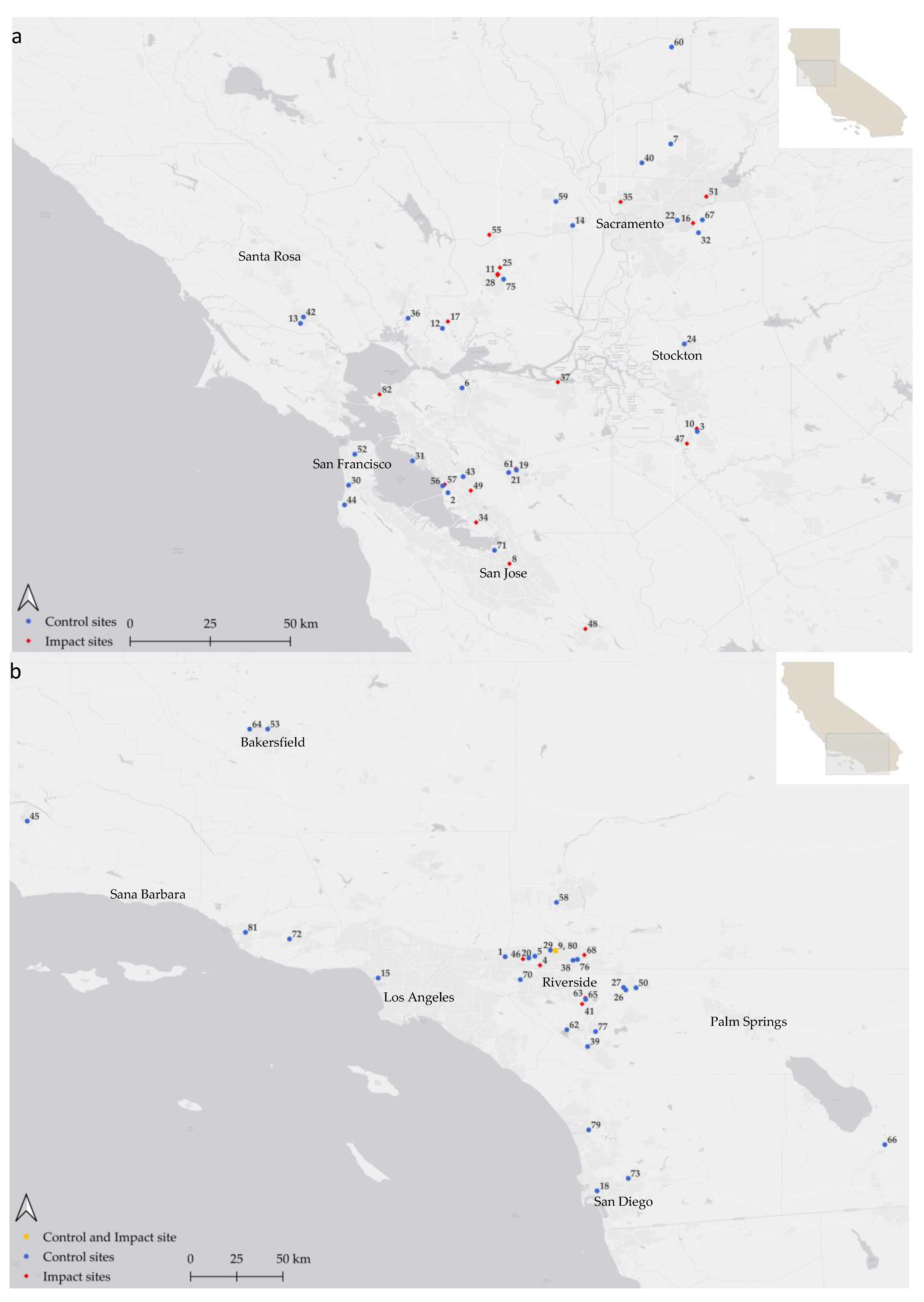
Figure 2.
GLP Warehouse Project site on 12 February 2020 (top) and 18 February 2022 (bottom).
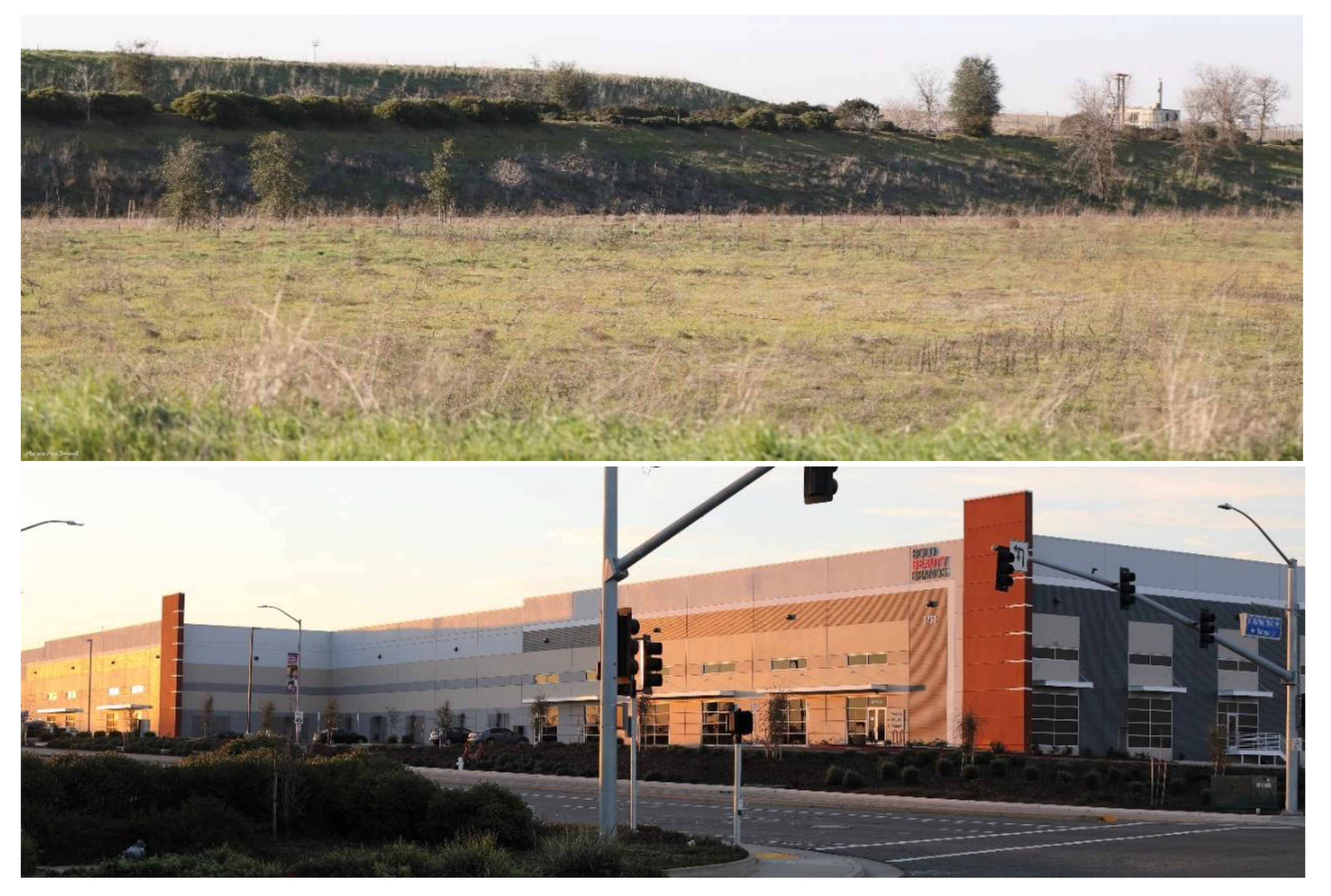
Figure 3.
First Industrial Warehouse Project site on 28 February 2020 (top) and 5 February 2023 (bottom).
Figure 3.
First Industrial Warehouse Project site on 28 February 2020 (top) and 5 February 2023 (bottom).
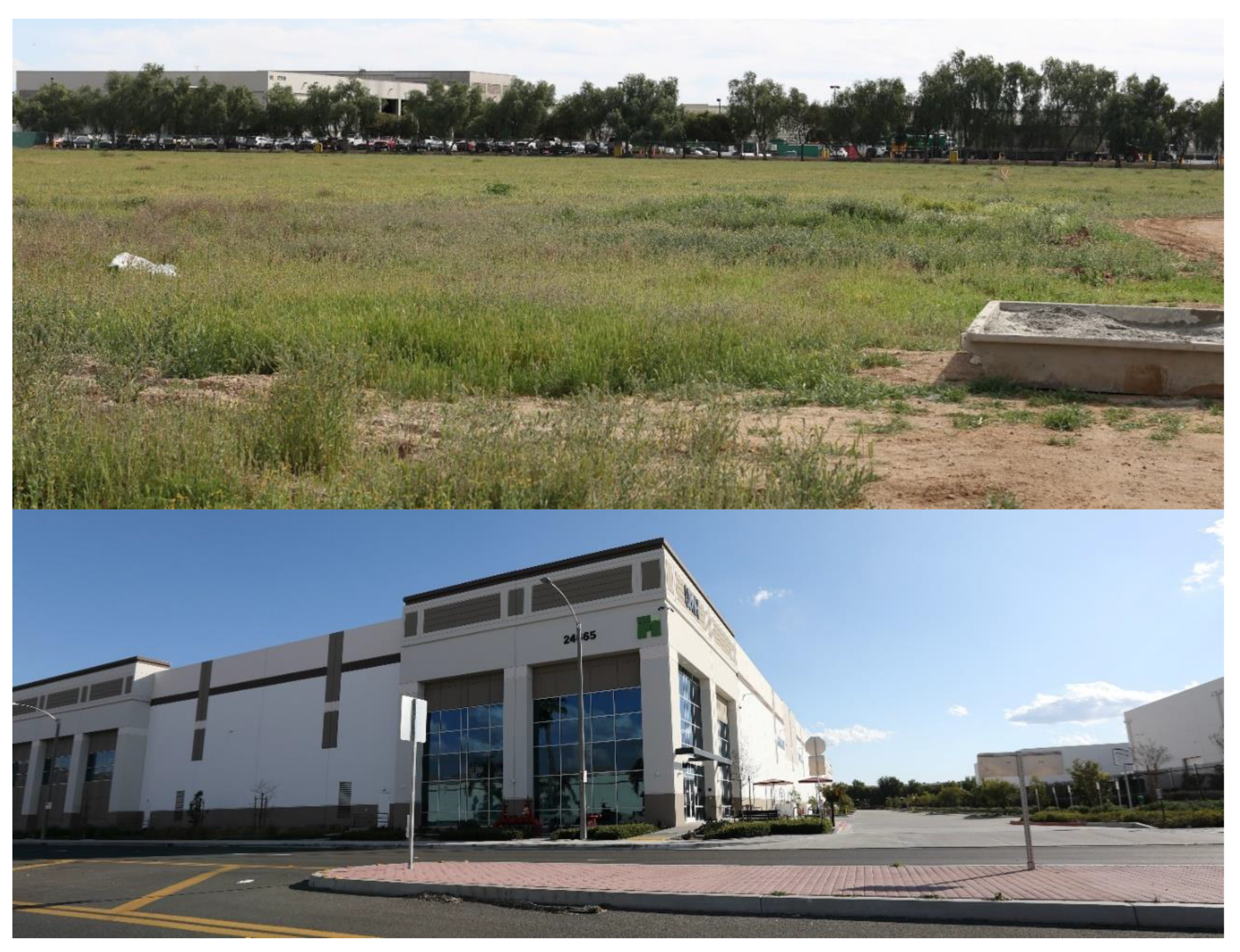
Figure 4.
Winters Highlands residential project site on 18 May 2004 (top) and 11 June 2021 (bottom). A pair of burrowing owls are visible in the foreground, center-left aspect of the top photo.
Figure 4.
Winters Highlands residential project site on 18 May 2004 (top) and 11 June 2021 (bottom). A pair of burrowing owls are visible in the foreground, center-left aspect of the top photo.
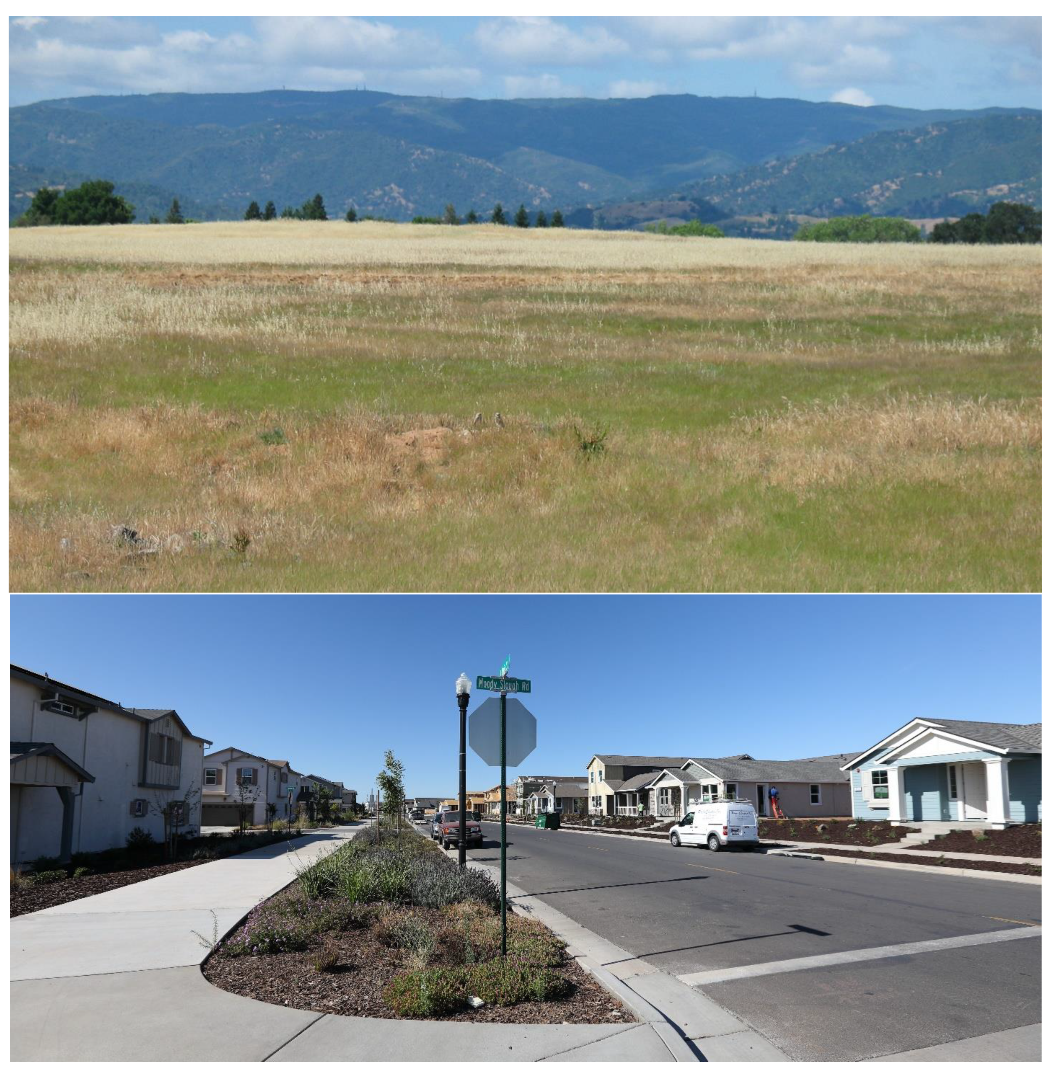
Figure 5.
Western meadowlark on the Mango Avenue Warehouse project site in Fontana, despite the ground disturbance caused by human activities.
Figure 5.
Western meadowlark on the Mango Avenue Warehouse project site in Fontana, despite the ground disturbance caused by human activities.
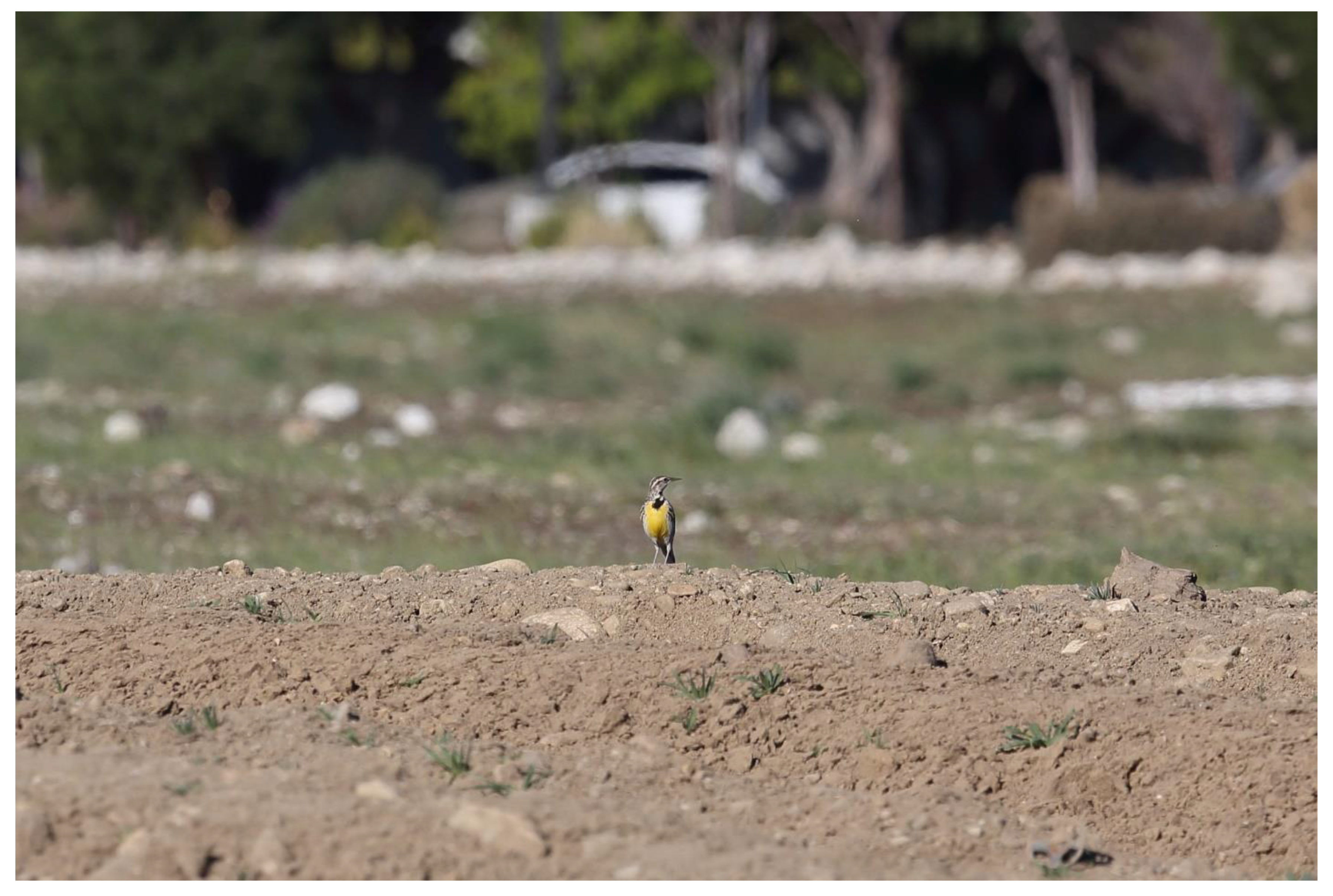
Figure 6.
Despite the dominant tree cover of non-native blue gum eucalyptus (Eucalyptus globulus) on Mount Sutro Open Space Reserve, which was one of our control sites, Pacific wren continued to thrive on site, along with numerous other species of vertebrate wildlife.
Figure 6.
Despite the dominant tree cover of non-native blue gum eucalyptus (Eucalyptus globulus) on Mount Sutro Open Space Reserve, which was one of our control sites, Pacific wren continued to thrive on site, along with numerous other species of vertebrate wildlife.
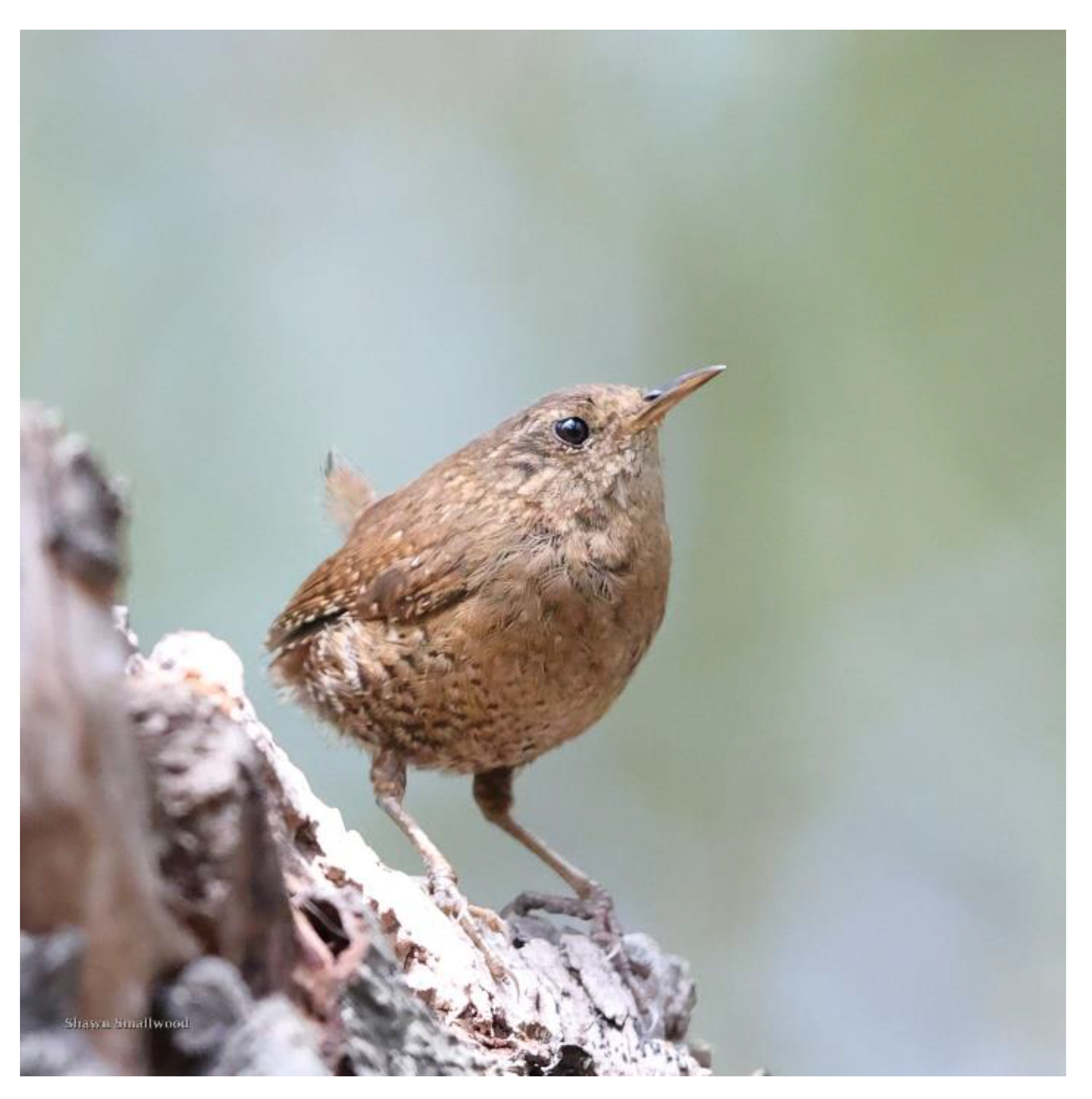
Figure 7.
Feral house cat on the Alviso Hotel Project site in San Jose – a site that had not been developed during our study and which we therefore treated as a control site.
Figure 7.
Feral house cat on the Alviso Hotel Project site in San Jose – a site that had not been developed during our study and which we therefore treated as a control site.
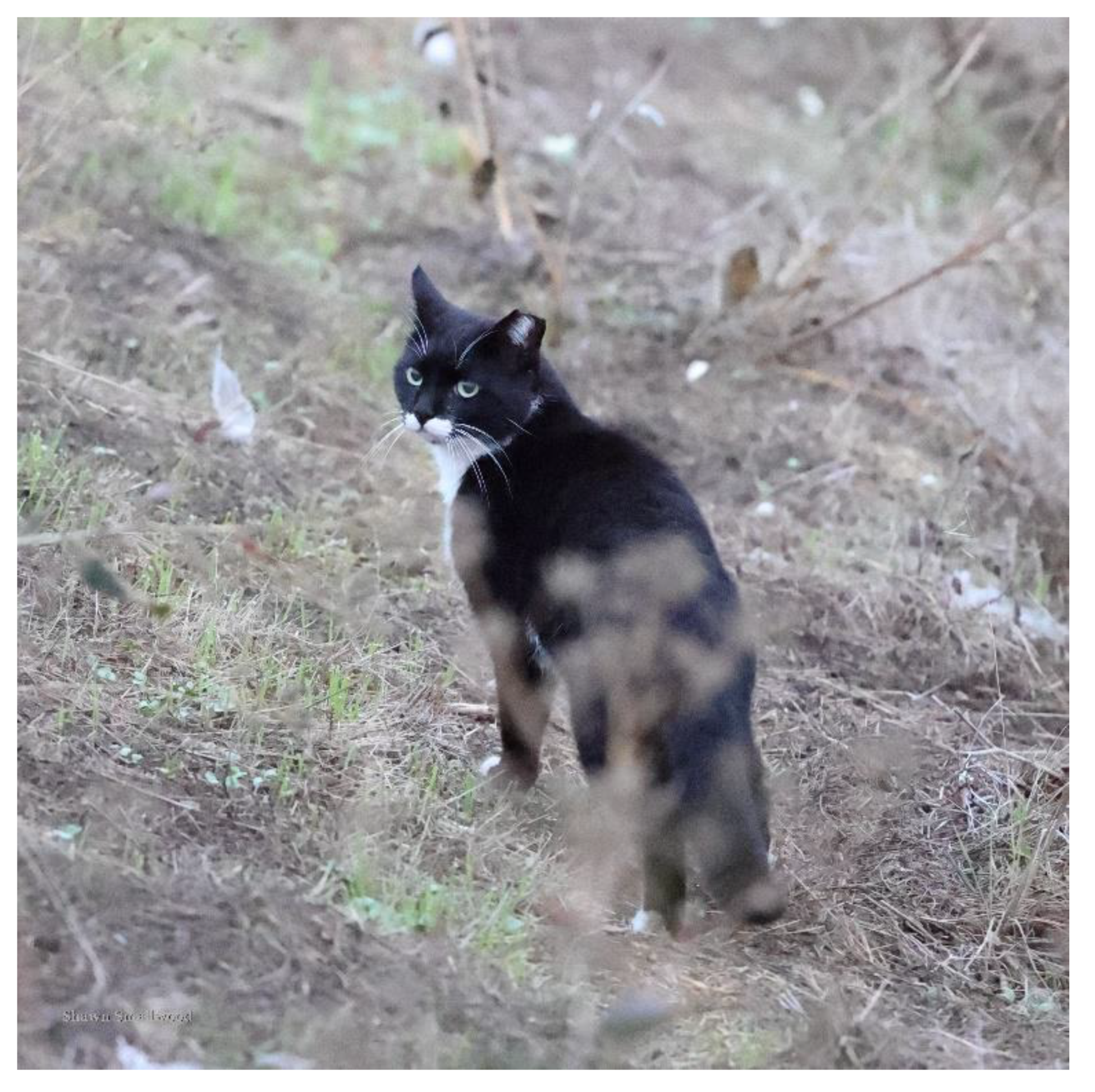
Figure 8.
Mean and 95% confidence intervals (CI) of model-predicted number of vertebrate wildlife species detected by minute into the reconnaissance survey and extended to 5 hours (a) and only 1 hour (b), where for each survey the model fit to the cumulative number of species detected, Y, was of the form: , where X represents minutes into the survey, and a, b, and c were best-fit coefficients. The coefficient of determination, r2, averaged among the models fit to the data.
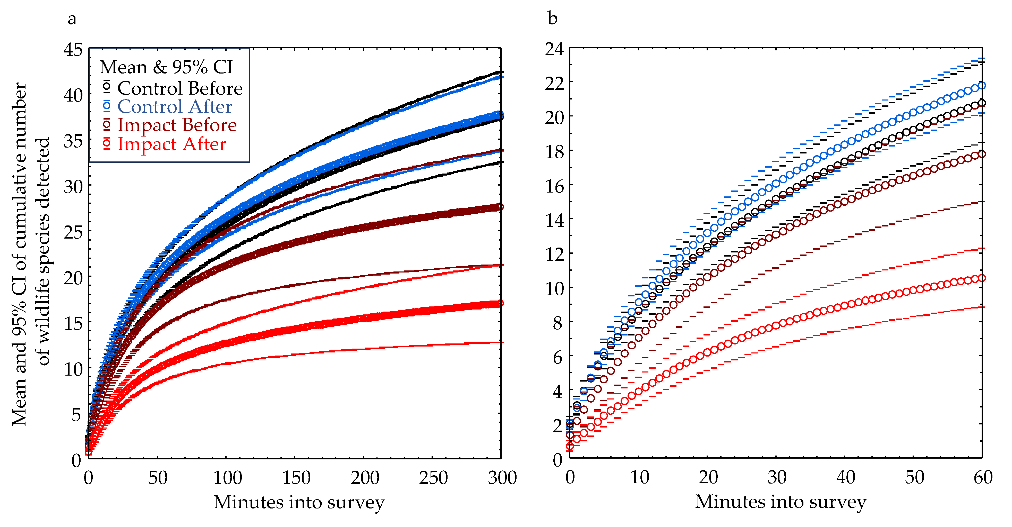
Figure 9.
A savannah sparrow on the Operon HKI Project site in Perris on 21 November 2021, which was the date of the first survey in the before phase. Twice as many savannah sparrows were counted in the second survey at this site, which was not developed. Where projects were developed, development impacts reduced savannah sparrow counts by 63% on average.
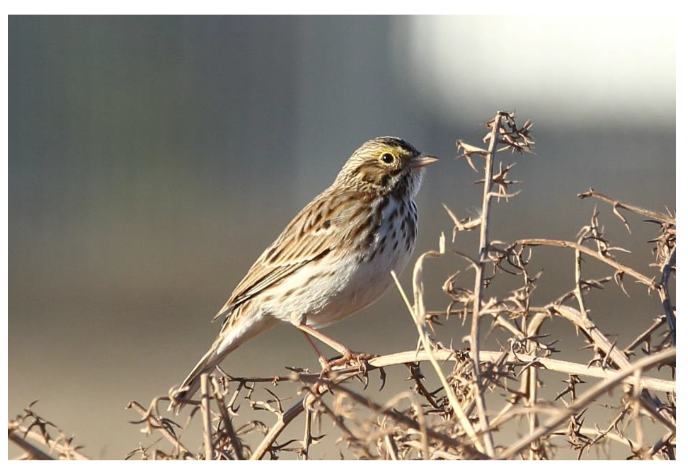
Figure 10.
BACI tests revealed that development reduced the number of species detected by 48% (a) and the number of species detected within the bounds of the study site by 66% (b). The red dashed arrow points to the expected value had no development impact occurred.
Figure 10.
BACI tests revealed that development reduced the number of species detected by 48% (a) and the number of species detected within the bounds of the study site by 66% (b). The red dashed arrow points to the expected value had no development impact occurred.
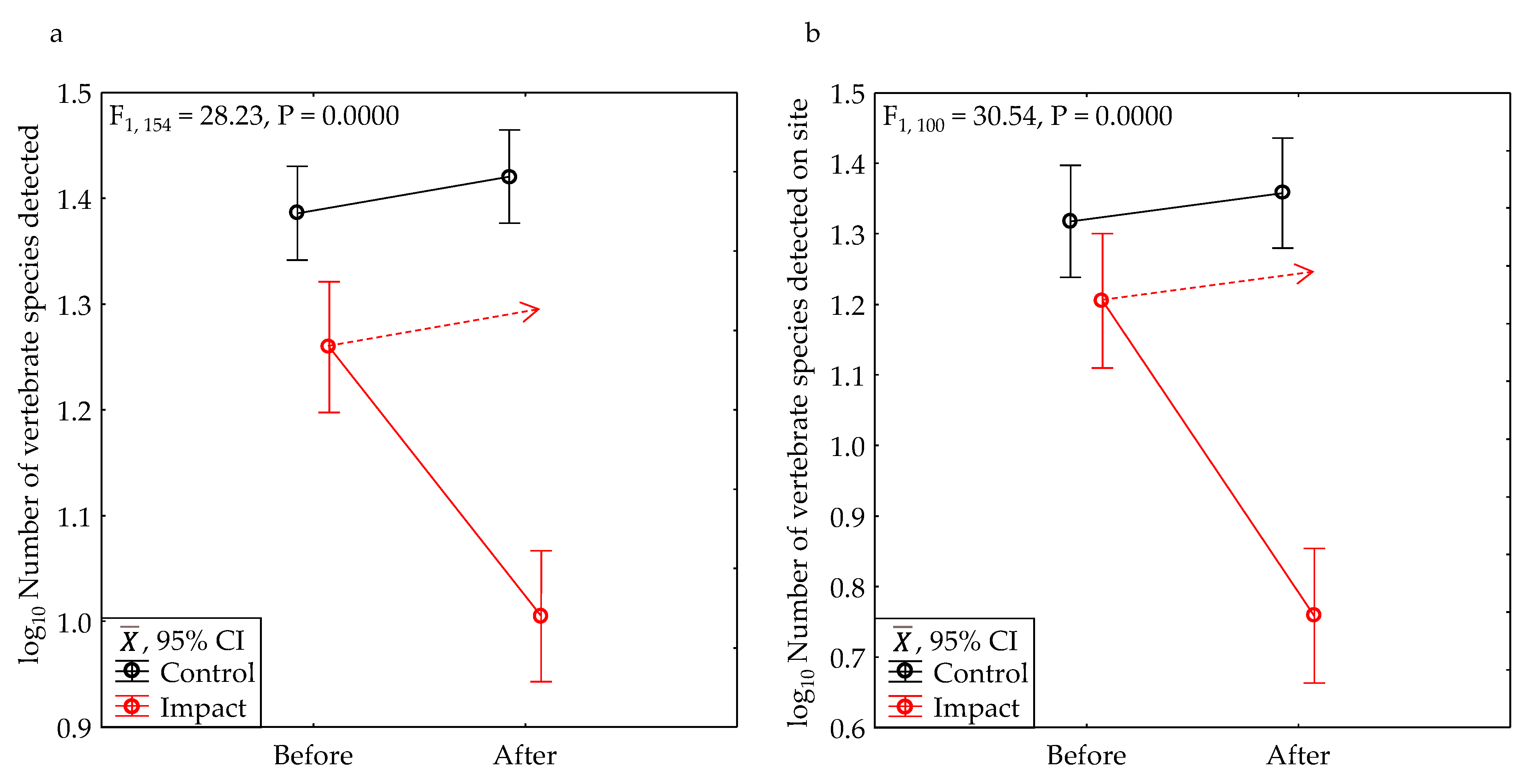
Figure 11.
BACI tests revealed that development reduced the counts of observed animals by 90% (a) and the counts of observed animals within the bounds of the study site by 91% (b). The red dashed arrow points to the expected value had no development impact occurred.
Figure 11.
BACI tests revealed that development reduced the counts of observed animals by 90% (a) and the counts of observed animals within the bounds of the study site by 91% (b). The red dashed arrow points to the expected value had no development impact occurred.
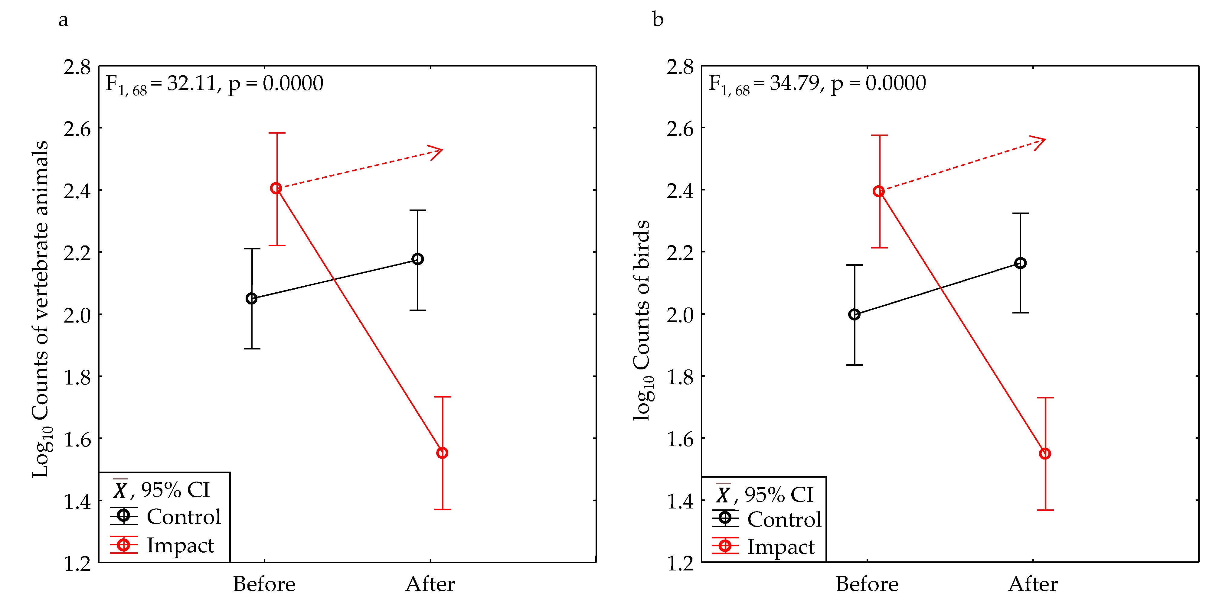
Figure 12.
BACI tests revealed that development reduced the number of special-status species detected by 49% (a) and the number of special-status species detected within the bounds of the study site by 58% (b). The red dashed arrow points to the expected value had no development impact occurred.
Figure 12.
BACI tests revealed that development reduced the number of special-status species detected by 49% (a) and the number of special-status species detected within the bounds of the study site by 58% (b). The red dashed arrow points to the expected value had no development impact occurred.
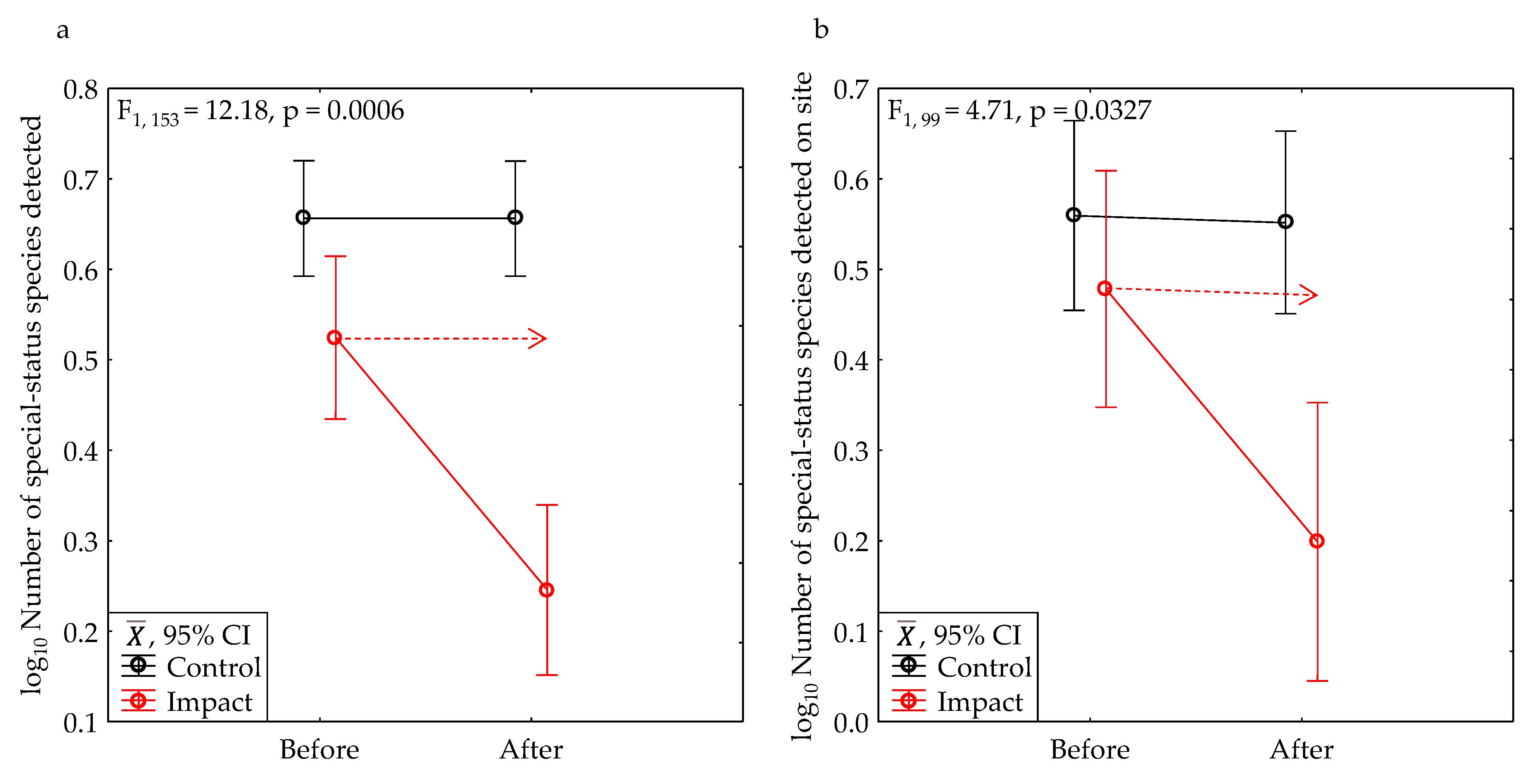
Figure 13.
A BACI test revealed that development reduced the mean model-predicted number of species detected after one hour of survey by 37% (a), and the number of uniquely detected species at a site in one phase relative to the species detected in the other phase declined by 74% (b). The red dashed arrow points to the expected value had no development impact occurred.
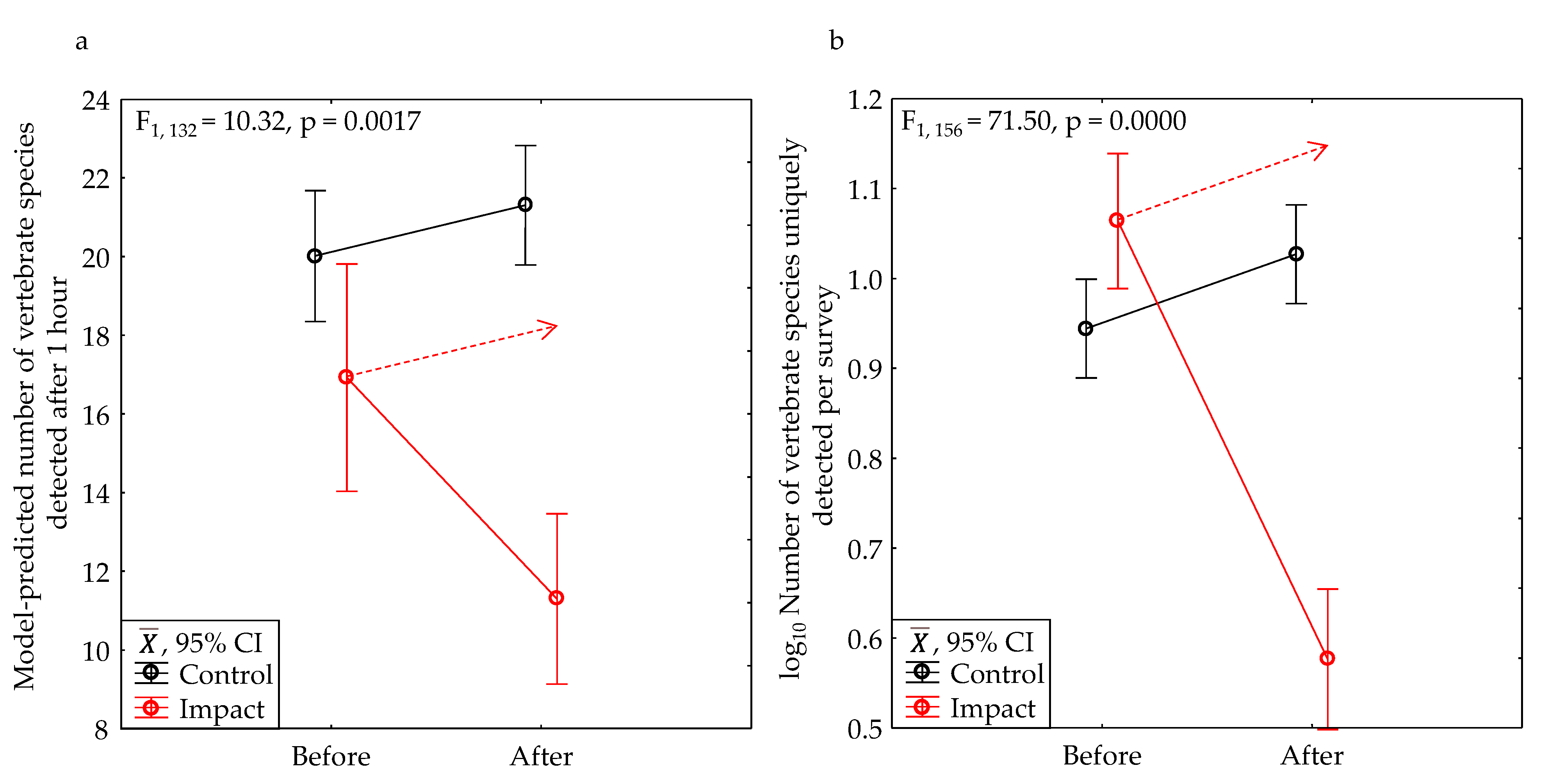
Figure 14.
ANOVA residuals of (a) number of vertebrate species detected and of (b) model-predicted number of vertebrate species detected at one hour regressed on survey duration (minutes).
Figure 14.
ANOVA residuals of (a) number of vertebrate species detected and of (b) model-predicted number of vertebrate species detected at one hour regressed on survey duration (minutes).
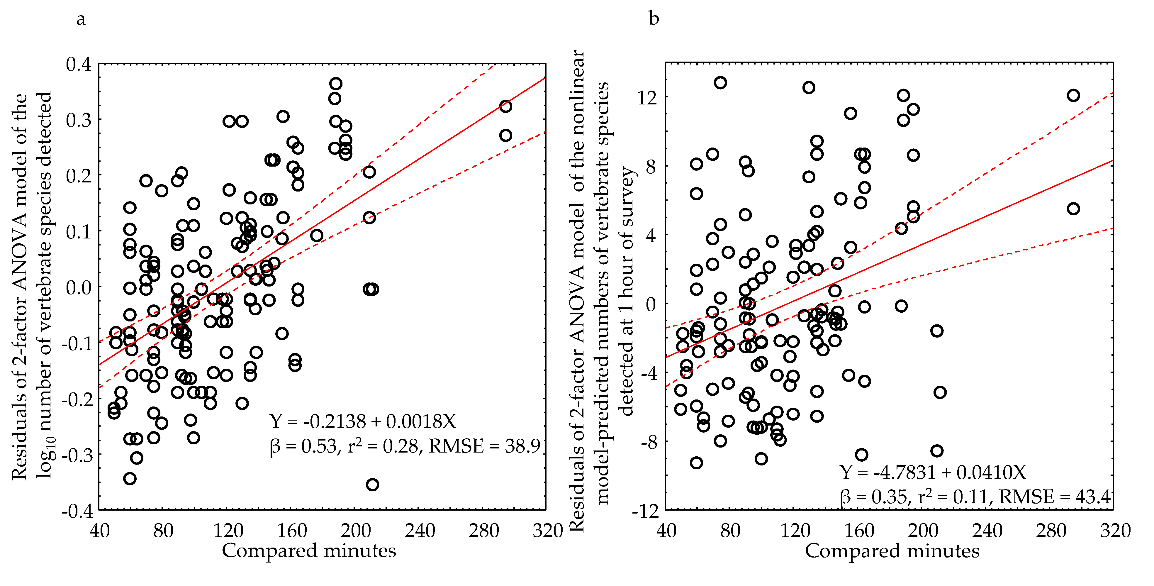
Figure 15.
ANOVA residuals of model-predicted number of vertebrate species detected at one hour compared by (a) whether the project site was situated in open space or as infill or redevelopment within developed areas, and by (b) percentage of the project boundary adjacent to open space.
Figure 15.
ANOVA residuals of model-predicted number of vertebrate species detected at one hour compared by (a) whether the project site was situated in open space or as infill or redevelopment within developed areas, and by (b) percentage of the project boundary adjacent to open space.
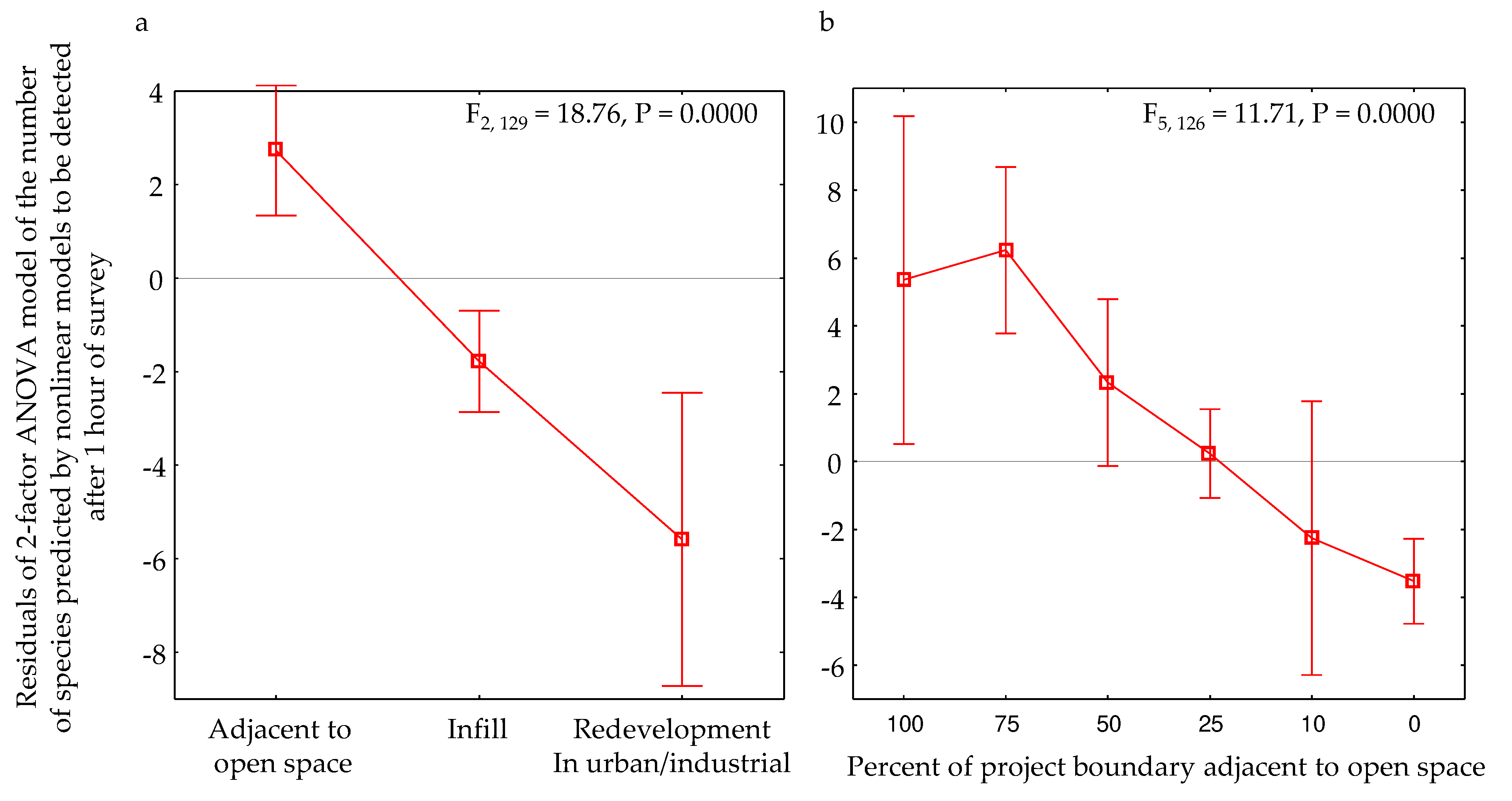
Figure 16.
A Botta’s pocket gopher peers from its burrow system on the Brokaw Campus project site in San Jose on 16 November 2018. This and any other pocket gopher stood no chance of survival following the development of the project, and no evidence of this species was evident during the second survey of 30 October 2021.
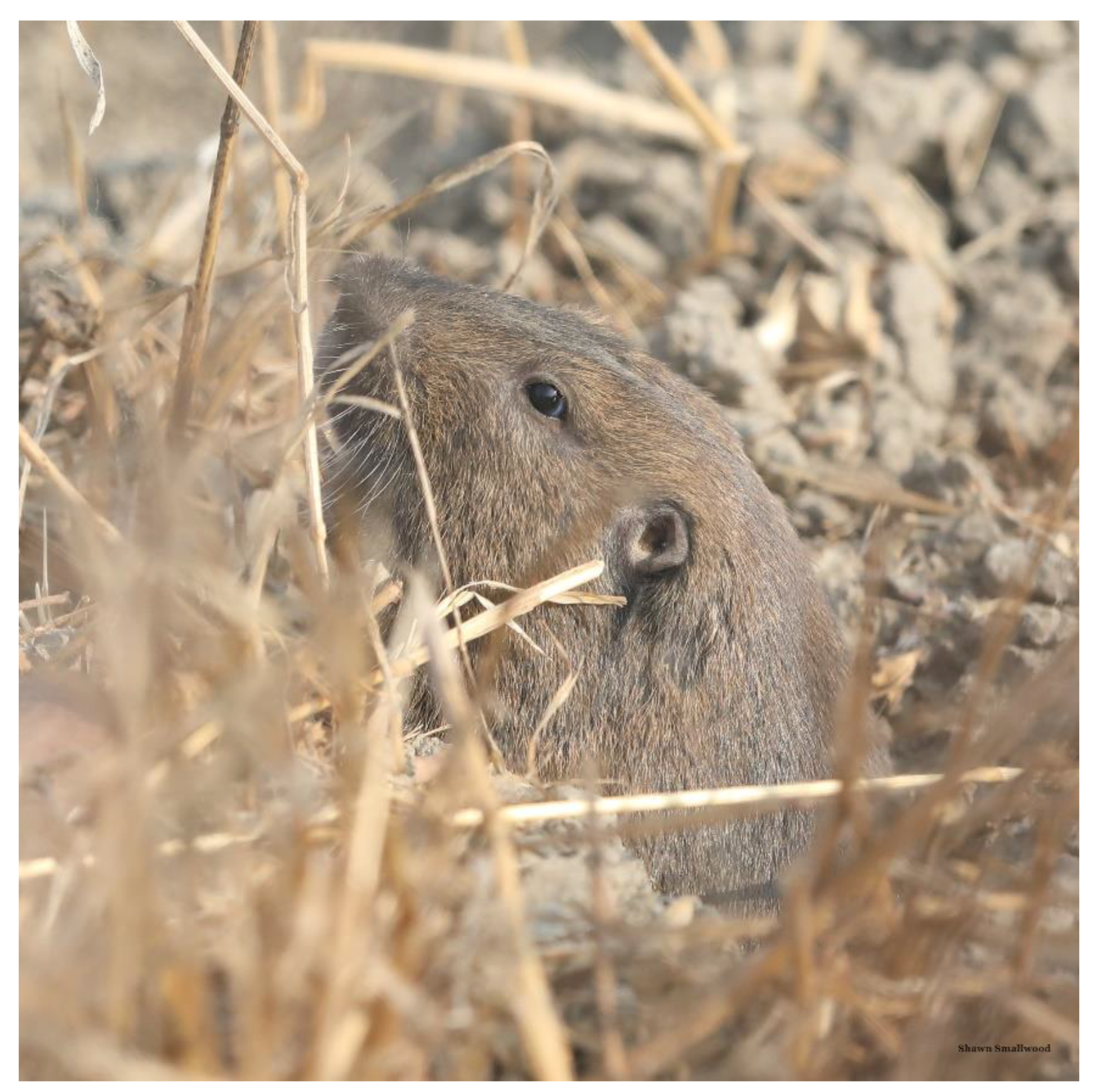
Figure 17.
Although loggerhead shrike was detected on 23 June 2019 at the Monte Vista Warehouse Project site in Vacaville, it was not detected in the follow-up survey on 16 June 2021 after the project was built.
Figure 17.
Although loggerhead shrike was detected on 23 June 2019 at the Monte Vista Warehouse Project site in Vacaville, it was not detected in the follow-up survey on 16 June 2021 after the project was built.
Table 1.
Summary of survey and site attributes of 78 project sites we surveyed in California, 2002-2023.
Table 1.
Summary of survey and site attributes of 78 project sites we surveyed in California, 2002-2023.
| Metric | CB (n = 52) | CA (n = 52) | IB (n = 26) | IA (n= 26) | ||||
|---|---|---|---|---|---|---|---|---|
| SD | SD | SD | SD | |||||
| Size of project site (Hectares) | 131 | 310 | 16.25 | 30.22 | ||||
| Elevation (m) | 175 | 214 | 138 | 243 | ||||
| Northing (m) | 3994623 | 241749 | 4088256 | 213973 | ||||
| Urban setting | 0.55 | 0.61 | 0.77 | 0.51 | ||||
| Connectivity (%) | 35.0 | 30.8 | 35.0 | 30.8 | 17.3 | 19.7 | 15.4 | 17.4 |
| Project site disturbance | 4.12 | 2.70 | 4.13 | 2.70 | 5.20 | 2.69 | 10.58 | 1.65 |
| Rating of suppressive actions | 1.24 | 1.92 | 1.51 | 2.24 | 2.58 | 2.47 | 5.50 | 1.63 |
| Survey duration (minutes) | 128 | 47 | 125 | 46 | 96 | 38 | 96 | 38 |
| Years since first survey | 2.7 | 3.9 | 4.0 | 4.2 | ||||
| Start time difference (minutes) | -3.6 | 38.0 | -2.9 | 34.4 | ||||
Table 2.
Mean and standard deviation of the number of species detected and the number of animals counted in reconnaissance surveys, and the number of sites (N) within the BACI experimental treatment levels control-before (CB), control-after (CA), impact-before (IB), and impact-after (IA), where impact sites were those at which a proposed projects had been developed prior to the survey that was completed in the after phase of the study. All project sites were in California. Unique species per survey refers to the number of uniquely detected species at a site in one phase relative to the species detected in the other phase.
| Metric | CB | CA | IB | IA | Effect | ||||||||
|---|---|---|---|---|---|---|---|---|---|---|---|---|---|
| SD | N | SD | N | SD | N | SD | N | ||||||
| Number of species | |||||||||||||
| All vertebrates | 26.4 | 11.1 | 51 | 28.2 | 10.7 | 51 | 19.1 | 5.9 | 26 | 10.7 | 3.7 | 26 | -48 |
| Onsite vertebrates | 22.8 | 12.9 | 30 | 25.5 | 12.6 | 30 | 17.4 | 6.6 | 20 | 6.6 | 3.3 | 20 | -66 |
| All birds | 23.5 | 9.6 | 51 | 25.2 | 9.4 | 51 | 17.6 | 5.9 | 26 | 10.3 | 3.6 | 26 | -45 |
| Onsite birds | 19.9 | 11.3 | 30 | 22.5 | 11.1 | 30 | 16.0 | 6.4 | 20 | 6.5 | 3.3 | 20 | -64 |
| All mammals | 2.5 | 2.3 | 51 | 2.4 | 1.9 | 51 | 1.3 | 0.9 | 26 | 0.3 | 0.6 | 26 | -79 |
| Onsite mammals | 2.5 | 2.4 | 30 | 2.3 | 2.0 | 30 | 1.3 | 1.0 | 20 | 0.1 | 0.3 | 20 | -92 |
| All herps | 0.4 | 0.7 | 51 | 0.5 | 0.8 | 51 | 0.2 | 0.4 | 26 | 0.1 | 0.3 | 26 | -47 |
| Onsite herps | 0.5 | 0.9 | 27 | 0.6 | 0.7 | 27 | 0.1 | 0.3 | 20 | 0.0 | 0.0 | 20 | -100 |
| All non-birds | 2.9 | 2.6 | 51 | 3.0 | 2.1 | 51 | 1.5 | 1.0 | 26 | 0.4 | 0.8 | 26 | -75 |
| Onsite non-birds | 2.9 | 2.9 | 30 | 2.8 | 2.3 | 30 | 1.4 | 1.0 | 20 | 0.1 | 0.2 | 20 | -96 |
| All special-status species | 5.2 | 2.8 | 51 | 4.9 | 2.3 | 51 | 3.7 | 2.1 | 26 | 1.8 | 1.0 | 25 | -49 |
| Onsite special-status species | 4.3 | 3.1 | 30 | 4.3 | 2.5 | 30 | 3.0 | 1.8 | 20 | 1.3 | 1.3 | 19 | -58 |
| Model-predicted at 1 hour | 20.0 | 6.4 | 42 | 21.3 | 5.2 | 51 | 16.9 | 4.5 | 14 | 11.3 | 4.8 | 25 | -37 |
| Unique species per survey | 9.9 | 5.2 | 51 | 11.6 | 4.9 | 51 | 12.6 | 4.8 | 27 | 3.9 | 2.2 | 27 | -74 |
| Animals counted | |||||||||||||
| All vertebrates | 155.4 | 117.0 | 19 | 187.2 | 157.4 | 19 | 358.7 | 259.0 | 15 | 42.9 | 23.7 | 15 | -90 |
| Onsite vertebrates | 107.7 | 144.3 | 14 | 99.0 | 80.9 | 14 | 335.4 | 284.4 | 14 | 34.9 | 18.2 | 14 | -89 |
| All birds | 135.6 | 102.6 | 19 | 183.3 | 154.3 | 19 | 354.0 | 255.3 | 15 | 42.5 | 23.5 | 15 | -91 |
| Onsite birds | 98.6 | 130.4 | 14 | 96.7 | 80.4 | 14 | 330.5 | 280.3 | 14 | 34.8 | 18.1 | 14 | -89 |
| All special-status species | 30.9 | 67.5 | 19 | 17.3 | 22.2 | 19 | 31.8 | 51.0 | 15 | 5.4 | 6.6 | 14 | -70 |
| Onsite special-status species | 11.8 | 16.0 | 14 | 9.9 | 12.5 | 14 | 35.1 | 54.1 | 13 | 5.3 | 7.4 | 12 | -82 |
Table 3.
Before-after, control-impact (BACI) comparisons of log10 number of vertebrate species detected and log10 number of animals counted in reconnaissance surveys at sites of proposed projects in California, where the CI × BA interaction effect is the principal effect of interest, but tests for main effects are also reported. Also reported are determinations of whether the data were normally distributed based on visual examination of normal probability plots, the p-value of Hartley’s F-max test for homogeneity of variance, and statistical power (1–β, where β is the probability of a Type II error) estimated for the interaction effect. Unique species per survey refers to the number of uniquely detected species at a site in one phase relative to the species detected in the other phase.
| Metric | Normally distributed? |
Hartley's F-max P-value |
Control-Impact main effect |
Before-After main effect |
CI × BA interaction effect |
||||
|---|---|---|---|---|---|---|---|---|---|
| F | P | F | P | F | P | 1–β | |||
| Number of species | |||||||||
| All vertebrates | Yes | 0.6161 | 99.34 | 0.0000 | 16.31 | 0.0001 | 28.23 | 0.0000 | 1.00 |
| Onsite vertebrates | Yes | 0.7228 | 65.44 | 0.0000 | 21.31 | 0.0000 | 30.54 | 0.0000 | 1.00 |
| All birds | Yes | 0.7747 | 84.00 | 0.0000 | 12.52 | 0.0005 | 23.90 | 0.0000 | 1.00 |
| Onsite birds | Yes | 0.6205 | 49.67 | 0.0000 | 15.93 | 0.0001 | 26.42 | 0.0000 | 1.00 |
| All mammals | Yes | 0.0600 | 8.52 | 0.0043 | 0.60 | 0.4408 | 0.03 | 0.8560 | 0.05 |
| Onsite mammals | Yes | 0.1827 | 5.78 | 0.0192 | 1.20 | 0.2783 | 0.60 | 0.4402 | 0.12 |
| All herps | Yes | 1.0000 | 3.07 | 0.0888 | 0.01 | 0.9104 | 0.01 | 0.9104 | 0.05 |
| Onsite herps | |||||||||
| All non-birds | Yes | 0.0622 | 14.50 | 0.0002 | 1.19 | 0.2770 | 0.56 | 0.4576 | 0.11 |
| Onsite non-birds | Yes | 0.0837 | 4.24 | 0.0436 | 0.71 | 0.4029 | 0.47 | 0.4947 | 0.10 |
| All special-status species | Yes | 0.6230 | 46.00 | 0.0000 | 12.18 | 0.0006 | 12.18 | 0.0006 | 0.93 |
| Onsite special-status species | Yes | 0.2806 | 12.05 | 0.0008 | 5.26 | 0.0242 | 4.71 | 0.0327 | 0.57 |
| Model-predicted at 1 hour | Yes | 0.2336 | 37.04 | 0.0000 | 4.06 | 0.0459 | 10.32 | 0.0017 | 0.89 |
| Unique species per survey | Yes | 0.7910 | 24.05 | 0.0000 | 36.01 | 0.0000 | 71.50 | 0.0000 | 1.00 |
| Animals counted | |||||||||
| All vertebrates | Yes | 0.2890 | 2.44 | 0.1235 | 17.80 | 0.0001 | 32.11 | 0.0000 | 1.00 |
| Onsite vertebrates | snaky | 0.0035 | 0.02 | 0.8842 | 7.40 | 0.0088 | 11.77 | 0.0012 | 0.92 |
| All birds | Yes | 0.2916 | 1.62 | 0.2076 | 15.63 | 0.0002 | 34.79 | 0.0000 | 1.00 |
| Onsite birds | Yes | 0.0040 | 0.00 | 0.9964 | 6.68 | 0.0126 | 11.86 | 0.0011 | 0.92 |
| All special-status species | Yes | 0.8945 | 1.96 | 0.1672 | 10.11 | 0.0023 | 4.76 | 0.0331 | 0.57 |
| Onsite special-status species | Yes | 0.8629 | 0.84 | 0.3647 | 9.87 | 0.0030 | 6.15 | 0.0171 | 0.68 |
Table 5.
Mean number of species detected per survey in each identified species’ group among the surveys in the experimental treatment groups of control-before, control-after, impact-before and impact-after. Measures of percentage effect of development appear in the right column.
Table 5.
Mean number of species detected per survey in each identified species’ group among the surveys in the experimental treatment groups of control-before, control-after, impact-before and impact-after. Measures of percentage effect of development appear in the right column.
| Group | Control (n = 52) | Impact (n = 26) | Effect (%) | ||
|---|---|---|---|---|---|
| Before | After | Before | After | ||
| Birds | 23.1 | 25.73 | 17.73 | 10.19 | -48 |
| Mammals | 2.52 | 2.42 | 1.38 | 0.19 | -86 |
| Reptiles | 0.33 | 0.33 | 0.08 | 0.08 | 0 |
| Amphibians | 0.06 | 0.4 | 0.04 | 0 | -100 |
| Special status species | 5.11 | 4.88 | 3.69 | 1.81 | -49 |
| Non-native birds | 1.98 | 2.37 | 2.69 | 1.81 | -44 |
| Synanthropic birds | 7.19 | 7.67 | 7.42 | 5.73 | -28 |
| Raptors | 2.77 | 2.61 | 2.58 | 1.15 | -53 |
| Grassland birds | 1.9 | 1.81 | 1.5 | 0.36 | -75 |
Disclaimer/Publisher’s Note: The statements, opinions and data contained in all publications are solely those of the individual author(s) and contributor(s) and not of MDPI and/or the editor(s). MDPI and/or the editor(s) disclaim responsibility for any injury to people or property resulting from any ideas, methods, instructions or products referred to in the content. |
© 2023 by the authors. Licensee MDPI, Basel, Switzerland. This article is an open access article distributed under the terms and conditions of the Creative Commons Attribution (CC BY) license (https://creativecommons.org/licenses/by/4.0/).
Copyright: This open access article is published under a Creative Commons CC BY 4.0 license, which permit the free download, distribution, and reuse, provided that the author and preprint are cited in any reuse.


