Submitted:
27 July 2023
Posted:
28 July 2023
You are already at the latest version
Abstract
The goal of this paper is the performance evaluation of a deep learning approach when deployed in fifth-generation (5G) millimeter wave (mmWave) multicellular networks. To this end, the optimum beamforming configuration is defined by two neural networks (NNs) that are properly trained, according to mean square error (MSE) minimization. The first network has as input the requested spectral efficiency (SE) per active sector, while the second network the corresponding energy efficiency (EE). Hence, channel and power variations can now be taken into consideration during adaptive beamforming. The performance of the proposed approach is evaluated with the help of a developed system level simulator via extensive Monte Carlo simulations. According to the presented results, machine learning (ML)-adaptive beamforming can significantly improve EE compared to the standard non-ML framework. Although this improvement comes at the cost of increased blocking probability (BP) and radiating elements (REs) for high data rate services, the corresponding increase ratios are significantly reduced compared to the EE improvement ratio. In particular, considering 21.6 Mbps per active user and ML adaptive beamforming, then EE can reach up to 5.3 Mbps/W, which is significantly improved compared to the non-ML case (0.9 Mbps/W). In this context, BP does not exceed 2.6%, which is slightly worse compared to 1.7% in the standard non-ML case. Moreover, approximately 20% additional REs are required, with respect to the non-ML framework.
Keywords:
5G
; mmWave
; Massive MIMO
; Machine Learning
; Adaptive Beamforming
; System Level Simulations.
1. Introduction
The full deployment of fifth-generation (5G) broadband wireless cellular networks has enabled the transition towards advanced features and applications, such as enhanced mobile broadband (eMBB), ultra-reliable low latency communications (URLLC) as well as massive machine type communications (mMTC) [1,2]. To this end, various novel tech-nologies have been introduced in the physical layer, such as millimeter-wave (mmWave) transmission [3], non-orthogonal multiple access (NOMA) [4] as well as massive multiple input multiple output (m-MIMO) configurations [5]. Moreover, as the discussions on the next generation of wireless networks (sixth generation, 6G) have already started taking place [6], network densification is leveraged as an efficient way to provide seamless connectivity to a vast number of mobile devices. In this context, the single link concept (i.e., base station-BS to mobile station-MS) is replaced by various potential links from access points (APs) and relay nodes.
As may be seen from the preceding, in next generation wireless networks a significantly large number of antennas will be deployed per AP. Hence, appropriate beamforming algorithms should be configured that not only ensure uninterrupted connectivity but also minimize interference levels. In this paper, we deal with a computationally efficient adaptive beamforming technique in multicellular mmWave m-MIMO orientations. In this case, the goal is to improve various key performance indicators (KPIs), such as energy efficiency (EE) and spectral efficiency (SE). In general, adaptive beamforming in 5G orientations has attracted scientific research interest over the last years. In this context, in [7] the performance of various precoding schemes is evaluated, with emphasis in hybrid beamforming, which is a challenging beamforming approach that is based on the use of fewer active radio-frequency (RF) chains compared to the total number of antennas. According to the presented results, hybrid precoding methods can improve sum rate and SE. In particular, one of the main effective hybrid precoder proposed in the literature of m-MIMO beamforming schemes is phased-zero-forcing (PZF), which improves signal-to-noise ratio (SNR) and SE. However, [8] manifests that PZF beamforming needs further improvement in densely-deployed networks. In the same context of m-MIMO beamforming, the provided simulations in [9] suggest higher number of parallel data streams per user in a mmWave system to achieve higher order throughputs. Interestingly enough, it has been demonstrated that the need for active antenna elements decreases with the number of parallel data streams. In [10], the concept of ultra-dense cell-free m-MIMO systems for sustainable 6G wireless communications is introduced. The key findings of the work conclude that the support of high data rates requires a holistic network redesign to maximize EE (dense deployment, green design, etc.). In a similar cell-free m-MIMO system, [11] proposes an optimum beamforming scheme which outperforms zero-forcing and conjugate beamforming. Even though the former work can achieve beamforming and power control, it increases significantly the system’s complexity. In [12], the performance of the least mean square (LMS) algorithm is investigated, in the context of 5G-MIMO configurations. To this end, several optimization algorithms are evaluated under various parameters (i.e., antenna elements, antenna spacing, etc.).
The coexistence of various novel technologies in the physical layer of the next generation broadband wireless networks as it was previously mentioned, along with increased user traffic and mobility patterns, create a multiparameter environment with various constraints. Hence, traditional optimization algorithms on one hand would have to search over multidimensional spaces for potential solutions, and on the other hand optimization process would have to be repeated over regular time intervals (e.g., coherence time). Therefore, latency minimization, which is a key concept in 5G/6G networks would not always be satisfied. Over the last years, machine learning (ML) algorithms have emerged as a promising solution that can deal with a variety of optimization problems. In general, ML algorithms can be classified into three major categories [13,14,15]: supervised learning (SL) where training is based on well-known datasets, unsupervised learning, where there is no data pattern, as well as reinforcement learning (RL). In the latter case, a mobile agent interacts with the environment to define the best possible action per case.
In the ML framework, a survey of the most important approaches categorized per m-MIMO application (i.e., channel estimation, signal detection, hybrid beamforming, coexistence with NOMA, etc.) is provided in [16]. In [17] a novel deep reinforcement learning (DRL) based coordinated beamforming scheme has been considered, where a single MS can be served by multiple BSs. In this context, the goal is to derive suboptimal beamforming vectors at BSs out of possible beamforming codebook candidates. The beamforming vectors are chosen according to sum rate maximization. In [18], the concept of federated learning (FL) in m-MIMO configurations is introduced to optimize various metrics, such as MS assignments and transmission powers. To this end, ML-aided resource optimization is performed in a decentralized way, in discrete time intervals.
In [19], a SL approach is considered for user positioning that can outperform other ML schemes such as k-nearest neighbors (k-NN) algorithm and support vector machines (SVM). In [20], a deep learning (DL) approach is presented to simplify the process of estimating beamforming weights. According to the presented results, the proposed approach can significantly reduce overall complexity in weight estimation. In [21], hybrid beamforming is used for EE maximization. In the same context, a low-complexity method that is based on adaptive cross-entropy (ACE)-based optimization with low-bit phase shifters was proposed in order to handle the sum rate maximization problem. In [22], the authors present an approach based on convolutional neural network (CNN) structure, namely WBPNet, to realize adaptive time-domain wideband beamforming without delay structures under insufficient snapshots. In [23], the authors evaluate the performance of an adaptive beamforming approach in 5G multicellular mmWave configurations with the help of a k-NN SL method that selects the appropriate beamforming configuration based on the requested SE in an active sector. According to the presented results, this approach provides similar SE and EE levels when compared to the conventional non-ML approach, at the cost however of increased BP.
The goal of the study presented in this paper is to extend the work in [23] and investigate the performance of a DL approach, when deployed in 5G multicellular wireless orientations. To this end, the algorithm is trained with the help of a predefined number of samples to define the optimum positions of the generated beams. A key novelty of the proposed approach is that two NNs are now considered, one for SE and one for EE maximization. Hence, CSI knowledge can now be exploited during NN training in order to capture channel and power variations. As it will be discussed in the results section, the proposed approach can significantly improve EE for high data rate services compared to the standard non-ML approach, with minimum BP and number of REs increase.
The rest of this paper is organized as follows: In Section 2, the multicellular orienta-tion is described, while the deployed antenna configuration per BS’s sector is described in Section 3. In Section 4, the proposed ML adaptive beamforming framework is analyzed. In Section 5, the overall simulation setup is presented along with simulation results. Finally, concluding remarks are outlined in Section 6.
The following notation is used in the paper. An italic variable a denotes a scalar, whereas boldface lowercase and uppercase variables a and A denote vectors and matrices, respectively. Finally, a calligraphic denotes a set of elements and notation x:y all elements from to x to y with step 1.
2. Multicellular Orientation
We consider a multicellular orientation where MSs enter the network sequentially. At a given state in an arbitrary BS, the MSs follow a specific spatial distribution. According to this distribution the appropriate beamforming configuration (BC) is selected based on the minimization of total downlink transmission power. Hence, the state per BS’s sector is defined by the set {Sb,s,BC(b,s)}, where Sb,s is an 1×180 vector matrix where non-zero entries indicate either the requested SE or EE in the corresponding angles. In the same context, BC(b,s) indicates the BC in the sth sector of the bth BS (1≤s≤3, 1≤b≤B). The overall geometry is depicted in Figure 1, for two tiers of cells around the central cell (19 cells in total). As it can be observed, there are three antenna configurations per BS, located at the boundaries of the hexagonal cell, covering each one an azimuth space of 180o. More details on the deployed antenna configuration per sector will be provided in the following Section.
In 3GPP-channel modeling, a three-model representation of the MIMO channel is considered [24]. To this end, the wireless channel in the 5G air interface for a non-line of sight (NLOS) environment can be modelled as follows:
In this context, the channel coefficient between an arbitrary pair of tx-rx is decomposed to an equivalent number of channel coefficients from N clusters. The channel in each cluster is further decomposed to M subpaths. In (1), Pn represents the power of the nth cluster, Θn,m is a 2×2 matrix with initial phases uniformly distributed in (-π,π) and vector matrices Ftx,n,m/Frx,n,m represent the field pattern of transmitting/receiving antenna element q/u, respectively (1≤q≤Mt, 1≤u≤Mr), for the mth subpath of the nth cluster. Moreover, is the location vector of receive/transmit antenna element u/q, respectively, and λo is the carrier wavelength. Finally, and are the spherical unit vectors.
Corresponding geometry (considering only the x-y plane) is depicted in Figure 2, where ΩBS/ΩMS denote the orientation of the BS/MS antenna array, respectively, defined as the difference between the broadside of the BS/MS array and the absolute North (N) reference direction. Moreover, θBS is the line of sight (LOS) angle of departure (AoD) direction between the BS and MS (with respect to the broadside of the BS array), while θMS is the angle of arrival (AoA) between the BS-MS LOS and the MS broadside. Finally, Δn,m,AoD is the angle offset of the mth subpath with respect to θn,m,AoD and Δn,m,AoA the corresponding offset with respect to θn,m,AoA.
3. Proposed Antenna Design
The employed antenna array configuration scheme of the current work is characterized by low-cost fabrication in an effort to reduce hardware complexity. In particular, the suggested mmWave antenna configuration consists of a 21×21 array of rounded crossed bowtie radiating elements (REs) as shown in Figure 3. In order to achieve a unidirectional radiation pattern with the minimum waste of energy through the back lobe, two ground planes have been located below each RE in a distance of λo/4 and λo/2, respectively, with reference to each rounded bowtie antenna, as shown in the right panel of Figure 3 [25]. It should be noted at this point that the crossed rounded bowtie antennas, used as exciter of the reflector, have been rotated at ±45° to enhance the formulation of an adaptive dual polarized radiation pattern [26], which is a critical property for cellular network communications.
The formulation of all the electromagnetic characteristics of the current array scheme along with a multitude of radiation patterns have been thoroughly presented in our recent published work [23]. Hence, all the produced radiation diagrams as well as technical details about the REs are provided in every detail in the former published work. However, it is necessary to mention that all the antenna field properties have been calculated through the method of moments (MoM) [27], applied in a 3D computational model [28], which incorporates the deleterious effects of mutual coupling among REs. Thus, a realistic analysis of such type of antenna arrays has been carried out.
By using different phases for each RE in conjunction with the appropriate activation of either the entire array or a part of it (subarray), an efficient beamforming technique is adopted. Hence, such arrays increase the levels of manipulation of the radiation pattern. This allows the radiation pattern to be changed not only in terms of the desired direction (azimuth or elevation level) but also in terms of directivity [27]. As a result, a low complexity beamforming technique is suggested, together with an implicit steering mechanism. To this end, 51 different BCs can be formulated, including square and rectangular array configurations. Figure 4 provides an indicative example of the applied BCs, where multiple background colors have been used to distinguish among each other. In conclusion, adopting the proper array configuration necessitates the balancing of three distinct parameters: the number of the activated REs, the desired quality of service (QoS) and the required spatial coverage.
To this end, two representative scenarios explaining the mutual dependence of the aforementioned parameters are presented on the bottom right panel of Figure 4. Assuming that the required spatial coverage is defined between +30° and -30°, the current antenna array can accomplish this requirement with five configuration schemes, as shown in the table on the upper right panel of Figure 4. Supposing that the requested QoS requires an increased directivity, the most appropriate scheme would be 21×3 (63 REs) while a scenario characterized by a low QoS would require the activation of the 3×3 scheme (9 REs). Hence, a scenario with an even reduced required QoS could be facilitated by activating only 1 RE. Consequently, the main priority of the employed algorithm is to detect all the possible configuration schemes which ensure spatial coverage for all MSs of a sector. In turn, the algorithm decides which among them is the most efficient, in terms of power consumption, that accomplishes the demanded QoS.
4. Machine Learning Adaptive Beamforming Framework
In this section, the proposed ML adaptive beamforming framework is presented. A key advantage of the proposed approach is that it considers both SE and EE optimization during ML model training. In the first case, as in [23], the requested throughput in an active sector’s angular space is the input matrix, while the output is the configuration scenario. However, a disadvantage of this approach is that it could not capture channel and power variations. Hence, in this paper we also consider EE during beamforming calculations. In this case, assuming that there are already accepted MSs in a sector, then the requested EE in this sector is updated according to the candidate MS, assuming that this MS can be served by the already existing configuration. If the entrance of this MS does not lead to power outage, then the output configuration remains the same. Otherwise, it is updated accordingly. In both cases, the input EE to the specific sector is calculated according to the previous state.
The proposed approach is described in Table 1. The set indicates the accepted MSs in the sth sector of the bth BS, while rejection flag (rf) indicates either the acceptance or rejection of the candidate MS. Moreover, index tr indicates the current training sample (Ns samples in total) and matrix Hk the Mr×Mt channel matrix for the kth MS, that has been calculated according to (2). Finally, W denotes total system’s bandwidth while O(m,n) is an m×n zero matrix. Each MS is assigned with a specific number of physical resource blocks (PRBs) [29]. PRB and power allocation are performed with the help of functions PRB_allocation and power_allocation, respectively. Note that MS rejection takes place in three cases: 1) PRB outage 2) power outage for the specific MS 3) power outage for the bth BS (in the latter two cases, corresponding thresholds are defined by pm/Pm, respectively). If MS rejection is caused due to power transmission, then additional BCs are examined, until their maximum limit is reached (NBC).
The training matrices for both NNs (SE and EE) are denoted as XSE and XEE, respectively. As it is apparent from Step 6, these training matrices are updated according to the SE or EE of the specific MS in angle φk. Both networks are trained in Step 7. In ML mode, in modified Step 5, for a new potential MS that tries to access the network, the updated SE and EE in this sector are calculated first. Hence, the appropriate BCs can now be defined with the help of the two previously trained NNs. If the output of the SE network leads to MS rejection, then the output of the EE network is examined as well.
Training samples aggregation is also depicted in Figure 5. Assuming similar MS distribution in all active BSs, then the state {Sb,s,BC(b,s)} for the sth sector of bth BS (i.e., the spatial distribution of either SE or EE) is send to a central aggregator for propel model training. The output estimator is send back to all BSs of the orientation. To train both networks, various numbers of hidden layers and neurons per layer were considered. In particular, calculations included 1-5 hidden layers and 5-20 neurons per layer. In all cases, the sample set was divided into two individual sets: A training set consisting of the 70% of the individual samples as well as to a validation set with the rest of the samples. The output metric in the training was mean square error (MSE). Both networks were trained with the help of the trainlm method using Matlab [28]. As it can be observed from Figure 6 and Figure 7, where indicative results are presented for 15 PBRs per MS (SE and EE respectively), 5×5 networks were selected for both cases.
Once both networks are trained, when running the simulation in ML mode, then MS entrance is based on the SE network, as it was previously mentioned, since we cannot know a priori the optimum configuration for a specific sector. If the output of the SE network does not result in the acceptance of the new MS, then we examine the output of the EE network. A key advantage of this approach is that it can capture both channel and power variations. Rejection takes place only if both configurations cannot serve the new MS. It is important to note at this point that the approximation of the output configuration with NNs is a regression task. Hence, in all simulation scenarios the output BC of either the SE network or EE network is quantized with the round or with the ceil operator. Throughput the rest of this manuscript, the first method will be denoted as (R,R) while the second one as (C,C).
5. Simulation setup and results
All simulation parameters are summarized in Table 2. A carrier frequency of 28 GHz has been considered. It is assumed that MSs may request either 5 or 15 PRBs. Hence, requested throughput may vary from 7.2 Mbps to 21.6 Mbps (i.e., the product of PRBs per MS, subcarriers per PRB, subcarrier spacing, and bits per symbol for QPSK modulation). Cell radius equals 500m, while hot spot areas are considered per BS in order to examine the performance of the proposed approach in highly demanding traffic scenarios. For each scenario, 104 Monte Carlo (MC) simulations were performed. The output KPIs are EE, SE, REs, as well as BP. All the aforementioned KPIs have been evaluated both for the non-ML/ML frameworks. A typical MS distribution is shown in Figure 8, where a MS may be located in the hot spot area of a BS with probability 1/3.
MSs enter the network sequentially, according to the predefined spatial distribution. In the non-ML mode, for each candidate MS, it is examined if the specific MS can be served by the already deployed configuration in a BS’s sector. If this is the case, then the MS is admitted in the network and all related parameters are updated. Otherwise, additional BCs are examined, as described in Table 1. MS rejection takes place only in the case where no BC can satisfy MSs’ demands.
Simulation results are presented in Figure 9, Figure 10, Figure 11 and Figure 12 (cumulative distribution function – CDF curves). In all cases, the standard non-ML approach has been considered as a reference basis, along with the two ML assumptions per case. Throughout the rest of this manuscript, all output KPIs will be compared with respect to their mean values. As it can be observed from Figure 9, where SE is presented, ML values are aligned with the non-ML ones. In particular, for 5 PRBs per MS, corresponding SE is 16.5 bps/Hz. The corresponding value for 15 PRBs per MS is reduced to 13.3 bps/Hz. This reduction is rather expected, since in the latter case fewer MSs are admitted in the network.
However, it is interesting to note from Figure 10 that both ML approaches can significantly improve EE. In particular, for 5 PRBs per MS, when no ML is considered, EE can reach up to 0.6 Mbps/W. The corresponding values for the (C,C) and (R,R) ML scenarios are 2.1/5 Mpbs/W, respectively. For 15 PRBs per MS, the corresponding values are 0.9/2.5/5.3 Mbps/W for the non-ML/C-C/R-R scenarios, respectively.
As it is apparent from Figure 12, where the total number of REs is depicted, this improvement may come with a reduced number of REs. In particular, for 5 PRBs per MS, there are 910 REs in the non-ML case. The corresponding values for the ML scenarios are 750/805 ((C,C) and (R,R) cases, respectively). For 15 PRBs per MS, the corresponding values are 620/575/750 for the non-ML/ML(C,C)/ML(R,R) cases, respectively. Hence, improved EE comes at the cost of an almost 20% increase in REs. This amount however is significantly reduced compared to the corresponding EE improvement ratio (5.3 Mbps/W versus 0.9 Mbps/W, as previously mentioned).
As it can be derived from Figure 10, EE is improved for 15 PRBs per MS. This improvement is more evident in the ML scenarios. In the non-ML case, EE reaches 0.6/0.9 Mbps/W for 5/15 PRBs per MS, as previously mentioned. In this case, the appropriate BC is selected that provides acceptable QoS to all MSs of a sector with minimum number of REs, according to the analysis of Section 3. In the ML case, EE improvement among 5 and 15 PRBs per MS takes place as well, due to the increased number of REs that formulate the specific BC. Hence, more narrow beams can now be configured which unavoidably lead to overall transmission power reduction.
It is interesting to note however from Figure 11 that BP can be significantly increased in the (C,C) scenario in both cases of PRB assignments per MS. In particular, for the standard non-ML scenario then the corresponding BP values are 0.5/1.7% for 5/15 PRBs per MS, respectively. In the (R,R) scenario the corresponding values are 1.1/2.6% while in the (C,C) scenario 1.29/4.36%, respectively. Hence, BP increment is negligible in the ML(R,R) scenario, for both cases of PRB assignments (5/15).
6. Conclusions
The performance of an adaptive beamforming approach for mmWave m-MIMO multicellular orientations has been evaluated, via extensive system level simulations. To this end, the goal was to reduce the complexity of beamforming calculations via ML. In particular, two neural networks were considered in order to predict the optimum configuration for a particular spatial distribution of the served users. The key novelty of the presented approach is that both spectral and energy efficiency were considered during neural network training. According to the presented results, for low data rate services, energy efficiency can be significantly improved with reduced number of radiating elements compared to the standard non-ML approach. For high data rate services, although energy efficiency is again significantly improved, an additional number of radiating elements is required compared to the non-ML case. Even so, the corresponding increase in terms of percentage (i.e., 20%) is significantly reduced compared to the corresponding energy efficiency gain. In both cases, the increase in blocking probability is negligible.
Author Contributions
Conceptualization, S.L. and P.G.; methodology, P.G.; software, S.L.; validation, L.S., P.T. and K.P.; formal analysis, L.S.; investigation, E.T.; resources, S.L.; data curation, E.T.; writing—original draft preparation, P.G.; writing—review and editing, K.P.; visualization, P.T.; supervision, P.T.; project administration, P.G. All authors have read and agreed to the published version of the manuscript.
Funding
This research received no external funding.
Data Availability Statement
We encourage all authors of articles published in MDPI journals to share their research data. In this section, please provide details regarding where data supporting reported results can be found, including links to publicly archived datasets analyzed or generated during the study. Where no new data were created, or where data is unavailable due to privacy or ethical restrictions, a statement is still required. Suggested Data Availability Statements are available in section “MDPI Research Data Policies” at https://www.mdpi.com/ethics.
Conflicts of Interest
The authors declare no conflict of interest.
References
- Khan, B. S.; Jangsher, S.; Ahmed, A.; Al-Dweik, A. URLLC and eMBB in 5G industrial IoT: A Survey. IEEE Open J. Commun. Soc. 2022, 3, pp. 1134-1163, 2022. [CrossRef]
- Bockelmann, C.; et al. Massive machine-type communications in 5G: Physical and MAC-layer solutions. IEEE Commun. Mag. 2016, 54(9), pp. 59-65. [CrossRef]
- Uwaechia, A. N.; Mahyuddin, N. M. A comprehensive survey on millimeter wave communications for fifth-generation wireless networks: Feasibility and challenges. IEEE Access 2020, 8, pp. 62367-62414. [CrossRef]
- Al-Dulaimi, O.M.K.; Al-Dulaimi, A.M.K.; Alexandra, M.O.; Al-Dulaimi, M.K.H. Strategy for non-orthogonal multiple access and performance in 5G and 6G networks. Sensors 2023, 23, 1705. [Google Scholar] [CrossRef] [PubMed]
- Ibrahim, S.K.; Singh, M.J.; Al-Bawri, S.S.; Ibrahim, H.H.; Islam, M.T.; Islam, M.S.; Alzamil, A.; Abdulkawi, W.M. Design, Challenges and developments for 5G massive MIMO antenna systems at sub 6-GHz band: A Review. Nanomaterials 2023, 13, 520. [Google Scholar] [CrossRef] [PubMed]
- Roy, D.; Salehi, B.; Banou, S.; Mohanti, S.; Reus-Muns, G.; Belgiovine, M.; Ganesh, P.; Dick, C.; Chowdhury, K. Going beyond RF: A survey on how AI-enabled multimodal beamforming will shape the NextG standard. Computer Networks 2023, https://arxiv.org/abs/2203.16706.
- Wang, J.; Zhang, X.; Shi, X.; Song, J. Higher spectral efficiency for mmWave MIMO: Enabling techniques and precoder designs. IEEE Commun. Mag. 2021, 59(4), 116–122. [Google Scholar] [CrossRef]
- Mihaylova, D.; Valkova-Jarvis, Z.; Poulkov, V.; Stoynov, V.; Iliev, G. nvestigation of hybrid beamforming in mmWave massive MIMO systems. 2020 IEEE 5th International Symposium on Smart and Wireless Systems within the Conferences on Intelligent Data Acquisition and Advanced Computing Systems (IDAACS-SWS), Dortmund, Germany, pp. 1-5. [CrossRef]
- Dilli, R. Performance analysis of multi user massive MIMO hybrid beamforming systems at millimeter wave frequency bands. Wireless Netw. 2021, 27, 1925–1939. [CrossRef]
- Imoize, A.L.; Obakhena, H.I.; Anyasi, F.I.; Sur, S.N. A review of energy efficiency and power control schemes in ultra-dense cell-free massive MIMO systems for sustainable 6G wireless communication. Sustainability 2022, 14, 11100. [Google Scholar] [CrossRef]
- Zhou, A.; Wu, J.; Larsson, E. G.; Fan, P. Max-min optimal beamforming for cell-free massive MIMO. IEEE Communications Letters. 2020, 24, 2344–2348. [Google Scholar] [CrossRef]
- Enahoro, S.; Ekpo, S. C.; Uko, M. C.; Altaf, A.; Ansari, U.-E.-H.; Zafar, M. Adaptive beamforming for mmWave 5G MIMO antennas. 2021 IEEE 21st Annual Wireless and Microwave Technology Conference (WAMICON), Sand Key, FL, USA, pp. 1-5. [CrossRef]
- Rekkas, V.P.; Sotiroudis, S.; Sarigiannidis, P.; Wan, S.; Karagiannidis, G.K.; Goudos, S.K. Machine learning in beyond 5G/6G networks—State-of-the-art and future trends. Electronics 2021, 10, 2786. [Google Scholar] [CrossRef]
- Giannopoulos, A.; Spantideas, S.; Kapsalis, N.; Karkazis, P.; Trakadas, P. Deep reinforcement learning for energy-efficient multi-channel transmissions in 5G cognitive HetNets: Centralized, decentralized and transfer learning based solutions. IEEE Access 2021, 9, 129358–129374. [Google Scholar] [CrossRef]
- Bartsiokas, I. A.; Gkonis, P. K.; Kaklamani, D. I.; Venieris, I. S. ML-based radio resource management in 5G and beyond networks: A survey. IEEE Access 2022, 10, 83507-83528, 2022. [CrossRef]
- Gkonis, P. K. A survey on machine learning techniques for massive MIMO configurations: Application areas, performance limitations and future challenges. IEEE Access 2023, vol. 11, pp. 67-88, 2023. [CrossRef]
- Tarafder, P.; Choi, W. Deep reinforcement learning-based coordinated beamforming for mmWave massive MIMO vehicular networks. Sensors 2023, 23, 2772. [Google Scholar] [CrossRef] [PubMed]
- Vu, T. T.; Ngo, H. Q.; Dao, M. N.; Ngo, D. T.; Larsson, E. G.; Le-Ngoc, T. Energy-efficient massive MIMO for federated learning: Transmission designs and resource allocations. IEEE Open J. Commun. Soc. 2022, 3, 2329–2346. [Google Scholar] [CrossRef]
- Liu, C.; Helgert, H. J. An improved adaptive beamforming-based machine learning method for positioning in massive MIMO systems. Int. J. Adv. Eng. Technol. 2020, 13(1 & 2), doi: http://www.iariajournals.org/internet_technology/.
- Aljohani, K.; Elshafiey, I.; Al-Sanie, A. Implementation of deep learning in beamforming for 5G MIMO systems. 2022 39th National Radio Science Conference (NRSC), Cairo, Egypt, pp. 188-195. [CrossRef]
- Hassan, S.u.; Mir, T.; Alamri, S.; Khan, N.A.; Mir, U. Machine learning-inspired hybrid precoding for HAP massive MIMO systems with limited RF chains. Electronics 2023, 12, 893. [Google Scholar] [CrossRef]
- Wu, X.; Luo, J.; Li, G.; Zhang, S.; Sheng, W. Fast Wideband beamforming using convolutional neural network. Remote Sens. 2023, 15, 712. [Google Scholar] [CrossRef]
- Lavdas, S.; Gkonis, P. K.; Zinonos, Z.; Trakadas, P.; Sarakis, L.; Papadopoulos, K. A machine learning adaptive beamforming framework for 5G millimeter wave massive MIMO multicellular networks. IEEE Access 2022, 10, 91597-91609, 2022. [CrossRef]
- 3GPP TR 38.901 Version 14.3.0 Rel. 14, Study on channel model for frequencies from 0.5 to 100 GHz, 2018.
- Qu, S.; Ruan, C.-L. Effect of round corners on bowtie antennas. Progress In Electromagnetics Research 2006, 57, 179–195. [Google Scholar] [CrossRef]
- Zheng, W.C.; Zhang, L.; Li, Q.X.; Leng, Y. Dual-band dual-polarized compact bowtie antenna array for anti-interference MIMO WLAN. IEEE Trans. Antennas Propag. 2014, 62, 237–246. [Google Scholar] [CrossRef]
- Balanis, C.A. Antenna Theory, 4th ed.; John Wiley & Sons: Hoboken, NJ, USA, 2016; ISBN 978-1-118-64206-1. [Google Scholar]
- MATLAB, Version 9.11.0 (R2021b). MathWorks, Natick, MA, USA, 2021.
- 3GPP TS 138 211, Version 15.3.0, Rel. 15, 5G NR Physical Channels and Modulation, 2018.
- Giuliano, R.; Monti, C.; Loreti, P. WiMAX fractional frequency reuse for rural environments. IEEE Wireless Commun. 2008, 15(3), pp. 60–65. [CrossRef]
Figure 1.
Multicellular mm-Wave m-MIMO orientation.
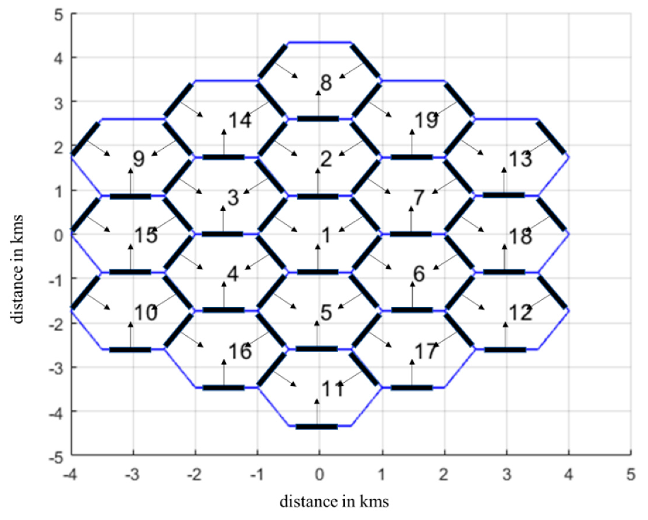
Figure 2.
Clusters and subpaths in 3GPP channel modelling.
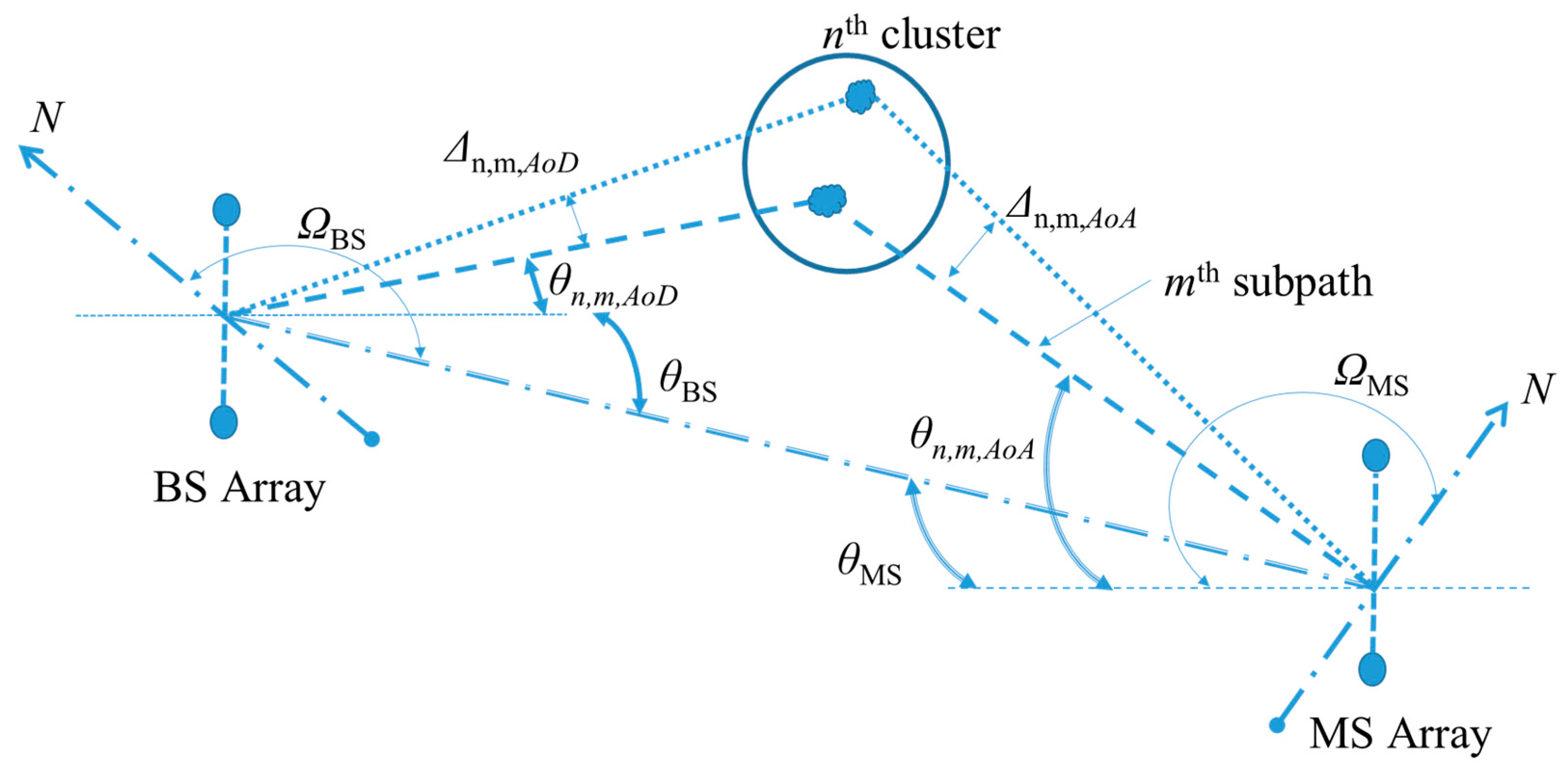
Figure 3.
The proposed antenna array scheme of 21×21 REs (left panel) along with the geometry and the radiation pattern of each RE (right panel).
Figure 3.
The proposed antenna array scheme of 21×21 REs (left panel) along with the geometry and the radiation pattern of each RE (right panel).
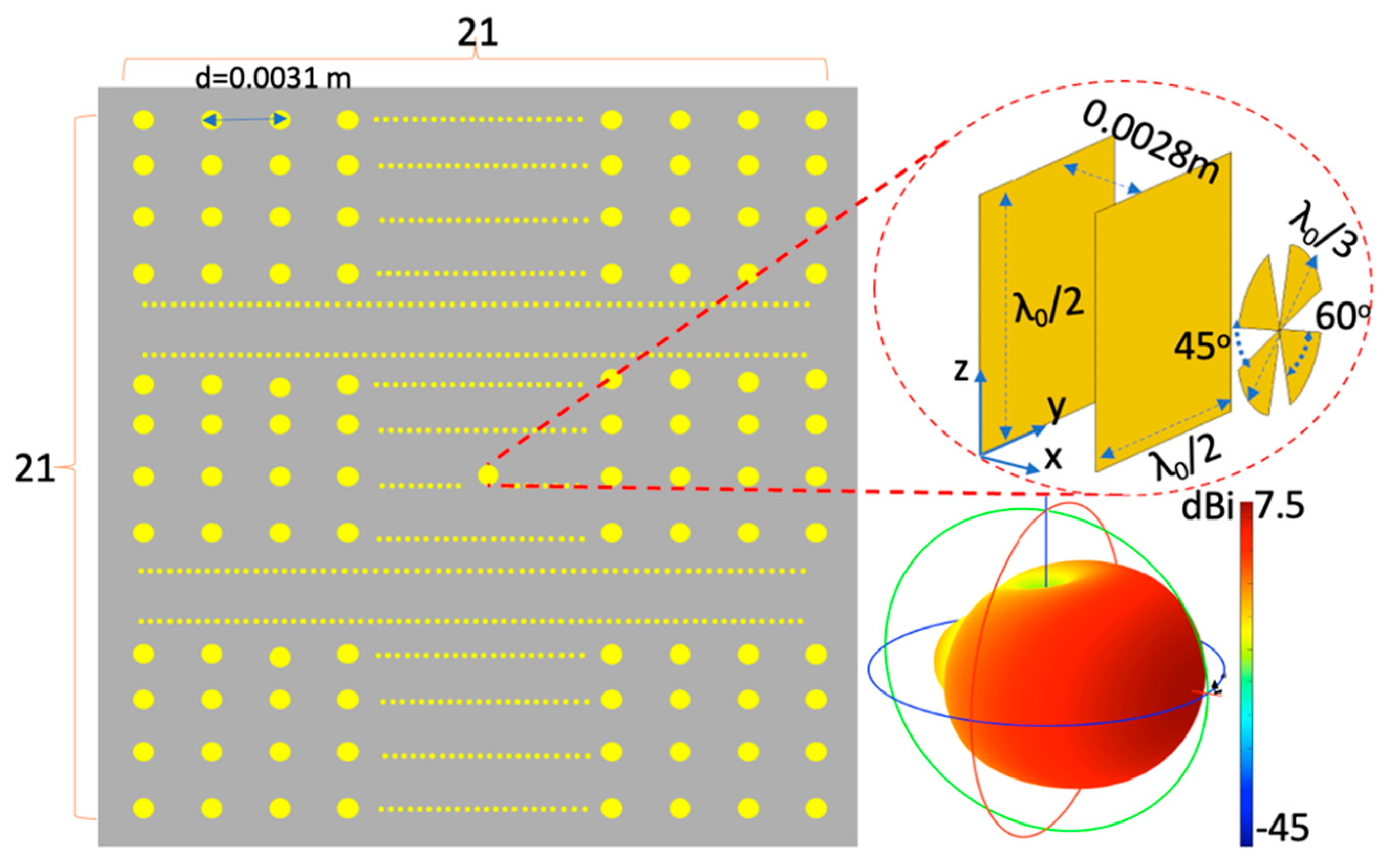
Figure 4.
Representative antenna array configurations spotted with colors (left panel) in concert with their corresponding directivity in dBi, number of REs (n) and the azimuth coverage in degrees (Φ°, upper right panel) (A representative scenario of employing different antenna array configurations for the same spatial coverage but with different services on demand is depicted at the bottom right panel).
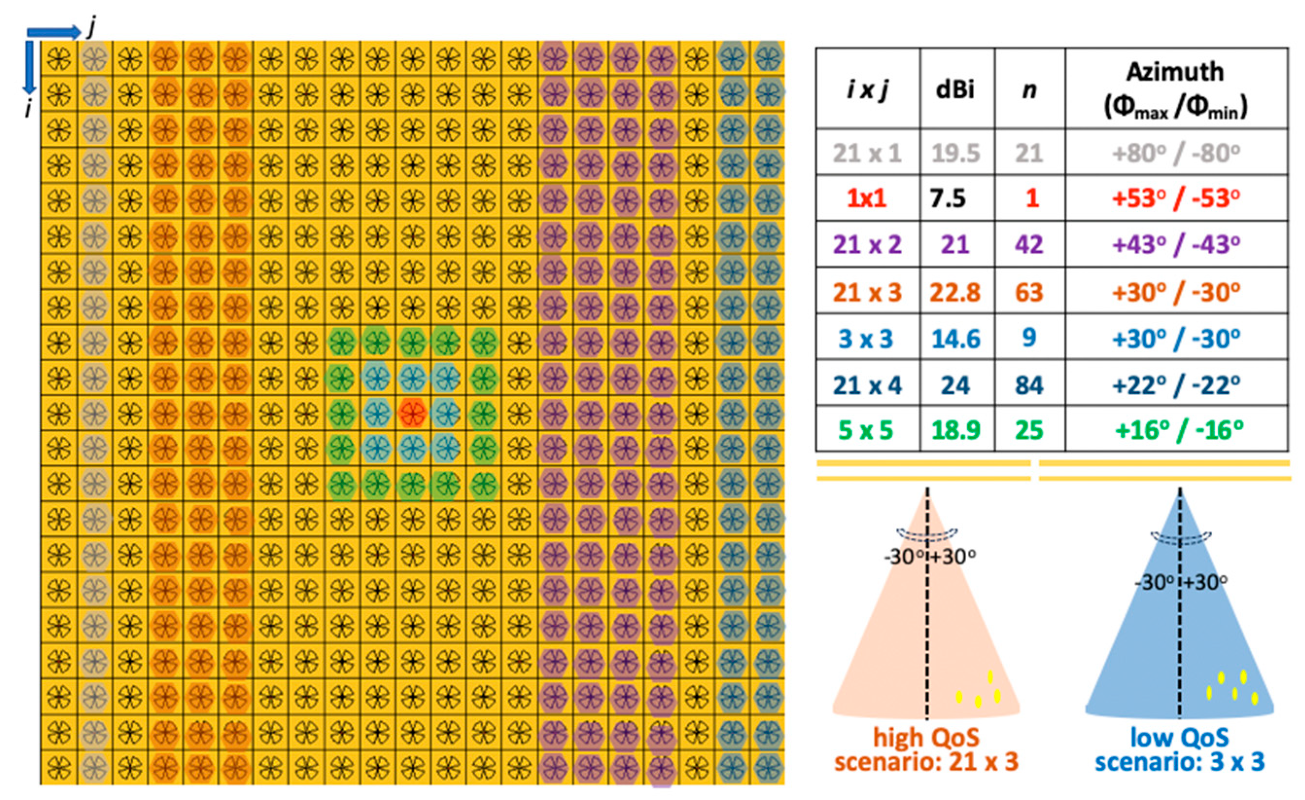
Figure 5.
Training samples aggregation.
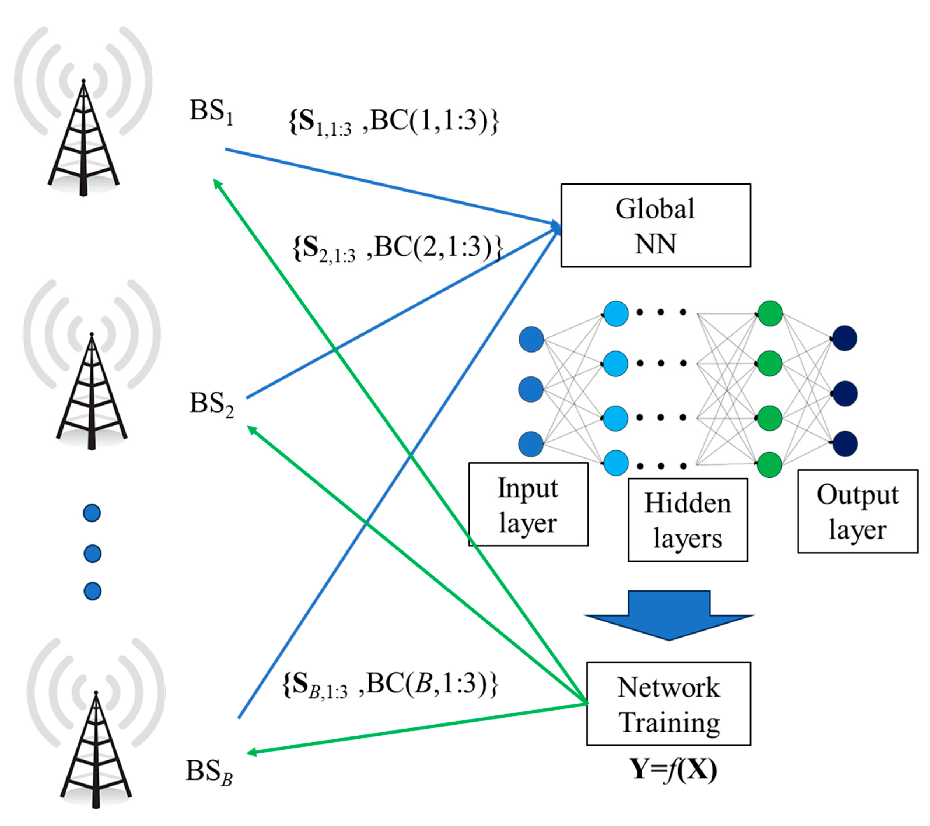
Figure 6.
Mean square error for 15 PRBs per MS and SE training.
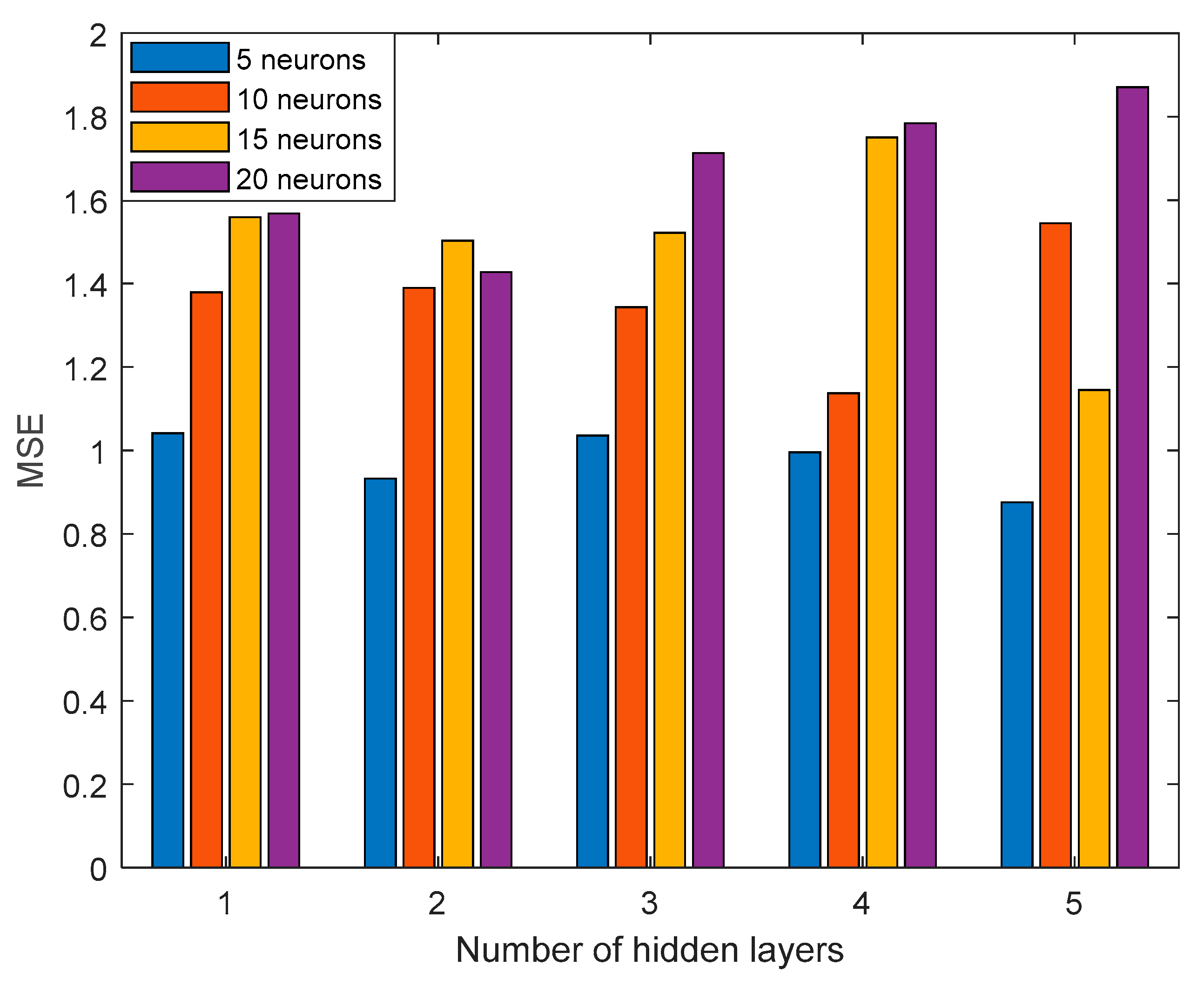
Figure 7.
Mean square error for 15 PRBs per MS and EE training.
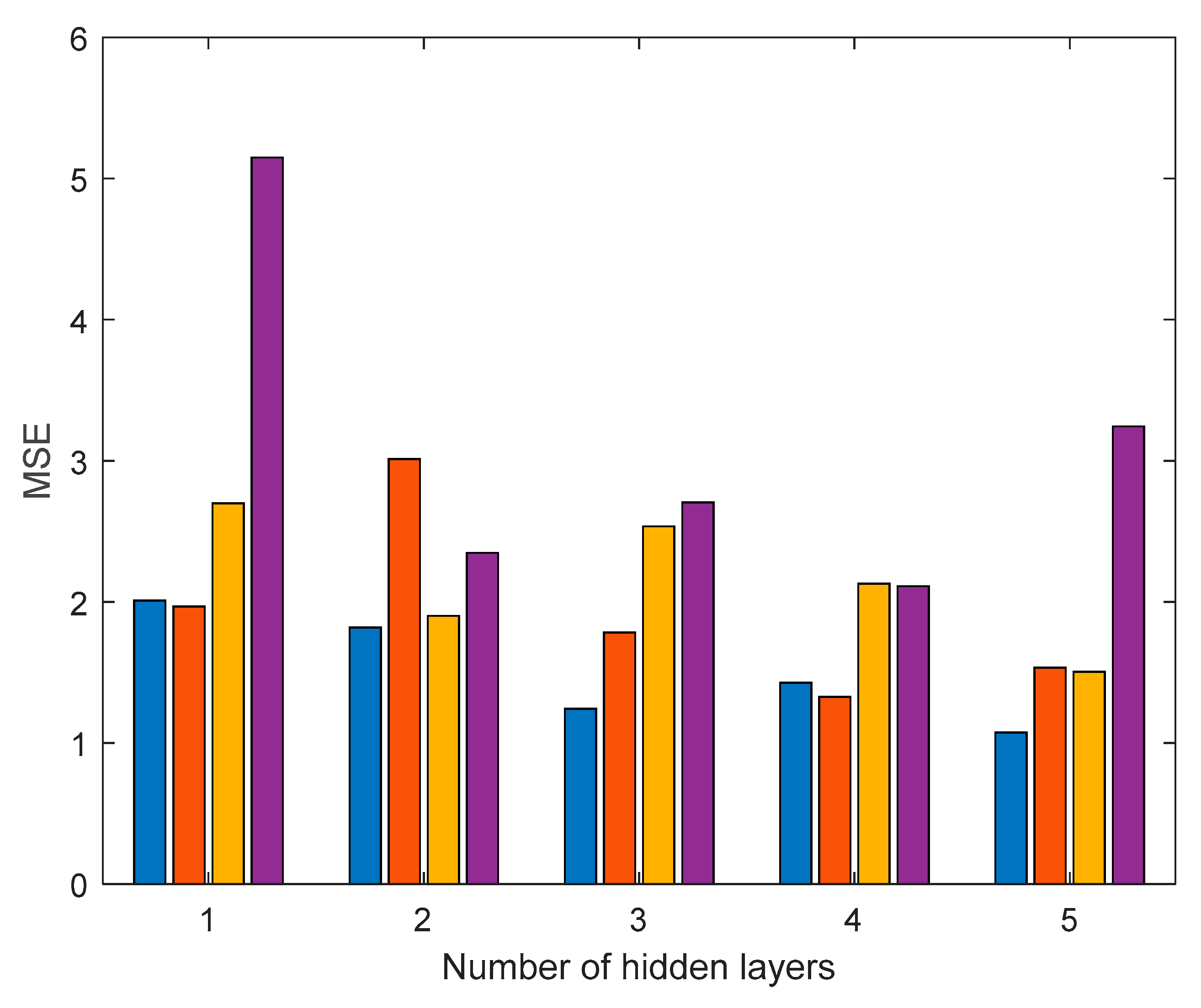
Figure 8.
Non-uniform user distribution.
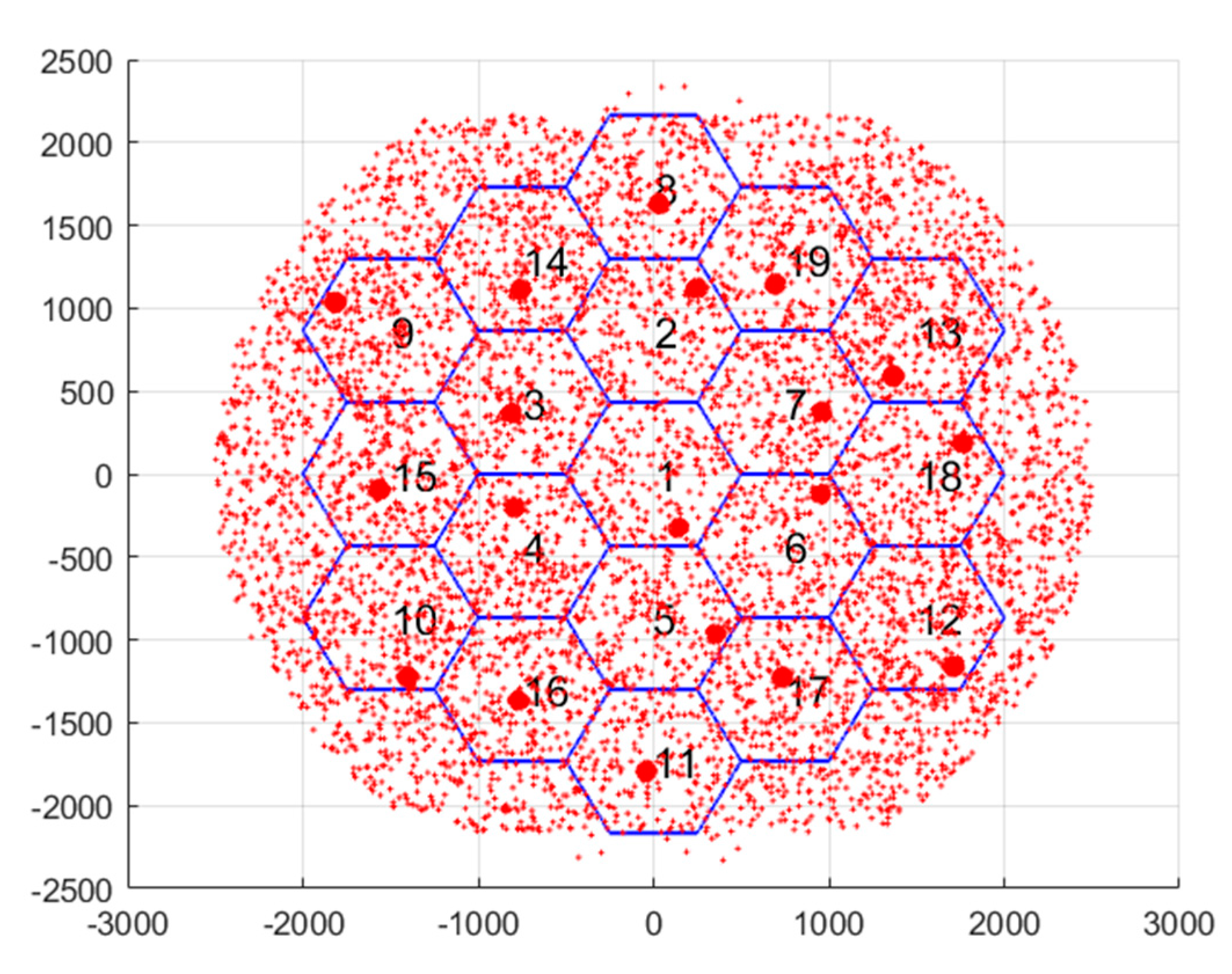
Figure 9.
Spectral Efficiency (bps/Hz).
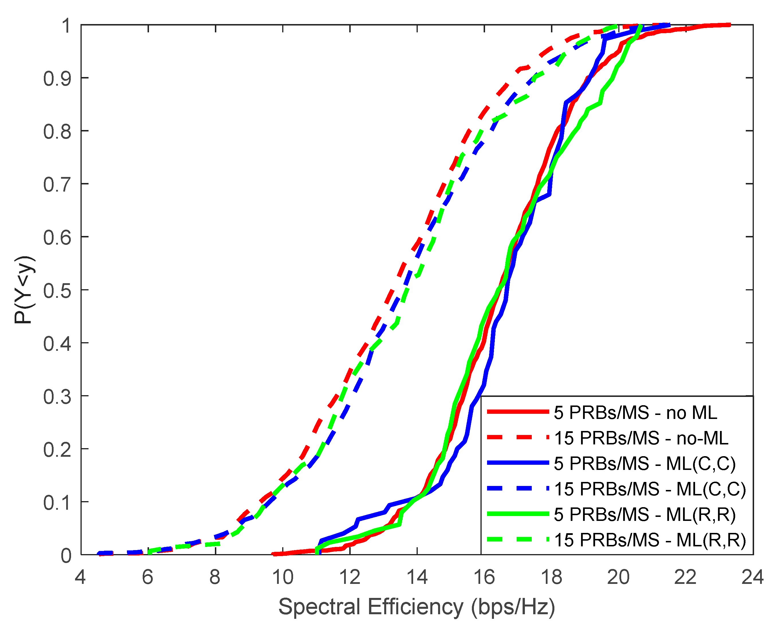
Figure 10.
Energy Efficiency (Mbps/W).
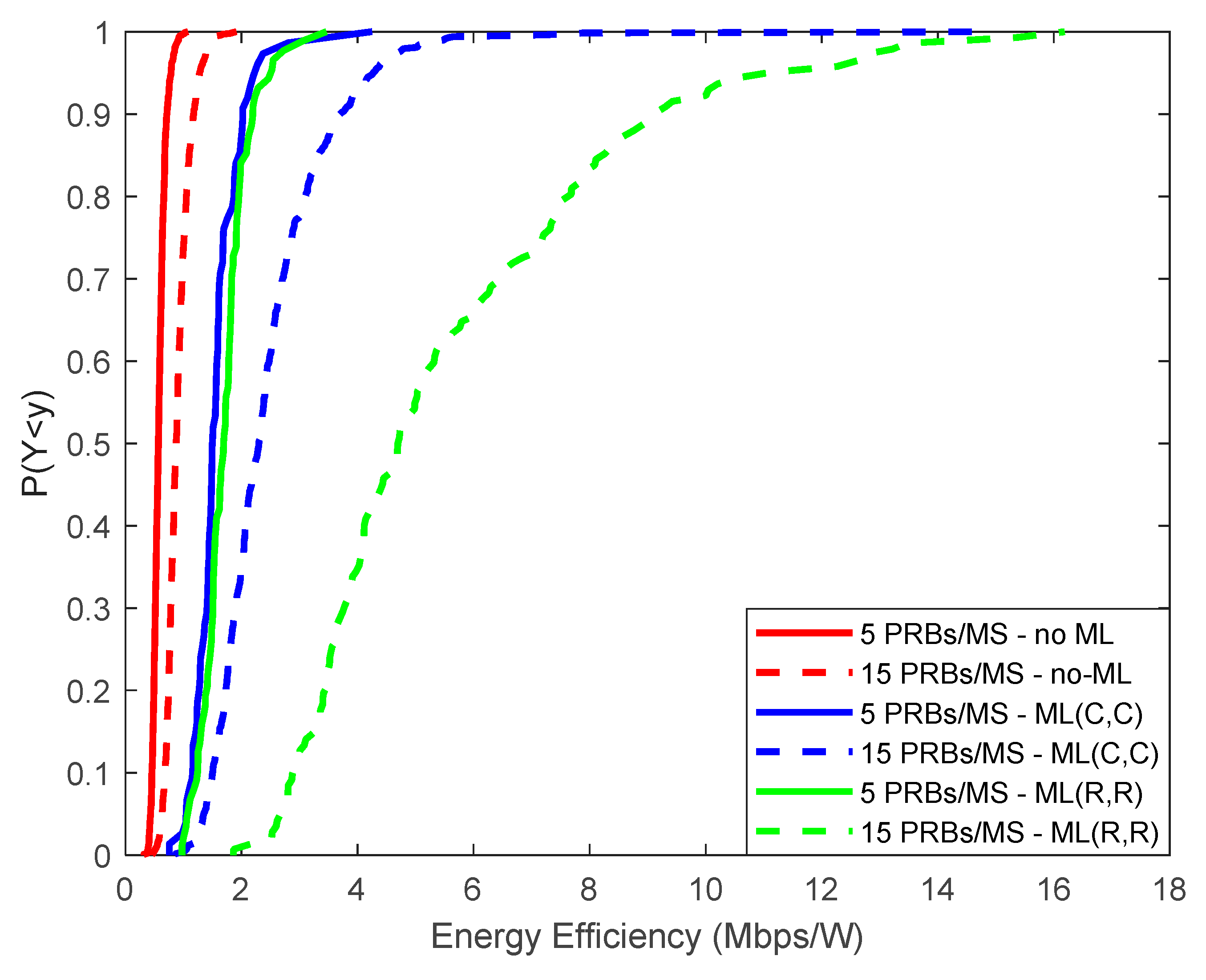
Figure 11.
Blocking probability.
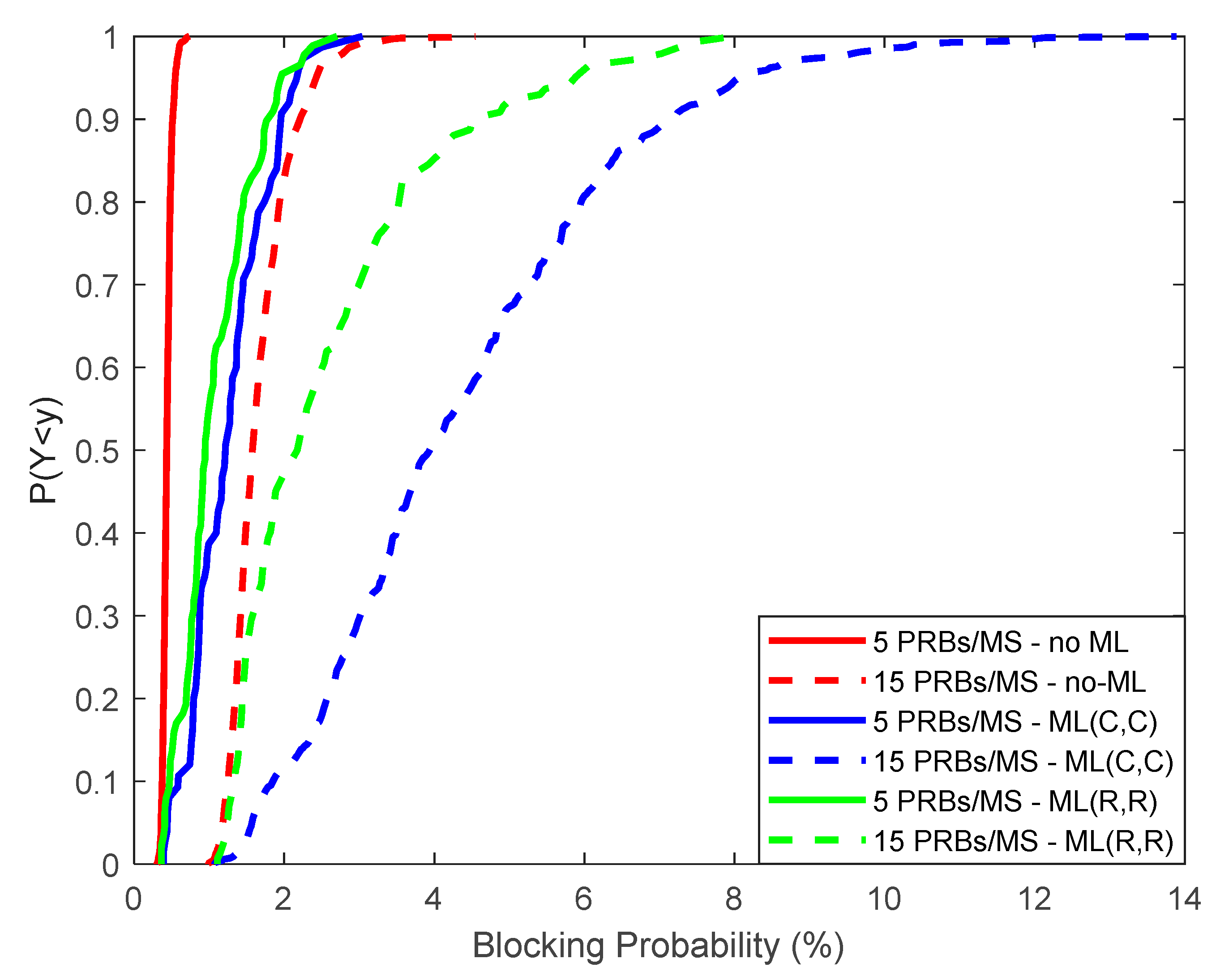
Figure 12.
Radiating elements.
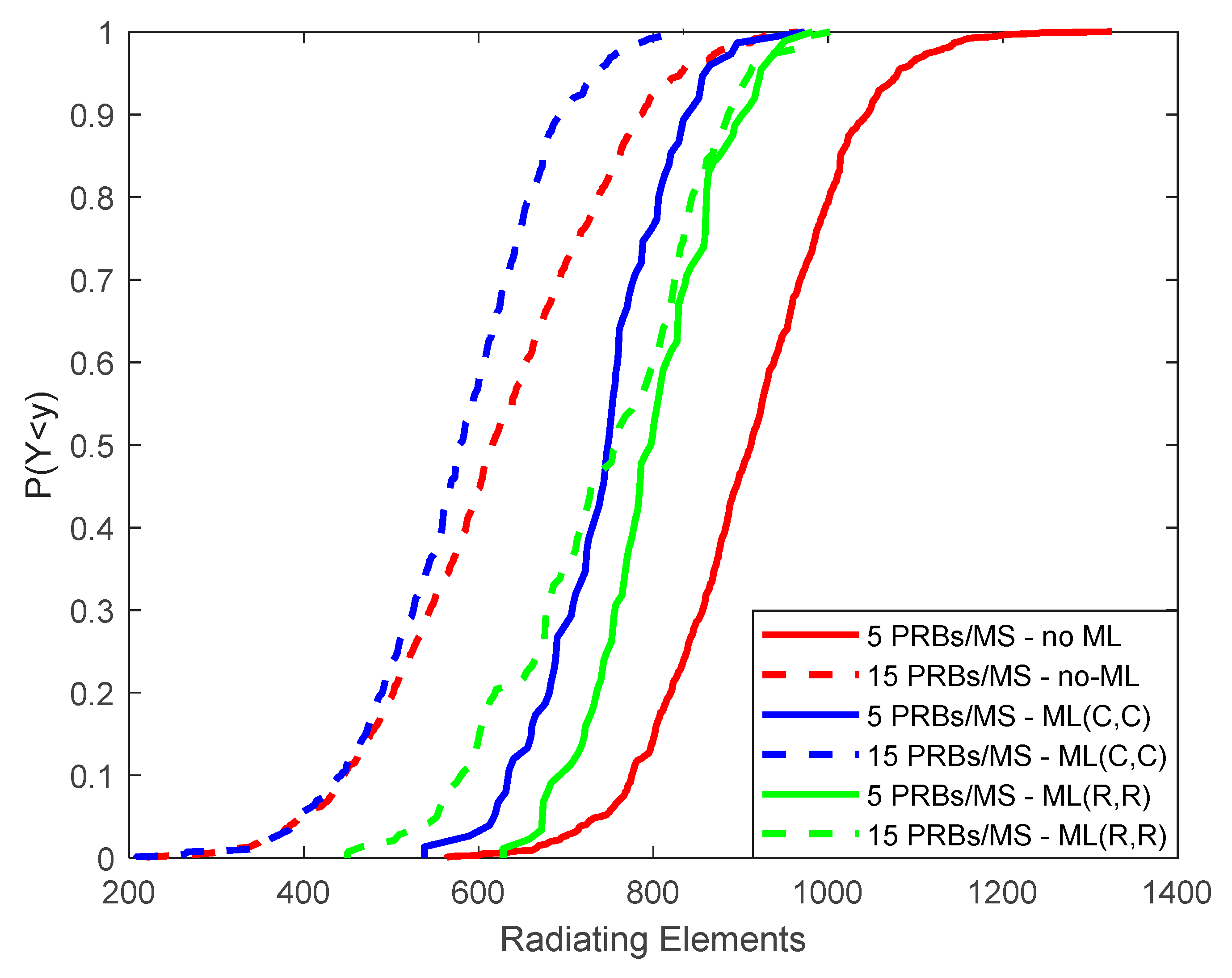

Table 1.
ML-aided adaptive beamforming.
|
Step 1: Initialization, ← {} (1≤b≤B, 1≤s≤3,), tr ← 0, XSE← O(Ns,180), XSE← O(Ns,180) Step 2: The kth MS (1≤k≤K) tries to enter the network in the sth sector of the bth BS at an angle φk requesting Rk Mbps (rf ← 0) Step 3: ← PRB_allocation(Hk,Rk) Step 4: if (~=0) then Pk ← power_allocation else rf ← 1 Step 5: if Pk>pm or set rf ← 1. Then: while (rf ==1)and(BC(b,s)<NBC) BC(b,s) ← BC(b,s) + 1 Pk ← power_allocation if Pk<pm and then rf ← 0 Step 6: if(rf==0) then tr ← tr + 1 XSE(tr,φk) ← XSE(tr,φk) + Rk/W, XEE(tr,φk) ← XEE(tr,φk) + Rk/Pk YSE(tr,1) ← BC(b,s), YEE(tr,1) ← BC(b,s) else go to Step 2 Step 7: NNSE ← train(XSE,YSE), NNEE ← train(XEE,YEE) ML mode Step 5 (updated): BC(b,s)SE ← NNSE(XSE), BC(b,s)EE ← NNEE(XEE), rf ← 0 Pk ← power_allocation if Pk>pm or then Pk ← power_allocation if Pk>pm or then rf ← 1 |
Table 2.
Simulation parameters.
| Parameter | Value |
|---|---|
| Cell radius (m) | 500 |
| Carrier frequency (GHz) | 28 |
| Total Bandwidth (MHz) | 100 |
| Pathloss model | UMa |
| Tiers of cells around the central cell/Number of cells | 2/19 |
| PRBs per MS | 5/15 |
| Modulation type per PRB | QPSK |
| Subcarrier spacing (kHz) | 60 |
| Subcarriers per PRB | 12 |
| PRBs per BS | 132 |
| Monte Carlo simulations per scenario | 104 |
| Required Eb/No (dB) for QPSK modulation [30] | 9.6 |
| Antenna elements per MS | 2 |
| Beamforming configurations (NBC) | 51 |
| Training samples per NN network | 3000 |
| Maximum power per BS/MS in W (Pm/pm) | 20/1 |
Disclaimer/Publisher’s Note: The statements, opinions and data contained in all publications are solely those of the individual author(s) and contributor(s) and not of MDPI and/or the editor(s). MDPI and/or the editor(s) disclaim responsibility for any injury to people or property resulting from any ideas, methods, instructions or products referred to in the content. |
© 2023 by the authors. Licensee MDPI, Basel, Switzerland. This article is an open access article distributed under the terms and conditions of the Creative Commons Attribution (CC BY) license (http://creativecommons.org/licenses/by/4.0/).
Copyright: This open access article is published under a Creative Commons CC BY 4.0 license, which permit the free download, distribution, and reuse, provided that the author and preprint are cited in any reuse.


