
Submitted:
18 July 2023
Posted:
19 July 2023
You are already at the latest version
Abstract
The thermal properties of a building envelope are key indicators of the energy performance of the building. Therefore, methods are needed to determine quantities like U-values or heat capacitance in a fast, reliable way and with as little impact on the use of the building as possible. In this paper a technique is proposed that relies on a simplified electrical analogical model of building envelope components which can cover their dynamic thermal behavior. The parameters of this model are optimized to produce the best fit between simulated and measured outside surface temperatures. As the temperatures can be measured remotely with an infrared camera this approach requires significantly less installation effort and intrusion in the building than other methods. At the same time, a single measurement provides data for a large range of locations on a facade or a roof. The paper describes the method and a first experimental implementation of it. The experiment indicates that this method has the potential to produce results which have an accuracy that is comparable to standardized reference methods.
Keywords:
U-value
; heat capacitance
; thermography
; model calibration
; building energy performance
1. Introduction
The high share of energy consumption in the building sector is a global concern. In most climate zones heating and cooling are responsible for the largest portion of energy consumption during the operation of a building. In the EU private households alone were responsible for 27 % of the final energy consumption in 2020. More than 60 % of this energy is used for space heating and only 27 % of this energy comes from renewables and biofuels [1]. A reduction of energy demand for heating and cooling will, therefore, help in curbing the greenhouse gas emissions. In general, there are three major factors that determine the energy performance of a building: The behaviour of the users, the efficiency of the HVAC system, and the thermophysical properties of the building envelope. A key indicator for the latter one is the heat transfer coefficient (U-value) that is given as the heat flux through an envelope element at a difference of between inside and outside air temperatures. It has been observed frequently that design values which are based on information from manufacturers of building materials or standard assumptions and U-values measured on real buildings differ significantly [2,3,4]. In addition, for many old buildings the design values are not known. So to close the energy performance gap between simulation and real energy use [5,6,7] and to provide a solid basis for decisions about possible retrofit options, fast and accurate measurement methods are required to measure real U-values of building envelopes. The heat capacitance of building envelopes is another relevant quantity for its energy performance and the user comfort as it can flatten peaks in heating and cooling demand [8].
There are standardized methods to determine the U-values of building envelope elements. These rely on averaging procedures to approximate steady-state conditions and, therefore, require relatively long measurement times of several days. The most common one is the heat flux meter (HFM) method [9] which uses air temperature sensors and heat flux meters that are attached to the building element. Therefore, they only capture the heat flow through a small area and heterogeneities are not detected.
Infrared (IR) thermography is a well known tool to qualitatively assess the insulation quality of building envelops and to find heat bridges. For many years researchers are working towards a quantitative evaluation of the thermal performance of building envelopes using thermography [10]. In 2018 a procedure standardized that is performed from the inside of a building and also attempts to approximate a steady-state measurement [11]. Such approaches can cover larger areas and inform about inhomogeneitis [12] but demand nearly constant environmental conditions, so that the measurements usually must be repeated several times [11]. Tejedor et al. propose to use statistical tests or signal modelling to reduce the necessary measurement duration [13]. However, the applicability of their analysis is limited to measurements under external conditions that lead to a steady-state heat flow through the building envelope. Attempts for quantitative external thermography with the steady-state assumption can also be found in the literature [14,15] but their outcome is, naturally, much more sensitive to changing external environment conditions.
Model calibration is an approach that does not rely on the steady-state assumption and, therefore, is expected to give higher accuracy and allow for shorter measurement times than the standardized methods [2]. In order to capture also the dynamic behaviour of the heat transport through the building, envelope models may contain also thermal capacitor or thermal mass (TM) elements. Thus, model calibration is also able to provide information about heat capacities. In literature, several approaches are found that use measured energy consumption and weather data to determine an overall heat transfer coefficient for the complete building envelope [16,17,18] which implies a strong influence of the user behavior on the results. Other approaches use heat flux meter data to identify the local U-value or thermal resistance at the respective measurement spot [2,19].
In this paper we present a model calibration approach to calculate U-values from time series of IR images that does not rely on the steady-state assumption. As we use image data, the method has the potential to give U-values for large portions of the building envelope that cover several components from a single series of measurements. At the same time, they allow for a spatial resolution of the U-values that is only limited by the resolution of the IR sensor in the camera. Therefore, it can also provide information about the homogeneity of the building envelope from a single series of measurements. In this paper we describe the general methodology of the approach and a first application to a real wall under simplified environmental conditions.
2. Method
We use a model calibration approach to determine the U-value using IR thermography. For this, teh building envelope is described by a physically informed lumped R-C model [20] as a series of resistances (R) and capacitors (C) and cover the dynamics of the heat transfer. In the first two subsections of this section the model details and the calibration procedure are described. In the third subsection we describe the experimental setup that was used to test our method on a real wall. The method is described here for a wall element. Necessary adaptations for other types of building envelop elements are discussed in Section 4.
2.1. Envelope model
The system that our model has to represent is visualized in Figure 1 for the example of a wall element. In the R-C model the wall is modelled as a series of thermal resistors and TM. The internal and external boundary conditions are calculated from measured time series of environmental parameters.
We build the model using the open source modelling language Modelica. The models for the individual resistor and capacitor elements of the wall are taken from the Modelica Standard Library [21]. The visualization by the OpenModelica Connection Editor [22] of a model with two TM and three resistors (2TM model) is shown in Figure 2. It represents a set of differential equations that approximate a one-dimensional heat flow through the wall.
A thermal resistor element stands for
where q is the heat flux, is the thermal resistance of the element, A its area, and are the temperatures on the right and left side of the element, respectively. The capacitor or TM elements stand for
where C is the heat capacity and is the derivative of T with respect to time. The connections with red lines mean that the temperatures at the connected points are set equal and that the heat flux into one element equals the heat flux out of the other element. If one element is connected to more than a single other element it means that the heat fluxes of those other elements are summed up.
In priciple, an arbitrary number of alternating resistor and TM elements can be used. Smaller numbers of elements lead to a smaller parameter space which reduces the time of the calibration process. Larger numbers are more realistic representations of the real wall and, especially, reproduce fast surface effects better that can appear, e.g., due to changing direct solar irradiation. Models with two TM and three resistors have turned out to be a good trade-off in a series of experiments that we ran and are frequently used in the literature [2,23,24]. If the wall is known to be approximately symmetric the number of parameters can be further reduced by setting equal the resistances of the outer and inner resistor elements and the thermal capacities of the two TM.
The boundary conditions are determined by the internal and external environmental conditions that are illustrated in Figure 1. There are three processes that are considered here and add up as contributions to the boundary conditions. One is convective heat exchange between the wall and the surrounding air. Another one is the exchange of thermal long-wave (LW) radiation between the wall and surrounding surfaces. And the third one is the absorption of solar short-wave (SW) radiation. In our case we only consider short-wave radiation coming from the sun. The convective term is given by
where h is the convective heat transfer coefficient, is the surface temperature of the wall and is the air temperature. The long-wave radiation term is given by
where is the emittance of the wall surface in the thermal infrared range, is the Stefan–Boltzmann constant, and is a weighted average over the radiation temperatures of the surrounding objects. The short-wave radiation term is given by
where is the absorptance of the wall surface in the short-wave range and is the global tilted solar irradiance that hits the wall surface and depends on the position of the sun and the orientation of the wall. In order to solve the differential equations, the minimum required knowledge to provide these boundary conditions are the inside and outside air temperature and the global tilted solar irradiance which can be measured directly or calculated from other solar irradiance measurements.
The whole system of ordinary differential equations with boundary conditions is implemented in Modelica. Given the values of all parameters and the external conditions it can be solved to obtain heat fluxes and temperatures for each element at every moment in time. We choose literature values for for the emittance, the short wave absorptance, and the indoor convective heat transfer coefficient . On the outside the choice of h depends on the wind conditions. In a protected spot with no or almost no wind the convective heat transfer coefficient can be calculated using the Nusselt number that depends on and [25] as
where k is the thermal conductivity of the wall and L is its height. If the wind speed implies forced convection an appropriate model must be chosen according to the site-specific conditions. For many situations the model by Liu and Harris [26] provides a good trade-off between accuracy and simplicity. The U-value is obtained from these quantities as
2.2. Model calibration
While the external and internal environment conditions can be determined directly by measurements, the thermal resistances and capacities of the model elements that represent the bulk wall cannot be accessed by a direct measurement. However, these are particularly interesting because they give a major contribution to the U-value of the wall and are responsible for its thermal storage properties. These are determined by the model calibration process. We record a time series of surface temperatures using an IR camera together with the environmental conditions that determine the boundary conditions. Then we optimize the unknown resistances and capacities of the model, so that the surface temperature predicted by the model, given the recorded environmental conditions, and the measured time series of surface temperatures fit as well as possible. We have implemented the optimization in a Python script that interfaces with the Modelica model through OMPython [22]. We use the Levenberg-Marquardt method that is implemented in the LMFIT package [27] to minimize the objective function
where N is the number of time steps for that measurements were taken, and are the measured and predicted temperatures at time step i, respectively, is the estimated uncertainty of the measured temperature at time step i, is a vector that contains the resistance values of the model elements, and is a vector that contains the capacity values of the model elements.
To assess the quality of the fit we also calculate the reduced chi-square after the optimization as
where is the number of optimized parameters. The total thermal resistance for an element of a location is the sum over the resistances of the resistor elements in the model.
2.3. Experimental setup
The experimental test of the proposed method is performed on a small test building which is shown in Figure 3a. The wall that we used for the experiment is made of pumiced stone with light weight concrete and has an area of . It is a plastered single-layer wall and it has a U-value of according to the manufacturer. The building was heated with a portable fan electrical heater inside. To reduce the complexity of the experiment, a tent was constructed over the test building (see Figure 3b), so that short-wave solar irradiance and wind speed can be neglected on the outside.
Figure 4 shows the setup of the measurement spot. For reference measurements we use two heat flux sensors which are installed directly on the bricks and covered with plaster. Another heat flux sensor is attached to the outer surface of the wall and one on the opposite side of the wall inside of the building. The surface temperatures were also measured with two NTC contact sensors. But their measurements are not used in the following parts of this paper. An additional temperature sensor is mounted on the wall but not attached to the surface, so that it measures the air temperature near the wall surface. Inside the building, another air temperature sensor is installed. Two patches of crumbled aluminium foil are attached to the wall. They serve as diffuse reflectors for long-wave radiation and are used to determine the long-wave radiation coming from surrounding surfaces which is required to calculate the correct wall surface temperature and in Equation 4 [12,28].
The IR camera was placed approximately five meters away from the wall on a tripod. Its field of view covers the complete scene that is shown in Figure 4. We used a freshly calibrated microbolometer camera with an accuracy of and a wave length range from to . As the IR camera that was used for the experiment did not correct properly for the varying radiation from its housing and the readings changed with the outside air temperature, this correction had to be done in the post processing. In Figure 4 two self-made black bodies can be seen in the bottom. These had different temperatures and served as references for the correction process. We assumed a linear dependence between the housing temperature and the deviation between the measured and real surface temperatures in the relevant temperature range. This allows for estimating a simple linear correction function.
3. Experimental Results
An examplary image of the IR measurement is shown in Figure 5. In the experiment a series of images was taken for five days with a frequency of one image per minute. We chose a region of approximately in the scene (see Figure 5) on the wall and used the manufacturer’s software to extract the average temperature for this region in every image. Various values are reported in the literature for the emittance of plaster but they are from a rather narrow range [29,30,31]. For our calculation, we choose and for the indoor convective heat transfer coefficient [32].
Figure 6 shows the complete time series of IR temperature measurements together with the outcome of a simulation with the optimized set of resistance and capacitance values. For validation purposes, simultaneous measurements of the NTC and heat flux sensors were taken. Using these values with the standard heat flux meter method [9], a reference U-value can be calculated from the air temperature and heat flux data. We find which corresponds to a thermal resistance of . The model calibration is used to determine the resistance values of the resistor elements in the model which sum up to the total thermal resistance of the wall. The calibration is performed for the complete time series of five days and several intervals within this series. The results can be found in Table 1.
The U-value determined by the model calibration approach is between and higher than the reference value () and between and higher than the U-value given by the manufactuerer (). A further observation is that small correlate with small deviations from the reference U-value. The same observation is made if the manufacturer’s value is used as reference. We also observe that the U-values that come from the model calibration appear to lie systematically higher than the reference value. However, as the reference comes from a single measurement which also carries errors from measurement uncertainties, an uncertainty analysis is performed in Section 3.1 and Section 3.2 to find out whether the results of the new method are compatible with the reference.
The HFM method does not give a reference value for the heat capacity. Table 1 shows that the relative variations of the heat capacity are stronger among the different time periods than for the thermal resistance. We cannot identify a clear correlation between the values of C and , either. This indicates that the fit quality is not very sensitive to the value of the heat capacity. We confirmed this by some experiments where we kept the heat capacities constant during the fit and found a weak dependence of the resulting thermal resistance on the chosen capacities.
3.1. Uncertainty analysis of the HFM method
ISO 9869-1:2015 [9] explains how much uncertainty should be considered for each parameter in the HFM method. It depends on the following factors,
- Approx. error due to the accuracy of the calibration of the HFM and temperature sensors if the sensors are well calibrated.
- Approx. variation due to slight difference in thermal contact between HF sensor and the wall surface.
- to uncertainty due to operational error of the HFM.
- Approx. error caused by the variations over time of the temperatures and heat flow.
- Approx. error in U-value measurement due to temperature variations within the space and difference between air and radiant temperatures.
These above uncertainty factors are added to produce the total uncertainty. The norm ISO 9869-1:2015 says that if the suggested measurement conditions are fulfilled, the total uncertainty shall be expected to be between the quadrature sum and arithmetic sum [9]. As a result, it stays between to . As the U-value that is measured with the HFM method is the confidence interval ranges in the worst case from to and clearly covers the U-values obtained by the calibration method.
3.2. Uncertainty analysis of the model calibration approach
To determine the error of the thermal resistance obtained by the calibration method, we have to estimate the error in the input quantities. For the quantities that we measure directly or indirectly we rely on information about measurement errors from the manufacturers. The error in the emittance is estimated from the range of different values for plaster in the literature [29,30,31]. The error in the internal convective heat transfer coefficient is based on an ISO standard [32]. We assume a rather large error here to account for the fact that the indoor conditions are not observed in our scenario. The errors are shown in Table 2. We perform a latin hypercube sampling of the values assuming a normal distribution with the given error as standard deviation. Each sample is a different set of values for the input quantities. For each sample the calibration is performed using the complete time series of five days. We set a threshold of to filter out samples that clearly show a bad fit and determine the mean and standard deviation of the remaining ones. We vary the number of samples from 10 to 1000 to check for what sample size the mean and standard deviation of the thermal resistance converges. Figure 7 shows that for >500 samples we can consider the process as converged. So we find that the converged mean total thermal resistance is and the corresponding standard deviation is which corresponds to an error of . This means that the reference value determined by the HFM method lies within the interval of the result that we obtained with our calibration method.
4. Discussion
This paper presents a model calibration approach to determine the thermal resistance, capacitance and, consequently, the U-value of building envelope elements from remote surface temperature measurements with an IR camera. The envelope element is modelled with a lumped R-C-type model and is calibrated by minimizing an objective function that compares the measured and simulated external surface temperature of the element. We reported an experiment using infrared cameras to test the method on a real wall and compare the outcome to a standardized reference HFM measurement. The measurement data gives very consistent results of the thermal resistance for various time intervals ranging from a single day to five days, while standard methods usually require measurement periods of up to seven days [9]. The large variation in the heat capacity among the different intervals indicates that the approach is less well suited to accurately determine this quantity for a building wall. We have performed an uncertainty analysis of our method for the same dataset and a standard reference measurement of the U-value that uses HFM. It turns out that the confidence intervals overlap which indicates that the new method achieves a satisfactory accuracy. The reduced chi-square of the model fit appears to be a good indicator for the success of the calibration process and the accuracy of the resulting U-value. High may indicate large measurement errors or inadequate assumptions for input quantities.
The experiment was performed under simplified conditions: Short-wave solar radiation and wind speed could be assumed to be zero because the test building and the surrounding area were covered with a tent. While the solar irradiation onto the wall can be easily measured and modelled it may lead to rapid changes in the temperature of the wall close to the outer surface. Such effects may require wall models with more than 2 thermal masses and three resistors. The wind, on the other hand, is less likely to cause such surface-effects. However, the wind speed varies significantly in front of large walls, so that a measurement in one or few locations may not be representative for the complete surface. The model that is chosen to connect wind speed and the surface heat transfer coefficient will also change the calibration outcome. So further tests under full environmental conditions are necessary to determine the conditions under which our method reliably gives accurate results for the U-value.
In the experiment that we reported we used the temperature average of a single relatively small area to perform the model calibration. The same procedure can be run for additional areas on the wall to obtain the thermal resistance and U-value with a spatial resolution on the wall. The size and the number of the averaging areas must be chosen according to the respective measurement task. Small areas will likely introduce some noise in the resistances because noise coming from the camera measurements is not averaged out. If the area is large it increases the chance that inhomogeneities are missed.
It is desirable to use the method also for other components of building envelopes than in our example. The necessary adaptations mainly depend on the reflective properties of the surface material. Most usual plasters, bare bricks, wooden surfaces, dull tiles, or many plastic materials will only require a change of the emittance for long-wave radiation and the absorptance for short-wave radiation in the model. Metallic surfaces often have high reflectance in the long-wave range. The issue that diffuse reflection may dominate over specular reflection does not require a change in the methodology or setup. However, a strong contribution of reflected radiation to the measurement by the IR camera may impact the accuracy. Materials that reflect the long-wave thermal radiation specularly, e.g. glass, must be treated in a different way to subtract the signal of any hot object being reflected on the measurement surface. Different approaches will be tested in future.
To conclude, the presented method offers an efficient way to determine the U-values of a building wall with very little effort of sensor installation and potentially shorter measurement time than conventional methods in the standards. An experiment on a real wall with simplified environmental conditions indicates that its accuracy is at least comparable to the reference heat flux meter method. Further tests and validation steps must be undertaken to ensure the reliability of the method under full environmental conditions and for surface materials with reflective properties that differ significantly from those of the plaster in our experiment.
Author Contributions
Conceptualization, Jacob Estevam Schmiedt and Marc Röger; software, Dhruv Patel; validation, Dhruv Patel; writing—original draft preparation, Jacob Estevam Schmiedt; writing—review and editing, Dhruv Patel and Marc Röger; supervision, Bernhard Hoffschmidt; project administration, Jacob Estevam Schmiedt and Marc Röger; funding acquisition, Jacob Estevam Schmiedt. All authors have read and agreed to the published version of the manuscript.
Funding
This research was funded by the German Federal Ministry for Economic Affairs and Climate Action.
Institutional Review Board Statement
Not applicable.
Informed Consent Statement
Not applicable.
Data Availability Statement
The data that is required to understand the method and experiments presented in this paper are is given in the text. Additional data, e.g., raw measurement data can be provided upon request by the authors.
Acknowledgments
The authors would like to thank Johannes Pernpeintner for his support with the experiment and helpful discussions of the methodology.
Conflicts of Interest
The authors declare no conflict of interest. The funders had no role in the design of the study; in the collection, analyses, or interpretation of data; in the writing of the manuscript; or in the decision to publish the results.
Abbreviations
The following abbreviations are used in this manuscript:
| C | capacitor |
| EU | European Union |
| HFM | Heat flux meter |
| LW | long wave |
| HVAC | Heating, ventilation, air-conditioning, and cooling |
| IR | Infrared |
| R | resistance |
| SW | short wave |
| TM | Thermal mass |
References
- European Commission. Statistical Office of the European Union. Energy consumption in households 2022.
- Gori, V.; Marincioni, V.; Biddulph, P.; Elwell, C.A. Inferring the thermal resistance and effective thermal mass distribution of a wall from in situ measurements to characterise heat transfer at both the interior and exterior surfaces. Energy and Buildings 2017, 135, 398–409. [Google Scholar] [CrossRef]
- Teni, M.; Krstić, H.; Kosiński, P. Review and comparison of current experimental approaches for in-situ measurements of building walls thermal transmittance. Energy and Buildings 2019, 203, 109417. [Google Scholar] [CrossRef]
- Li, F.G.N.; Smith, A.; Biddulph, P.; Hamilton, I.G.; Lowe, R.; Mavrogianni, A.; Oikonomou, E.; Raslan, R.; Stamp, S.; Stone, A.; Summerfield, A.; Veitch, D.; Gori, V.; Oreszczyn, T. Solid-wall U-values: heat flux measurements compared with standard assumptions. Building Research & Information 2014, 43, 238–252. [Google Scholar] [CrossRef]
- de Wilde, P. The gap between predicted and measured energy performance of buildings: A framework for investigation. Automation in Construction 2014, 41, 40–49. [Google Scholar] [CrossRef]
- van Dronkelaar, C.; Dowson, M.; Spataru, C.; Mumovic, D. A Review of the Regulatory Energy Performance Gap and Its Underlying Causes in Non-domestic Buildings. Frontiers in Mechanical Engineering 2016, 1. [Google Scholar] [CrossRef]
- Cozza, S.; Chambers, J.; Brambilla, A.; Patel, M.K. In search of optimal consumption: A review of causes and solutions to the Energy Performance Gap in residential buildings. Energy and Buildings 2021, 249, 111253. [Google Scholar] [CrossRef]
- Olsthoorn, D.; Haghighat, F.; Moreau, A.; Lacroix, G. Abilities and limitations of thermal mass activation for thermal comfort, peak shifting and shaving: A review. Building and Environment 2017, 118, 113–127. [Google Scholar] [CrossRef]
- ISO-9869-1. Thermal Insulation-Building Elements-In-situ Measurement of Thermal Resistance and Thermal Transmittance-Part 1: Heat Flow Meter Method. ISO 2015.
- Martin, M.; Chong, A.; Biljecki, F.; Miller, C. Infrared thermography in the built environment: A multi-scale review. Renewable and Sustainable Energy Reviews 2022, 165, 112540. [Google Scholar] [CrossRef]
- ISO-9869-2. Thermal Insulation-Building Elements-In-situ Measurement of Thermal Resistance and Thermal Transmittance - Part 2: Infrared method for frame structure dwelling. ISO 2018.
- Marshall, A.; Francou, J.; Fitton, R.; Swan, W.; Owen, J.; Benjaber, M. Variations in the U-Value Measurement of a Whole Dwelling Using Infrared Thermography under Controlled Conditions. Buildings 2018, 8. [Google Scholar] [CrossRef]
- Tejedor, B.; Casals, M.; Macarulla, M.; Giretti, A. U-value time series analyses: Evaluating the feasibility of in-situ short-lasting IRT tests for heavy multi-leaf walls. Building and Environment 2019, 159, 106123. [Google Scholar] [CrossRef]
- Patel, D.; Schmiedt, J.E.; Röger, M.; Hoffschmidt, B. Approach for external measurements of the heat transfer coefficient (U-value) of building envelope components using UAV based infrared thermography. 14th Quantitative Infrared Thermography Conference QIRT, 2018.
- Mahmoodzadeh, M.; Gretka, V.; Hay, K.; Steele, C.; Mukhopadhyaya, P. Determining overall heat transfer coefficient (U-Value) of wood-framed wall assemblies in Canada using external infrared thermography. Building and Environment 2021, 199, 107897. [Google Scholar] [CrossRef]
- Rouchier, S.; Rabouille, M.; Oberlé, P. Calibration of simplified building energy models for parameter estimation and forecasting: Stochastic versus deterministic modelling. Building and Environment 2018, 134, 181–190. [Google Scholar] [CrossRef]
- Rouchier, S.; Jiménez, M.J.; Castaño, S. Sequential Monte Carlo for on-line parameter estimation of a lumped building energy model. Energy and Buildings 2019, 187, 86–94. [Google Scholar] [CrossRef]
- Shamsi, M.H.; Ali, U.; Mangina, E.; O’Donnell, J. A framework for uncertainty quantification in building heat demand simulations using reduced-order grey-box energy models. Applied Energy 2020, 275, 115141. [Google Scholar] [CrossRef]
- Prada, A.; Gasparella, A.; Baggio, P. A Robust Approach For The Calibration Of the Material Properties in an Existing Wall. Proceedings of the 16th IBPSA Conference, 2019.
- Paschkis, V.; Baker, H.J.T.A. A method for determining unsteady state heat transfer by means of an electrical analogy. Transaction of the American Society of MechanicalEngineers 1942, 64, 105–112. [Google Scholar] [CrossRef]
- Fritzson, P., The Modelica Standard Library. In Introduction to Modeling and Simulation of Technical and Physical Systems with Modelica; John Wiley & Sons, Ltd, 2011; chapter 5, pp. 157–168, [https://onlinelibrary.wiley.com/doi/pdf/10.1002/9781118094259.ch5]. [CrossRef]
- OpenModelica User’s Guide 2022.
- Dewson, T.; Day, B.; Irving, A. Least squares parameter estimation of a reduced order thermal model of an experimental building. Building and Environment 1993, 28, 127–137, Special Issue Thermal Experiments in Simplified Buildings. [Google Scholar] [CrossRef]
- Berthou, T.; Stabat, P.; Salvazet, R.; Marchio, D. Development and validation of a gray box model to predict thermal behavior of occupied office buildings. Energy and Buildings 2014, 74, 91–100. [Google Scholar] [CrossRef]
- Ghajar, A.J.; others. Heat and mass transfer; McGraw-Hill,, 2015.
- Liu, Y.; Harris, D. Full-scale measurements of convective coefficient on external surface of a low-rise building in sheltered conditions. Building and Environment 2007, 42, 2718–2736. [Google Scholar] [CrossRef]
- Newville, M.; Stensitzki, T.; Allen, D.B.; Ingargiola, A. LMFIT: Non-Linear Least-Square Minimization and Curve-Fitting for Python 2014. [CrossRef]
- ISO-18434-1. Condition Monitoring and Diagnostics of Machines. Thermography Part 1: General Procedures. ISO 2008.
- Kolokotsa, D.; Maravelaki-Kalaitzaki, P.; Papantoniou, S.; Vangeloglou, E.; Saliari, M.; Karlessi, T.; Santamouris, M. Development and analysis of mineral based coatings for buildings and urban structures. Solar Energy 2012, 86, 1648–1659. [Google Scholar] [CrossRef]
- Engineering ToolBox, Emissivity Coefficients common Products [online] 2003.
- Marshall, S.J. We Need To Know More About Infrared Emissivity. SPIE Proceedings, Thermal Infrared Sensing Applied to Energy Conservation in Building Envelopes; Grot, R.A.; Wood, J.T., Eds. SPIE, 1982. [CrossRef]
- ISO-6946. Building components and building elements–thermal resistance and thermal transmittance–calculation method. ISO 2017.
Figure 1.
Sketch of processes that determine the heat flow through a wall element.
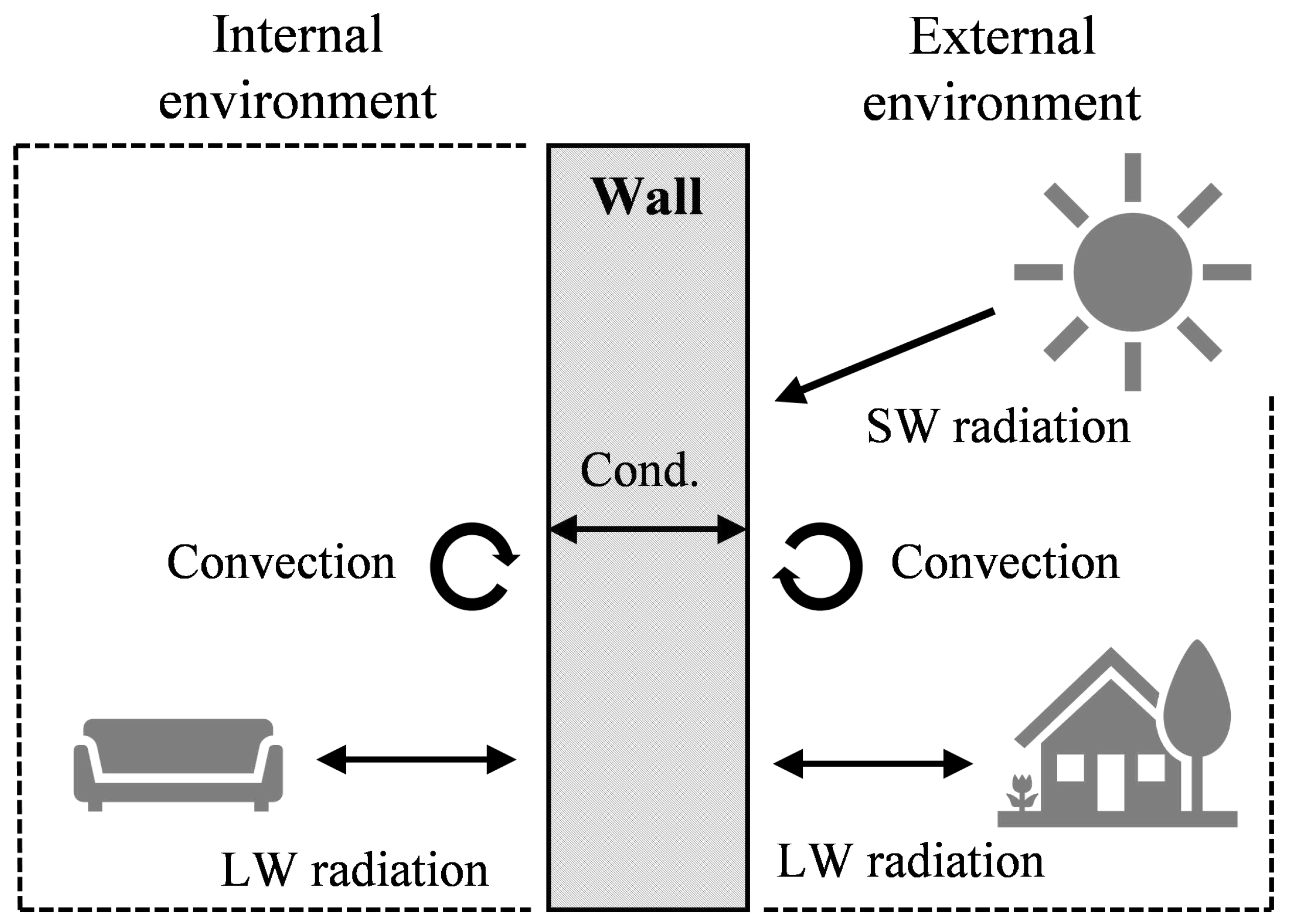
Figure 2.
2TM wall model without the boundary conditions.
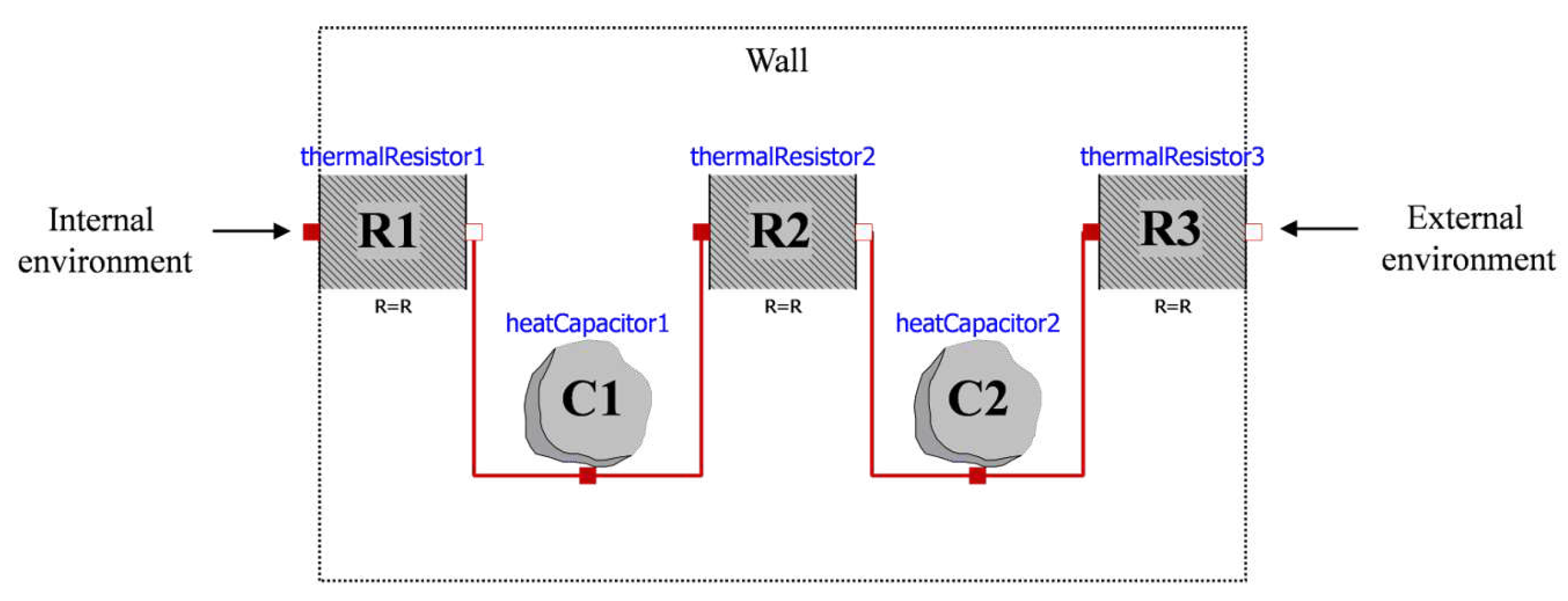
Figure 3.
The test building without (a) and with covering tent (b).
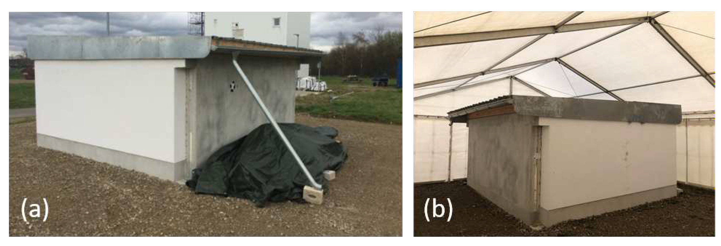
Figure 4.
The setup of sensors for validation purposes on the measured wall and two blackbodies in front of it. The blackbodies are used to have a better control of the IR camera uncertainty. The patches of aluminium foil serve as a diffuse reflectors for thermal radiation from surrounding objects.
Figure 4.
The setup of sensors for validation purposes on the measured wall and two blackbodies in front of it. The blackbodies are used to have a better control of the IR camera uncertainty. The patches of aluminium foil serve as a diffuse reflectors for thermal radiation from surrounding objects.
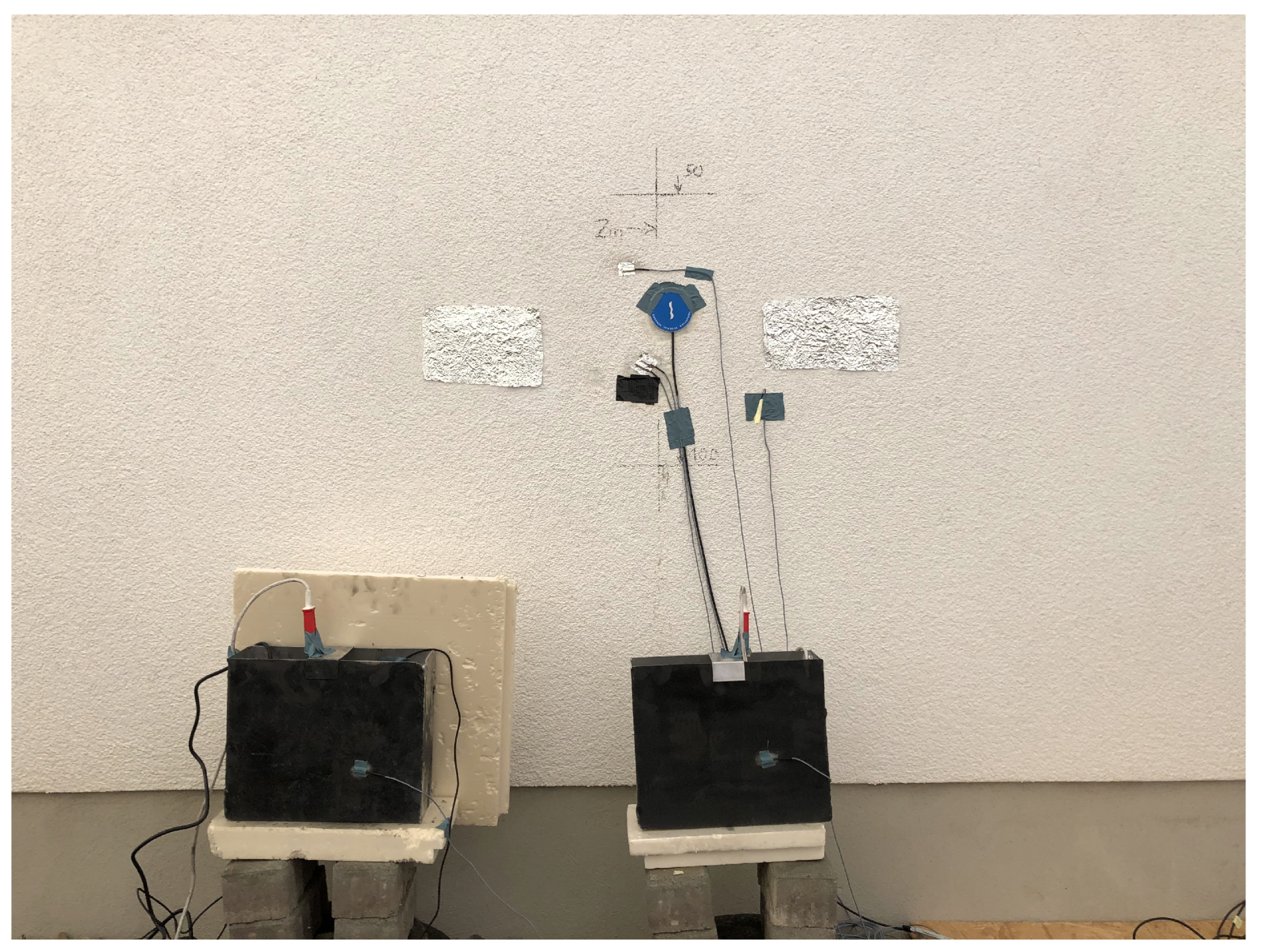
Figure 5.
An exemplary image from the IR time series. For the model calibration the temperature of a small area that is marked with a yellow square and denoted A1 was used.
Figure 5.
An exemplary image from the IR time series. For the model calibration the temperature of a small area that is marked with a yellow square and denoted A1 was used.
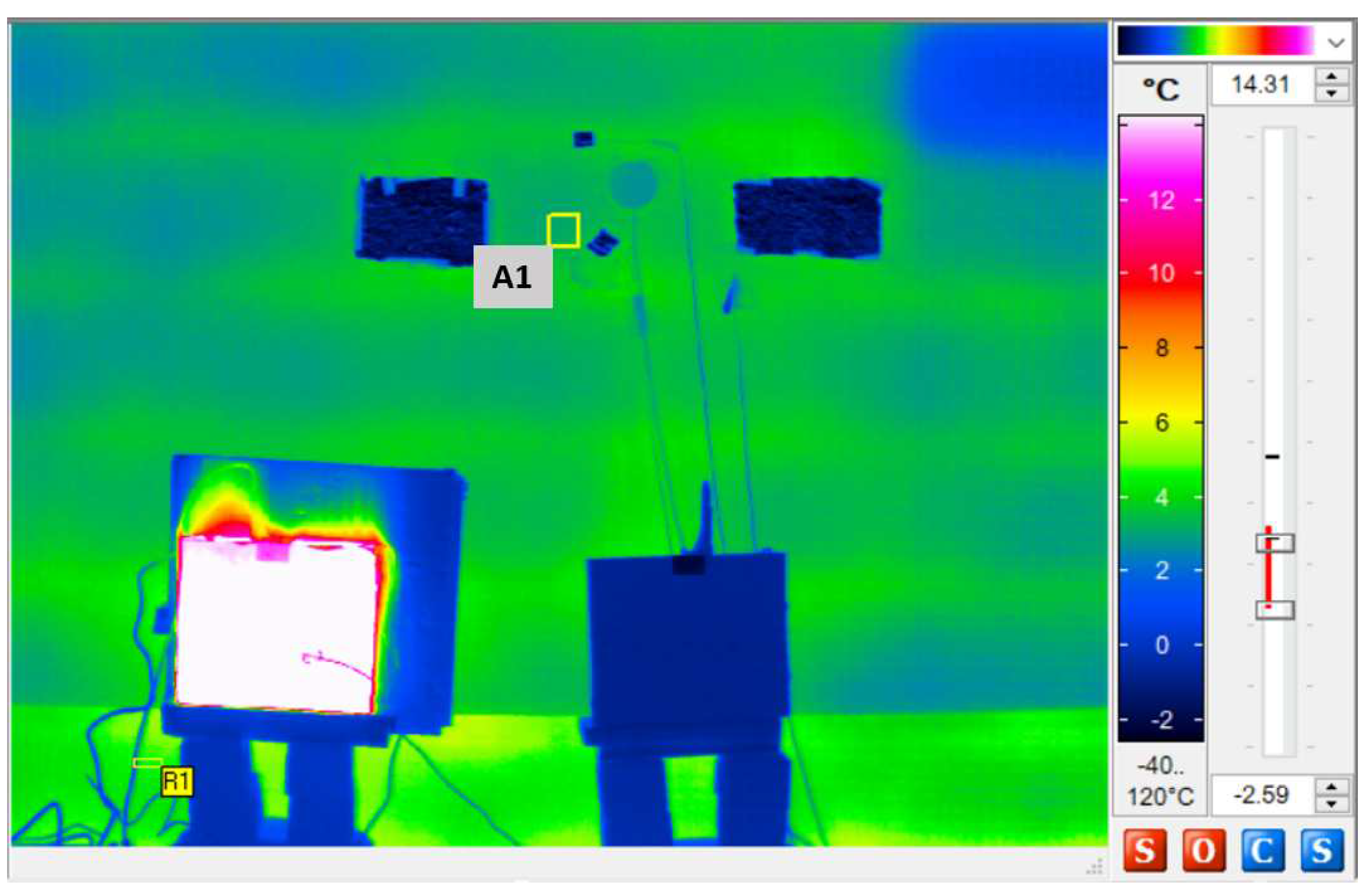
Figure 6.
Time series of corrected IR camera readings and simulated surface temperatures for a period of five consecutive days for the experiment at the test walls after optimization of wall resistance and capacitance values.
Figure 6.
Time series of corrected IR camera readings and simulated surface temperatures for a period of five consecutive days for the experiment at the test walls after optimization of wall resistance and capacitance values.
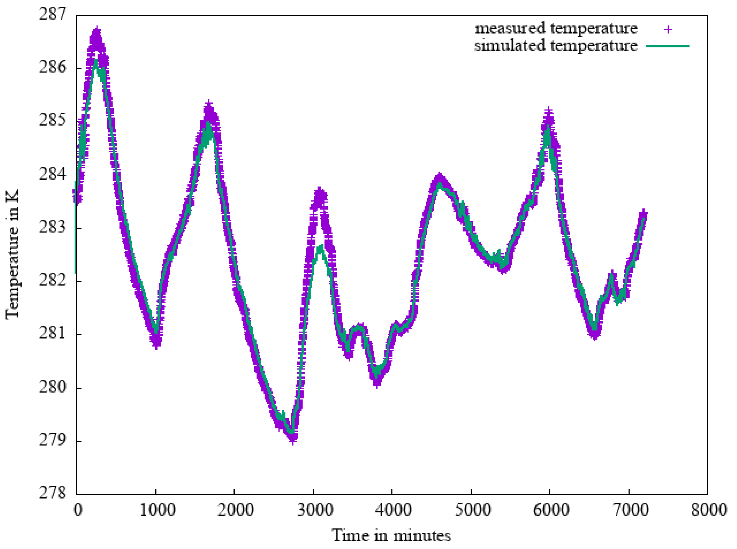
Figure 7.
Mean value (left) and standard deviation (right) of the thermal resistance for sample sizes of 10 to 1000.
Figure 7.
Mean value (left) and standard deviation (right) of the thermal resistance for sample sizes of 10 to 1000.
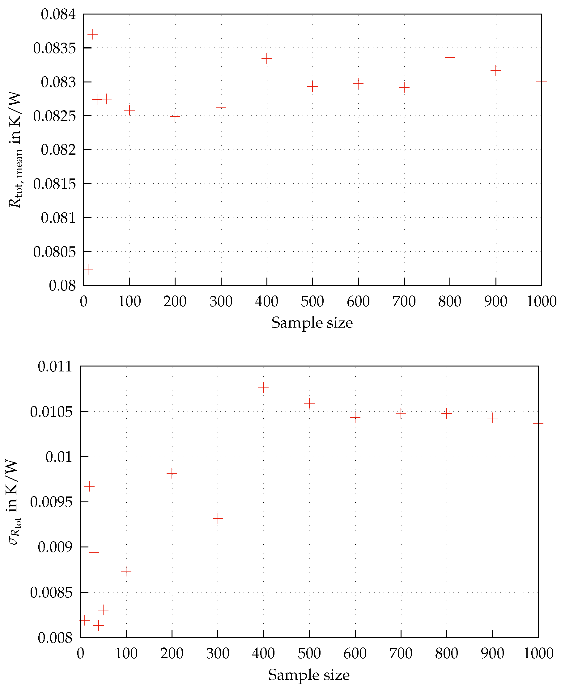

Table 1.
Results of the model calibration for the thermal resistance and the U-value using different time periods.
Table 1.
Results of the model calibration for the thermal resistance and the U-value using different time periods.
| Days | Deviation from | ||||
| 1 – 5 | 0.085 | 1.47 | 13.2 | 0.04 | 1.53 |
| 1 – 3 | 0.083 | 1.51 | 15.4 | 0.04 | 1.39 |
| 2 – 4 | 0.086 | 1.46 | 12.6 | 0.03 | 1.83 |
| 3 – 5 | 0.087 | 1.44 | 11.7 | 0.02 | 1.65 |
| 1 | 0.081 | 1.55 | 17.8 | 0.05 | 1.22 |
| 2 | 0.085 | 1.47 | 13.3 | 0.01 | 1.88 |
| 3 | 0.086 | 1.46 | 12.8 | 0.01 | 1.11 |
| 4 | 0.088 | 1.41 | 9.8 | < 0.01 | 1.9 |
Table 2.
The errors of the input quantities for the model calibration. The second column shows the source of the signal.
Table 2.
The errors of the input quantities for the model calibration. The second column shows the source of the signal.
| Quantity | Source | Error |
|---|---|---|
| Outside | NTC Sensor | |
| Outside | IR camera | |
| Outside | IR camera on aliminium foil | |
| External h | Nusselt number correlation | |
| Literature [29,30,31] | ||
| Inside | NTC Sensor | |
| Inside | NTC Sensor | |
| Internal h | Literature [32] |
Disclaimer/Publisher’s Note: The statements, opinions and data contained in all publications are solely those of the individual author(s) and contributor(s) and not of MDPI and/or the editor(s). MDPI and/or the editor(s) disclaim responsibility for any injury to people or property resulting from any ideas, methods, instructions or products referred to in the content. |
© 2023 by the authors. Licensee MDPI, Basel, Switzerland. This article is an open access article distributed under the terms and conditions of the Creative Commons Attribution (CC BY) license (http://creativecommons.org/licenses/by/4.0/).
Copyright: This open access article is published under a Creative Commons CC BY 4.0 license, which permit the free download, distribution, and reuse, provided that the author and preprint are cited in any reuse.


