
Submitted:
15 July 2023
Posted:
17 July 2023
You are already at the latest version
Abstract
Lunar seismology is a critical area of research, providing insights into the Moon's internal structure, composition, and thermal history, as well as informing the design of safe and resilient habitats for future human settlements. This paper presents the development of a state-of-the-art, three-axis broadband seismometer with a low frequency range of 0.001-1 Hz and a target sensitivity over an order of magnitude greater than previous Apollo-era instruments. The paper details the design, assembly, methodology and test results. We compare the acceleration noise of our prototype and commercial seismometers across all three axes. Increasing the test mass and reducing its natural frequency may further improve performance. These advancements in seismometer technology hold promise for enhancing our understanding of the Moon's and other celestial bodies' internal structures, and for informing the design of future landed missions to ocean worlds.
Keywords:
lunar seismology
; instrumentation
; seismometer
; planets
; space
1. Introduction
Lunar seismology has long been a subject of fascination and intrigue, not only for its scientific value but also for its implications on future human exploration and habitation of the Moon. Since the deployment of seismometers during the Apollo missions in the late 1960s and early 1970s, our understanding of the Moon's seismic activity and interior structure has evolved significantly [1,2,3]. However, many questions and challenges still remain, warranting further investigation and development of novel techniques to advance our knowledge of Earth's natural satellite.
The primary goal of lunar seismology is to decipher the Moon's internal structure, composition, and thermal history, which in turn can provide insights into the processes that have shaped its geological evolution [4]. Additionally, a comprehensive understanding of lunar seismic activity is crucial for designing and constructing safe, resilient lunar habitats for future human settlements [5,6]. In recent years, renewed interest in lunar exploration has brought forth innovative approaches to studying lunar seismology, including the development of advanced seismometers and the application of data analysis techniques adapted from terrestrial seismology [7].
These advancements have not only deepened our understanding of the Moon's seismic activity and interior structure but also paved the way for the development of more sensitive and sophisticated instrumentation. One such innovation is the prototype two-horizontal-axis broadband seismometer for lunar applications, which our group developed under NASA’s Planetary Instrument Definition and Development Program (PIDDP).
Building on this groundwork, as part of the Maturation of Instruments for Solar System Exploration (MatISSE) program, our team developed a three-axis broadband seismometer with a very low frequency range of 0.001–1 Hz and a sensitivity of at least 2 × 10⁻¹⁰ m s−2 Hz−1/2 at 1 mHz [8]. This seismometer aims at a sensitivity over an order of magnitude greater than those deployed during the Apollo era and is intended for deployment as part of a Lunar Geophysics Network (LGN) or mission to an icy Ocean World [9,10,11,12].
The over ten-fold enhancement in seismometer sensitivity across a bandwidth ranging from 1 mHz to 1 Hz enables the detection of remote teleseisms, examination of the Moon's seismic background noise, and the potential identification of the Moon's normal modes, such as the most pronounced spheroidal oscillation, 0S2, within the 8-12 mHz range [1,13]. These advancements will considerably improve the resolution of models of the Moon's and other celestial bodies' internal structures, thereby enriching our comprehension of their geological, thermal, and chemical composition [14,15,16].
The inner structures of ocean worlds, both shallow and deep, continue to be inadequately determined. A seismology experiment employing our advanced seismometer in a future landed mission could offer crucial insights into their planetary development. Through seismic monitoring of the subsurface, we can potentially identify fluid movement in the shallow layers, seismic signals originating from cryovolcanoes, and perhaps even sub-glacial ocean circulation [17].
In this article, we report the development of our MatISSE Planetary Broad-Band Seismometer (PBBS), carried out at the University of Maryland. We summarize the design and construction of our second prototype (PT-2), emphasizing the primary mechanical procedures involved in building the sensor head. We then discuss our procedure for test mass alignment and centering, and present the test results of our three-axis PT-2 seismometer. Finally, we determine the Brownian motion noise level of the instrument. We show that, by replacing the test mass with one made with a higher-density material, PT-2 should be able to meet the LGN target sensitivity over the entire frequency range of 1 mHz to 1 Hz.
2. Design and Construction
A comprehensive description of the hardware and its operating principle has been given in Reference [18]. In this section we summarize the transducer and circuit scheme. We also detail the sensor head construction, specifically the capacitor electrodes utilized for Displacement Capacitance Sensing (DCS) and Electrostatic Frequency Reduction (EFR).
2.1. Seismometer Overview
The operational principle of a seismometer entails a mass-spring system characterized by an elastic or gravitational restoring force, as illustrated in Figure 1(a). The three axes employ the same principles. Electrodes are strategically placed in the vicinity of the test mass to detect the displacement induced by ground motion. For sensing purposes, a DSC scheme is employed. Capacitors Ci1 and Ci2, where i (= x, y, z) labels the axes, form coupled pairs situated on opposite sides of the test mass. They are part of an LC bridge circuit that is driven by a frequency generator oscillator, as shown in Figure 1(b). The seismic signal at frequency ω generates two sidebands at ωpx ± . The sensed signal is subsequently decoded using a digital lock-in amplifier.
The LC bridge employs AC coupled drive and detection to minimize errors arising from the non-ideal transformer. Capacitors C11 and C10 provide AC drive coupling to the TM and permit the DCS (Cx1 and Cx2) electrodes to float. Subsequently, the C12 and C13 capacitors work in tandem to provide the DCS signal with reference to ground. While this circuit design deviates from conventional approaches, it exchanges errors associated with the transformer for requiring a higher drive voltage. The drive voltage can be commanded over a wide range which allows compensating the loss from capacitive coupling of the output by increasing the low impedance drive voltage. Notably, the ultimate sensitivity of the DCS is limited by the JFET amplifier input noise, rather than the drive amplitude.
In order for the instrument to become more sensitive at low frequencies, capacitors CNj (where j = 1-6) are utilized for electrostatic frequency reduction (EFR). By applying a high voltage between these capacitor plates and the test mass, a negative spring effect is created, which effectively counteracts the effects of the positive elastic or gravitational spring, thereby significantly reducing the natural frequency to approximately zero.
Figure 2 presents an illustration of the internal hardware configuration within the vacuum can. The spring suspension system is constructed using a triangulated structure, which consists of three aluminum (Al) triangulated pillars that support spring clamps positioned at the vertices of a titanium (Ti) triangle at the top. These spring clamps serve as connection points for the three top straight ends of the springs. The triangulated structure, along with three motors, is securely attached to a cantilever spring ring, which is mounted on the top of the sensor head.
Within the sensor head, the cylindrical test mass is enclosed, occupying a space that allows for only a 0.25 mm margin. The test mass is firmly connected to a ring using four perpendicular screws, and this ring serves as the attachment point for the other three bottom straight ends of the springs. The inner motors enable movement that can lift and tilt the test mass, while an additional three outer motors are utilized to adjust the horizontal position of the test mass by tilting the whole instrument.
2.2. Gap spacing construction
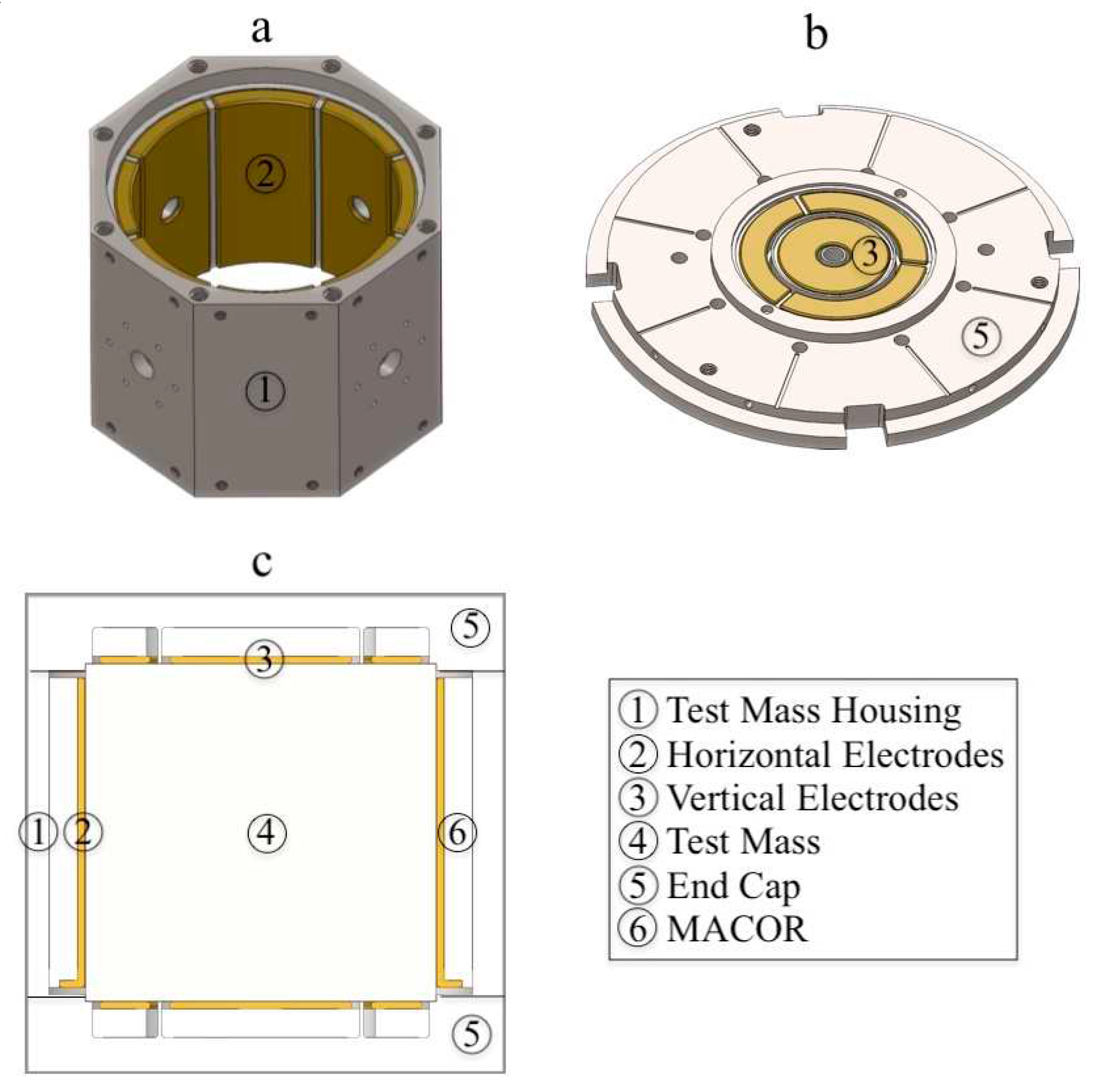
The horizontal electrodes comprise eight segmented cylindrical shells, 1 mm apart from each other. The electrodes were held together by a 1-mm thick inner non-segmented cylindrical shell, built in a single brass piece, not shown in figure 3. The part was affixed to an insulating MACOR® cylindrical shell, which was then attached to a Ti housing. Precise clearances and Teflon stoppers were strategically placed to control glue flow. Epotek® 301-2 2.5 GM low-viscosity epoxy was used, with a 3-hour curing time at 80°C. Post-assembly cleaning was required. EDM (Electrical Discharge Machining) was employed for the final step, removing the non-segmented inner brass shell to create electrically isolated, segmented shells with the inner diameter larger than the outer diameter of the test mass by 0.25 mm. All the stoppers were then removed.
The eight electrodes (figure 3a) formed four pairs of sensors and actuators. Each diametrically opposite electrodes formed a pair. Two pairs of DCS electrodes were oriented perpendicular to each other, with each pair aligned along one of the horizontal axes. The other two pairs of EFR electrodes were also perpendicular to each other but rotated 45 degrees from the DCS electrodes about the vertical axis.
The production of the end caps (figure 3b) followed a similar procedure. The three segmented DCS electrodes and the inner EFR electrode were glued one at a time, with parallelism achieved by milling the exposed electrode faces together with parts of the Ti cap at the same cutting depth. After removing the excess material from the faces of both the Ti cap and the electrodes, the resulting cavity height, exceeded the test mass height by 0.25 mm when the top and bottom caps were assembled to the housing. Strategic machining of the contact surface between the housing and end caps also enables control over perpendicularity, parallelism, and cavity height.
Although bumpers were initially considered to prevent short-circuits when the test mass contacted the electrodes, they proved unnecessary in practice. However, subsequent inspection revealed spot welding marks on the vertical electrodes, likely caused by high EFR electrical discharge in the gap spacing. No additional significant damage that might jeopardize the electrical integrity of the circuitry was observed. Electrical connections with the printed circuit boards (PCBs) on the end caps' outer surface were facilitated by spring-loaded probes that contacted the electrodes through holes in the MACOR® insulator and Ti end caps.
The springs suspending the test mass were manufactured out of non-sag doped tungsten (W) by Union City Filament Corp. Tungsten was chosen for its low thermal expansion coefficient and low internal friction [19].
Figure 3.
Perspective and cross-sectional views of the Ti housing and end caps. The Ti test mass is also shown inside the Ti housing.
Figure 3.
Perspective and cross-sectional views of the Ti housing and end caps. The Ti test mass is also shown inside the Ti housing.
3. Experimental Test
3.1. Setup
Figure 4a shows the experimental setup for PT-2, featuring two PT-2 units, although only one is functional. The other unit consists solely of the vacuum can, without the seismometer hardware. Both units share the same vacuum plumbing, with an ion pump installed in a central vacuum valve. Indium served as the sealant for most joints, while rubber O-rings were retained for coaxial cable connectors, as the experiment was performed at room temperature. The resulting pressure achieved was approximately 1 µtorr.
To measure pressure and temperature, a sensor device (SensorPush®) was positioned atop the operational seismometer. To minimize atmospheric fluctuations, an insulating thermal Styrofoam box was constructed and placed over the hardware. The box effectively mitigated short-term atmospheric variations, but was unable to counteract more pronounced long-term fluctuations. Nonetheless, it effectively suppressed sharp and fast changes.
All electronic components were supplied by our collaborator at Austin Sensors (see figure 4b). The provided equipment included two electronic boxes, cables, a monitor, a computer, and a power supply. One box housed three Field-Programmable Gate Arrays (FPGAs) and three Raspberry Pis (RPIs), one per axis. The other contained PCBs for DCS, EFR, and general monitoring, assembled on a motherboard. The majority of components were available in triplicate, one for each axis. The boxes were electronically connected via cabling between the seismometer and the computer. Austin Sensors also developed user-friendly Python software and documentation, which are stored on a local disk.
Two STS-2 seismometers and a REFTEK RT130 data logger were borrowed from the Carnegie Institute and operated concurrently with the PT-2.
3.2. Procedure for centering
A significant challenge in the experiment involved freeing and centering of the test mass relative to the surrounding sensing electrodes. The gap spacing formed between the test mass and electrodes was a mere 0.125 mm, while the perpendicular surface dimensions facing the gap were 5 cm × 5 cm, yielding a 1:400 ratio of gap spacing to surface dimension.
The process of freeing the test mass from contact with an electrode and achieving even spacing from all electrodes was accomplished through a two-phase procedure, involving EFR in both off and on states.
The procedure entailed a visual approach followed by an electronic approach when EFR was off, and fine-tuning adjustments when EFR was on.
During the visual approach, with the vacuum can open and the sensor head exposed, the spring height was adjusted by using screws at the spring clamp points. This allowed for the test mass to be suspended by the springs, and subsequently, its position to be assessed and adjusted to avoid contact with the electrodes. The inner and external motors help position the test mass, ensuring freedom of movement and approximate centering. The combination of mechanical and electronic adjustments facilitated the initial iteration of the process, with the test mass rotational mode observed to decay over a period of approximately five minutes. Modes affecting the gap spacing, such as vertical, horizontal, and rocking modes, were significantly damped and not observable due to atmospheric pressure in the gap.
Upon sealing and evacuating the vacuum can, fine-tuning was conducted exclusively through electronic means. The test mass parallelism concerning the capacitor plates was achieved by executing a computer calibration script involving the six segmented vertical sensing electrodes. The calibration script was run each time the test mass was moved vertically by the internal motors to evaluate centering relative to each segmented electrode pair, positioned at the top and bottom. If the test mass is properly centered, an EFR voltage exerts equal and opposite forces on the test mass from the two opposing capacitor plates. Therefore, changing the EFR voltage will not cause the test mass to move. On the other hand, if the test mass is not centered, a change in the EFR voltage will cause the test mass to move to a different location. Hence, the objective of the centering mechanism is to move the test mass to a location where its displacement, as indicated by the DCS, does not change when the EFR voltage is altered. This position differed from the DCS center due to mismatch in the stray capacitance. Using these processes, the frequency was successfully reduced from 2.89 Hz to 0.5 Hz.
With the vertical axis configuration maintained at 0.5 Hz or slightly higher, the EFR was next applied to the horizontal axes. Due to complexities in working with two axes in the horizontal plane, the test mass could not be positioned at the EFR center. Consequently, the horizontal axes were centered to the DCS center by using the external motors. Gradual and non-isotropic EFR application enabled the reduction of the two horizontal modes from 1.5 Hz to 0.5 Hz. High quality factors observed in all three directions indicated that the test mass was successfully freed.
4. Data Analysis
4.1. PT-2 transfer function
The STS-2 seismometer exhibits a flat response between 120 s and 50 Hz, with ground motion velocity data derived through a multiplicative factor applied to the raw data [20,21]. Acceleration noise is subsequently calculated using a derivative calculus procedure on the velocity dataset. As the PT-2 response to ground motion has not been experimentally determined, a theoretical derivation is employed using Eq. (5) from reference [22]. This equation presents the transfer function for a mass-spring system:
where b represents a parameter determining the system's viscous damping, considered null (b = 0) in our case. ωs and ω0 denote the system's natural and reduced frequency, respectively. According to Eq. (12) in another reference [23], the loss angle due to the spring's internal friction can be expressed as a function of the quality factor Qi associated with that channel:
Substituting Eq. (2) into Eq. (1) yields the transfer function in terms of the quality factor computed when PT-2 is operated at the reduced frequency ω0:
The ground motion acceleration noise, presented in the next section, is determined by multiplying the transfer function by the PSD of the test mass displacement raw data obtained from the experiment.
4.2. Power spectral densities
Figure 5 presents data plots derived from all three axes, with EFR applied simultaneously. Each axis had a sample rate of 250 samples per second, which was the same as that of the STS-2 one. The DCS drive amplitude was set to 0.15 V. The first column displays the x-axis spectrum and time series for both the PT-2 and STS-2. A cluster of peaks ranging from 0.46 Hz to 0.54 Hz is observed, potentially attributable to frequency drift and closely positioned horizontal modes. We employed the average frequency in the transfer function, suppressing the 0.5-Hz frequency peak with a Q-factor of approximately 150. Additional peaks near 1 Hz and 0.1 Hz are visible, possibly resulting from axes crosstalk and ground motion, respectively. The y-axis spectrum bears similarities to the x-axis spectrum, save for an isolated peak at approximately 27 mHz, which might also stem from crosstalk.
The z-axis component spectrum exhibits poor agreement with the STS-2 spectrum at frequencies below 86 mHz, where the PT-2 acceleration noise was 5.8 × 10⁻⁸ . The STS-2 minimum noise occurred at 39 mHz with a value of 1.05 × 10⁻⁸ . This discrepancy amounts to a factor of roughly 5.5 between PT-2 and STS-2 at low frequencies. Due to data filtering, the time series of all three axes did not display significant displacement drift during the examined data set period, which is a segment of a 24-hour-long data collection run, characterized by reasonable test mass stability before eventual collapse. As predicted by our EFR theory, the test-mass energy potential well is relatively shallow at this frequency level, rendering the test mass prone to lose stability, by escaping the potential well due to environmental noise driven kinetic energy.
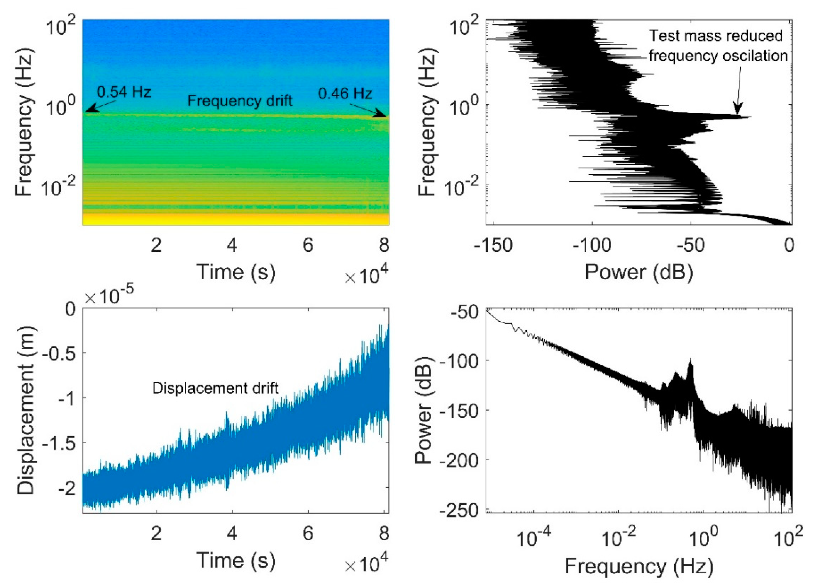
Figure 6 presents the spectrogram of test mass displacement for the vertical axis alongside the unfiltered displacement data as a function of time, corresponding to the filtered data depicted in figure 5. Additionally, the power of displacement and frequency are plotted against each other. The unfiltered displacement graph clearly reveals drift over time. In the spectrogram, it is evident that the entire spectrum, from the pendulum frequency of about 0.5 Hz downward, originates from a continuous signal. No distinct signals, such as a chirp—which may result from an earthquake—are observable within this time window.
The bottom left quadrant highlights the observable drift in displacement, while the top left quadrant concurrently illustrates the corresponding drift in frequency at around 0.5 Hz. The observed drift is likely a result of the combined effects of temperature drift and spring creep. However, no specific measurements have been conducted to ascertain the magnitudes of both factors at present.
4.3. Dynamic range
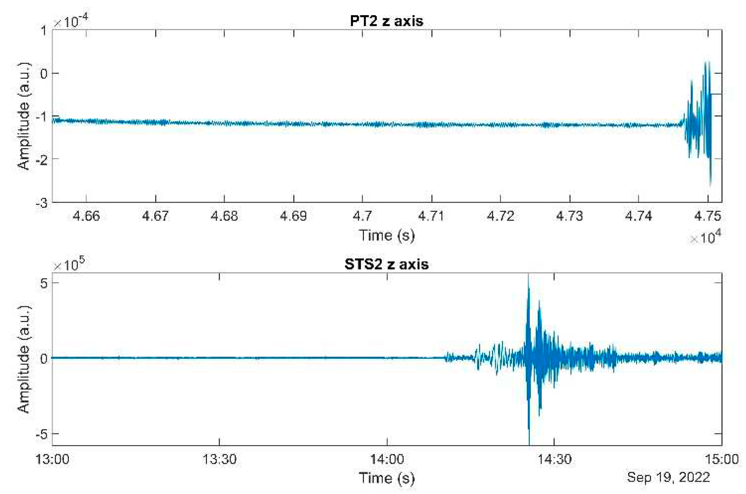
On September 19, 2022, pronounced oscillations were observed in real time on the PT-2 monitor screen. Upon investigating the signal on STS-2, it was confirmed that the signal represented genuine ground motion. See figure 7. This event corresponded to a magnitude 7.6 earthquake off the Western Coast of Mexico, according to data available on the referenced website [24]. Due to the lack of a dynamic range implementation at the time, PT-2 could not record the entire signal duration as STS-2 did. The test mass lost stability while EFR was active and become latched on the electrodes.
Figure 7.
Earthquake detection data from the PT-2 and STS-2 instruments, collected on September 19, 2022. The upper panel presents the response of the PT-2 z-axis test mass displacement, while the lower panel depicts the ground motion velocity recorded by the STS-2 z-axis. Notably, the PT-2 instrument's data for the entire earthquake event is absent, attributable to its limited dynamic range at the time. The PT-2 data have been truncated on the left side since it does not align with the scenario when the test mass is in a free state.
This incident prompts a discussion on the potential incorporation of dynamic range mechanisms. EFR application reduces the frequency to enhance sensitivity at lower frequencies, allowing the detection of moonquakes with minimal amplitude at these frequencies. However, if the moonquake amplitude is sufficiently high, enhanced sensitivity is no longer required for detection. Consequently, it is feasible to deactivate EFR when the dynamic range is about to be exceeded, providing effectively a path for implementing a high dynamic range.
5. Brownian Motion Noise for the Vertical Axis
Part of the Brownian motion noise arises from spring internal friction. Although the current performance of the PT2 vertical sensor is not solely limited by the Brownian motion noise of the suspension spring, it is the ultimate and more stringent among all noises. We now explore potential strategies to mitigate the Brownian motion noise. A formula presented in [22] defines the Brownian motion acceleration noise for a mass-spring oscillator as
where , m = 0.465 kg; ks = 152 N/m; T = 293 K; kB = 1.380649 x 10⁻²³ m2 kg s-2 K-1. The loss angle (ɸ) is material-dependent and can be found by using the EFR technique [23]. A formula involving the quality factor and the reduced frequency is given by Eq. (2):
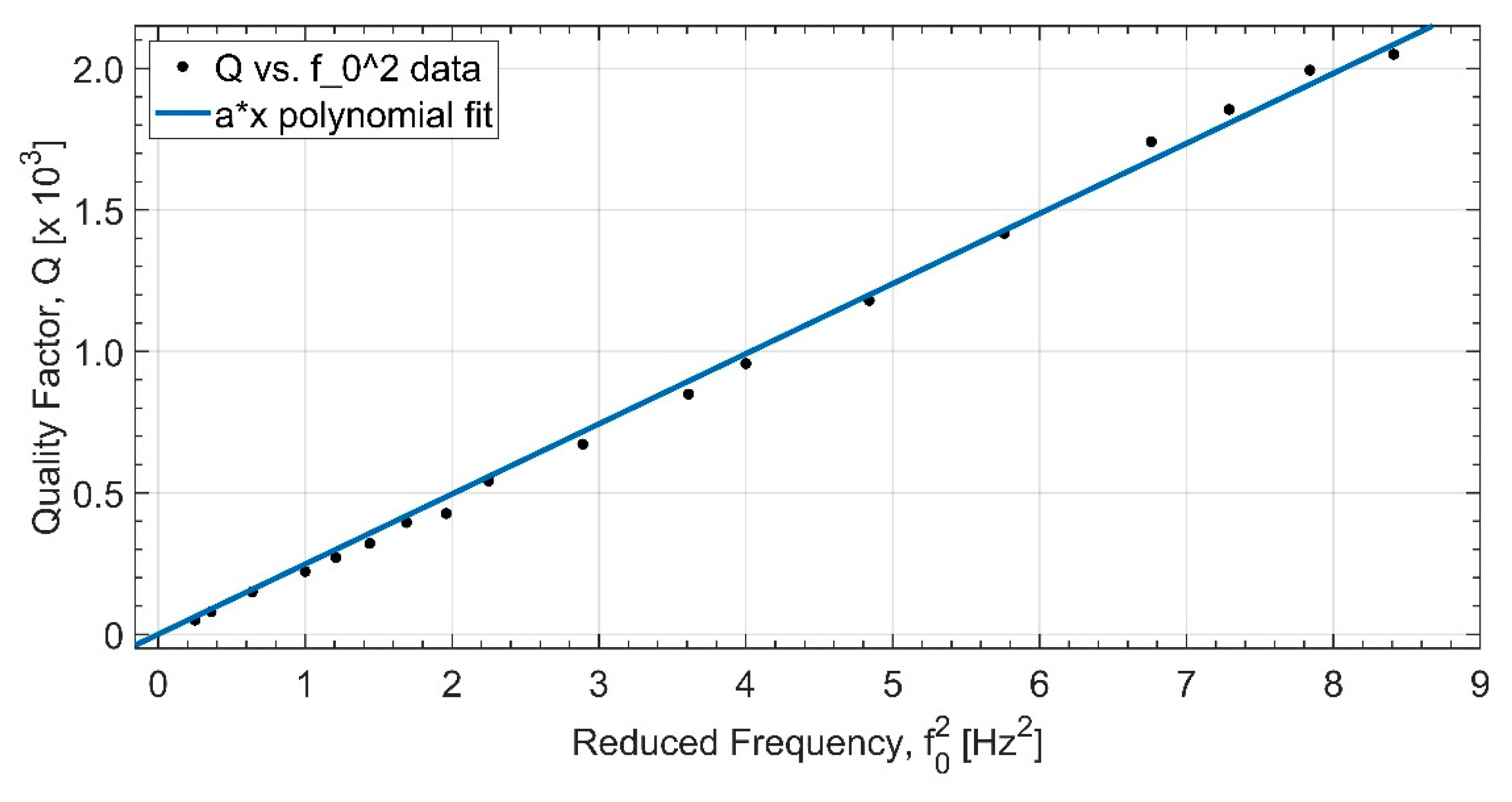
Experimental data for Q values are plotted against in figure 8. A linear fit to the data yields
From this, we get the loss angle:
Substituting Eq. (7) into Eq. (4), we calculate the Brownian motion noise for the vertical axis at f = 1 mHz for two different sets of T and m:
- At earth room temperature T = 293 K, m = 0.465 kg (Ti): 9.32 × 10⁻¹⁰ m s-2 Hz-1/2;
- At lunar night-time temperature T = 140 K, m = 1.5 kg (Cu25-W75): 2.0 × 10⁻¹⁰ m s-2 Hz-1/2.
Figure 8.
Experimental data for the Q factor are plotted against reduced frequency squared for the vertical axis.
Figure 8.
Experimental data for the Q factor are plotted against reduced frequency squared for the vertical axis.
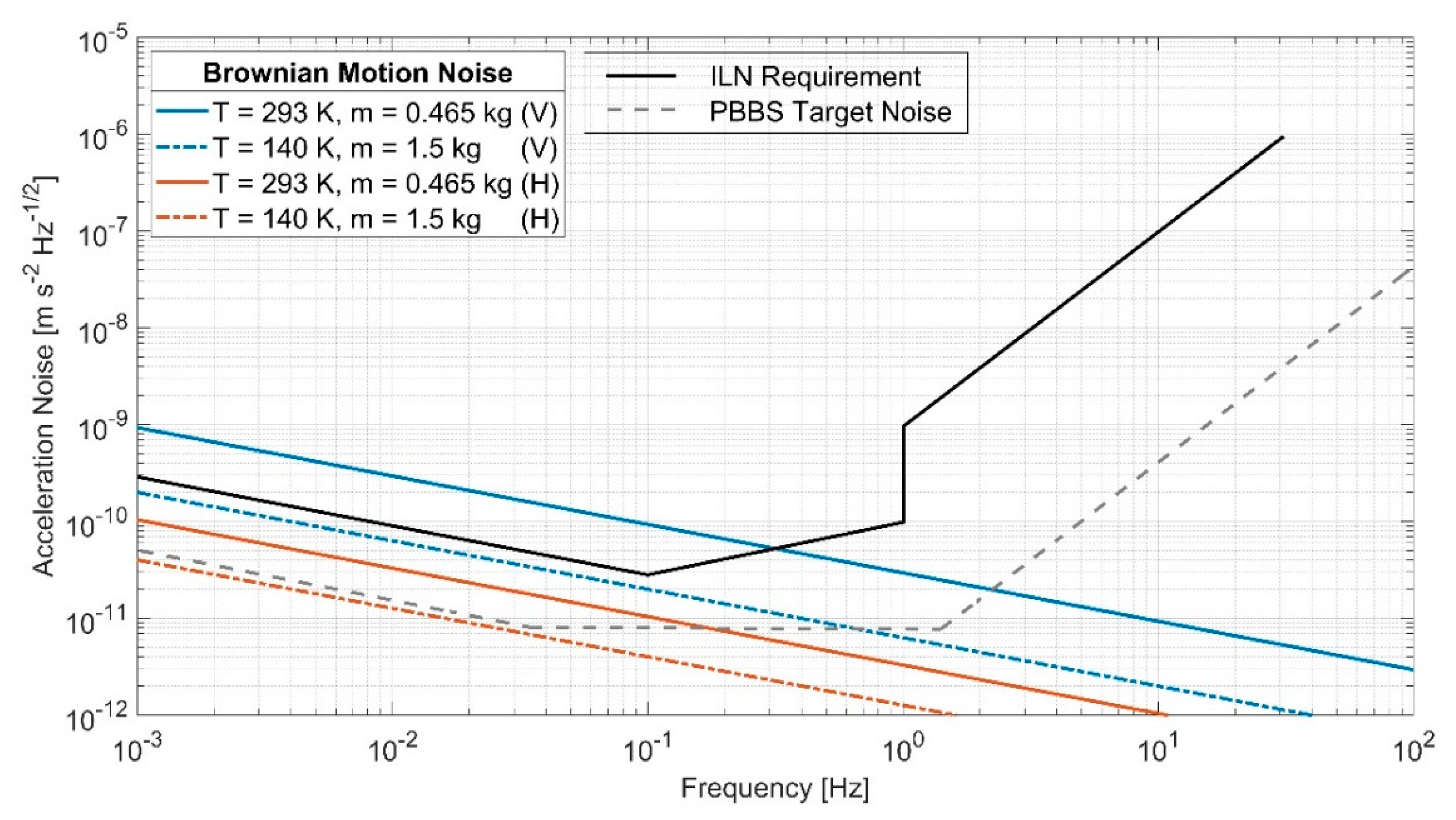
We can see that, if the mass is increased from the present value, 0.465 kg, to m = 1.5 kg (by changing the test mass material from Ti to copper-tungsten), PT-2 could meet the stringent ILN requirement of 2.0 × 10⁻¹⁰ m s–2 Hz–1/2 at 1 mHz, as shown in figure 9. Furthermore, the Brownian motion noise associated with the horizontal axes is lower than that for the vertical axis. This is because, for the horizontal axes, the stiffness is provided by gravity potential and EFR, which are both frictionless. There is only a small coupling to the internal damping of the spring material through the bending of the suspension spring near the suspension point [25]. Substituting the design parameters of our tungsten spring into Eq. (21) of [25], we obtain a dilution factor of 0.05 for damping, which leads to the estimated effective loss angle for PT-2 horizontal of , which was used to estimate the horizontal Brownian motion noise level.
Figure 9.
Comparative analysis of noise levels between the Brownian motion and the specifications set by the International Lunar Network (ILN). The figure shows two distinct configurations for both vertical and horizontal axes, based on varying temperature and mass parameters. The use of a test mass of 1.5 kg on the lunar surface appears promising for mitigating the Brownian noise, thus potentially allowing the system to achieve the sensitivity levels required by the ILN. V and H are abbreviattions for vertical and horizontal axis, respectively.
6. Discussions
The spectrum for the PT-2 horizontal components exhibited two additional resonant peaks at frequencies of 27 mHz and 1 Hz. Since these peaks did not correspond to any features in the STS2 spectrum, it is likely that they originated from instrumental sources. One plausible explanation is a potential disparity between the x and y axis FPGA clocks, which could generate slightly different drive frequencies and lead to crosstalk. However, the clocks have been replaced, and a more viable explanation is that these peaks were a result of the subtraction and addition of the two horizontal modes due to non-linearities. We attempted to anisotropically adjust the horizontal EFR voltages in order to bring down the two horizontal modes from 1.5 Hz to approximately 0.5 Hz. Nevertheless, when these modes approached proximity, they could couple and give rise to split modes separated by 20 mHz around 0.5 Hz. This phenomenon could account for the presence of the additional two peaks through the subtractive and additive interactions of the two original modes.
We were able to collect the data with resonance frequencies reduced to 0.2 Hz for the horizontal axes and 0.3 Hz for the vertical axis. However, as the frequency decreases, the test mass becomes more susceptible to instability. The potential well is shallower and there is an increased likelihood of the test mass latching onto the electrodes. This problem will largely be alleviated in the quiet lunar environment. The data collected with lower resonance frequencies are not yet relevant, so the presented data corresponds to the more stable case where the resonance frequencies were approximately 0.5 Hz. Better agreement with STS-2 is anticipated upon controlling the test mass at lower frequencies down to 0.01 Hz.
The spectrum of all three axes exhibited a similar 1/f noise limitation, reaching the same noise floor. This limitation in the PT-2 spectrum can be attributed to several factors. First, our inability to reliably decrease the resonance frequency from 0.5 Hz to the desired 0.01 Hz contributes to this limitation. Secondly, there may be other sources of noise, such as electronic noise, impacting the noise. In the case of an imbalanced bridge circuit, for instance, oscillator noise can arise, hindering the decoding of low-frequency sidebands. Third, the signal-to-noise ratio (SNR) is contingent upon the amplitude of the DCS drive, and the difficulty to maintain the test mass near its central position at present prevents the utilization of the maximum drive amplitude level. As a consequence, the SNR is compromised, which is likely a contributing factor to the subpar performance observed at lower frequencies.
The DCS drive utilized in the system operates at a frequency of 40 kHz and is precisely controlled by a crystal. It exhibits minimal long-term drift at the scale of seconds. The variability in phase jitter primarily stems from the SNR. Prior to delivery, the bridge was fully balanced. However, it is uncertain whether any verification was conducted subsequent to installation. It is also plausible that the system may have been operational without the phase being appropriately configured. An additional factor that can introduce nonlinearity is the overdrive of the DCS resulting from setting the amplitude too high. The cumulative impact of off-center operation, displacement, and drive amplitude contributes to this outcome.
The pressure fluctuations may have an impact on the noise. This phenomenon is widely recognized within the field of seismology. However, we regrettably did not examine the correlation between PT-2 data and the corresponding pressure measurements.
We have previously provided an extensive analysis of temperature-sensitivity-induced noise in seismometers, employing both quantitative and analytical approaches to explore the temperature dependence of a spring-suspended mass model with EFR [18]. We proposed practical solutions to minimize thermal effects on lunar seismometers by carefully selecting materials for the seismometer housing and spring suspension to balance shear modulus and thermal expansion coefficients. Our current configuration requires a distance between the top and bottom spring clamps of 105-108 mm to achieve a minimum of 99% cancellation/mitigation (Eq. (39) in the paper). This would result in a temperature sensitivity of 2 × 10⁻⁸ m K-1 and a temperature spectral density of 30 µK Hz-1/2, meeting the ILN requirement of 2 × 10⁻¹⁰ m s-2 Hz-1/2 at 1 mHz. Employing a multi-layer insulation (MLI) shield may provide adequate temperature control on the lunar surface.
7. Conclusions
We tested our MatISSE PT-2 seismometer alongside two STS-2 seismometers, and conducted a comparative analysis of acceleration noise between both instruments across all three axes. First, we applied EFR to the horizontal components while maintaining the vertical component in a suppressed state to avoid crosstalk. Second, we applied EFR solely to the vertical component. Finally, we ran all three axes concurrently, applying EFR and collecting data from all axes simultaneously. The comparison reveals that EFR can be implemented across all three axes simultaneously, and the PT-2 seismometer can operate without increased noise, barring potential electronic crosstalk or nonlinearities.
All three axes reached the same noise floor at low frequencies. Although the main cause for this remains unclear, it is suggestive that all three axes are limited by the same 1/f noise at present. The PT-2 horizontal axes displayed better noise agreement with the STS-2 than the vertical axis. However, it is important to highlight that the vertical axis of the STS-2 seismometer exhibits greater sensitivity compared to its horizontal axes.
EFR was applied to all three axes up to a reduced frequency of approximately 0.5 Hz. The observed Qs of 2,000 and 12,000 for the vertical and horizontal components indicate that the test mass was free. Although the PT-2 has yet to surpass the STS-2's low-frequency performance, operating all three axes at a reduced frequency of 0.5 Hz is considered to be an accomplishment, given the small gap spacing of 0.125 mm between the test mass and electrodes. To align with the STS-2 z-axis sensitivity, a possible solution entails lowering the EFR frequency to 0.01 Hz, which necessitates precise compensation of temperature sensitivity and exceptional test mass centering to avoid instability under high EFR voltage.
Temperature-sensitivity-induced noise relies on effective temperature compensation and control. As previously demonstrated, a noise level as low as 2 × 10⁻¹⁰ m s-2 Hz-1/2 at 1 mHz can be attained through spring height adjustments and the implementation of an MLI shield. Here the Brownian noise was calculated by using the experimental Q data. Increasing the test mass to approximately 1.5 kg by replacing titanium with copper-tungsten, while preserving PT-2's other design parameters, may suffice to reduce the Brownian motion noise to ILN-required levels.
Data Availability Statement
The data that support the findings of this study are available upon reasonable request.
Acknowledgments
We acknowledge useful discussions with Andrew Erwin, Sharon Kedar, Vol Moody, and Christopher Collins. The development of a broadband planetary seismometer with elec-trostatic frequency tuning started with the NASA PIDDP program and was subsequently funded by the NASA MatISSE program. N.C.S. was supported by NASA (Grant Nos. 80NSSC19M0216 and 80NSSC18K1628). We also thank Bruce Lee for the final machining of the seismometer housing. We are deeply indebted to the Carnegie Institute at Wash-ington D.C. for graciously lending us two STS2 units.
References
- Philippe Lognonné, Planetary Seismology, Annual Review of Earth and Planetary Sciences, v. 33(1), pp. 571-604 (2005). [CrossRef]
- N. R. Goins, A. M. Dainty, and M. N. Toksöz, Lunar seismology: The internal structure of the Moon, J. Geophys. Res. 86(B6), 5061–5074, (1981). [CrossRef]
- Y. Nakamura, G. V. Latham, and H. J. Dorman, Apollo lunar seismic experiment—Final summary, J. Geophys. Res. 87(S01), A117–A123, (1982). [CrossRef]
- R. Jaumann, H. Hiesinger, M. Anand, I.A. Crawford, R. Wagner, F. Sohl, B.L. Jolliff, F. Scholten, M. Knapmeyer, H. Hoffmann, H. Hussmann, M. Grott, S. Hempel, U. Köhler, K. Krohn, N. Schmitz, J. Carpenter, M. Wieczorek, T. Spohn, M.S. Robinson, J. Oberst, Geology, geochemistry, and geophysics of the Moon: Status of current understanding, Planetary and Space Science, v. 74(1), pp. 15-41 (2012). ISSN 0032-0633. [CrossRef]
- G. J. Taylor, P. D. Spudis, Geoscience and a Lunar Base: A Comprehensive Plan for Lunar Exploration, NASA Conference Publication 3070, (1990). https://ntrs.nasa.gov/citations/19900015714.
- The Artemis Accords, 2020, https://www.nasa.gov/specials/artemis-accords/index.html.
- Nunn, C., Garcia, R.F., Nakamura, Y. et al. Lunar Seismology: A Data and Instrumentation Review. Space Sci Rev 216, 89 (2020). [CrossRef]
- G. Latham, M. Ewing, F. Press, and G. Sutton, The Apollo passive seismic experiment, Science 165(3890), 241–250 (1969). [CrossRef]
- C. Shearer and G. Tahu, Lunar geophysical network (LGN), mission concept study, NASA, 2017, https://solarsystem.nasa.gov/studies/203/lunar-geophysical-network-lgn/.
- P. Lognonné et al, SEIS: Insight’s seismic experiment for internal structure of Mars, Space Sci. Rev. 215, 12 (2019). [CrossRef]
- E. Wielandt and G. Streckeisen, The leaf-spring seismometer: Design and performance, Bull. Seismol. Soc. Am. 72(6A), 2349–2367 (1982). [CrossRef]
- P. Lognonné et al, Seismology on Artemis III: Exploration and science goals, White paper, 2020, https://www.lpi.usra.edu/announcements/artemis/whitepapers/2030.pdf.
- A. Khan and K. Mosegaard, New information on the deep lunar interior from an inversion of lunar free oscillation periods, Geophys. Res. Lett. 28(9), 1791–1794, (2001). [CrossRef]
- Y. Nakamura, Farside deep moonquakes and deep interior of the Moon, J. Geophys. Res.: Planets 110(E1), E01001, (2005). [CrossRef]
- E. Larose, A. Khan, Y. Nakamura, and M. Campillo, Lunar subsurface investigated from correlation of seismic noise, Geophys. Res. Lett. 32(16), L16201, (2005). [CrossRef]
- P. Lognonné and B. Mosser, Planetary seismology, Surv. Geophys. 14, 239–302 (1993). [CrossRef]
- S. D. Vance et al, Geophysical investigations of habitability in ice-covered ocean worlds, J. Geophys. Res.: Planets 123(1), 180–205, (2018). [CrossRef]
- L. A. N. de Paula; H. J. Paik; N. C. Schmerr; A. Erwin; T. C. P. Chui; I. Hahn; P. R. Williamson, Temperature sensitivity analysis on mass-spring potential with electrostatic frequency reduction for lunar seismometers, AIP Advances. v 11(12), p. 125019 (2021). [CrossRef]
- Union City Filament Corp. https://ucfilament.com/.
- Streckeisen STS-2 Broadband Sensor, PASSCAL Instrument Center. Available at: https://www.passcal.nmt.edu/content/instrumentation/sensors/broadband-sensors/sts-2-bb-sensor.
- Working with Responses to Get Units of Ground Motion, PASSCAL Instrument Center. Available at: https://www.passcal.nmt.edu/content/instrumentation/field-procedures/working-responses-get-units-displacement.
- A. Erwin; L. A. N. de Paula; N. C. Schmerr; D. Shelton; I. Hahn; P. R. Williamson; H. J. Paik; T. C. P. Chui, Brownian Noise and Temperature Sensitivity of Long-Period Lunar Seismometers, Bulletin of the Seismological Society of America 111 (6), 3065–3075 (2021). [CrossRef]
- A. Erwin; K. J. Stone; D. Shelton; I. Hahn; W. Huie; L. A. N. de Paula; N. C. Schmerr; H. J. Paik; T. C. P. Chui, Electrostatic frequency reduction: A negative stiffness mechanism for measuring dissipation in a mechanical oscillator at low frequency, Review of Scientific Instruments 92(1), 015101 (2021). [CrossRef]
- M 7.6 - 35 km SSW of Aguililla, Mexico. https://earthquake.usgs.gov/earthquakes/eventpage/us7000i9bw/executive.
- G. Cagnoli; J. Hough; D. DeBra; M.M. Fejer; E. Gustafson; S. Rowan; V. Mitrofanov, Damping dilution factor for a pendulum in an interferometric gravitational waves detector, Physics Letters A 272, 39-45 (2000).
Figure 1.
(a) Mechanical configuration of capacitor plates for the two horizontal axes employed for both sensing and frequency reduction in the seismometer. The test mass is suspended using springs and is surrounded by sensors and actuator electrodes. (b) Schematic circuit diagram for DCS for the x axis. The LC resonant circuit formed by the two sensing capacitors and two equal inductors are driven by an oscillator at frequency ωpx . The amplifier output is demodulated to obtain the low-frequency seismic signals.
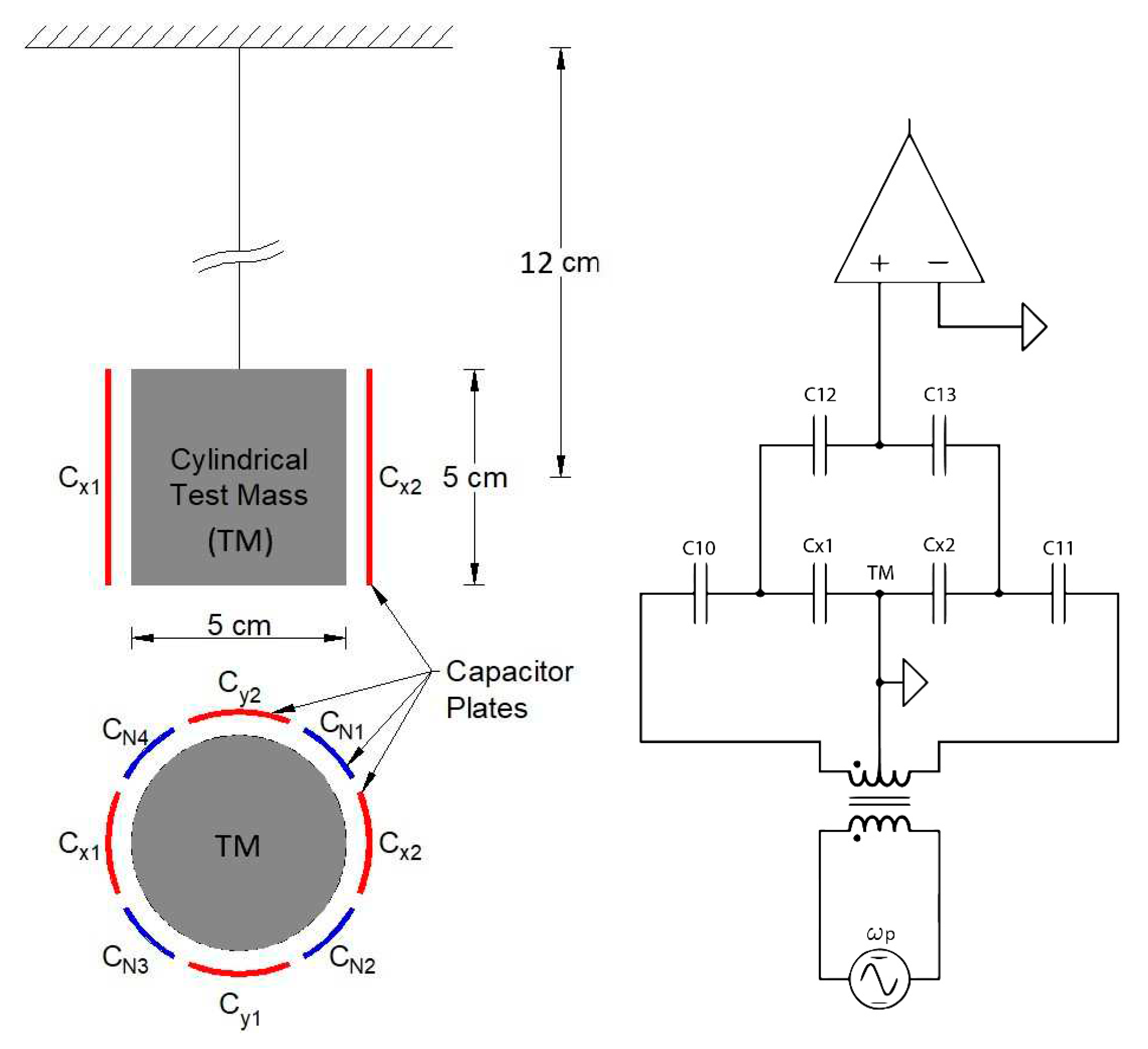
Figure 2.
A perspective view of the hardware, encompassing the sensor head, springs, suspension, motors, and the lower section of the vacuum can. Notably, the representation intentionally excludes the cover of the vacuum for clarity and simplification.
Figure 2.
A perspective view of the hardware, encompassing the sensor head, springs, suspension, motors, and the lower section of the vacuum can. Notably, the representation intentionally excludes the cover of the vacuum for clarity and simplification.
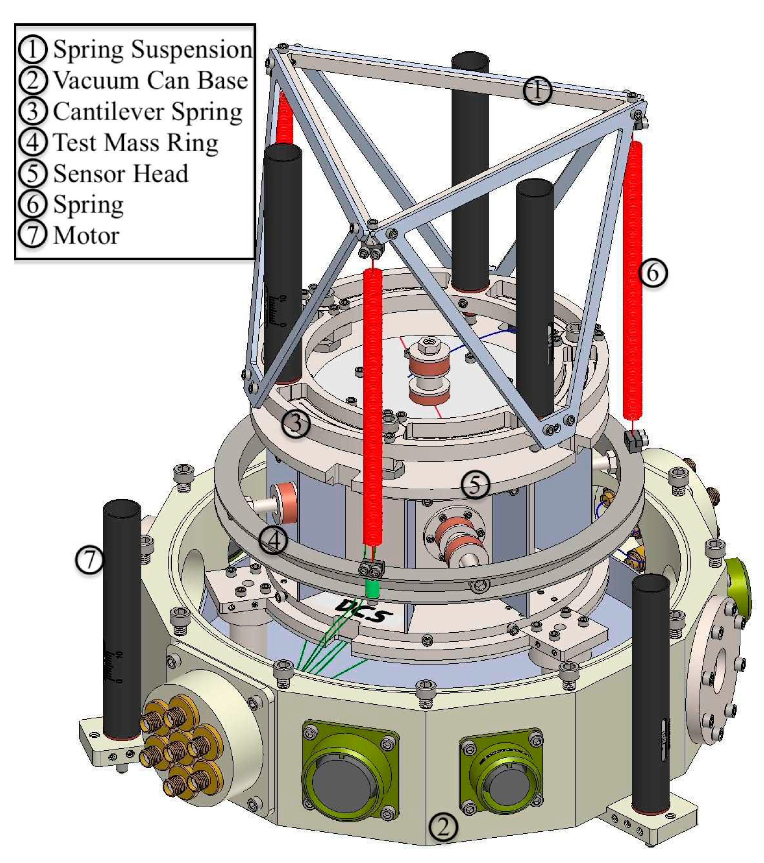
Figure 4.
a) Experimental setup showing the raised Styrofoam box, STS-2 and PT-2 seismometers, ion pump, SensorPush® and vacuum plumbing. b) Electronics rack showing the lowered Styrofoam box, power supplies, pressure gauge, EFR and FPGA boxes and ion pump controller.
Figure 4.
a) Experimental setup showing the raised Styrofoam box, STS-2 and PT-2 seismometers, ion pump, SensorPush® and vacuum plumbing. b) Electronics rack showing the lowered Styrofoam box, power supplies, pressure gauge, EFR and FPGA boxes and ion pump controller.
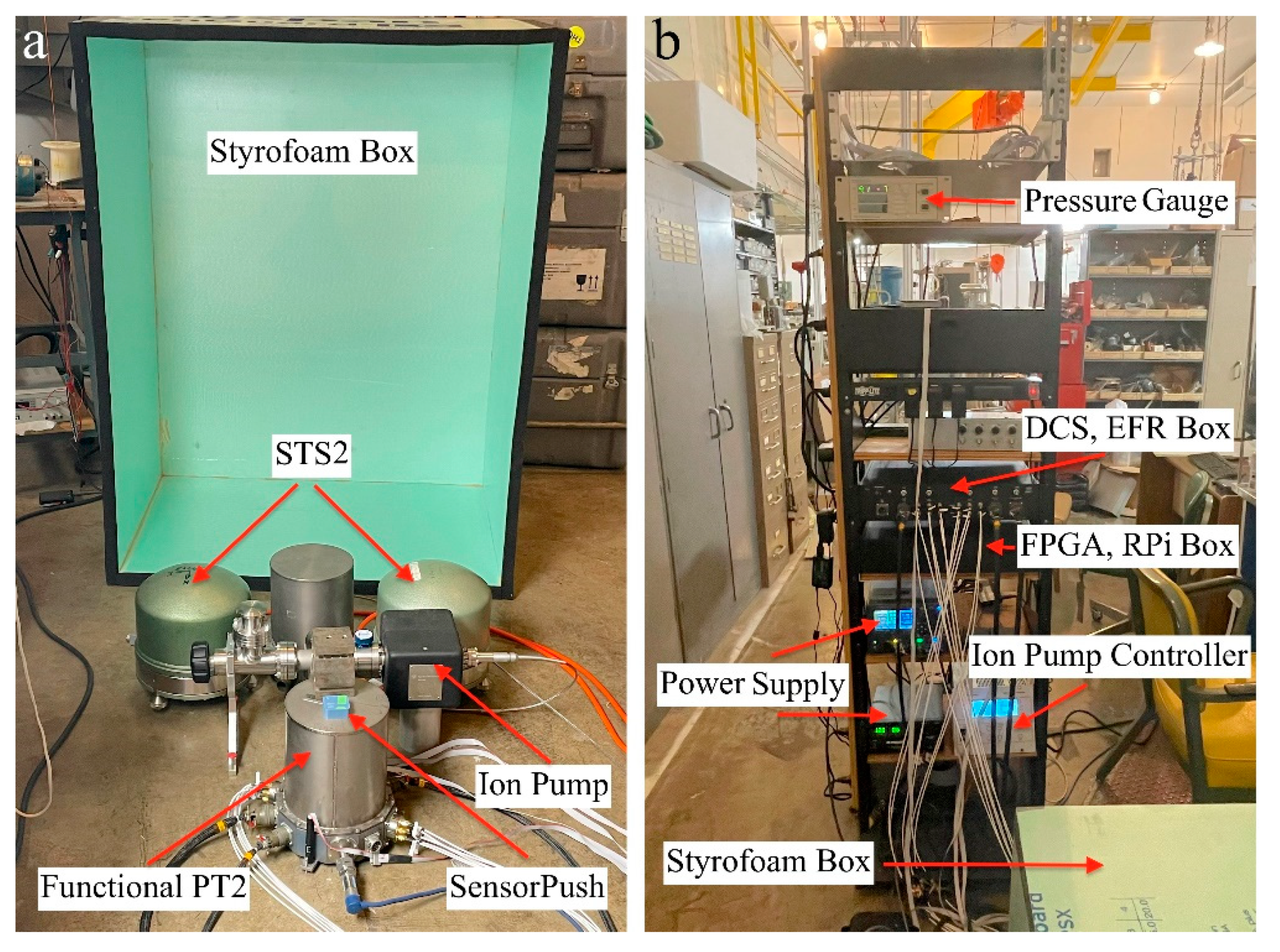
Figure 5.
Plots from data with EFR applied on all three axes simultaneously. The graphical representations are organized in a three-column format, with each column corresponding to one of the axes. In the first row, a comparative analysis of the acceleration noise spectral densities for PT-2 and STS-2 is illustrated. The second row shows the temporal evolution of test mass displacement, while the ground motion velocity time series is seen in the third row. The peak at 0.5 Hz represents the resonance frequency of the TM-spring system, while the frequencies at 27 mHz and 1 Hz account for crosstalk.
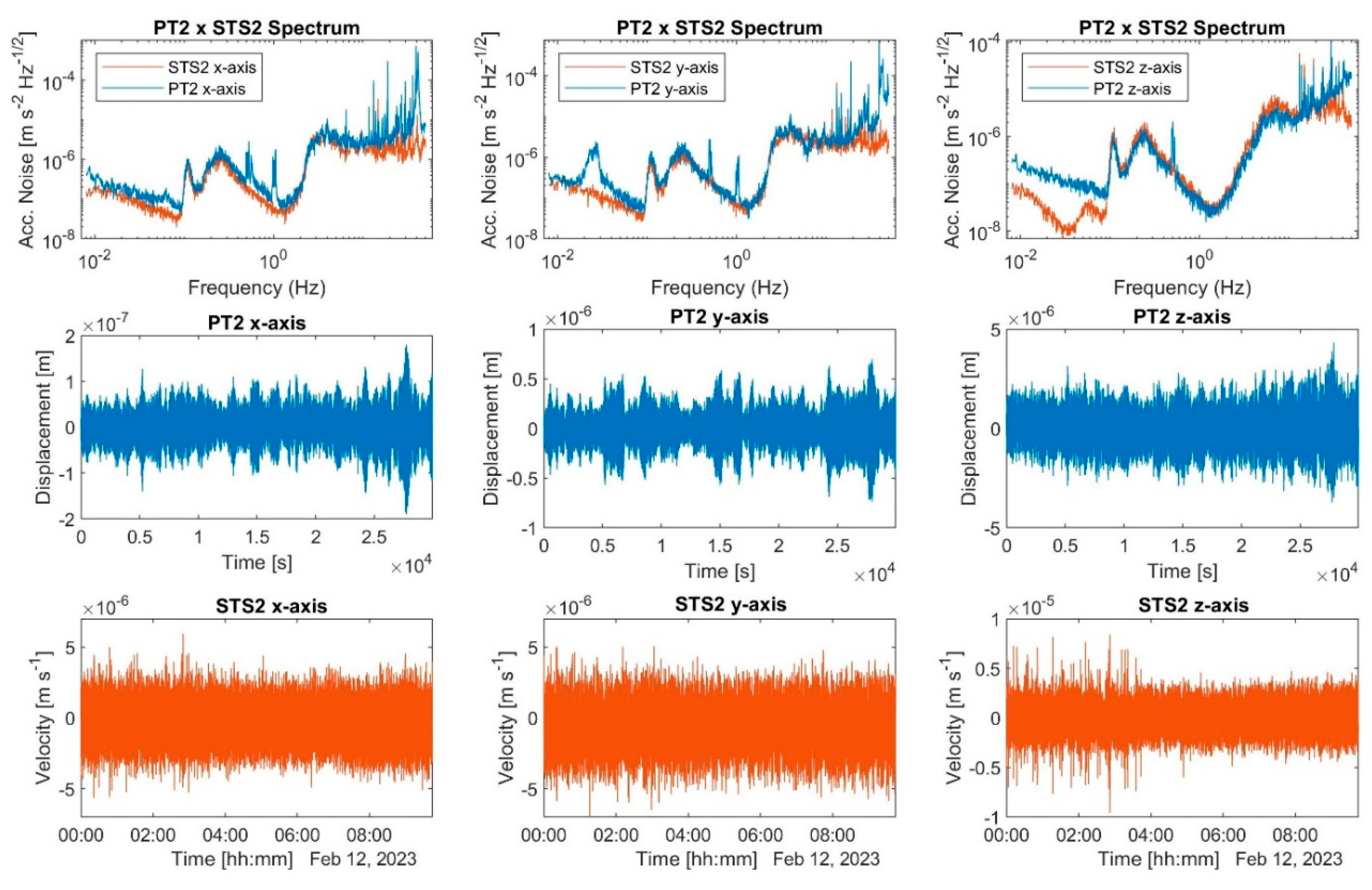
Figure 6.
The spectrogram of vertical axis is shown in the top left quadrant with three more auxiliary plots. Bottom left: the test mass displacement is presented as a time series. Top right: the reciprocal of the power of displacement as function of frequency, which is shown in the bottom right. The magnitude of the spectral lines in the top-left region of the graph can be observed by tracing horizontally towards the right, where the highest magnitudes are depicted as peak values.
Disclaimer/Publisher’s Note: The statements, opinions and data contained in all publications are solely those of the individual author(s) and contributor(s) and not of MDPI and/or the editor(s). MDPI and/or the editor(s) disclaim responsibility for any injury to people or property resulting from any ideas, methods, instructions or products referred to in the content. |
© 2023 by the authors. Licensee MDPI, Basel, Switzerland. This article is an open access article distributed under the terms and conditions of the Creative Commons Attribution (CC BY) license (http://creativecommons.org/licenses/by/4.0/).
Copyright: This open access article is published under a Creative Commons CC BY 4.0 license, which permit the free download, distribution, and reuse, provided that the author and preprint are cited in any reuse.


