Submitted:
09 July 2023
Posted:
12 July 2023
You are already at the latest version
Abstract
Electricity demand forecasting plays a significant role in energy markets. Accurate prediction of electricity demand is the key factor to optimize power generation, consumption, saving energy resources, and determining the energy prices. However, integrating energy mix scenarios, including solar and wind power which are highly non-linear and seasonal, into an existing grid increases uncertainty in generation, adds the challenges for precise forecast. To tackle these challenges, state-of-the-art methods and algorithms have been implemented in literature. We have developed Artificial Intelligence (AI) based deep learning models that can effectively handle the information of long time-series data. Based on the pattern of dataset, four different scenarios were developed and two best scenarios were selected for prediction. Dozens of models were developed and tested in deep AI networks. In the first scenario (Scenario1), data for weekdays excluding holidays was taken and in the second scenario (Scenario2) all the data in the basket was taken. Remaining two scenarios, weekends and holidays were tested and neglected because of their high prediction error. To find the optimal configuration, models were trained and tested within a large space of alternatives called hyper-parameters. In this study, an Aritificial Neural Network (ANN) based Feed-forward Neural Network (FNN) showed the minimum prediction error for Scenario1 while a Recurrent Neural Network (RNN) based Gated Recurrent Network (GRU) showed the minimum prediction error for Scenario2. While comparing the accuracy, the lowest MAPE of 2.47% was obtained from FNN for Scenario1. When evaluating the same testing dataset (non-holidays) of Scenario2, the RNN-GRU model achieved the lowest MAPE of 2.71%. Therefore, we can conclude that grouping of weekdays as Senario1 prepared by excluding the holidays provides better forecasting accuracy compared to the single group approach used in Scenario2, where all the dataset is considered together. However, Scenario2 is equally important to predict the demand for weekends and holidays.
Keywords:
accuracy
; data-driven approach
; feed forward neural network
; gated recurrent unit
; hyper-parameters tuning
; long short-term memory
; short-term demand forecasting
1. Introduction
1.1. Background
An accurate Short-Term Load or Demand Forecast (STLF) system is essential to establish an effective power planning & generation system, and for the real-time operation of utilities. By providing accurate prediction of electricity demand, generators can produce optimal power, save energy resources, and give utilities enough time to prepare for scheduling and balance the electricity grid system.
A balanced grid system ensures a consistent electricity supply, electricity demand, market exercise, which ultimately lowers costs for consumers, reduces the risk and protects the utility[1,2,3,4]. Accurate load forecasts allow for more efficient power markets, and a better understanding of the demand profile with power dynamics. In the field of electrical engineering jargon, the term load is commonly used to refer to electricity demand[5]. Throughout this paper, both terms, load and electricity demand, are used interchangeably.
1.2. Challenges
Hourly variation of electricity demand shows that non-linear characteristics of electricity demand side adds the challenges in balancing the gird. In addition, integration of solar power, wind power, and other energy mix scenario increases the uncertainty of generation. Load profiles are influenced by seasonal and cyclic pattern of the atmosphere, as well as human behavior, and other external factors[6,7]. While developing forecasting models, researchers included these variables in their models, but still, the predicted value may not exactly match with the true value.
Depending on the impact of such influencing parameters, researchers are continuously improving the forecasting model to minimize the under-and-over forecasting values [8]. Therefore, the major challenges for researcher is to minimize such prediction error by developing sophisticated models and testing them by using various dataset such as industrial loads, residential load, aggregated load etc.[9,10]. Moreover, these challenges have motivated researchers to develop robust forecasting models that can improve the electricity demand prediction accuracy and reduce the financial costs for utility companies. The three major challenging areas that need to tackle are: forecasting accuracy, sensitivity to parameters, and the complexity of training [1].
1.3. Model Categories
In STLF, both univariate and multivariate models have been discussed in literature [7,12,13]. A univariate model takes only the historical demand data for future prediction, while mulitvariate model considers other variables such as atmospheric variations and calendars with the historical demand data. Taylor et al. [12,13] developed both univariate and multivariate model and claimed that univeriate model also had the capability of good prediction. In univariate time series models, the historical electricity demand data are arranged with correlated past lags to capture the demand patterns. McCulloch et al. [6] improved the accuracy by including temperature as a variable, recognizing that weather conditions play a crucial role in forecasting performance.
While factors like humidity, wind, rainfall, and cloud cover have been identified as influential in meteorological analysis [8], temperature is widely recognized as the most crucial weather variable [6]. In fact, the temperature variables alone are capable of explaining more than 70% of the load variance in the GEF2012Com dataset[14,15]. Therefore, other weather variables has been excluded if the temperature variable has been included in the model[6]. There are a few other reasons as well, such as (i) other weather variables shows lower impact on electricity demand if temperature is already included, (ii) cost of collecting the weather data is expensive when we need to install weather stations, and the potential for collinearity problems can be observed when all weather variables are employed simultaneously [8].
1.4. Model Approaches
The STLF models are developed based on two major approaches i.e statistical approach [8,9,10,16,17,18,19] and Artificial Intelligence or data driven approaches[20,21,36,41,54,55].
1.4.1. Statistical approach
In the statistical approach, time series analysis including Auto Regressive (AR) and exponential smoothing has long been considered as the baseline model for STLF. This approach is based on well-established methods and is interpretable. However, selection of the appropriate and sufficient lagged inputs requires expertise. It may not capture the complex patterns present in data. While simple averaging models like ARIMA and Triple Exponential Smoothing can be effective for long forecasting horizons, as discussed by Taylor et al. [12], they struggled with the non-linear characteristics presented in electricity deamdn data.
1.4.2. Artificial Intelligence or data driven approach
To address the limitations of the statistical approach, data-driven methods have emerged as viable alternatives. Machine learning techniques, including Support Vector Regression (SVR), Decision Tree (DT), ensemble learning, and Artificial Neural Networks (ANNs), are commonly used as baseline methods in data-driven approaches. These approaches have the capacity to fully capture the complex non-linearity patterns. Hippert et al. [49] highlighted the ability of ANNs, fuzzy systems, SVM, and ensemble learning methods to handle the non-linear nature of data. ANNs, particularly Feed-forward Neural Networks (FNNs), offer many advantages in comparison to traditional time series models, such as ARIMA, in handling nonlinear and non-normally distributed data commonly encountered in real-world problems. However, one of the main drawbacks of ANNs is their assumption of independence between inputs and outputs, even when dealing with sequential data like electric energy consumption. FNNs are one of the most popular structures among ANNs and are used to model complex input-output relationships through a trial-and-error based search for the best parameter values. Despite their efficacy, FNNs are prone to overfitting, and their learning process may not guarantee reaching the global optimum solution, which can result in trapping the network in a local optimum. The back-propagation learning algorithm is a commonly used method for FNN learning in various applications.
However, the problem of vanishing or exploding gradients exists in RNNs due to long-term dependencies. To address this issue, the concepts of gated cells, known as Long Short-Term Memory (LSTM) cells and Gated Recurrent Units (GRUs), were introduced.LSTM cells are well-suited for tasks that require capturing long-term dependencies and sequence-dependent behavior, making them suitable for applications like electricity load demand forecasting[20]. The LSTM structure is powerful enough to encode all the historical information, and the gating functions in LSTM cells allow the network to control the flow of information well. Similarly, GRUs were designed to use a single path, removing the output gating and outputting the cell state directly. The cell state can then be used for both state updates and gating function computations in subsequent steps. That means the reset gate in GRUs can be considered as a shifted output gate of LSTMs, shifting from the output of the current step (in LSTMs) to the input of the next step (in GRUs)[20].
This paper is the extented version of our previously published research work [36], that was focused on the development of a regression model to interpret the impact of temperature variation on Thai electricity demand. Now, we have used the same dataset by reducing the existing four scenarios into two scenarios as recomended in[36]. As the continuation of our previous work, Chatum et al. [37] also tested the same dataset by developing machine learning models with an ensemble learning approach. Therefore, one reason of the extension was to full-fill the gap of DNN implementation and this work mainly focus on finding the best DNNs model on the basis of forecasting accuracy. The major contributions of this paper are summarized as,
- •
- comparative study of deep networks for FNNs, and RNN based LSTM and GRU are discussed on the basis of testing and validation accuracy.
- •
- implementation of the hyper-parameters (number of neurons, layers, dropout, epoch, lookback period etc) tuning and cross validations strategy to select the best model.
- •
- increasing the number of hidden layers does not ensure the improvement of forecasting accuracy.
- •
The organization of this paper is as follows. Related works are discussed in Section 2. Modeling strategy, theory behind DNNs, and estimation procedure of models are presented in Section 3. Section 4 describes the characteristics of electricity demand data and also discussed the variables. Section 5 demonstrates a model formulation, extensive experimental setup, and analysis of forecasting accuracy and quality of the model fit based on the Thai dataset. Results and comprehensive discussions are presented in Section 6 and Section 7 concludes this paper.
2. Related Works
The universal approximation theorem states that an ANN is capable of accurately approximating any non-linear function. ANN models have been employed for electricity demand forecasting since the 1990s and have consistently shown promising results.The computational advancement and state of the art algorithm in recent years led to the development of DNNs as the leading methods on electricity demand forecasting by increasing the feature abstraction capability of the model. The capability of handling sequential data, long-term dependencies, and extracting the complex pattern of data by the RNN based LSTM and GRU networks lead to their popularity among the researchers [20,21].
However, Hippert et al.[49] mentioned the important critics of ANN techniques. Despite limitations, ANN models continue to be an important tool in electricity demand forecasting. Deep neural networks possess the capability to acquire non-linear combinations of features in their deeper layers [50]. These deep learning methodologies, which involve augmenting standard machine learning neural networks with multiple hidden layers, hold great promise as the most effective approach within the field of machine learning. The fundamental structure of feedforward networks (FNNs) and recurrent neural networks (RNNs) remains the same except for feedback between nodes.
Feedforward Neural Networks (FNNs) are one of the popular models. Harun et al. [38] also implemented a FNN for a comparative study between different data pre-processing schemes. The authors got the best result with 72-hour lag loads. These studies demonstrate the significance of FNNs in electricity demand forecasting and highlight the importance of choosing appropriate inputs and pre-processing techniques to improve the accuracy of the model. An example of a previous study by Tee et al. [39] proposed a multi-linear FNN model with 51 inputs, including load lags, hours, day type dummies, and temperature. The model achieved a Mean Absolute Percentage Error (MAPE) of 0.439%, with the maximum MAPE of 7.986% observed during the month of December. Another study by Raza et al. [2] presented a model utilizing an FNN trained with a gradient descent algorithm. The inputs for their model included variables such as the day of the week, working day indicator, hour of the day, dew point, dry bulb temperature, and loads for the current day, the day before, and the week before. The forecast accuracy reported by the authors ranged from 3.81% in the spring to 4.59% during the summer.
Li et al. [42] evaluated the performance of LSTM and FNN models in electricity demand forecasting by comparing their prediction accuracy and robustness. They found that the LSTM model outperformed the FNN in terms of accuracy and robustness, demonstrating the superiority of the LSTM model in capturing complex long-term dependencies in electricity demand data. In order to enhance the performance of the LSTM, the authors further proposed the use of multiple parallel LSTMs, which were able to capture the multi-scale dependencies in the electricity demand data, resulting in an even better prediction accuracy.
In addition to LSTM and FNN, hybrid DNN models have also been applied in the area of electricity demand forecasting. For example, [4] proposed five different architectures of recurrent neural networks (RNNs) to enhance the accuracy of short-term electricity demand forecasting. The study showed that GRU and bidirectional LSTM model outperformed the traditional FNN and RNN models in terms of accuracy, demonstrating the potential of combining multiple machine learning techniques for improved forecasting performance. This paper also sugested to implement hyper-parameter testing. However, the accuracy depended on the data variation pattern. For example, Selvi et al. [16] got 2.90% MAPE value by the ANN model and tested for DSO dataset (Delhi, India) with 1hr prediction horizon. Whereas, Torabi et al. [22] got only 1.96% MAPE value from the same ANN model (Table 1). Such variation of the MAPE result highly depends on the geographical region from where the demand comes. For example, the electricity mand coming from the industrial region is much more stable than that coming from the residential, agricultural or the city areas. In residential area, demand is highly fluctuated in nature due to the behavior of local people, ultimately . It is always a huge challenge for researcher to address such uncertainty.
In the context of Thailand, several studies have been conducted to predict electricity demand using various methods and techniques. Several authors, including our research team have produced interesting results and published using the same EGAT dataset recorded for the Bangkok metropolitan region (Table 2). Dilhani et al. [48] used an Artificial Neural Network (ANN) method to forecast electricity demand based on historical electricity demand and temperature data. However, their results were only tested for one month, while the results in this study were tested for one year. Parkpoom et al.[30] conducted a micro study on the effect of temperature on electricity demand using a simple regression model, but the prediction accuracy was poor. Phyo et al. [33] and Su [34] both used Deep Neural Network (DNN) methods to forecast electricity demand, with a focus on cleaning and grouping the data into similar days. However, their results, as measured by Mean Absolute Percentage Error (MAPE), were not very impressive.
Weather conditions have a significant impact on short-term electricity demand forecasting and are commonly incorporated into forecasting models [43]. For short lead times of up to six hours, univariate methods that do not include weather variables are often deemed adequate [12]. The advantage of traditional univariate methods is their effectiveness even when there is limited data available [53]. However, due to difficulties in accessing weather data and higher costs, univariate models are often used [8,51].
It is worth mentioning that other regions with similar weather conditions to Thailand, such as Malaysia, can provide useful insights into electricity demand forecasting for Thailand. For example, Ismail [19] investigated the impact of weather variables, holidays, and other factors on daily and monthly electricity demand in Malaysia and achieved a MAPE of 1.71%. The effect of air conditioning systems on electricity demand was also studied in the US, where a 20% increase in cooling degree day was found to increase residential electricity consumption by 1% to 9% during the summer season and 5.4% during peak hours [44]. In Thailand, residential air conditioning also contributes significantly to electricity consumption.
3. Rationale of deep learning implementation
Deep learning architectures are particularly well-suited for tackling the unique challenges presented in electric load forecasting, including non-linearity, periodicity, seasonality, and the sequential dependencies within consumption data sequences. In contrast to shallow ANN architectures, deep learning models have the capability to automatically learn complex temporal patterns by employing non-linear transformations and extracting high-level abstractions.
3.1. Feed forward Neural Network (FNN)
The basic architecture of a FNN is depicted in Figure 1. In this architecture, input vector is associated with weight and bias . The activation function is applied to each neuron, and the network learns by adjusting the weights. The weight updates are accomplished through the backpropagation error E, allowing the network to iteratively refine its predictions.
Normally, FNN is constructed by applying the Back Propagation (BP) learning algorithm. Where the BP learning neurons connecting weights are adjusted over the given input-output dataset 1. This helps the FNN model to learn the behavior of the data very fast.
Suppose, is the input vector, where for layers for input i represents the set of half hourly demand data including the calendar and weather variables passing into the layers. The output is equivalent to , where, are the activation functions, are the bias, and are the weights. These parameters are optimized using gradient descent algorithm as,
where p represents the parameters, represents learning rate, and represents the mean square error (MSE), also called loss function. In Equation 2, is the predicted value, is the target value and n is the number of half hourly demand data. The search for the loss function minimum is commonly performed by computing its gradient that indicates how the function changes with a small changes in parameters.
From above two equations Equation 1 and Equation 2, the final equation for updating the weight and bias are,
The back-propagated error and for Equation 3 can be obtained using the chain rule.
where dot symbol stands for matrix multiplication and the circle symbol represents for Hadamard or element-wise product. The back-propagated error represented by is passed to layer, and the updated back-propagated error in layer, , represented by is passed to layer and so on. Finally, the general form of updated error is represented as,
3.2. RNN-Long Short Term Memory (LSTM)
Long-term training of RNNs using the back-propagation algorithm often encounters difficulties due to the issue of vanishing gradient descent. A RNN based LSTM networks were specially designed to overcome these problems by introducing new gates which allow for better control over the gradient flow and enable better preservation of long-range dependencies (Figure 2). Apart from traditional RNN cells, LSTM architecture consists of a special sharing parameter vector called the memory parameter vector and that is deployed to keep memorized information. Therefore, it can addresses the challenge of vanishing gradient descent by incorporating internal self-loops, which enable the network to maintain a longer-term memory and effectively store information.
Let, be the input data, be the hidden units, and be the memory state of LSTM network at time t (Figure 2). For each timestamp t, forget gate , input gate , and output gate are involved for the following operations,
- 1.
- forget gate is controlled based on the input and the previous hidden state that decides which of the previous information is to be discarded.
- 2.
- input gate is the degree to which the new content added to the memory cell is modulated. i.e. selectively reads in the information controlled based on the input. The weights of input gates are independent of those in the forget gate.
- 3.
- output modulates the amount of memory content.
Finally, the information of current LSTM cell is calculated as, to pass to the next LSTM cell, where , and by updating the previous information , where, are the weights matrices corresponding to the input and are the recurrent weights matrices associated with previously hidden state and and are the bias vectors for forget gate, input gate, candidate solution, and output gate, respectively.
RNN and LSTM architectures excel in capturing temporal features, making them well-suited for time series forecasting tasks. However, tuning the hyperparameters of LSTM networks can be a challenging task, involving considerations such as the number of hidden layers, nodes per layer, batch size, number of epochs, learning rate, and optimization of connection weights and biases [26]. Interestingly, during our experiments with the Thai dataset, we found that training LSTM models was not overly complex. As a result, we have proposed an RNN cell that effectively manages the computation of input information and memory, leading to favorable convergence during the training process and producing excellent results.
3.3. RNN-Gate Recurrent Unit (GRU)
Similar to the LSTM cell, the GRU also has gating units that modulate the flow of information inside the unit. It has only two gate structures: the reset gate and the update gate. Two different gates of LSTM, forget and input gates, are combined into a single update gate in GRU cell so that both gates decided together which information to forget and which information to add.
At time t, let, be the input data and be the hidden units of the memory state of GRU network (Figure 3). When input vector is provided to the cell, it is divided into three branches: (i) one towards the reset gate, (ii) another towards the update gate, and (iii) towards the outputs. The reset gate is similar to the forget gate in LSTM. When is close to 0, it allows to forget the previously computed state. The update gate decides how much the unit updates its activation , which is the linear interpolation between previous activation and candidate activation . The procedure of taking a linear sum between the existing state and the newly computed state is similar to the LSTM unit.
4. Electricity Demand Profile on Study Area
The scope of our study encompasses the metropolitan region of Thailand, which includes Bangkok and the surrounding provinces: Pathum Thani, Nonthaburi, Nakhon Pathom, Samut Sakhon, and Samut Prakan. This metropolitan region alone accounts for approximately 70% of the total electricity consumption in Thailand [30]. Within these provinces, numerous factories, industrial parks, offices, and universities are situated, contributing to the overall electricity demand.
This study utilized half-hourly demand data obtained from EGAT, spanning from 1 March 2009 to 31 December 2013. Out of the total 84,618 observation samples, only eight half-hour samples were found to be missing on 10 March 2012. These missing values were addressed through a straightforward interpolation method to ensure the completeness of the dataset. The complete half-hour non-holiday and holiday demand profile over a year for 2012 is presented in Figure 4a. The dataset exhibits various patterns including trends, seasonal fluctuations, weekly and daily patterns, as well as holiday effects. These patterns are inherent in electricity demand data and are commonly observed in many tropical countries [9,51].
4.1. Seasonal and Holiday Pattern
The hourly aggregate demand profile is plotted in Figure 4b. To observe the stable variation of data over time, a rolling window of 365 samples were taken for moving average. This plot indicates that the overall demand grows with a linear trend and is influenced by seasonality. The pattern of peak demand and off-peak demand describes the significant effect of peak working hours, holidays or some special event.
The massive Bangkok flood in the north and central Thailand from October, 2011 until December 2011 caused a long period of significant demand drop. During that time many factories, universities, offices in Bangkok and surrounding provinces were closed for a few months. Figure 5a indicates that the measure of the demand drop compared with respect to previous year’s demand, shows that the peak demand was reduced approximately by 2000MW and can be considered the similar stage of Covid-19 lockdown situation[36,56].
Each year, there is a noticeable decrease in electricity demand during holidays and special events. Particularly, the extended holidays such as the first week of January (New Year holiday) and the second week of April (Songkran holiday) have a significant impact on reducing demand, as illustrated in Figure 6(a)(b)). During these periods, factories, universities, and other offices remain closed for approximately a week, while many Thai people return to their homes outside the metropolitan region. Additionally, holidays like Mother’s Day (August 12) and Father’s Day (December 5) also contribute to the fluctuation in electricity demand, although their effect is not as substantial as that of Songkran and New Year. These variations in electricity demand due to holidays are commonly referred to as and play a crucial role in the modeling process and pose a significant challenge for researchers aiming to achieve high forecasting accuracy.
4.2. Monthly, Weekly and Daily Patterns
Residential electricity demand seems to be more volatile compared to industrial load. However, such residential demands are dominated by factories, offices, and industrial loads during on weekday. On weekend and holidays, all governmental and private offices and factories are closed. Therefore, residential demand is dominated by the industrial demand (Figure 5b). Since the residential demands are quite volatile and difficult to predict, this is the main reason of getting low accuracy of forecasting result on weekends and holidays. On weekdays, it is normal to see similar day-time and before-midnight electricity demand patterns. Moreover, the demand between midnight to early morning is almost same for weekday and weekend.
The box plot in Figure 7a describes the level of electricity consumption demand for individual years. Each box represents the variation of demand whether it lies on first quartile (: 0 to 25% of demand data), third quartile (: 50-75% of demand data) or within the median range (50% of demand data) as shown by the line in the box. In 2011 and 2012, a few outliers indicates the possibility of very low demand may exist. Similarly, Figure 7b represents the level of electricity consumption demand for individual months, where December shows very high variation with relatively lower demand than the rest of the months.
4.3. Temperature
Weather conditions, particularly , are commonly utilized variables in short-term or mid-term demand forecasting models [8,18,30]. In Thailand, a significant portion of electrical energy is consumed, especially during the summer season, to combat the rising temperatures. During the winter season, temperatures are slightly lower, leading to a slight decrease in demand. Geographical variations play a role as well, with cold countries experiencing strong heating effects and warm countries experiencing strong cooling effects [8]. Thailand, being a tropical country, maintains a warm climate even during the winter season and becomes noticeably hot in the summer. The average temperatures range from approximately in December to in May. Additionally, Thailand’s economic development has resulted in an increased use of cooling devices like air-conditioners. However, for short-term electricity demand forecasting, geographic variability and economic activities are not considered.
Figure 8a illustrates the impact of temperature on electricity demand during both working days and holidays. It reveals that there is a significant variation in demand when the temperature drops below or rises above on holidays. In contrast, the demand follows a sharp and linear pattern during working days. Furthermore, since we are employing separate models for individual hours, Figure 8b presents the characteristics of electricity demand at two different hours: 2pm and 11pm. This figure compares the relationship between temperature and peak electricity demand during these two time periods. Notably, Figure 8b highlights that the demand at 11pm exhibits a more linear relationship with temperature compared to the demand at 2pm.
5. Methods
This section presents the description of the proposed methods, as illustrated in Figure 9. The proposed methods can be categorized into three frameworks: data pre-processing, model design and estimation, and comparative study. Since this work is the extended version of [36,37], we have excluded details of data characteristics, variable identification procedure and their pre-processing stage to avoid an ambiguous presentation. However, carefully grouped datasets, hereafter named the are considered for further discussion. Each model is trained and tested for each scenario and divided as,
This section provides a description of the proposed methods, outlined in Figure 9. The methods can be categorized into three frameworks: data pre-processing, model design and estimation, and comparative study. Due to the extended nature of this work from previous studies[36,37], specific details regarding data characteristics, variable identification procedures, and pre-processing stages have been omitted to ensure clarity. However, for further analysis, we have carefully grouped the datasets into specific scenarios. Each model is trained and tested for each scenario, and the division is as follows,
- •
- demand, only for working days where, training and validation length is 911 days, testing length is 239 days.
- •
- demand, all dataset where, training length is 1365 days, and testing length is 365 days.
- •
- demand, only for weekends where, training and validation length is 342 days, testing length is 87 days.
- •
- demand, only holiday and highly fluctuating demand from December 24 to New Year’s eve where, training and validation length is 142 days, testing length is 39 days only.
For each scenario, various models have been fed for FNN, RNN based LSTM, and GRU models and the comprehensive analysis has been conducted. However, based on the forecasting accuracy, our previous study [36] with regression analysis recommended two scenarios: to predict the demand of weekdays, and to predict the demand of weekend and holidays. Now, further analysis on these two scenarios using DNN techniques will fullfill the study gap.
The input of data vectors for artificial intelligence models shown in Figure 9 is expanded in Figure 10. Both FNN and DNN models received the past observations of demand where is the length of the look back period. During the hyper parameter testing, length of sliding window was varied with . At any timestep t, possible target is . The weather variables, calendar variables also follow the sliding window procedure taking the same length of the lookback period.
5.1. Feature Selection
In Thailand, the EGAT system makes forecasts at 2 pm for the next day, which is 10 to 34 hours ahead. On Fridays, EGAT needs to forecast until Monday because the EGAT office is closed on weekends. For short-term forecasting, Thailand typically uses data up to 106 hours ahead, especially during long holidays. This study, however, is limited to using data up to 2 pm to forecast only for the next day.
Many authors such as [13,52] proposed and implemented feature selection strategy in their model. They implemented cross-validation strategy for the selection of variable. In our study, various aspects of data analysis was observed in Section 4 such as seasonal patterns, holidays, weekly, and daily patterns.
Our forecasting models explicitly incorporate external variables, such as weather variables (specifically temperature), and their interactions with days and months. Previous studies have suggested the inclusion of dummy variables and their interactions for improved forecasting accuracy. For instance, Ramanathan et al. [17] proposed the use of dummy variables and their interactions, while Cottet [47] applied different day-type dummy variables for each day of the week, considering Sunday as a public holiday.
In our paper, the variables are grouped into four categories: deterministic, temperature, lagged, and interactions, as presented in Table 3. To simplify the model, the lagged terms and prediction horizon specific to Thailand’s practice are illustrated in Figure 11. For forecasting the demand on a particular day, the day-ahead demand dataset, which includes demand data from to of the previous day and to of the day before that, is represented by the variable load1d_cut2pm. Similarly, the lagged demand for two days ahead is included in our model and represented by the variable load2d_cut2pm. Please note that the terms load3d_cut2pmR and load4d_cut2pmR were excluded from this paper as they were utilized by EGAT officials for forecasting Sunday and Monday demand from Friday 2pm.
5.2. Experimental setup
The sequence of electricity demand observations, denoted as , captures the demand values at different time steps, t. The objective is to predict the time series , which represents the predicted electricity demand for a specific time step.
In a supervised learning approach, the Deep Learning (DL) model is trained and tested to predict future time steps. A predictor function, h, is utilized to estimate the energy consumption value for the next step, . The model’s parameters, such as epochs, number of layers, nodes per layer, dropout rates, and recurrent dropout, are optimized using a validation set. Once optimized, the model is retrained on the entire training set and tested on the test data.
Assuming a look-back duration of , each consists of a vector of variables including demand, temperature, and other factors. The sample is defined as . In our approach, each is treated as a single batch with a . The target variable represents the demand at a future day, denoted as , where represents the scalar demand at time t. The target demand, , is influenced by previous variables in . The look-back duration is a parameter that requires optimization. It’s important to note that the target demand can be a vector, such as , where indicates the time interval for prediction based on . Thus, we are predicting values of the target variable D into the future, based on samples from the look-back period. Determining the suitable value for is crucial.
Assuming a batch prediction size of , where the first prediction starts samples ahead, the last prediction corresponds to , indicating a sample offset. The goal is to estimate the function f that maps to , given and . It is assumed that this mapping f is independent of time t, although a more general setting allows for a function that depends on time.
For a day-ahead prediction, a batch prediction with is typically implemented. Following the methodology used by EGAT for day-ahead forecasting, we predict demands for half-hour intervals from to 47 for the next day, considering the latest demand at of the current day. In this specific scenario, the delays are set as , and the should include the half-hour delayed data. Thus, the delay parameters are designed as , and .
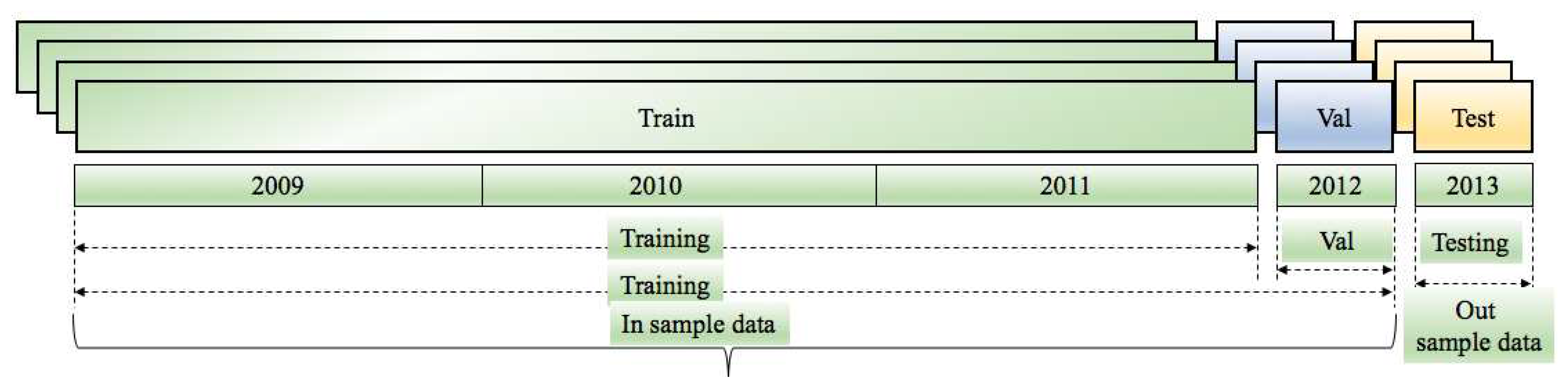
Figure 12.
Breakdown of dataset into training, validation, and testing dataset.
In the case of a FNN, the input is transformed from to . Here, is assumed to consist of k variables, denoted as . Thus, the FNN maps from inputs to one output. In order to account for dummies that have the same value for a given day, we retain only one value per day. Each in the samples should include the demand at time t, the forecasted temperature at time , and dummies for the next day (tomorrow, if t is today). The prediction half-hours would range from to . If we are interested in considering the days after holidays, we should incorporate dummies for the two days following tomorrow. It is important to note that due to holidays falling on weekdays, there are irregularities in the dummies for adjacent days in the dataset. For example, it may follow a pattern such as Monday, Tuesday, Thursday, Friday, Tuesday, and so on. As a result, the dummies are not periodic but rather random in nature.
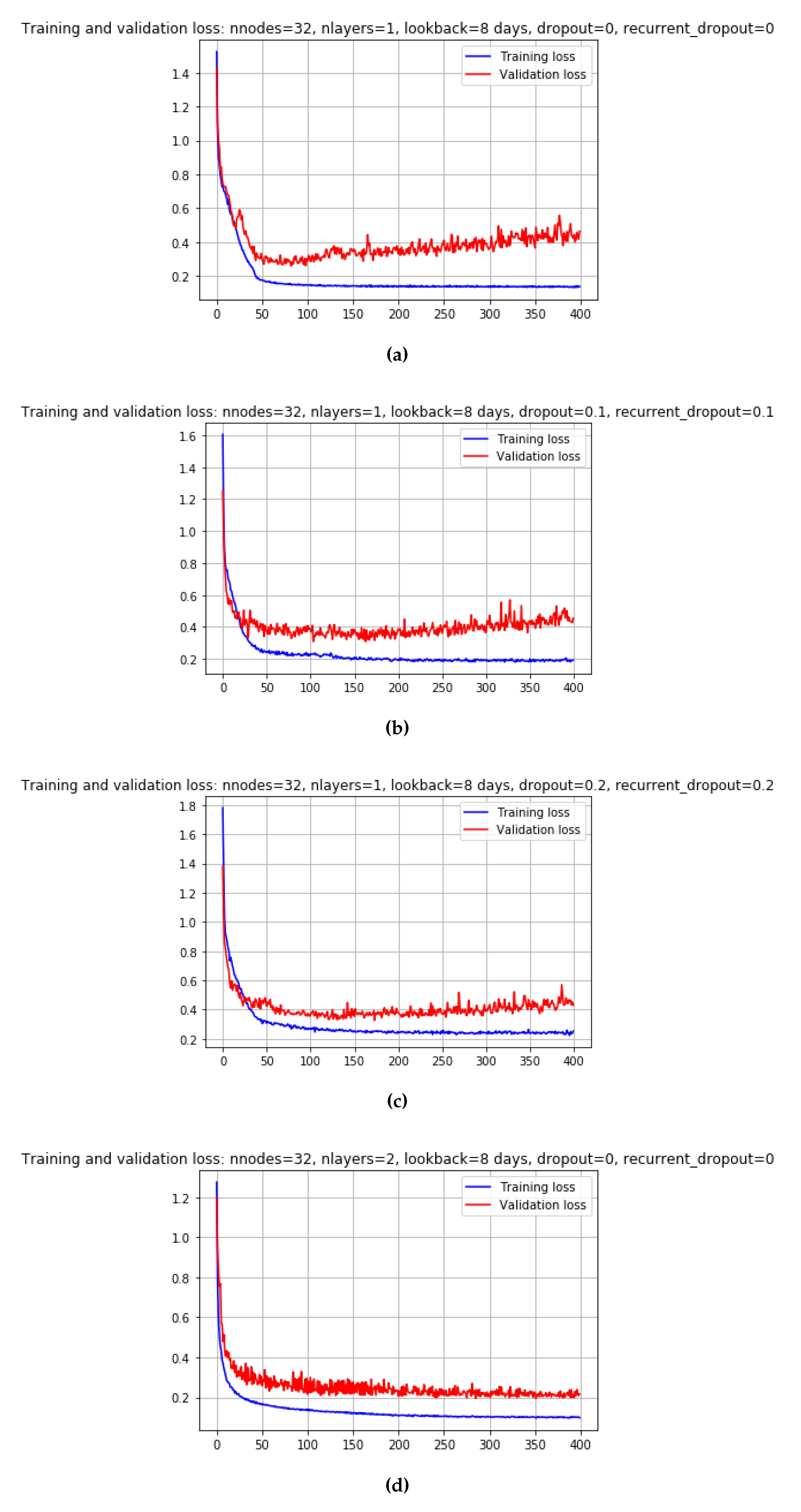
When considering the historical data to predict , particularly when the lookback is large, the LSTM model proves beneficial by avoiding the issue of vanishing or exploding gradients. However, it is important to note that including too much fluctuated information for a large may adversely impact the accuracy of the predictions, as depicted in Figure 13. In the case of holiday data, it may be necessary to have a large , spanning one or multiple years. Conversely, for non-holiday data, the required lookback period is typically on the order of a few days or weeks, with the exception of the days surrounding Songkran and New Year, which may require a lookback period on the order of years. To address this, an approach of treating the interim days together with the holidays () was attempted, but it resulted in poor performance [36].
5.3. Hyper-parameter Tuning
Tuning the hyperparameter shapes the structure of the network and affects the performance of deep networks because they represent the variables as their values are being constantly adjusted to achieve optimal performance of the model [4]. In this experiment, the hyper-parameter optimization process is conducted separately for each deep network. Major hyper-parameters that we considered are,
The process of tuning hyperparameters plays a crucial role in shaping the structure of a network and significantly impacts the performance of deep networks. These hyperparameters represent the variables whose values are continuously adjusted to optimize the model’s performance [4]. In our experiment, we conducted the hyper-parameter optimization process separately for each deep network. The following are the major hyper-parameters:
- 1.
- number of hidden layers,
- 2.
- number of network training iterations,
- 3.
- mini-batch size that denotes the number of time series considered for each full back propagation for each iteration;
- 4.
- epoch that denotes one full forwrd and backward pass through the whole dataset and number of epoch denotes the number of such pass across the dataset are required for optimal training;
- 5.
- Dropout that dropout is a technique to prevent the problem of over-fitting by excluding the negligible influenced neurons from the network. We applied the drop-out for both forward and recurrent.
- 6.
- Look back period that denotes the number of previous timesteps taken to predict the subsequent timestep. In our tuning, we have taken 5 to 10 days lookback period to predict the subsequent timestep of 1 day ahead.
5.4. Critics on ANN
ANNs are highly criticized for their black-box nature and acknowledged in several studies.[1,3,29,36,49]. Unlike multiple regression methods, ANNs are the black-box (lack of interpretability) and they do not offer insights into the correlation of electricity demand and variables. Therefore, Hippert et al. [49] concluded that without a solid understanding of the underlying relationships.
Possibility of overfitting and lack of interpretability are two major drawbacks highlight for ANN domain. Overfitting can occur due to either over-training or over-parameterization. In such overfitted model, training data may well fitted, leading to the poor generalization performance on unnknown test data [1]. Critical comments by Hong et al. [1] mentioned that the good results from ANN is by peeping the properties into the targets. For example, the non-linear autoregressive ANN model was implemented in [11] and achieved 30% improvement on accuracy.
However, due to elastic configuration of ANN structures and non-linearity tackling capability of periodicity, seasonality, and the sequential dependencies of electric demand data sequences, researcher have been applied electricity demand forecasting use cases on ANN and deep learning architecture. In many examples [28,39,41], ANNs already shown outstanding performance on accuracy of electricity demand prediction, nevertheless they do not provide insight into the relationship between electricity demand and its driving factors.
6. Results and discussion
In this section, we empirically determined the hyper-parameters for , , and models for all the four scenarios (, , , and ). However, our prime focus is for the initial two scenarios. The training dataset is a set of data utilized to train the model. During each epoch, the model learns from this data repeatedly, allowing it to grasp the underlying features within the dataset. When the trained model is deployed, it uses this acquired knowledge to make predictions based on the learned patterns.
To ensure the model’s performance and optimize its hyperparameters, a separate validation dataset is created by partitioning it from the training dataset. During the training process, simultaneous validation steps are performed using this validation dataset. The model’s weights are adjusted based on the calculated loss from the validation dataset. One of the main reasons for having a validation dataset is to prevent the model from overfitting the training data, as it provides an independent source for assessing generalization performance.
The test dataset is used to evaluate the model’s performance after it has been trained. This dataset is separate from both the training and validation datasets. In our specific case, the training dataset spans from 2009 to 2011, and the year 2012 is considered as the validation dataset (Figure 12). For testing, the training dataset includes data from 2009 to 2012, while the test dataset consists of data from the year 2013.
6.1. FNN
For the sake of convenience, we have opted for in our analysis, which involves excluding weekends and holidays from the original dataset. Additionally, we have disregarded interim working days like Songkran1D and Newyear1D. In our experiment, we have compiled a list of hyperparameter value sets to be tested specifically for FNN models. These hyperparameter values are presented in Table 4.
The parameters presented in Table 4a were initially implemented to test the functionality and validity of our function. After successfully verifying its performance, some of the parameters were adjusted to observe their impact on the validation results, as shown in Table (Table 4b). was utilized as the metric for measuring performance, and the set of parameters resulting in the minimum validation MAE was selected as the optimal choice. Through our FNN experimental setup, we achieved a minimum validation loss of 162.86 MWatt. This outcome was obtained by selecting a single-layer network with 64 nodes, a look-back period of 5 days, and training the model over 372 epochs. A dropout rate of 0.15 was also applied during the training process to prevent overfitting.
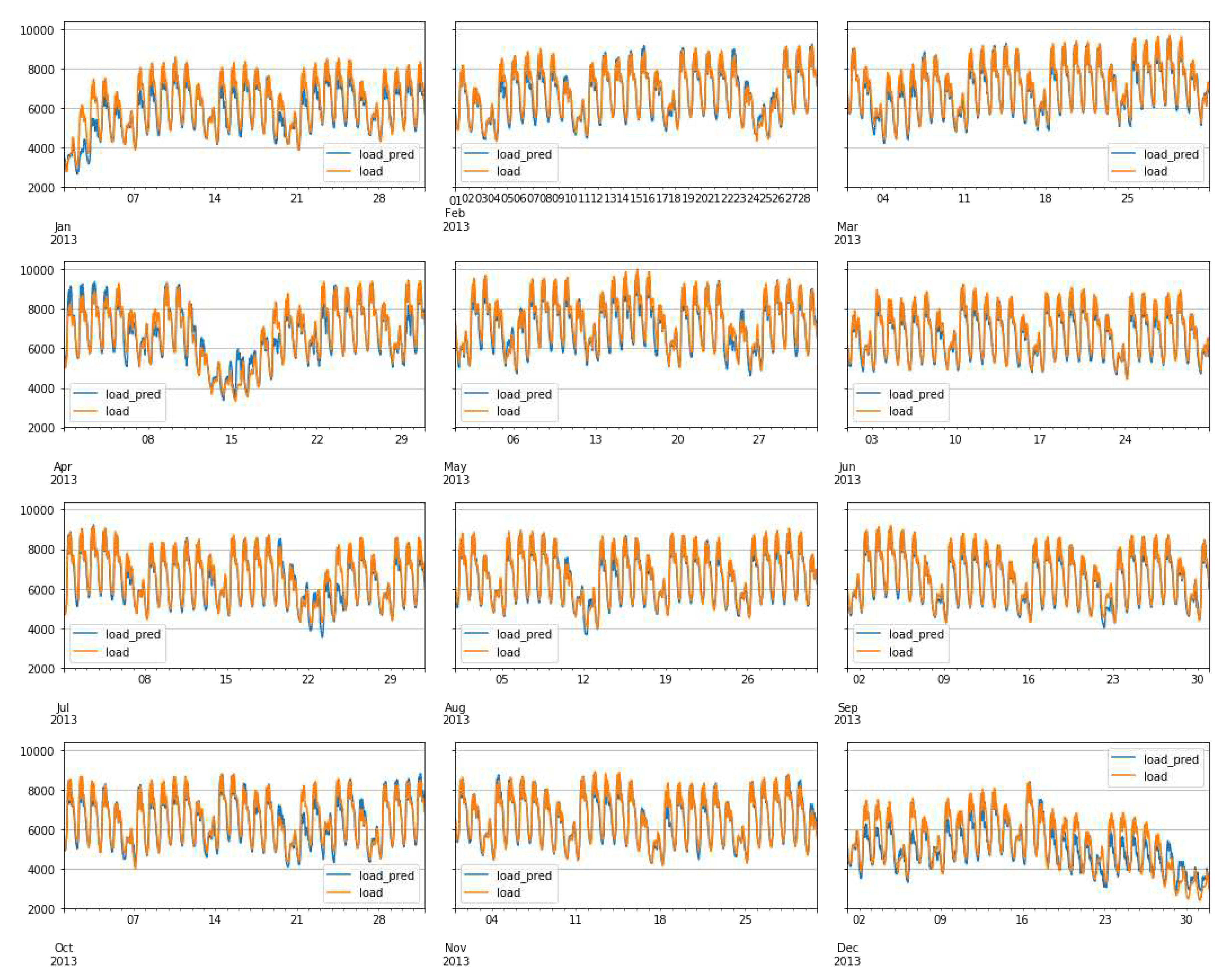
Using the optimized parameters mentioned above, with a dataset size of 44,256 and a test size of 11,520, we conducted predictions for the electricity demand in 2013. The resulting MAPE was found to be 2.47%. It’s important to note that the data setup specifically excluded holidays and weekends, focusing solely on weekdays.The result is presented in Figure 14, where the actual demand is denoted as and forecasting result is denoted as .
6.2. RNN-LSTM
For RNN based LSTM, the look back period is kept fixed for 5 days because we already got the best look back period. Therefore other parameters are varied as,
- Number of nodes =[32, 64]
- Number of layers =[1, 2]
- range of dropout=[0, 0.05, 0.1, 0.15]
- total trainable parameters=66320
The minimum validation loss of 200.75 MWatt is obtained in 51 epochs when 32 nodes of two layer networks is chosen with dropout=0.
By utilizing the optimized parameters mentioned earlier, with a dataset size of 44,256 and a test size of 11,520, we conducted predictions for the electricity demand in 2013. The resulting Mean Absolute Percentage Error (MAPE) was found to be 3.37%. It should be noted that the data setup specifically excluded holidays and weekends, focusing solely on weekdays. The visualization of the prediction results is presented in the accompanying Figure 15, where the actual demand is denoted as and forecasting result is denoted as .
6.3. RNN-GRU
Keeping the fixed look back period as 5 days other hyper-parameters are varied as,
- Number of nodes=[32, 64]
- Number of layers=[1, 2]
- Range of dropout=[0, 0.05, 0.1, 0.15]
- Total trainable parameters=66320
This RNN based GRU experimental setup which gives the minimum validation loss of 195.31 MWatt is obtained in 69 epochs when 32 nodes of single layer network is chosen with dropout=0.
Using the optimized parameters mentioned above, with a dataset size of 44,256 and a test size of 11,520, we conducted predictions for the electricity demand in 2013. The resulting MAPE was found to be 2.58%. It should be noted that the data setup specifically excluded holidays and weekends, focusing solely on weekdays. The visualization of the prediction results can be seen in Figure 16, where the actual demand is represented as and the forecasting results are denoted as .
As the parameters for the GRU and LSTM models are still not fully optimized, the corresponding test MAPEs are as follows,

Table 5.
MAPE comparison for working days.
| Methods | MAPE | MAE |
| FNN | 2.47 | 163.9 |
| GRU | 2.58 | 169.5 |
| LSTM | 3.37 | 228.18 |
| Naive | 4.93 | 312.34 |
According to Table A2, the minimum loss of 170.41 MW is achieved when the parameters are set as follows: nnodes = 32, nlayers = 2, look back = 10 days, and dropout = 0, over the course of 351 epochs. These optimized parameters were implemented, along with some trial and error values, to assess the inclusion of certain variables and determine their impact on the model’s performance.
For instance, excluding the month variable did not lead to a significant improvement in MAPE when using the FNN model. However, incorporating the maximum temperature variable resulted in an improvement of 1.39 MW in MAE and a MAPE of 2.54% (Figure 17). This indicates that including the maximum temperature variable enhanced the model’s predictive accuracy
Considering the entire dataset, which includes demand values for holidays, weekends, and weekdays, we can set the lookback period to 8 days. By varying the parameters and optimizing the models, we achieved the following results,
- •
- For the FNN model, the minimum validation loss of 213.98 MW was obtained when nnodes=64, nlayers=2, lookback=8 days, dropout=0, and epoch=161.
- •
- For the GRU model, the minimum validation loss of 243.72 MW occurred when nnodes=64, nlayers=2, lookback=8 days, dropout=0, and epoch=56.
- •
- Similarly, for the LSTM model, the minimum validation loss of 234.22 MW was achieved when nnodes=64, nlayers=2, lookback=8 days, dropout=0, and epoch=99.
Based on above tables, the best parameters are picked up and implemented for a day ahead prediction. The overall results are summarized as,
Table 6.
Implementation of best parameters: Day ahead forecast.
| Model | nnodes/layer | nlayers | dropout | epoch | Min MAE | Test MAE | Test MAPE(%) |
| FNN | 64 | 2 | 0 | 161 | 214.0 | 212.8 | 3.15 |
| GRU | 64 | 2 | 0 | 56 | 243.7 | 210.3 | 2.44 |
| LSTM | 64 | 2 | 0 | 200 | 252.2 | 246.2 | 3.86 |
| Naive | - | - | - | - | - | 669.0 | - |
Since the performance is analyzed from the validation result, FNN shows the best MAE MW. Nevertheless, test performances (both MAE and MAPE) are better in model.
When the prediction was made on the FNN, LSTM, and GRU networks trained by using the aggregate data and testing for 2013, obtained result is tabulated as in Table 7.
Figure 18.
Prediction for 2013 using whole data set altogether for FFNN
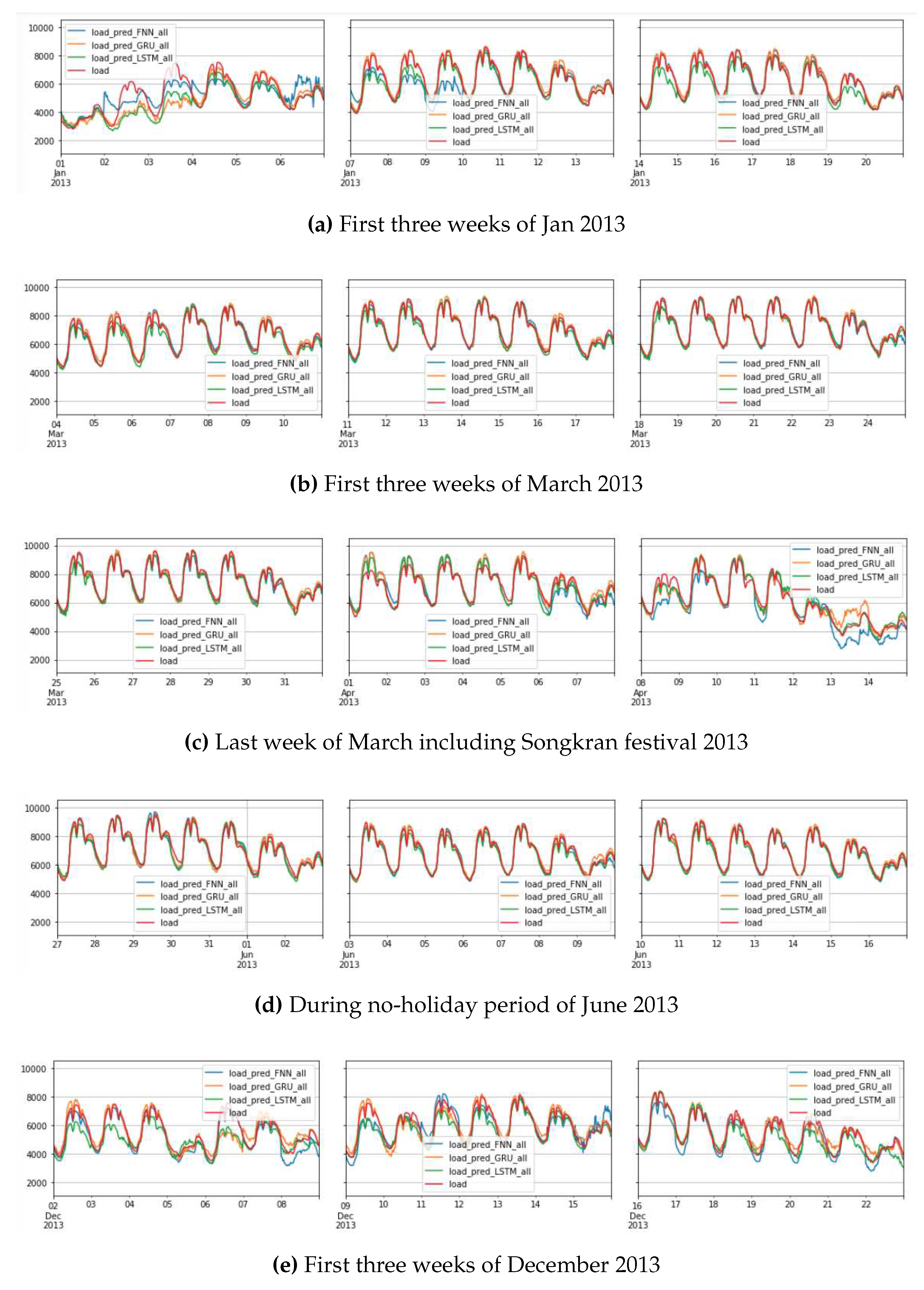
When our analysis was limited to non-holiday weekdays, there was no need to include holiday-type dummies or interim dummies in the modeling process. However, when dealing with holidays, it becomes necessary to incorporate holiday-type dummies because different holidays can have varying effects on electricity demand. For example, holidays like Songkran tend to significantly reduce the load. It’s worth noting that networks with larger variables, such as capacity, generally pose more challenges in terms of training, making it more difficult to achieve the minimum loss.
Figure 19.
Prediction of demand: using FFNN, GRU, & LSTM for whole data set altogether for 2013
7. Conclusion
This paper introduces a novel approach for STLF by constructing four different scenarios to train the models using appropriate datasets. The selection of optimal parameters from the hyperparameters was conducted through experiments. The results demonstrate that deep networks are highly influenced by the number of hidden layers and neurons per layer. In the case of , the model exhibited superior accuracy. Similarly, by fine-tuning the hyperparameters, the best parameters were determined for the other models, such as and . These obtained parameters were then applied to all three models for day-ahead forecasting of electricity demand in the year 2013.
A comparative study was conducted to evaluate the forecasting accuracy across different scenarios. When forecasting for non-holiday periods using the dataset from , the FNN model achieved the lowest MAPE of 2.47%. In contrast, when predicting the same testing dataset (non-holidays) using the dataset from , the model achieved a slightly higher MAPE of 2.71%, approximately 10% higher. As the dataset for specifically consists of non-holiday weekdays, it is evident that provides better accuracy compared to the dataset from .
Based on these findings, we can implement STLF by categorizing the dataset into two distinct scenarios. can be utilized to predict electricity demand for working days (Monday to Friday), while can be employed to forecast demand for weekends (Saturday and Sunday) and holidays with improved accuracy.
Acknowledgments
We would like to express our sincere appreciation to Assoc. Prof. Chawalit Jeenanunta, and the EGAT for providing the necessary dataset used in this research.
Appendix. Tuning of Hyper-parameter
Hyper-parameter selection for , is described in the Table A1, where FNN method outperforms rest of other methods. Now the variation over following parameters are performed for the outperformed FNN method to find out the best parameters value.
Table A1.
Variation of parameters and corresponding results
| Parameters | FNN Results | GRU Results | LSTM Results | ||||||
|---|---|---|---|---|---|---|---|---|---|
| nnodes | nlayers | look back | dropout | MAE | epochs | MAE | epochs | MAE | epochs |
| 32 | 1 | 5 | 0 | 226.09 | 319 | 195.31 | 69 | 234.16 | 39 |
| 32 | 1 | 5 | 0.05 | 179.33 | 362 | 204.72 | 72 | 251.48 | 30 |
| 32 | 1 | 5 | 0.1 | 184.27 | 384 | 217.90 | 50 | 223.01 | 50 |
| 32 | 1 | 5 | 0.15 | 205.24 | 327 | 228.40 | 80 | 223.52 | 81 |
| 32 | 1 | 10 | 0 | 264.73 | 196 | NA | NA | NA | NA |
| 32 | 1 | 10 | 0.05 | 231.74 | 302 | NA | NA | NA | NA |
| 32 | 1 | 10 | 0.1 | 196.73 | 399 | NA | NA | NA | NA |
| 32 | 1 | 10 | 0.15 | 197.42 | 348 | NA | NA | NA | NA |
| 32 | 2 | 5 | 0 | 271.67 | 377 | 226.19 | 72 | 200.75 | 51 |
| 32 | 2 | 5 | 0.05 | 259.13 | 136 | 213.24 | 79 | 240.31 | 89 |
| 32 | 2 | 5 | 0.1 | 272.13 | 89 | 235.56 | 57 | 225.07 | 64 |
| 32 | 2 | 5 | 0.15 | 238.8 | 62 | 233.29 | 71 | 224.44 | 100 |
| 32 | 2 | 10 | 0 | 170.41 | 351 | NA | NA | NA | NA |
| 32 | 2 | 10 | 0.05 | 185.37 | 395 | NA | NA | NA | NA |
| 32 | 2 | 10 | 0.1 | 189.83 | 260 | NA | NA | NA | NA |
| 32 | 2 | 10 | 0.15 | 200.49 | 328 | NA | NA | NA | NA |
| 64 | 1 | 5 | 0 | 230.31 | 153 | 221.11 | 79 | 241.49 | 88 |
| 64 | 1 | 5 | 0.05 | 189.14 | 322 | 205.10 | 72 | 214.19 | 40 |
| 64 | 1 | 5 | 0.1 | 255.40 | 307 | 222.80 | 66 | 253.20 | 51 |
| 64 | 1 | 5 | 0.15 | 245.71 | 53 | 207.48 | 78 | 251.50 | 63 |
| 64 | 1 | 10 | 0 | 193.33 | 391 | NA | NA | NA | NA |
| 64 | 1 | 10 | 0.05 | 198.98 | 142 | NA | NA | NA | NA |
| 64 | 1 | 10 | 0.1 | 210.31 | 351 | NA | NA | NA | NA |
| 64 | 1 | 10 | 0.15 | 191.81 | 399 | NA | NA | NA | NA |
| 64 | 2 | 5 | 0 | 314.57 | 140 | 207.66 | 67 | 219.21 | 100 |
| 64 | 2 | 5 | 0.05 | 314.30 | 141 | 227.20 | 61 | 212.24 | 99 |
| 64 | 2 | 5 | 0.1 | 278.63 | 386 | 240.29 | 71 | 218.14 | 67 |
| 64 | 2 | 5 | 0.15 | 293.13 | 126 | 236.68 | 78 | 227.72 | 77 |
| 64 | 2 | 10 | 0 | 220.30 | 356 | NA | NA | NA | NA |
| 64 | 2 | 10 | 0.05 | 192.39 | 340 | NA | NA | NA | NA |
| 64 | 2 | 10 | 0.1 | 218.01 | 365 | NA | NA | NA | NA |
| 64 | 2 | 10 | 0.15 | 216.56 | 349 | NA | NA | NA | NA |
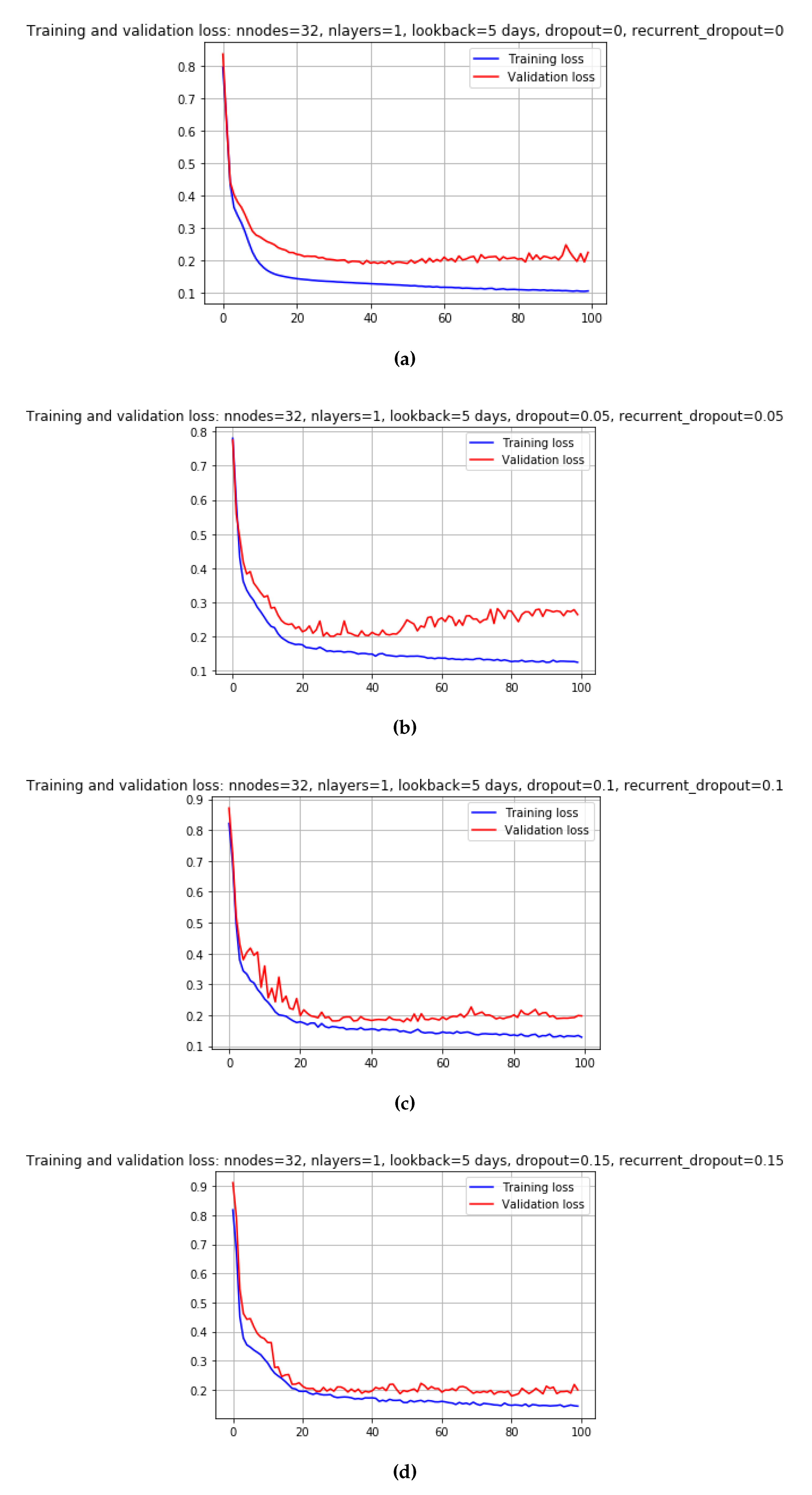
Figure A1.
Few graphs for hyper-parameter testing for Scenario1
Hyper-parameter selection for ,
Table A2.
Variation of parameters and corresponding results
| Parameters | FNN Results | GRU Results | LSTM Results | |||||
|---|---|---|---|---|---|---|---|---|
| nnodes | nlayers | dropout | MAE | epoch | MAE | epoch | MAE | epoch |
| 32 | 1 | 0 | 323.95 | 83 | 269.42 | 71 | 265.85 | 57 |
| 32 | 1 | 0.1 | 387.77 | 164 | 251.01 | 41 | 276.99 | 34 |
| 32 | 1 | 0.2 | 409.22 | 174 | 281.80 | 76 | 267.53 | 55 |
| 32 | 2 | 0 | 243.30 | 352 | 251.17 | 53 | 305.92 | 97 |
| 32 | 2 | 0.1 | 266.86 | 304 | 278.23 | 67 | 274.52 | 97 |
| 32 | 2 | 0.2 | 276.40 | 349 | 280.47 | 99 | 265.23 | 52 |
| 32 | 3 | 0 | 227.40 | 96 | 284.14 | 97 | 306.19 | 58 |
| 32 | 3 | 0.1 | 232.65 | 374 | 293.56 | 98 | 281.66 | 38 |
| 32 | 3 | 0.2 | 273.96 | 209 | 274.05 | 73 | 275.03 | 99 |
| 64 | 1 | 0 | 339.85 | 59 | 263.20 | 82 | 284.72 | 68 |
| 64 | 1 | 0.1 | 327.44 | 51 | 275.22 | 99 | 319.13 | 19 |
| 64 | 1 | 0.2 | 388.25 | 68 | 290.82 | 97 | 269.69 | 43 |
| 64 | 2 | 0 | 224.12 | 324 | 243.72 | 56 | 234.22 | 99 |
| 64 | 2 | 0.1 | 277.33 | 289 | 281.96 | 77 | 254.63 | 97 |
| 64 | 2 | 0.2 | 311.62 | 369 | 296.06 | 80 | 279.30 | 92 |
| 64 | 3 | 0 | 237.82 | 180 | 266.50 | 95 | 296.79 | 88 |
| 64 | 3 | 0.1 | 279.02 | 288 | 286.08 | 92 | 281.90 | 87 |
| 64 | 3 | 0.2 | 296.57 | 66 | 290.56 | 93 | 260.95 | 100 |
Figure A2.
Few graphs for hyper-parameter testing for Scenario2
Now for GRU, the min val loss of 243.72 happens when nnodes=64, nlayers=2, lookback=8 days, dropout=0 and epoch=56.0. Similarly for LSTM, The min val loss of 234.22 happens when nnodes=64, nlayers=2, lookback=8 days, dropout=0 and epoch=99.0.
References
- Hong, T.; Shu, F. Probabilistic electric load forecasting: A tutorial review. Int. J of Forecasting 2016, 3, 32–914. [Google Scholar] [CrossRef]
- Raza, M.; Khosravi, A. A review on artificial intelligence based load demand forecasting techniques for smart grid and buildings. Renewable and Sustainable Energy Reviews 2015, 50, 1352–1372. [Google Scholar] [CrossRef]
- Makridakis, S.; Spiliotis, E.; Assimakopoulus, V. Statistical and machine learning fore- casting methods: Concerns and ways forward. Plos One 2018, 13, 3–e0194889. [Google Scholar] [CrossRef]
- Stosov, M.A.; Radivojevic, N.; Ivanova, M. Electricity Consumption Prediction in an Electronic System Using Artificial Neural Networks. Electronics, mdpi 2022, 11, 3506. [Google Scholar] [CrossRef]
- Roman-Portabales, A.; Lopez-Nores, M.; Pazos-Arias, J.J. Systematic Review of Electricity Demand Forecast Using ANN-Based Machine Learning Algorithms. Sensors, mdpi 2021, 21, 4544. [Google Scholar] [CrossRef]
- McCulloch, J.; Ignatieva, K. Forecasting High Frequency Intra-Day Electricity Demand Using Temperature. SSRN Electr. J. 2017. [Google Scholar] [CrossRef]
- Hewamalage, H.; Christoph, B.; Kasum, B. Recurrent Neural Networks for Time Series Forecasting: Current Status and Future Directions. Int. J. of Forecasting 2019, 17, 388–427. [Google Scholar] [CrossRef]
- Chapagain, K.; Kittipiyakul, S. Performance Analysis of Short-Term Electricity Demand with Atmospheric Variables. Energies 2018, 11. [Google Scholar] [CrossRef]
- Clements, A.E.; Hurn, A.S.; Li, Z. Forecasting day-ahead electricity load using a multiple equation time series approach. Eur. J. Oper. Res. 2016, 251, 522–530. [Google Scholar] [CrossRef]
- Lusis, P.; Khalilpour, K.; Andrew, L.; Liebman, A. Short-term residential load forecasting: Impact of calendar effects and forecast granularity. Appl. Energy 2017, 205, 654–669. [Google Scholar] [CrossRef]
- Buitrago, J.; Asfour, S. Short-Term Forecasting of Electric Loads Using Nonlinear Autoregressive Artificial Neural Networks with Exogenous Vector Inputs. Energies 2017, 10, 40. [Google Scholar] [CrossRef]
- Taylor, J.W.; de Menezes, L.M.; McSharry, P.E. A comparison of univariate methods for forecasting electricity demand up to a day ahead. Int. J. Forecast. 2006, 22, 1–16. [Google Scholar] [CrossRef]
- Hong, T.; Wang, P.; Willis, H.L. Short Term Electric Load Forecasting. Int. J. Forecast. 2010, 74, 1–6. [Google Scholar] [CrossRef]
- Hong, T.; Wang, P. Fuzzy interaction regression for short term load forecasting. Fuzzy Opt. Decis. Mak. 2014, 13, 91–103. [Google Scholar] [CrossRef]
- Dang-Ha, H.; Filippo, M.B.; Roland, O. Local Short Term Electricity Load Forecasting: Automatic Approaches. arXiv 2017. Available online: https://arxiv.org/pdf/1702.08025.pdf.
- Selvi, M.; Mishra, S. Investigation of Weather Influence in Day-Ahead Hourly Electric Load Power Forecasting with New Architecture Realized in Multivariate Linear Regression & Artificial Neural Network Techniques. 8th IEEE India International Conference on Power Electronics (IICPE) 2018, 13-15. [Google Scholar]
- Ramanathan, R.; Engle, R.; Granger, C.W.; Vahid-Araghi, F.; Brace, C. Short-run forecasts of electricity loads and peaks. Int. J. Forecast. 1997, 13, 161–174. [Google Scholar] [CrossRef]
- Chapagain, K.; Sato, T.; Kittipiyakul, S. Performance analysis of short-term electricity demand with meteorological parameters. In Proceedings of the 2017 14th Int Conf on Electl Eng/Elx, Computer, Telecom and IT (ECTI-CON), Phuket, Thailand, 27–30 June 2017; pp. 330–333. [Google Scholar]
- Ismail, Z.; Jamaluddin, F.; Jamaludin, F. Time Series Regression Model for Forecasting Malaysian Electricity Load Demand. Asian J. Math. Stat. 2008, 1, 139–149. [Google Scholar] [CrossRef]
- Bouktif, S.; Fiaz, A.; Ouni, A.; Serhani, M. Multi-Sequence LSTM-RNN Deep Learning and Metaheuristics for Electric Load Forecasting. Energies 2020, 13, 391. [Google Scholar] [CrossRef]
- Bouktif, S.; Fiaz, A.; Ouni, A.; Serhani, M. Optimal Deep Learning LSTM Model for Electric Load Forecasting using Feature Selection and Genetic Algorithm: Comparison with Machine Learning Approaches. Energies 2018, 7, 1636. [Google Scholar] [CrossRef]
- Torabi, M.; Hashemi, S. A data mining paradigm to forecast weather sensitive short-term energy consumption. 16th CSI International Symposium on Artificial Intelligence and Signal Processing (AISP 2012) 2012. [Google Scholar]
- Pramono, S.H.; Rohmatillah, M.; Maulana, E.; Hasanah, R.N.; Hario, F. Deep learning-based short-term load forecasting for supporting demand response program in hybrid energy system. Energies 2019, 12, 17. [Google Scholar] [CrossRef]
- Kim, T.Y.; Cho, S.B. Predicting residential energy consumption using CNN-LSTM neural networks. Energy 2019, 182, 72–81. [Google Scholar] [CrossRef]
- Qi, Z.; Zheng, X.; Chen, Q. A short term load forecasting of integrated energy system based on CNN-LSTM. Web of Conferences 2020, E3S. [Google Scholar] [CrossRef]
- Gourav, K.; Uday, P.S.; Sanjeev, Jain. An adaptive particle swarm optimization-based hybrid long short-term memory model for stock price time series forecasting. Soft Computing, Springer 2022, 26, 12115–12135. [Google Scholar] [CrossRef]
- Hong, T.; Xiangzheng, L.; Liangzhi, L.; Lian, Z.; Yu, Y.; Xiaohui, H. One-shot pruning of gated recurrent unit neural network by sensitivity for time-series prediction. Neurocomputing, Elsevier 2022, 512, 15–24. [Google Scholar] [CrossRef]
- Machado, E.; Pinto, T.; Guedes, V.; Morais, H. Demand Forecasting Using Feed-Forward Neural Networks. Energies 2021, 14, 7644. [Google Scholar] [CrossRef]
- Shereen, E.; Daniela, T.; Ahmed, R.; Hadi, S.J.; Lars, S.T. Do We Really Need Deep Learning Models for Time Series Forecasting. Computer Science, arXiv 2021. [Google Scholar] [CrossRef]
- Parkpoom, S.; Harrison, G.P. Analyzing the Impact of Climate Change on Future Electricity Demand in Thailand. IEEE Trans. Power Syst. 2008, 23, 1441–1448. [Google Scholar] [CrossRef]
- Chapagain, K.; Kittipiyakul, S. Short-Term Electricity Demand Forecasting with Seasonal and Interactions of Variables for Thailand. In Proceedings of the 2018 Int Electrl Eng Congress (iEECON), Krabi, Thailand, 7–9 March 2018; pp. 1–4. [Google Scholar] [CrossRef]
- Chapagain, K.; Kittipiyakul, S. Short-term Electricity Load Forecasting Model and Bayesian Estimation for Thailand Data. In Proceedings of the 2016 Asia Conf on Power and Electl Engg (ACPEE 2016), Bankok, Thailand, 20–22 March 2016; Volume 55, p. 06003. [Google Scholar]
- Phyo, P.; Jeenanunta, C. Electricity Load Forecasting using a Deep Neural Network. Eng. Appl. Sci. Res. 2019, 46, 10–17. [Google Scholar]
- Su, W.H.; Jeenanunta, C. Short-term Electricity Load Forecasting in Thailand: An Analysis on Different Input Variables. In IOP Conference Series: Earth and Environmental Science; IOP Publishing: Bristol, UK, 2018. [Google Scholar] [CrossRef]
- Darshana, A.K.; Chawalit, J. Hybrid Particle Swarm Optimization with Genetic Algorithm to Train Artificial Neural Networks for Short-term Load Forecasting. Int. J. Swarm Intell. Res. 2019, 10, 1–14. [Google Scholar]
- Chapagain, K.; Kittipiyakul, S.; Kulthanavit, P. Short-Term Electricity Demand Forecasting: Impact Analysis of Temperature for Thailand. Energies 2020, 13, 2498. [Google Scholar] [CrossRef]
- Sankalpa, C.; Kittipiyakul, S.; Laitrakun, S. Short-Term Electricity Load Using Validated Ensemble Learning. Energies 2022, 15, 2498. [Google Scholar] [CrossRef]
- Harun, M.H.H.; Othman, M.M.; Musirin, I. Short term Load Forecasting using Artificial Neural Network based Multiple lags and Stationary Timeseries. 2010 4th International Power Engineering and Optimization Conference (PEOCO) 2010, 363-370. [Google Scholar]
- Tee, C.Y; Cardell, J.B.; Ellis, G.W. Short term Load Forecasting using Artificial Neural Network. 41st North American Power Symposium 2009, 1–6. [Google Scholar]
- Li, B.; Lu, M.; Zhang, Y.; Huang, J. A Weekend Load Forecasting Model Based on Semi-Parametric Regression Analysis Considering Weather and Load Interaction. Energies 2019, 12, 1–19. [Google Scholar] [CrossRef]
- Cao, Z.; Han, X.; Lyons, W.; Fergal, O. Energy management optimisation using a combined Long Short term Memory recurrent neural network-Particle Swarm Optimization model. J of Clear Production, Elsevier 2022, 326. [Google Scholar]
- Li, Y.; Pizer, W.A.; Wu, L. Climate change and residential electricity consumption in the Yangtze River Delta, China. Proc. Natl. Acad. Sci. USA 2019, 116, 472–477. [Google Scholar] [CrossRef]
- Apadula, F.; Bassini, A.; Elli, A.; Scapin, S. Relationships between meteorological variables and monthly electricity demand. Appl. Energy 2012, 98, 346–356. [Google Scholar] [CrossRef]
- Sailor, D.; Pavlova, A. Air conditioning market saturation and long-term response of residential cooling energy demand to climate change. Energy 2003, 28, 941–951. [Google Scholar] [CrossRef]
- Chapagain, K.; Kittipiyakul, S. Short-term Electricity Load Forecasting for Thailand. In Proceedings of the 2018 15th International Conference on Electrical Engineering/Electronics, Computer, Telecommunications and Information Technology (ECTI-CON), Chiang Rai, Thailand, 18–21 July 2018; pp. 521–524. [Google Scholar] [CrossRef]
- Darshana, A.K.; Chawalit, J. Combine Particle Swarm Optimization with Artificial Neural Networks for Short-Term Load Forecasting. Int. Sci. J. Eng. Technol 2017, 1, 25–30. [Google Scholar]
- Cottet, R.; Smith, M. Bayesian Modeling and Forecasting of Intraday Electricity Load. J. Am. Stat. Assoc. 2003, 98, 839–849. [Google Scholar] [CrossRef]
- Dilhani, M.H.M.R.S.; Jeenanunta, C. Daily electric load forecasting: Case of Thailand. In Proceedings of the 2016 7th Int Conf of Inf and Comm Tech for Embedded Sys (IC-ICTES), Bangkok, Thailand, 20–22 March 2016; pp. 25–29. [Google Scholar] [CrossRef]
- Hippert, H.S.; Pedreira, C.E.; Souza, R.C. Neural networks for short-term load forecasting: a review and evaluation. IEEE Trans. Power Syst. 2001, 16, 44–55. [Google Scholar] [CrossRef]
- Shi, H.; Xu, M.; Li, R. Deep Learning for Household Load Forecasting Novel Pooling Deep RNN. IEEE Trans. Smart Grid 2018, 9, 5271–5280. [Google Scholar] [CrossRef]
- Soares, L.J.; Souza, L.R. Forecasting electricity demand using generalized long memory. Int. J. Forecast. 2006, 22, 17–28. [Google Scholar] [CrossRef]
- Wang, Y.; Niu, D.; Ji, L. Short-term power load forecasting based on IVL-BP neural network technology. Syst. Eng. Procedia 2012, 4, 168–174. [Google Scholar] [CrossRef]
- Bandara, K.; Bergmeir, C.; Smyl, S. Forecasting across time series databases using recurrent neural networks on groups of similar series: A clustering approach. Expert Systems with Applications. Expert System with Applications 2019, 140, 112896. [Google Scholar] [CrossRef]
- Alya, A.; Ameena, S.A.; Mousa, M.; Rajesh, K.; Ahmed, A.Z.D. Short-term load and price forecasting using artificial neural network with enhanced Markov chain for ISO New England. Energy Reports, Elsevier 2023, 4799-4815. [Google Scholar] [CrossRef]
- Hongli, L.; Luoqi, W.; Ji, L.; Lei, S. Research on Smart Power Sales Strategy Considering Load Forecasting and Optimal Allocation of Energy Storage System in China. Energies, mdpi 2023, 16, 3341. [Google Scholar] [CrossRef]
- Kittiwoot, C.; Vorapat, I.; Anothai, T. Electricity Consumption in Higher Education Buildings in Thailand during the COVID-19 Pandemic. Buildings, mdpi 2022, 12, 1532. [Google Scholar] [CrossRef]
Figure 1.
Architecture of a Feedforward Neural Networks [28].
Figure 1.
Architecture of a Feedforward Neural Networks [28].
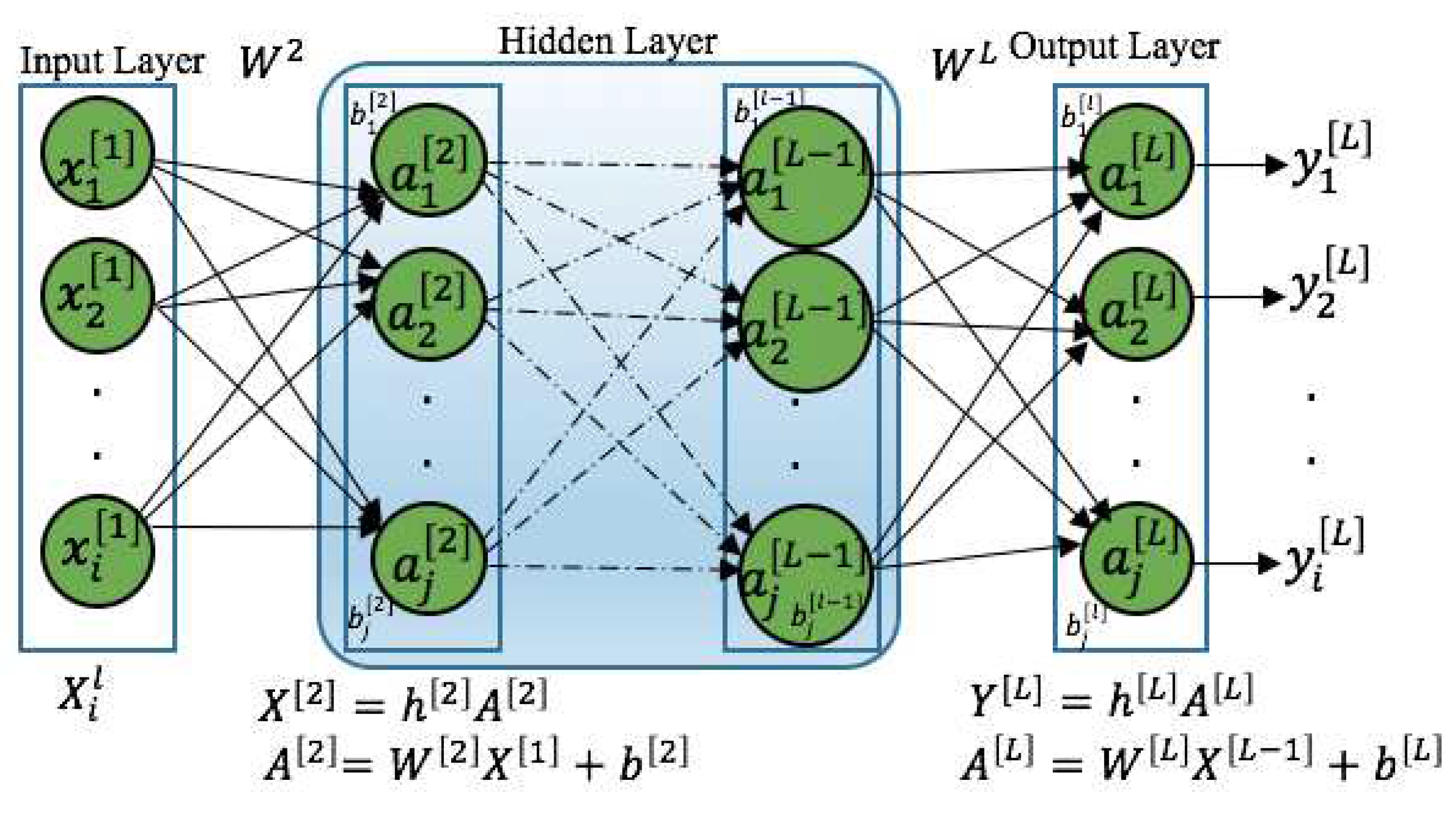
Figure 2.
Architecture of LSTM [26].
Figure 2.
Architecture of LSTM [26].
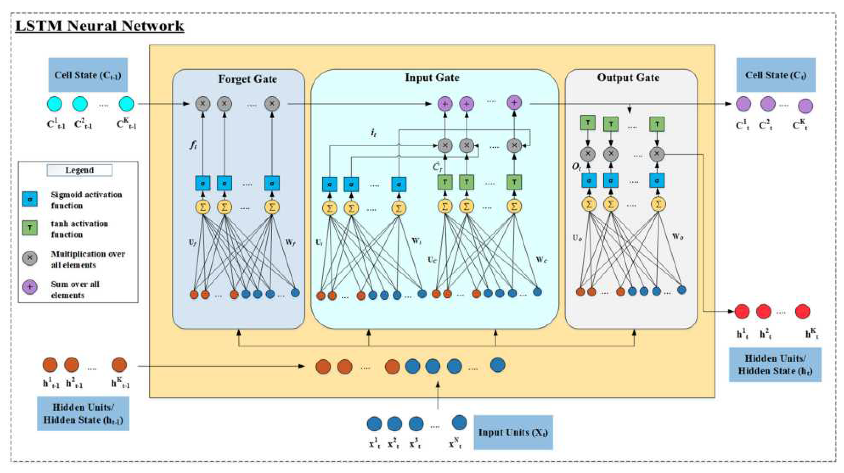
Figure 3.
Architecture of GRU: flow of information [27].
Figure 3.
Architecture of GRU: flow of information [27].
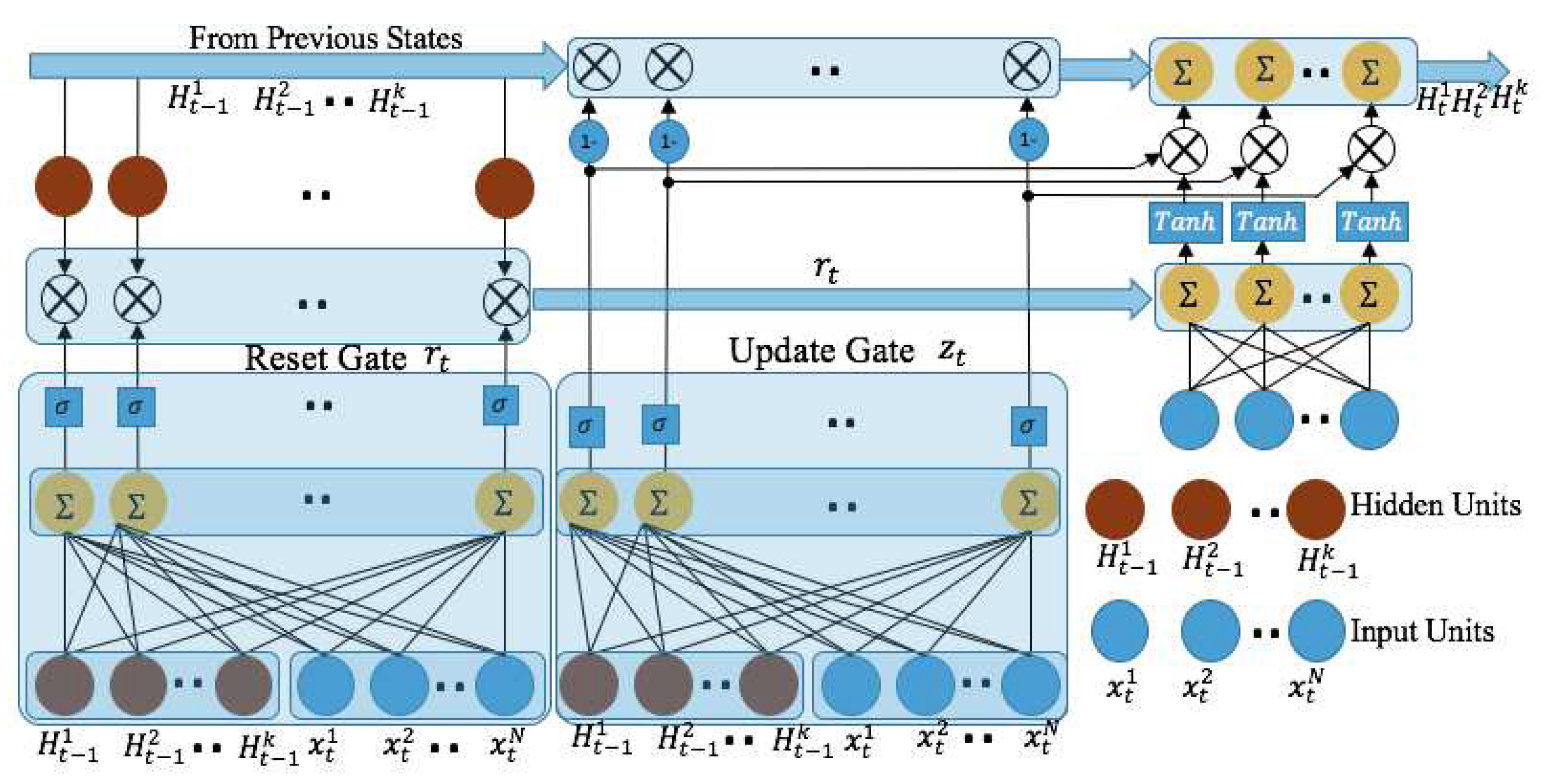
Figure 4.
(a) Complete demand profile for a year: 2012 (b) Overall demand profile with trend.
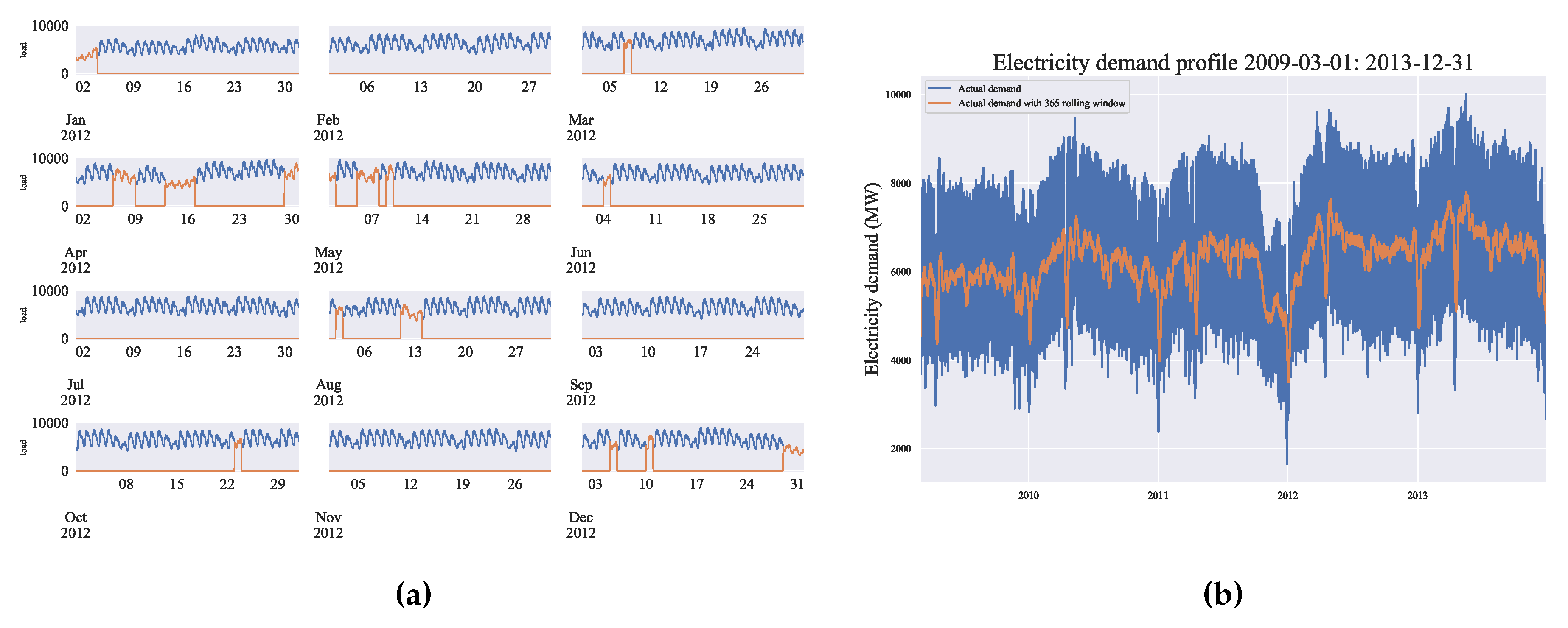
Figure 5.
(a) Decrease of load during Bangkok-flood (b) Day type (calendar) variation on load.
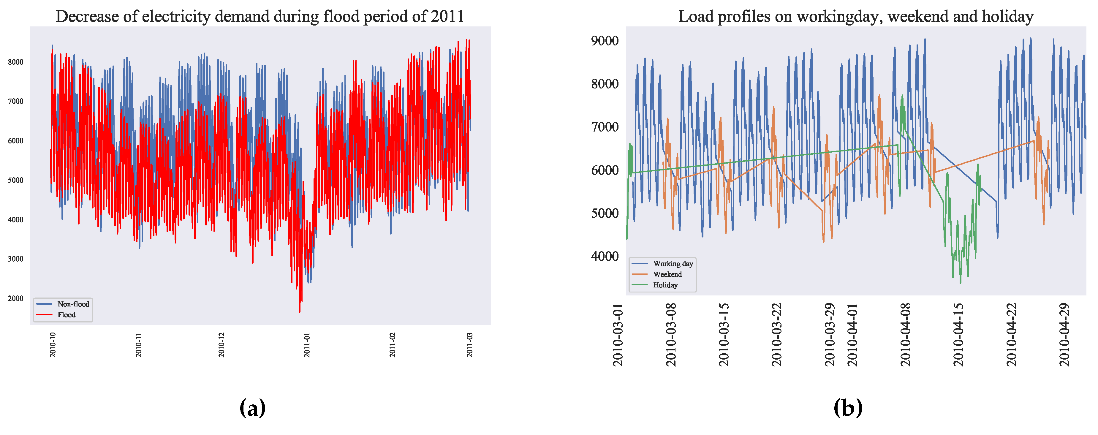
Figure 6.
(a) Electricity demand during Songkran period (b) Decrease of electricity demand during New Year period.
Figure 6.
(a) Electricity demand during Songkran period (b) Decrease of electricity demand during New Year period.
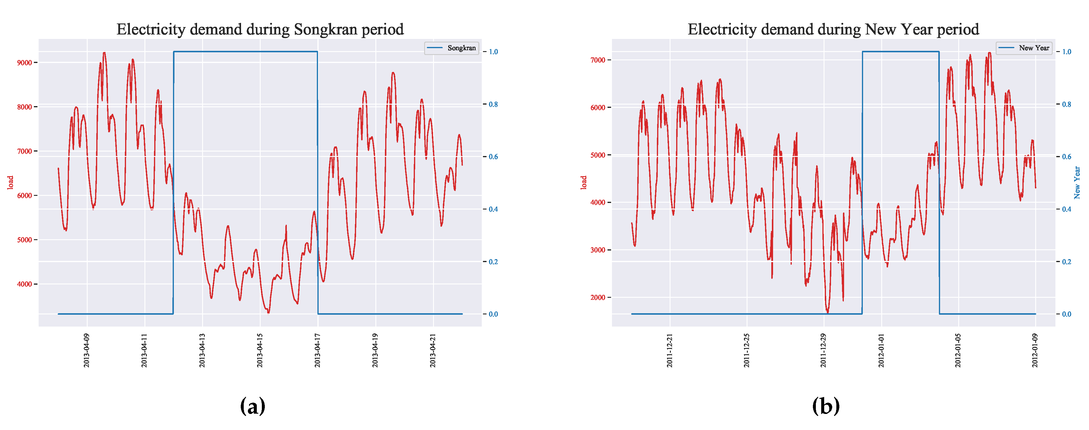
Figure 7.
Variation of demand over a year and months.
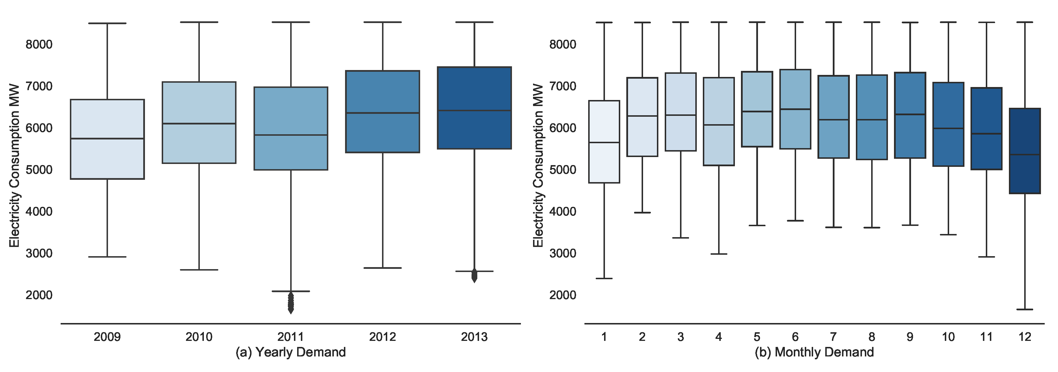
Figure 8.
(a) Effect of temperature during peak hour (b) Effect of temperature at two different hours [36].
Figure 8.
(a) Effect of temperature during peak hour (b) Effect of temperature at two different hours [36].
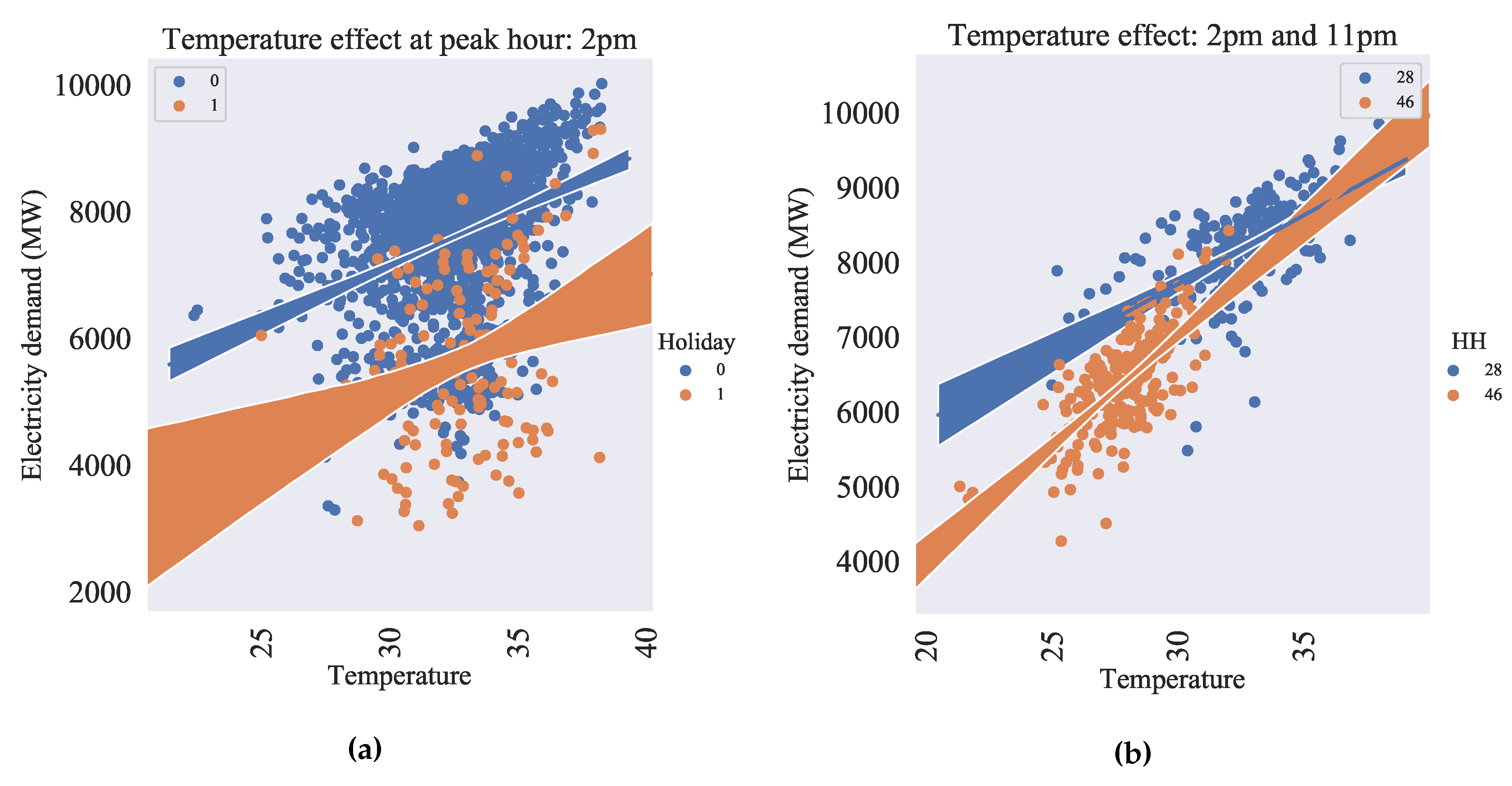
Figure 9.
Proposed forecasting methodology.
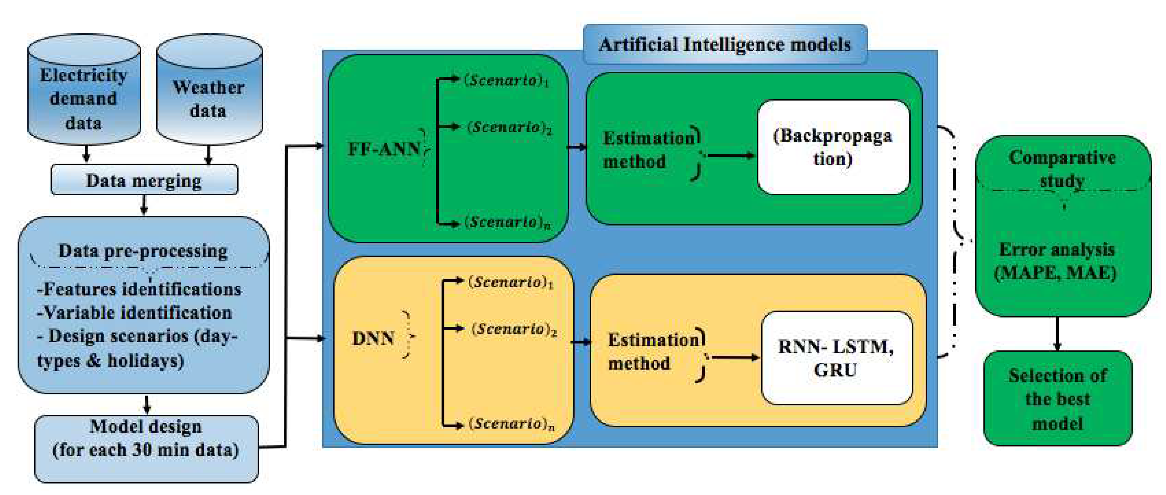
Figure 10.
(a) Data input structure on FNN model. (b) Data input structure on DNN.
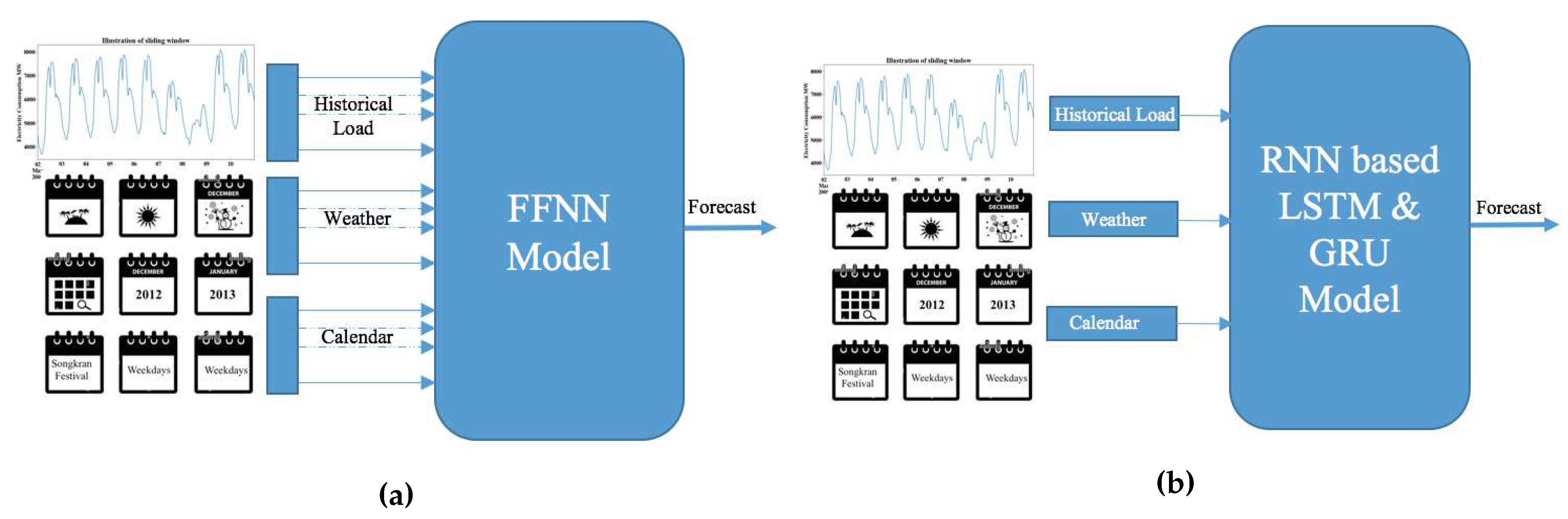
Figure 11.
Demand prediction horizon: practice of EGAT, Thailand.
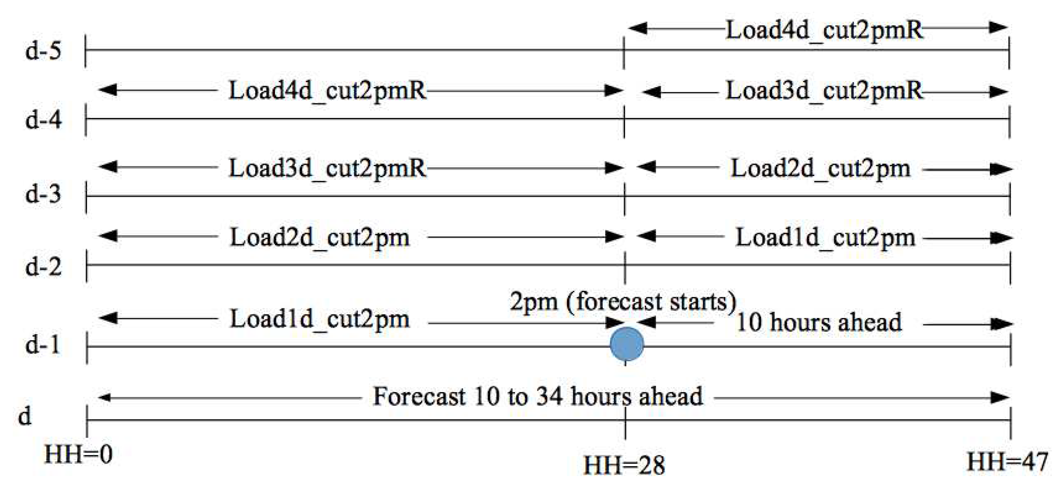
Figure 13.
Visualization of pre-trained model, look-back period, and prediction.
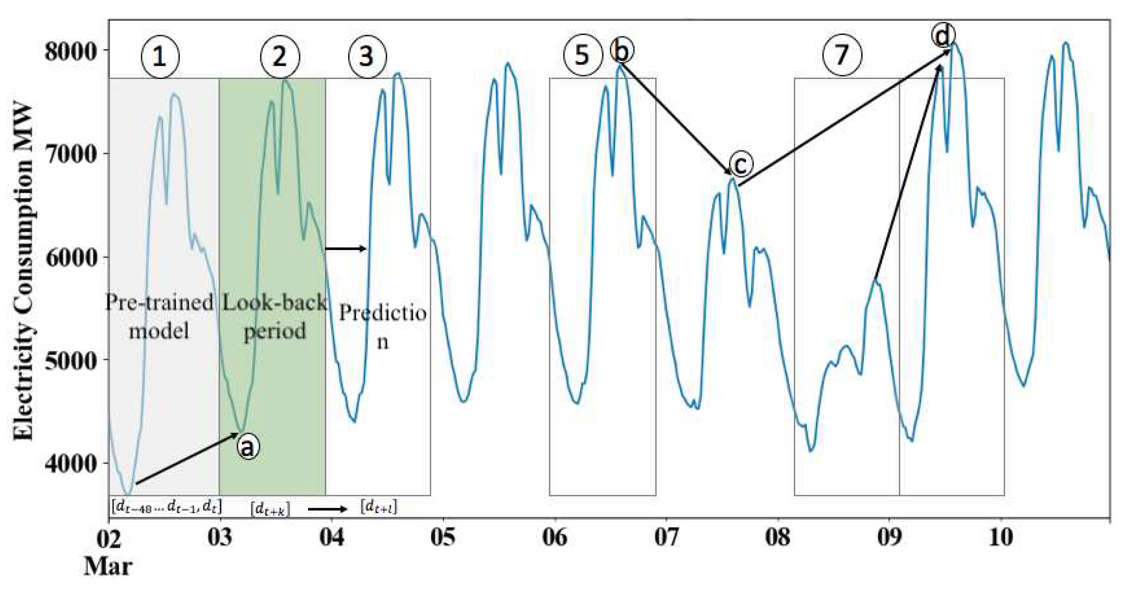
Figure 14.
Weekdays forecast using FNN.
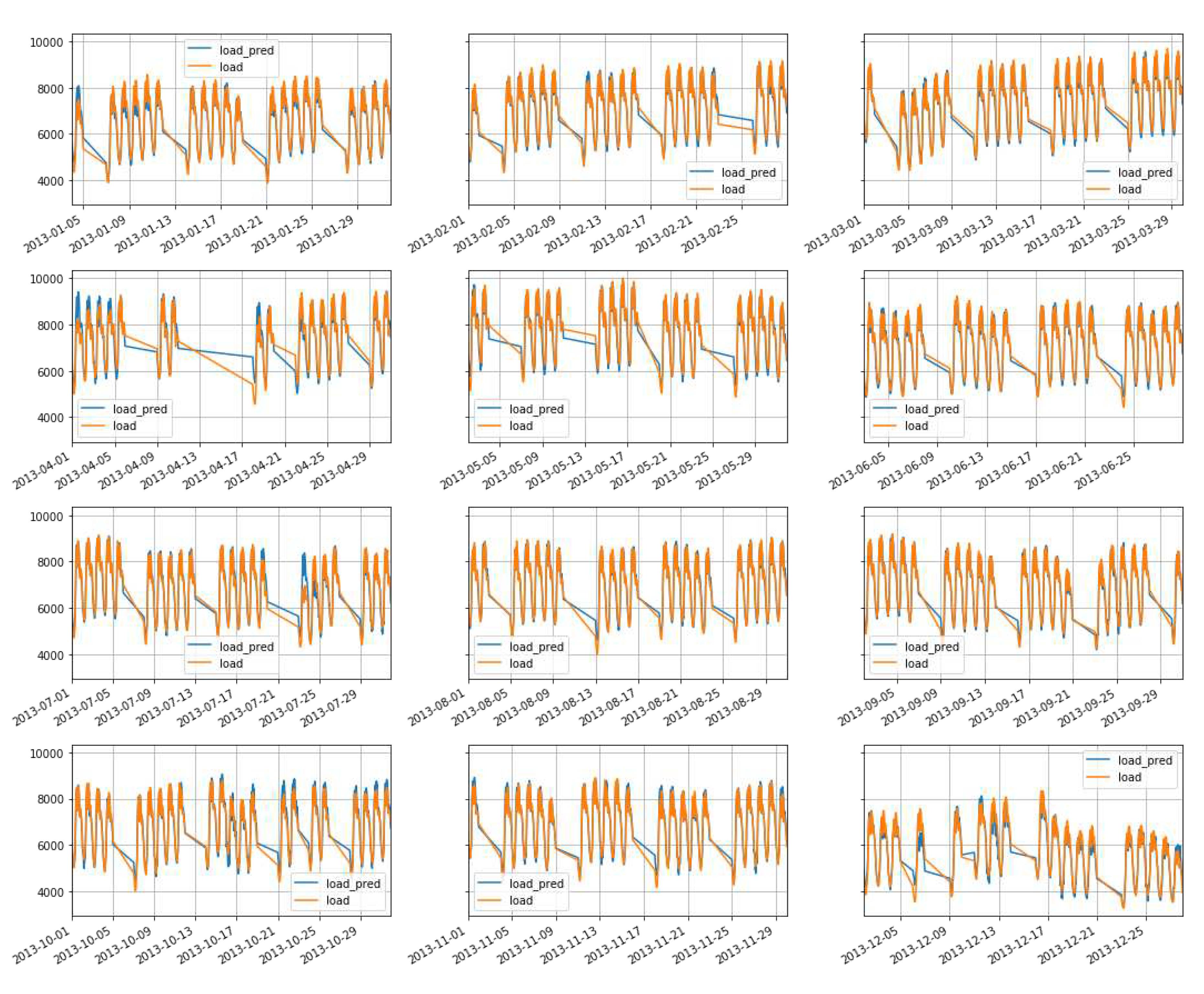
Figure 15.
Weekdays forecast using RNN-LSTM
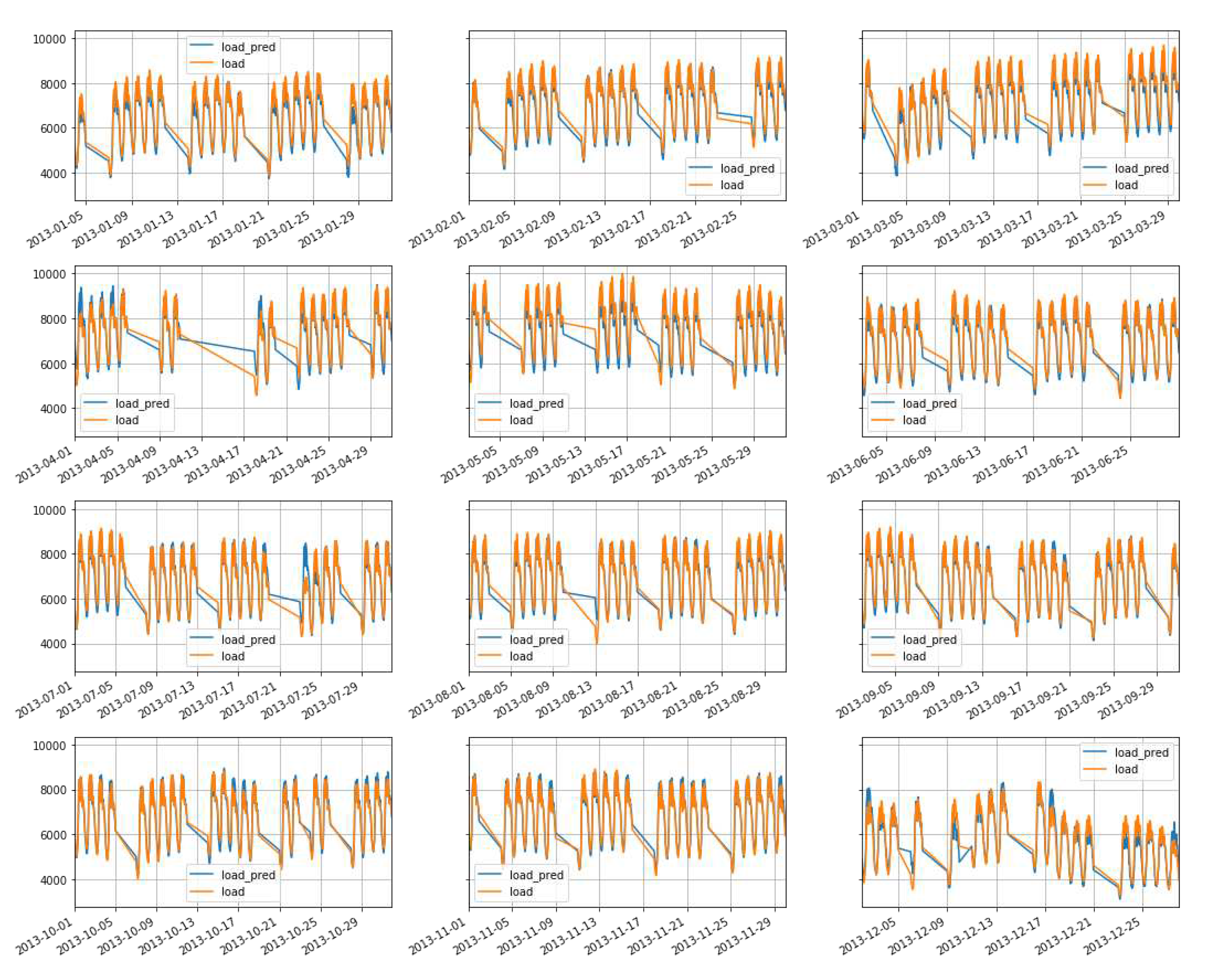
Figure 16.
Weekdays forecast using RNN-GRU
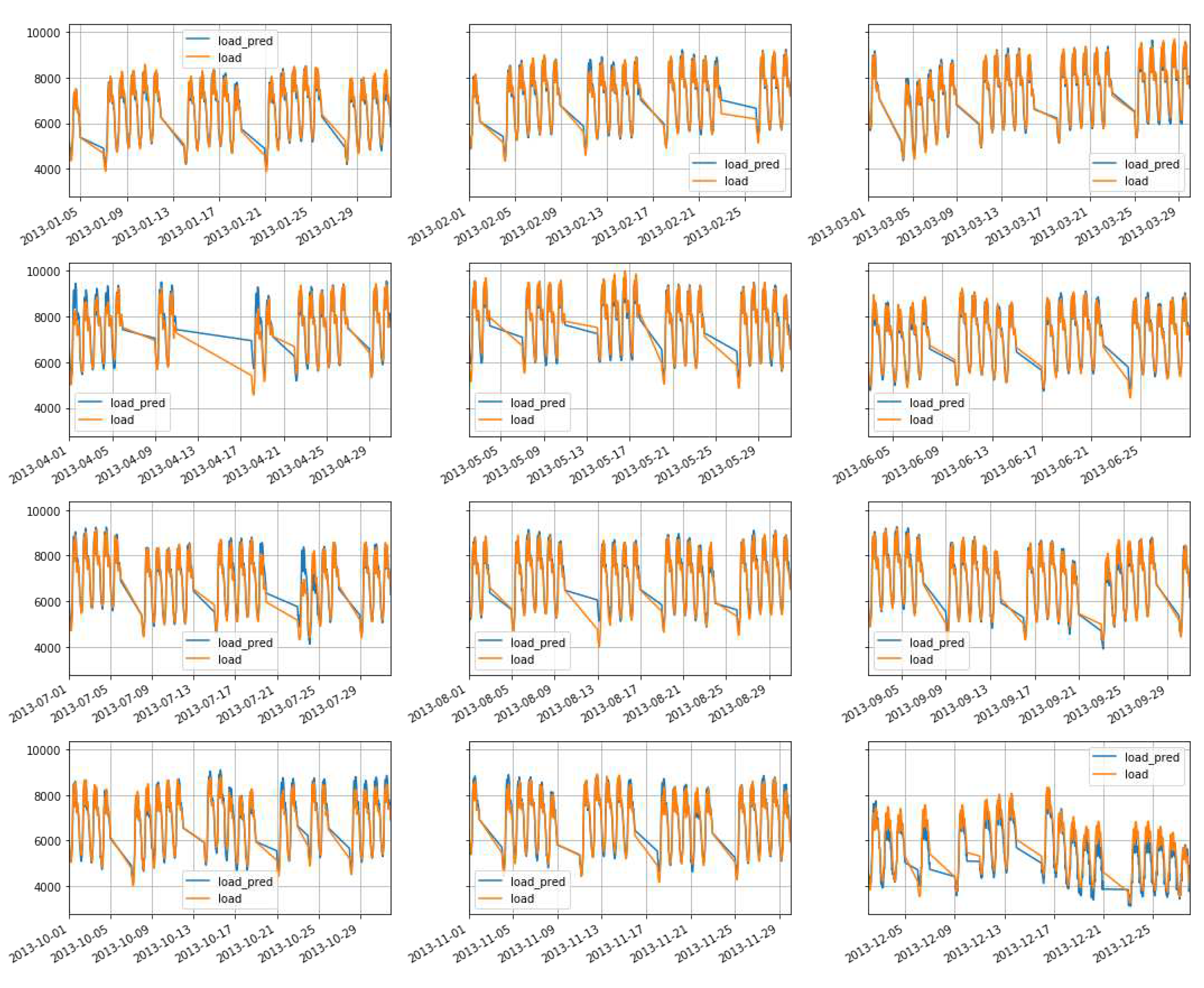
Figure 17.
Weekdays forecast using FNN using optimized parameters
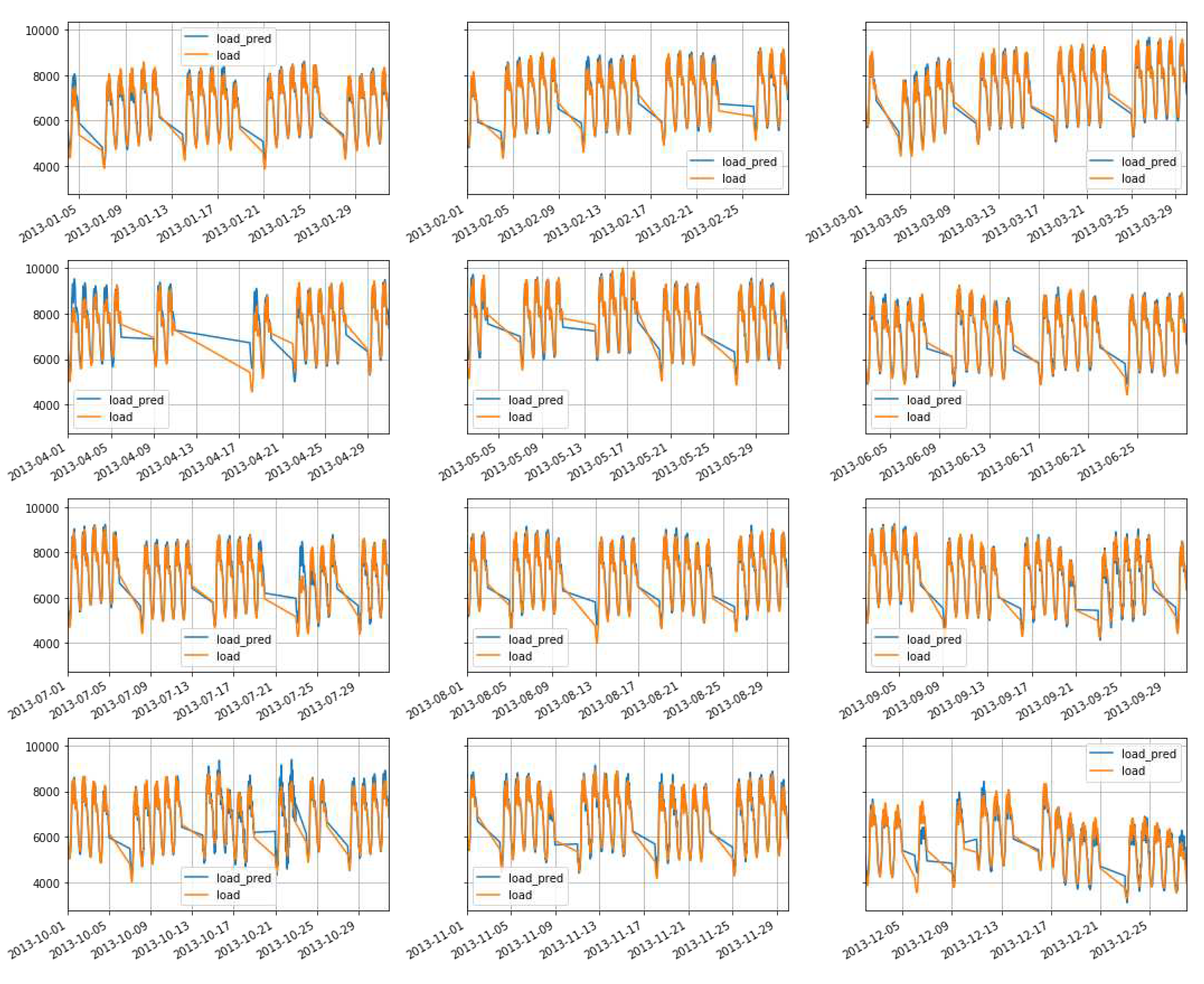
Table 1.
Variation of prediction accuracy due to the uncertainty nature of demand dataset.
| Model | MAPE | Prediction horizon |
Data source | Published year | Reference |
| ANN model | 2.90% | 1hr | DSO, Delhi, India | 2018 | Selvi et al. [16] |
| 1.96% | 1hr | Bandar Abbas, Iran | 2012 | Torabi et al. [22] | |
| CNN-LSTM | 2.02% | 1hr | Public dataset, England,USA | 2019 | Pramono et.al. [23] |
| 34.84% | 1hr | UCI ML dataset (households) | 2019 | Kim et al. [24] | |
| 1% | 24hr | Industrial area, China | 2020 | Qi et al. [25] |
Table 2.
List of published work based on 2009-2013 EGAT dataset[37].
Table 2.
List of published work based on 2009-2013 EGAT dataset[37].
| Method | Result | Reference |
| MLR with AR(2) | Bayesian estimation provides consistent and better accuracy compared to OLS estimation | [32] |
| PSO with ANN | Implementing PSO on ANN model outperformed shallow ANN model | [46] |
| OLS | Interation of variable improves the prediction accuracy | [31] |
| OLS and Bayesian estimation | Including temperature variable in a model can improved the prediction accuracy upto 20% | [45] |
| PSO & GA with ANN | PSO+GA outperformed PSO with ANN | [35] |
| OLS, GLSAR, FF-ANN | OLS and GLSAR models showed better forecasting accuracy than FF-ANN | [36] |
| Ensemble for regression and ML | Lowers the test MAPE implementing blocked Cross Validation scheme. | [37] |
| FNN, RNN based LSTM & GRU | For weekdays and for aggregate data GRU shows better accuracy | In this study |
Table 3.
List of selected input variables.
| Types | Variables | Description |
| Deterministic | WD | Week dummy [Mon <Tue ... <Sat<Sun] |
| MD | Month dummy [Feb <Mar <... <Nov <Dec] | |
| DayAfterHoliday | Binary 0 or 1 | |
| DayAfterLongHoliday | Binary 0 or 1 | |
| DayAfterSongkran | Binary 0 or 1 | |
| DayAfterNewyear | Binary 0 or 1 | |
| Temperature | Temp | Forecasted temperature |
| MaxTemp | Maximum forecasted temperature | |
| Square temperature | Square of the forecasted temperature | |
| MA2pmTemp | Moving avearage of temperature at 2pm | |
| Lagged | load1d_cut2pm | 1 day ahead untill 2pm and 2 day ahead after 2pm load |
| load2d_cut2pm | 2 days ahead untill 2pm and 3 day ahead after 2pm load | |
| load3d_cut2pmR | 3 days ahead untill 2pm and 4 days ahead after 2pm load | |
| load4d_cut2pmR | 4 days ahead untill 2pm and 5 days ahead after 2pm load | |
| Interaction | WD:Temp | Interaction: week day dummy to temperature |
| MD:Temp | Interaction: month dummy to temperature | |
| WD:load1d_cut2pm | Interaction: week day dummy to load1d_cut2pm | |
| WD:load2d_cut2pm | Interaction: week day dummy to load2d_cut2pm |
Table 4.
Experimental hyper-parameters testing setup for FNN.
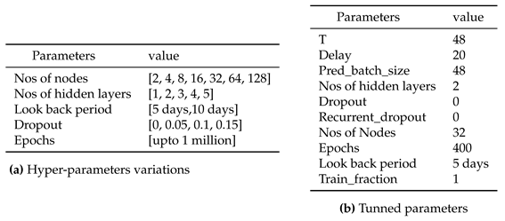 |
Table 7.
MAPE performance on the best parameters: day ahead forecast.
| Daytype | FNN | GRU | LSTM |
| non-holiday weekdays | 2.97 | 2.71 | 3.76 |
| non-holiday weekends | 3.83 | 4.62 | 3.58 |
| holidays | 9.79 | 6.70 | 6.96 |
| Overall | 3.54 | 3.44 | 3.86 |
Disclaimer/Publisher’s Note: The statements, opinions and data contained in all publications are solely those of the individual author(s) and contributor(s) and not of MDPI and/or the editor(s). MDPI and/or the editor(s) disclaim responsibility for any injury to people or property resulting from any ideas, methods, instructions or products referred to in the content. |
© 2023 by the authors. Licensee MDPI, Basel, Switzerland. This article is an open access article distributed under the terms and conditions of the Creative Commons Attribution (CC BY) license (http://creativecommons.org/licenses/by/4.0/).
Copyright: This open access article is published under a Creative Commons CC BY 4.0 license, which permit the free download, distribution, and reuse, provided that the author and preprint are cited in any reuse.


