<strong></strong>Geometrized Vacuum Physics. Part II. Algebra of Signatures

Mikhail Batanov-Gaukhman

doi:10.20944/preprints202307.0716.v1

Submitted:

09 July 2023

Posted:

12 July 2023

You are already at the latest version

Abstract

This article is the second part of a scientific project under the general name "Geometrized vacuum physics". On the basis of the Algebra of Stignatures presented in the previous article [1], this article develops the main provisions of the Algebra of Signatures. Both of the above algebras are aimed at studying the properties of an ideal vacuum, but at the same time they are universal and can be applied in various branches of knowledge. It is shown that the signature of a quadratic form is related to the topology of the metric space for which the given quadratic form is a metric. Conditions are given under which an additive imposition of metric spaces with different topologies (or signatures) leads to a total Ricci flat space similar to a Calabi-Yau manifold. A spin-tensor representation of metrics with different signatures is considered and a Dirac bundle of quadratic forms is presented. This article does not contain physical applications of the Algebra of Signatures, but the potential power of this mathematical apparatus will be demonstrated in subsequent articles of this project.

Keywords:

vacuum

;

geometrized vacuum physics

;

signature

;

algebra of signature

Subject:

Physical Sciences - Theoretical Physics

1. Introduction

This article is the second of a series of articles under the general title "Geometrized vacuum physics ", and is devoted to the presentation of the foundations of the Algebra of signatures.

In the first article [1], a local volume of ideal vacuum was considered, in which, by means of probing with mutually perpendicular light rays with a wavelength λ_m_,n (from the subrange Δλ = 10^m÷ 10ⁿcm), a 3D_m_,n-cubic lattice was obtained (see Figure 1, or Figure 5 in [1])

Figure 1. Non-curved 3D light lattice of λ_m_,n-vacuum, revealed from the "vacuum" (emptiness) by means of mutually perpendicular monochromatic rays of light with a wavelength λ_m_,n. The cells of such a lattice are cubes with edge length ε _m_÷n ~ 10²·λ_m_,n.

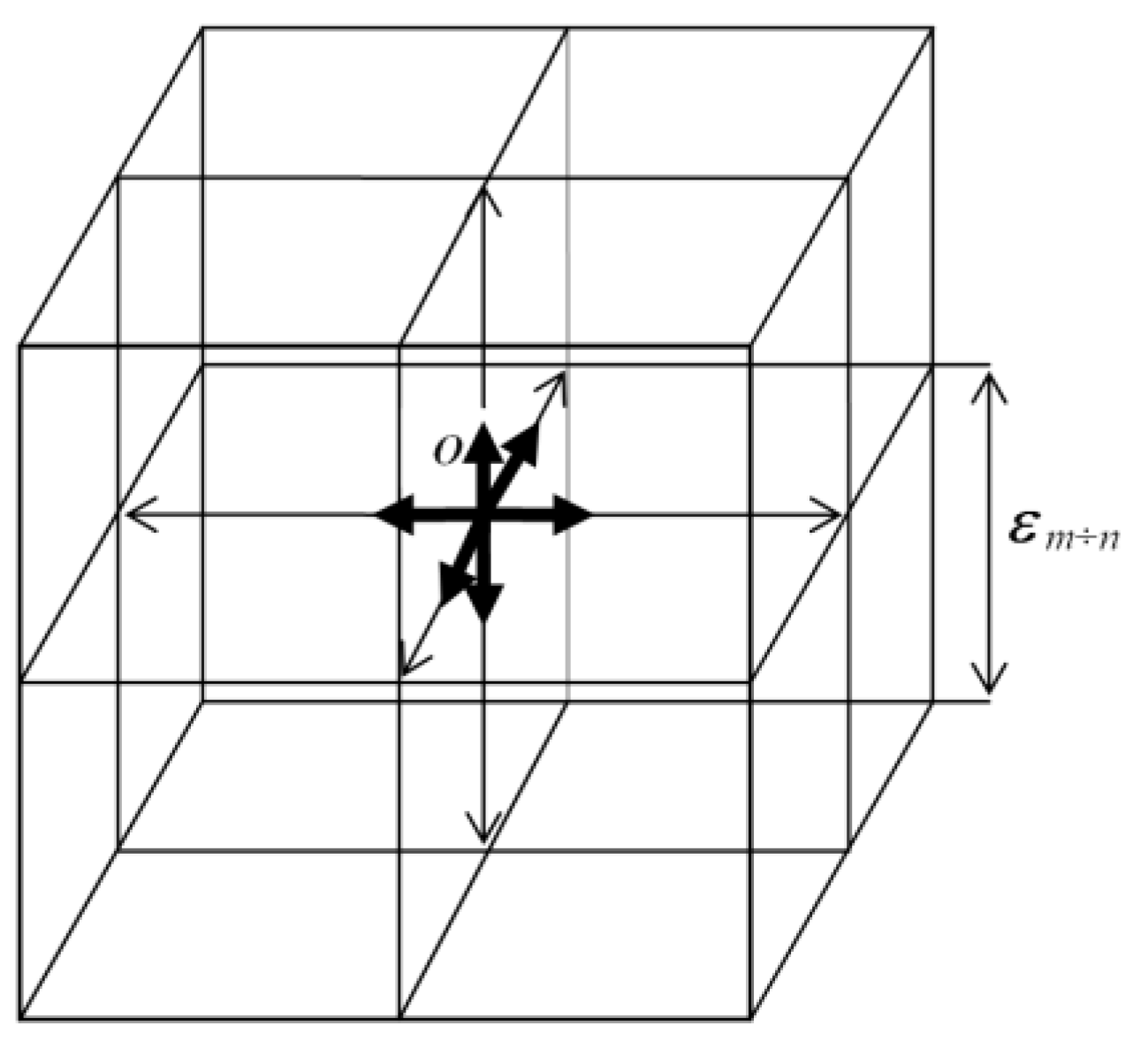
The three-dimensional extent revealed from the void using such a luminous 3D_m_,ncubic lattice is called in [1] λ_m_,n-vacuum or 3D_m_,n-landscape.

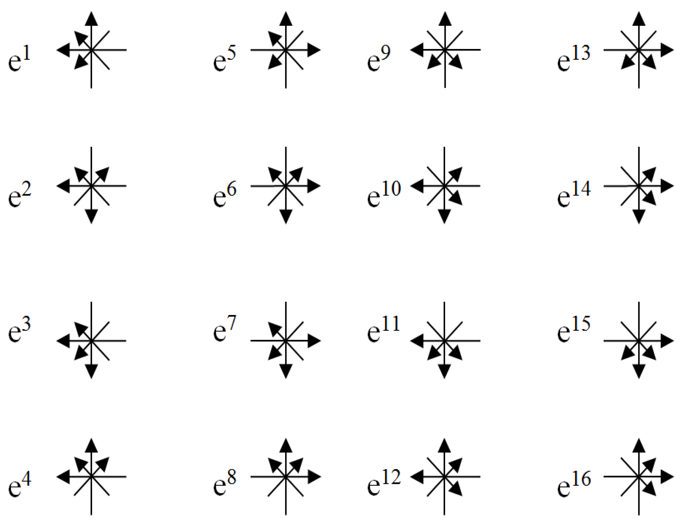
In § 3 of the article [1], it was found that the number of orthogonal 3-bases that originate at the central point O (see Figure 1), taking into account the direction of the time axis, is 16

3-bases shown in Figure 2 correspond to sixteen types of affine spaces that can be characterized by the corresponding signatures (see §4 and Table 1 in [1]). These sixteen stignatures of affine spaces form the stignature matrix (3) in [1]:

s t i g n (e_{i}^{(a)}) = (\begin{matrix} \{+ + + +\} & \{+ + + -\} & \{- + + -\} & \{+ + - +\} \\ \{- - - +\} & \{- + + +\} & \{- - + +\} & \{- + - +\} \\ \{+ - - +\} & \{+ + - -\} & \{+ - - -\} & \{+ - + +\} \\ \{- - + -\} & \{+ - + -\} & \{- + - -\} & \{- - - -\} \end{matrix})

(2)

Some properties of this matrix and the foundation of the Algebra of stignatures are described in [1].

Figure 2. Sixteen 4-bases starting at point O [1].

In this article, a transition is made from sixteen affine spaces with stignatures (2), which originate at the point O, to 256 × 4 = 1024 metric spaces, which intersect at the same point, under the condition of the "vacuum balance".

The conditions of "vacuum (i.e. zero) balance" were formulated in the article [1,2]: "If something is born from a vacuum, it is necessarily in a mutually opposite form (particle – antiparticle, convexity – concavity, wave – anti-wave, etc.), and on average remains equal to zero".

Moreover, each metric space is characterized by the corresponding signature. The totality of these signatures forms a matrix of signatures, the property of which is investigated in this article.

Also, in this second part of the "Geometrized Vacuum Physics" the foundations of the Algebra of Signatures are laid, which can be applied in various branches of scientific knowledge.

Together, the Algebra of Stignatures and the Algebra of Signatures form a single universal mathematical apparatus that can serve as the basis for describing and explaining many physical phenomena that were previously difficult to comprehend. The application of this apparatus to solving various physical problems will be presented in the following articles of the proposed project.

2. Materials and Method

2.1 Transition from 16 affine spaces to 256 metric spaces

We pass from the sixteen affine spaces with 4-bases shown in Figure 2 and their corresponding signatures (2) to metric spaces.

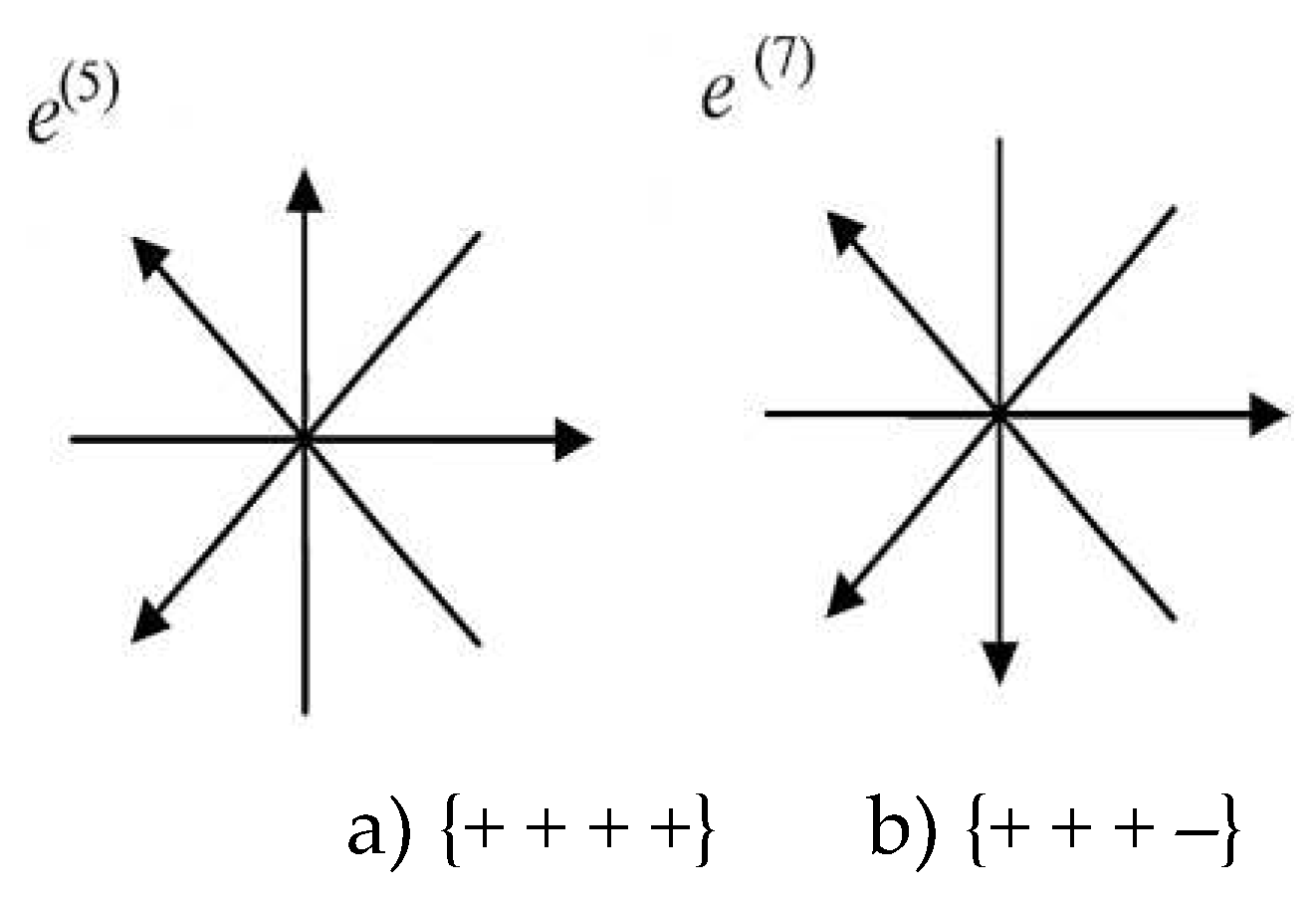
To do this, as an example, out of sixteen 4-bases (see Figure 2), we choose the 4-basis e_i⁽⁷⁾(e₀⁽⁷⁾,e₁⁽⁷⁾,e₂⁽⁷⁾,e₃⁽⁷⁾) with signature {+ + + –} and 4-basis e_i⁽⁵⁾(e₀⁽⁵⁾, e₁⁽⁵⁾, e₂⁽⁵⁾, e₃⁽⁵⁾) with signature {+ + + +} (see Figure 3)

Figure 3. Two 4-bases with different stignatures.

Let’s define two 4-vectors in affine spaces with 4-bases e_i⁽⁵⁾ and e_i⁽⁷⁾

ds⁽⁷⁾ = e_i⁽⁷⁾dx_i⁽⁷⁾ = e₀⁽⁷⁾dx₀⁽⁷⁾ + e₁⁽⁷⁾dx₁⁽⁷⁾ + e₂⁽⁷⁾dx₂⁽⁷⁾ + e₃⁽⁷⁾dx₃⁽⁷⁾,

(3)

ds⁽⁵⁾ = e_i⁽⁵⁾dx_i⁽⁵⁾ = e₀⁽⁵⁾dx₀⁽⁵⁾ + e₁⁽⁵⁾dx₁⁽⁵⁾ + e₂⁽⁵⁾dx₂⁽⁵⁾ + e₃⁽⁵⁾dx₃⁽⁵⁾,

(4)

where dx_i^(k) is the i-th projection of the 4-vector ds^(k) onto the x_i^(k) axis, whose direction is determined by the basis vector e_i^(k).

Let’s find the scalar product of 4-vectors (48) and (49)

ds^{(5,7) 2} = ds⁽⁵⁾ds⁽⁷⁾ = e_i⁽⁵⁾e_j⁽⁷⁾dxⁱ dx^j =
= e₀⁽⁵⁾e₀⁽⁷⁾dx₀dx₀ + e₁⁽⁵⁾e₀⁽⁷⁾dx₁dx₀ + e₂⁽⁵⁾e₀⁽⁷⁾dx₂dx₀ + e₃⁽⁵⁾e₀⁽⁷⁾dx₃dx₀ +
+ e₀⁽⁵⁾e₁⁽⁷⁾dx₀dx₁ + e₁⁽⁵⁾e₁⁽⁷⁾dx₁dx₁ + e₂⁽⁵⁾e₁⁽⁷⁾dx₂dx₁ + e₃⁽⁵⁾e₁⁽⁷⁾dx₃dx₁ +
+ e₀⁽⁵⁾e₂⁽⁷⁾dx₀dx₂ + e₁⁽⁵⁾e₂⁽⁷⁾dx₁dx₂ + e₂⁽⁵⁾e₂⁽⁷⁾dx₂dx₂ + e₃⁽⁵⁾e₂⁽⁷⁾dx₃dx₂ +
+ e₀⁽⁵⁾e₃⁽⁷⁾dx₀dx₃ + e₁⁽⁵⁾e₃⁽⁷⁾dx₁dx₃ + e₂⁽⁵⁾e₃⁽⁷⁾dx₂dx₃ + e₃⁽⁵⁾e₃⁽⁷⁾dx₃dx₃.

(5)

For the case under consideration, the scalar products of basis vectors e_i⁽⁵⁾e_j⁽⁷⁾ are:

for i = j e₀⁽⁵⁾e ₀⁽⁷⁾ = 1, e₁⁽⁵⁾e₁⁽⁷⁾ = 1, e₂⁽⁵⁾e₂⁽⁷⁾ = 1, e₃⁽⁵⁾e₃⁽⁷⁾ = –1,

(6)

for i ≠ j all e_i⁽⁵⁾e_j⁽⁷⁾= 0.

In this case, Ex. (5) becomes the quadratic form

ds^(5,7)2 = dx₀dx₀ + dx₁dx₁ + dx₂dx₂ – dx₃dx₃ = dx₀² + dx₁² + dx₂² – dx₃² , with signature (+ + + –).

(7)

Recall that the "signature" (the term of general relativity) is an ordered set of signs in front of the corresponding terms of the quadratic form.

To determine the signature of a metric space with metric (7), instead of performing the scalar product of vectors (5), it suffices to multiply the signs of the signatures of the 4-bases shown in Fig. 3:

{+ + + +}
{+ + + –}
(+ + + –)_×

(8)

In the numerator of the rank (8), the multiplication of signs in each column is performed according to the rules

{+} × {+} = {+}; {–} × {+} = {–},

(9)

the result of such multiplication is written in the denominator (under the line) of the same column. The performance of actions according to these rules will be called rank multiplication.

Just as it was done with the vectors ds⁽⁵⁾and ds⁽⁷⁾ {see Exs. (3) – (9)}, we scalarly multiply vectors from all 16 affine spaces with 4-bases, shown in Figure 3. As a result, we obtain 16 × 16 = 256 metric 4-spaces with 4-metrics of the form

ds^(а,b)2 = e_i^(а)e_j^(b)dxⁱ^(а)dx^j^(b),

(10)

where a = 1, 2, 3, … , 16; b = 1, 2, 3, … , 16.

The signatures of these 16 × 16 = 256 metric 4-spaces can be determined, similarly to (8), by rank multiplications of the signs of the signatures of the corresponding affine spaces, for example:

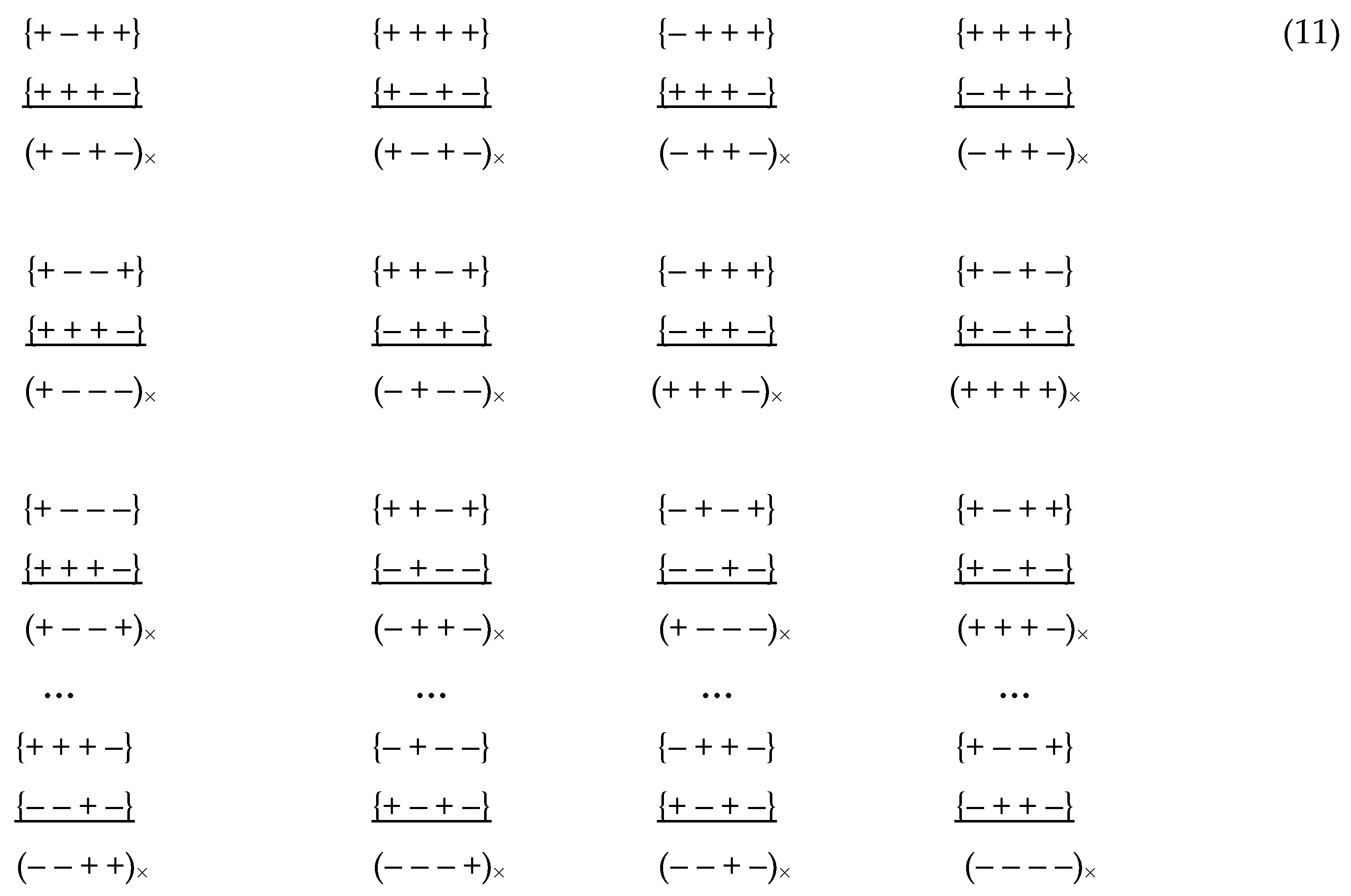
The point O (see Figure 1) is the intersection point of all 256 metric 4-spaces with 4-metrics (10) and the corresponding signature (11).

A set of 256 metric 4-spaces (4-maps) form a single 256-page "atlas" with a bonding point at point O, with a total number of mathematical measurements 256 × 4 = 1024.

The sum of all 256 4-metrics (10) intersecting at the point O is equal to zero

\sum_{k = 1}^{256} {d s}^{(k) 2} = \sum_{a = 1}^{16} \sum_{b = 1}^{16} e_{i}^{(a)} e_{j}^{(b)} {d x}^{i (a)} {d x}^{j (b)} = 0,

(12)

where k = 1,2,3,…,256 corresponds to one of 256 combinations a,b.

It is easy to verify that sum (12) is equal to zero, since among 256 × 4 = 1024 signs of all 256 signatures there are 512 {+} and 512 {–}. Thus, Ex. (12) satisfies the "vacuum balance" condition.

2.2 Four types of rank multiplication and division rules for different types of λ_m_,n-vacuums

Within the framework of the Algebra of Signatures, multiplication and division of signs in the numerators of ranks can be performed according to the following four types of arithmetic rules, which are assigned to four types of metric λ_m_,n-vacuums:

I - rules for commutative metric λ_m_,n-vacuum (or λ^I_m_,n-vacuum):

{+} × {+} = {+} {–} × {+} = {–}

(13)

{+} × {–} = {–} {–} × {–} = {+}

{+} : {+} = {+} {–} : {+} = {–}

(14)

{+} : {–} = {–} {–} : {–} = {+};

H - rules for non-commutative metric λ_m_,n-vacuum (or λ^H_m_,n-vacuum):

{+} × {+} = {+} {–} × {+} = {+}

(15)

{+} × {–} = {–} {–} × {–} = {+}

{+} : {+} = {+} {–} : {+} = {+}

(16)

{+} : {–} = {–} {–} : {–} = {+};

V - rules for the commutative metric λ_m_,n-antivacuum (or λ^V_m_,n-vacuum):

{+} × {+} = {–} {–} × {+} = {+}

(17)

{+} × {–} = {+} {–} × {–} = {–}

{+} : {+} = {–} {–} : {+} = {+}

(18)

{+} : {–} = {+} {–} : {–} = {–};

H' - rules for non-commutative metric λ_m_,n-antivacuum (or λ^H'_m_,n-vacuum):

{+} × {+} = {–} {–} × {+} = {–}

(19)

{+} × {–} = {+} {–} × {–} = {–}

{+} : {+} = {–} {–} : {+} = {–}

(20)

{+} : {–} = {+} {–} : {–} = {–}.

For example, let's write the ranking (8) and several other rankings from the list (11) for four types of λ_m_,n-vacuums with the corresponding multiplication rules (13), (15), (17), (19)

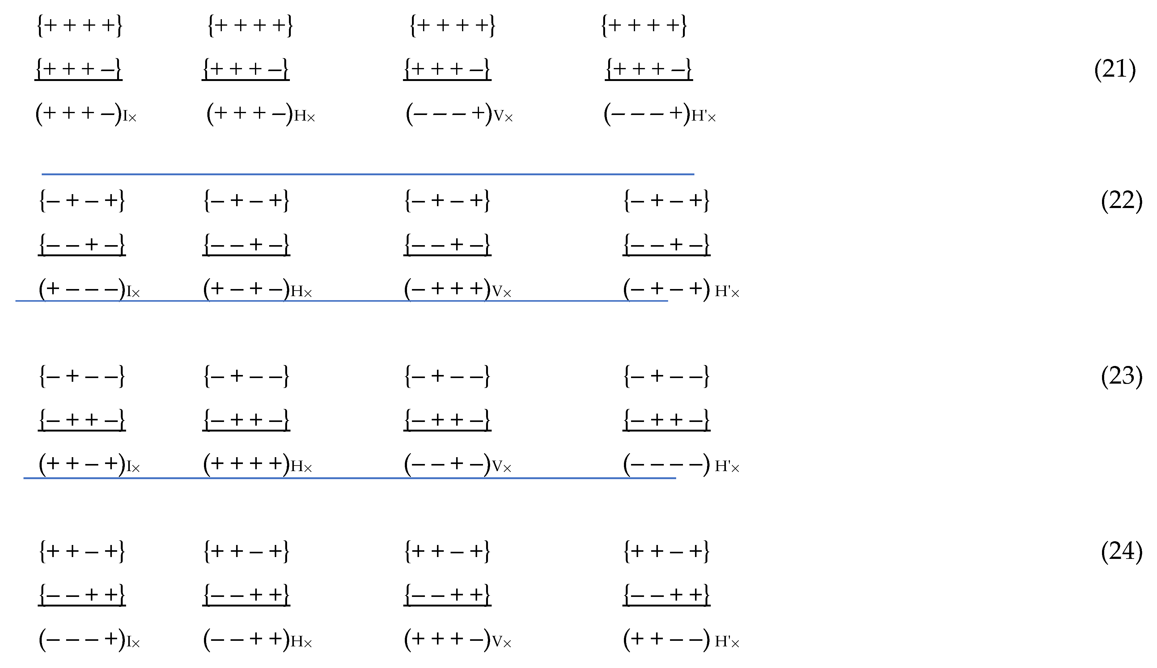
In this case, the sum of signs in the denominators of each quadruple of ranks (21) – (24) is equal to zero, for example, for four ranks (21) we have

(+ + + –) + (+ + + –) + (– – – +) + (– – – +) = 0,

(25)

and the sum of these signatures is equal to the zero signature

(+ + + –) + (+ + + –) + (– – – +) + (– – – +) = (0 0 0 0).

(26)

This corresponds to the "vacuum balance" condition.

Taking into account the four rules for multiplication of signs (13), (15), (17), (19), it turns out that at the point O under study (see Figure 1) four λ^L_m_,n-vacuums or 256 × 4 = 1024 metric spaces intersect, which are characterized by metrics (that is, quadratic forms)

{d s}^{(l) 2}

with the corresponding signatures.

The sum of all four metric λ^L_m_,n-vacuums and, accordingly, the sum of all 1024 metrics

{d s}^{(l) 2}

is still equal to zero

λ^I_m_,n-vacuum + λ^H_m_,n-vacuum + λ^V_m_,n-vacuum + λ ^H'_m_,n-vacuum = 0,

(27)

\sum_{l = 1}^{1024} {d s}^{(k) 2} = 0,

(28)

which satisfies the requirement of maintaining the "vacuum balance". The sum of metric λ^L_m_,n-vacuums (27) {or quadratic forms (28)} will also be called "deep zero".

Metric λ^L_m_,n-vacuums (27) are "supports" for each other and provide complete balancing of the metric emptiness. In what follows, each metric λ^L_m_,n-vacuum will be assigned a specific factorial of zero corresponding to one of the multiplication rules (13), (15), (17), (19):

0_I! = 1, 0_H! = –1, 0_V! = i, 0_H'! = – i.

(29)

so that the sum of these factorials corresponds to "true zero"

0_I! + 0_H! + 0_V! + 0_H'! = 1 + (–1) + i + (– i) = 0.

(30)

The identity of "deep zero" and "true zero" will lead to closed completeness of the developed theory.

2.3 Signature matrix

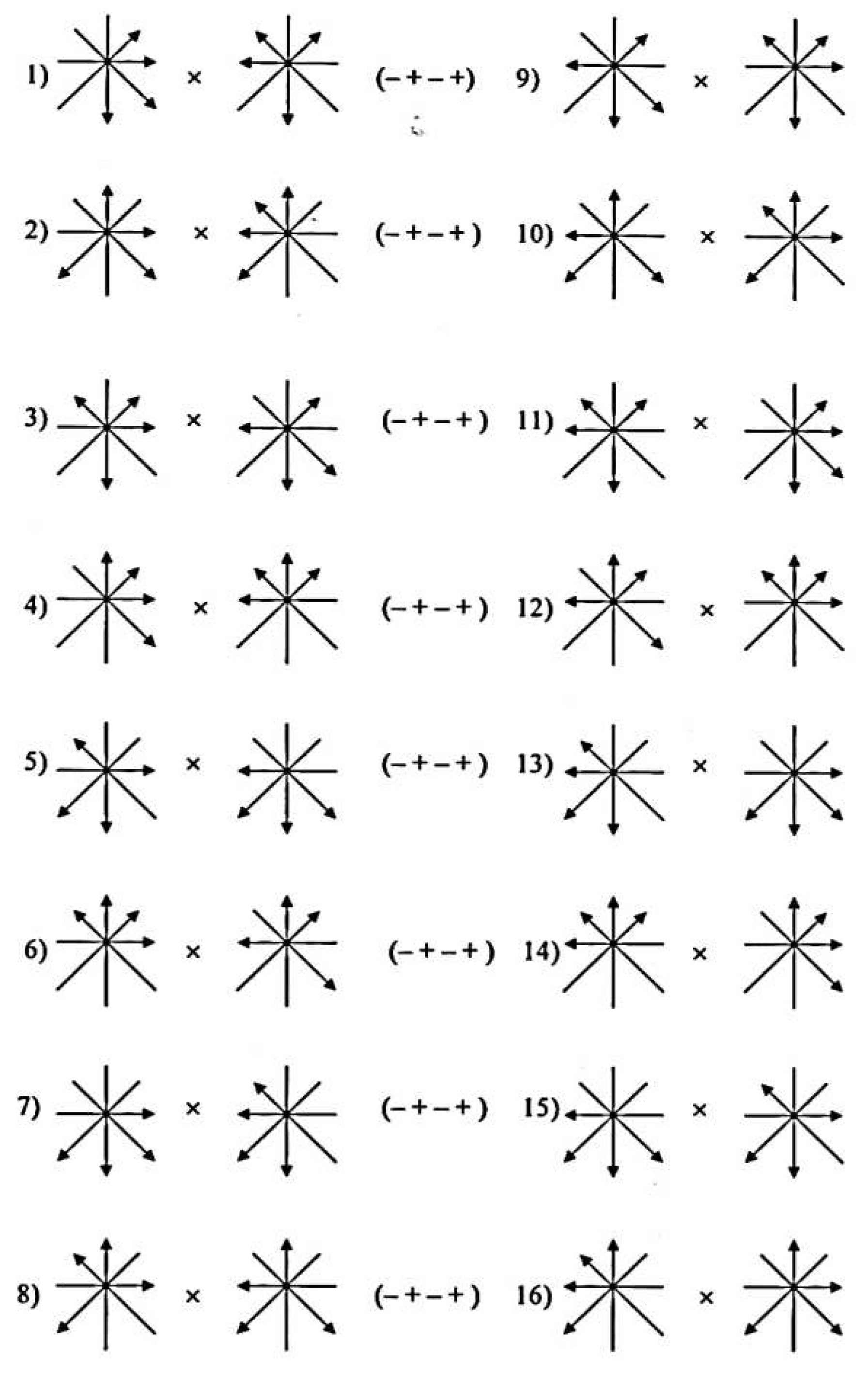
As shown above, the scalar multiplication of the sixteen 4-bases shown in Figure 2, with each other led to the formation of an atlas of 16 × 16 = 256 metric spaces with metrics (10) ds⁽^аb⁾²= e_i⁽^а⁾e_j^(b)dxⁱ⁽^а⁾dx^j^(b) with the corresponding signatures. However, there are only 16 different signatures, since there is a 16-fold degeneracy. For example, 16 scalar products of 4-bases shown in Figure 4 result in sixteen quadratic forms (i.e., metrics) with the same signature (– + – +):

Figure 4. Sixteen scalar products of 4-bases, resulting in to metrics with the same signature (– + – +).

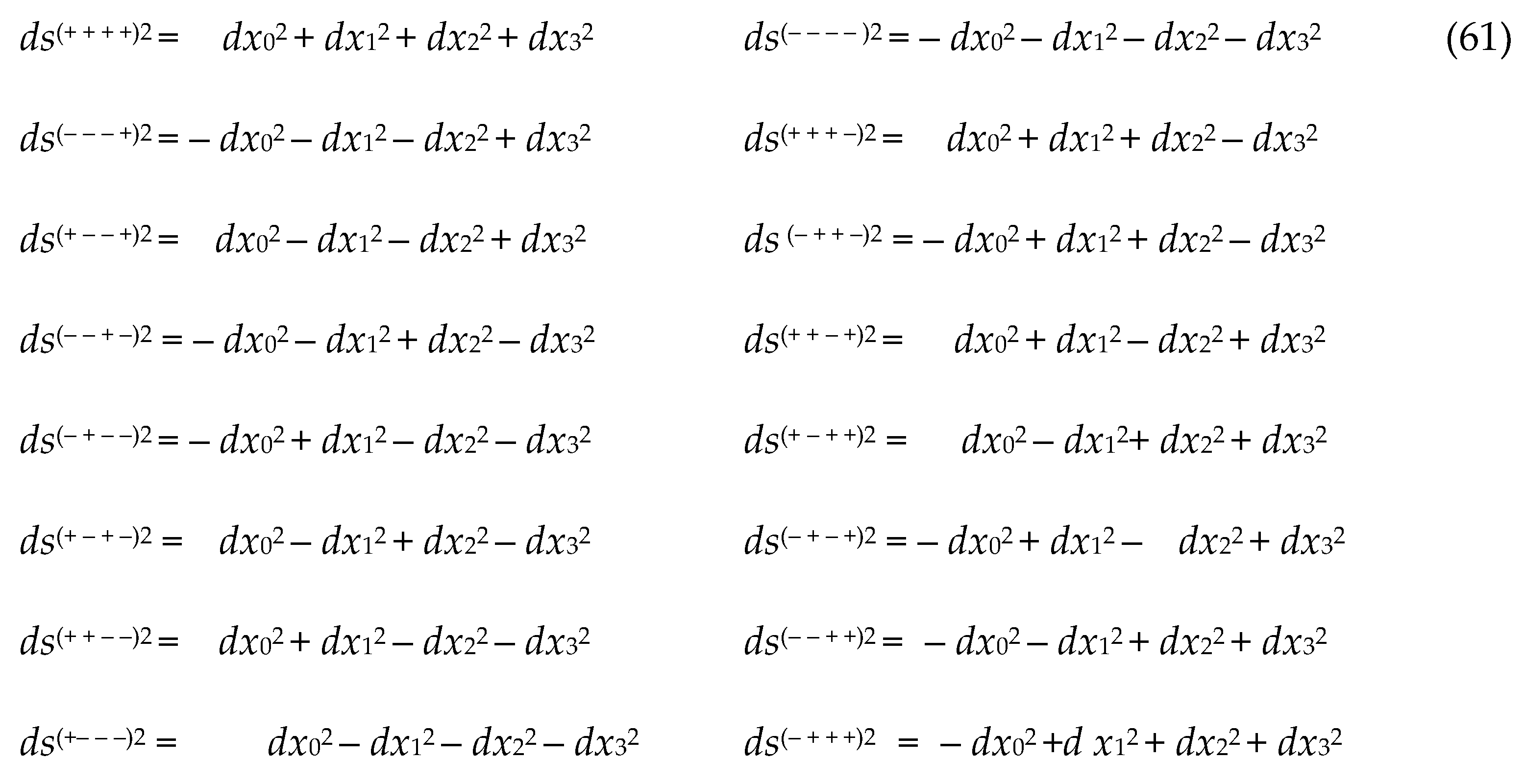
Similarly, we obtain 16-fold degeneracy with all other metric spaces. Thus, it is possible to single out only 256 : 16 = 16 types of metric 4-spaces with quadratic forms (i.e., metrics)

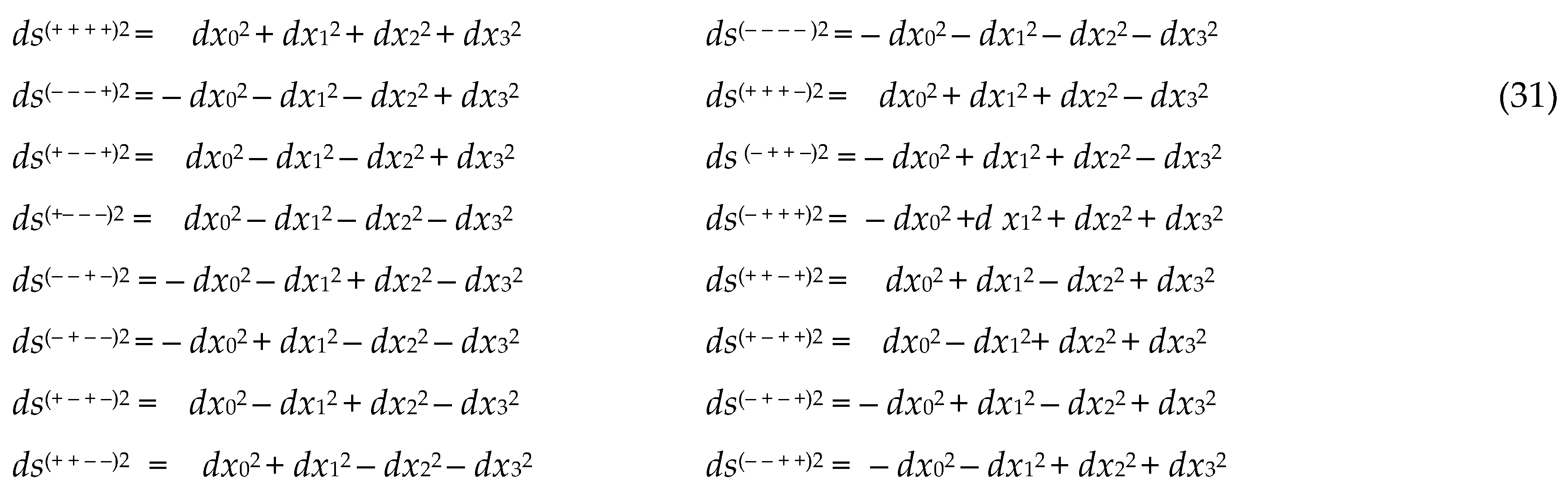
with the corresponding signatures, which form a matrix

s t i g n ({d s}^{(а, b) 2}) = (\begin{matrix} (+ + + +) & (+ + + -) & (- + + -) & (+ + - +) \\ (- - - +) & (- + + +) & (- - + +) & (- + - +) \\ (+ - - +) & (+ + - -) & (+ - - -) & (+ - + +) \\ (- - + -) & (+ - + -) & (- + - -) & (- - - -) \end{matrix}) .

(32)

The elements of the matrix of signatures (32) completely coincide with the elements of the matrix of signatures (2) {or (3) in the article [1]}. Therefore, the properties of the signature matrix (32) largely repeat the properties of the signature matrix (see [1]) in the next branch of the theory development.

2.4 Relationship between signature and 4-space topology

According to Felix Klein's classification [3], metric spaces with metrics (31) can be divided into three topological types:

1st type: 4-spaces whose signatures consist of four identical signs [3]:

x₀² + x₁² +x₂² +x₃² = 0 (+ + + +)

(33)

– x₀² – x₁² – x₂² – x₃² = 0 (– – – –)

are the so-called null metric 4-spaces. These "spaces" have only one real point, located at the beginning of the light cone. All other points of these extensions are imaginary. In fact, the first of the Exs. (33) describes not the “extent”, but a single point (or “white” point), and the second describes the only anti-point (or “black” point).

2nd type: 4-spaces whose signatures consist of two positive and two negative signs [3]:

x₀² – x₁² – x₂² + x₃² = 0 (+ – – +)

(34)

x₀² + x₁² – x₂² – x₃² = 0 (+ + – –)
x₀² – x₁² + x₂² – x₃² = 0 (+ – + –)
– x₀² + x₁² + x₂² – x₃² = 0 (– + + –)
– x₀² – x₁² + x₂² + x₃² = 0 (– – + +)
– x₀² + x₁² – x₂² + x₃² = 0 (– + – +)

are different variants of 4-dimensional tori.

3rd type: 4-spaces whose signatures consist of three identical signs and one opposite one [3]:

– x₀² – x₁² – x₂² + x₃² = 0 (– – – +)

(35)

– x₀² – x₁² + x₂² – x₃² = 0 (– – + –)
– x₀² + x₁² – x₂² – x₃² = 0 (– + – –)
x₀² – x₁² – x₂² – x₃² = 0 (+ – – –)
x₀² + x₁² + x₂² – x₃² = 0 (+ + + –)
x₀² + x₁² – x₂² + x₃² = 0 (+ + – +)
x₀² – x₁² + x₂² + x₃² = 0 (+ – + +)
– x₀² + x₁² + x₂² + x₃² = 0 (– + + +)

are oval 4-surfaces: ellipsoids, elliptic paraboloids, two-sheeted hyperboloids.

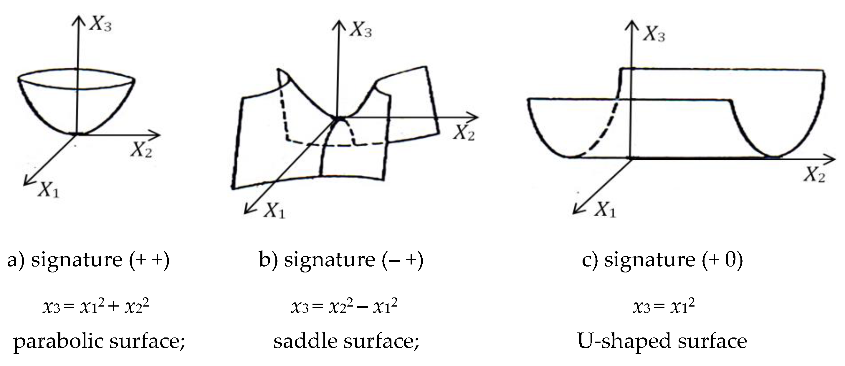
A simplified illustration of the connection between the signature of a 2-dimensional space and its topology is shown in Figure 5. This figure shows that the signature of the quadratic form is uniquely related to the topology of the 2-dimensional extent. But not vice versa, the extension topology is a much more capacious concept than the signature of its metric.

Figure 5. Illustration of the connection between the signature of a 2-dimensional space and its topology [3].

2.5 Splitting the metric zero

The sum of all 16 metrics (31) is zero:

ds_Σ² = ds^{(+– – –)2} + ds^{(+ + + +)2} + ds^{(– – – +)2} + ds^{(+ – – +)2} +

+ ds^{(– – + –)2} + ds^{(+ + – –)2} + ds^{(– + – –)2} + ds^{(+ – + –)2} +

(36)

+ ds^{(– + + +)2} + ds^{(– – – – )2} + ds^{(+ + + –)2} + ds ^{(– + + –)2} +
+ ds^{(+ + – +)2} + ds^{(– – + +)2} + ds^{(+ – + +)2} + ds^{(– + – +)2} = 0.

Indeed, summing metrics (31), we obtain

ds_Σ² = (dx₀dx₀ – dx₁dx₁ – dx₂dx₂ – dx₃dx₃) + (dx₀dx₀ + dx₁dx₁ + dx₂dx₂ + dx₃dx₃) +

(37)

+ (– dx₀dx₀ – dx₁dx₁ + dx₂dx₂ – dx₃dx₃) + (dx₀dx₀ – dx₁dx₁ – dx₂dx₂ + dx₃dx₃) +
+ (– dx₀dx₀ – dx₁dx₁ + dx₂dx₂ – dx₃dx₃) + (dx₀dx₀ + dx₁dx₁ – dx₂dx₂ – dx₃dx₃) +
+ (– dx₀dx₀ + dx₁dx₁ – dx₂dx₂ – dx₃dx₃) + (dx₀dx₀ – dx₁dx₁ + dx₂dx₂ – dx₃dx₃ ) +
+ (– dx₀dx₀ + dx₁dx₁ + dx₂dx₂ + dx₃dx₃) + (– dx₀dx₀ –dx₁dx₁– dx₂dx₂ –dx₃dx₃) +
+ (dx₀dx₀ + dx₁dx₁ + dx₂dx₂ – dx₃dx₃) + (– dx₀dx₀ +dx₁dx₁ +dx₂dx₂ – dx₃dx₃) +
+ (dx₀dx₀ + dx₁dx₁ – dx₂dx₂ + dx₃dx₃) + (– dx₀dx₀ – dx₁dx₁+ dx₂dx₂ +dx₃dx₃) +
+ (dx₀dx₀ – dx₁dx₁ + dx₂dx₂ + dx₃dx₃) + (– dx₀dx₀ + dx₁dx₁ –dx₂dx₂ +dx₃dx₃) = 0.

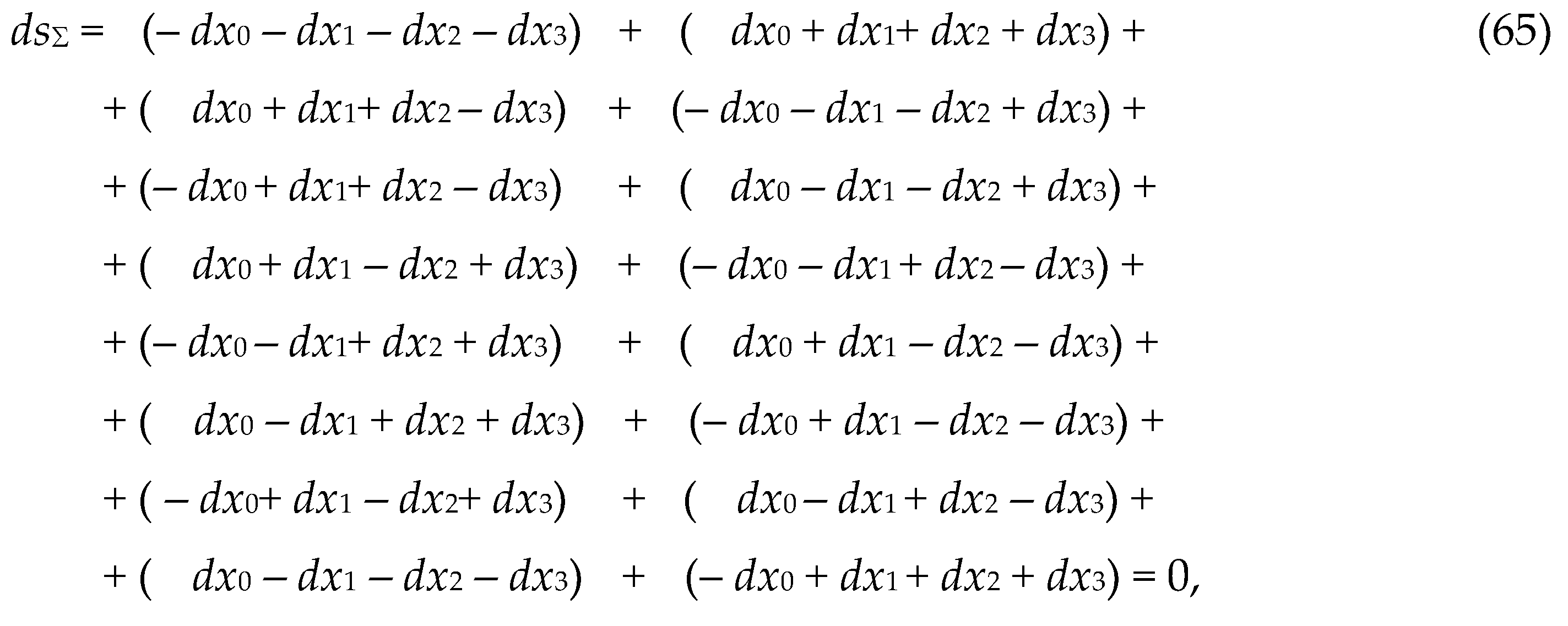
Instead of summing homogeneous terms in Ex. (37), only the signs in front of these terms can be summed. Therefore, the total metric (37) can be represented as a ranking expression:

where the summation (or subtraction) of signs is carried out according to the rules:

(+) + (+) = 2(+), (–) + (+) = (0), (+) – (+) = (0), (–) – (+) = 2(–),

(39)

(+) + (–) = (0), (–) + (–) = 2(–), (+) – (–) = 2(+), (–) – (–) = (0).

The sum of the signs, both in the columns of the ranks (38) and in their lines between the ranks, is equal to zero. Therefore, this ranking identity will be called the "splitting of the metric zero".

2.6 Operations with ranks

The ranking expression (38) makes it possible to perform some operations in the vicinity of the investigated point O (see Figure 1) without violating the “vacuum balance”. Such operations include, for example, the symmetrical transfer of the first and last columns to the other side of equality with sign inversion, while observing line-by-line and column-by-column vacuum balance:

Similarly, any columns of the rank expression (38) can be symmetrically transferred to the other side like (40).

It is possible to transfer any string from the numerators of the rankings (38) to their denominators, also with the inversion of signs, and observing the line-by-line vacuum balance, for example:

Mixed line and column transfer operations are also possible, which do not violate the conditions of line-by-line vacuum balance, for example

Such a ranking operations correspond to certain vacuum symmetries, which will be considered in the following articles of the proposed project.

2.7 Bilateral metric space

We transfer the signatures (– + + +) and (+ – – –) from the numerators of the ranks (38) to their denominators

In expanded form, the ranks (43) have the following form

The ranking expression (44) is equivalent to the fact that the addition (i.e., additive overlay) of 7-metric spaces with signatures (topologies) indicated in the numerator of the left ranking (43) form a metric Minkowski 4-space with the metric

ds^{(+ – – –)2} = c²dt² – dx² – dy² – dz² = dx₀² – dx₁² – dx₂² – dx₃² with signature (+ – – –),

(44)

where ds^{(+ – – –)2} = ds^{(+ + + +)2} + ds^{(– – – +)2} + ds^{(+ – – +)2} + ds^{(– – + –)2} + ds^{(+ + – –)2} + ds ^{(– + – –)2} + ds^{(+ – + –)2},

(45)

this Minkowski 4-space will be conditionally called the outer side of the λ_m_,n-vacuum (or subcont – short for “substantial continuum”).

In this case, the additive imposition of 7 metric spaces with signatures indicated in the numerator of the right-th rank (43) forms a metric Minkowski 4-antispace with the metric

ds^{(– + + +)2} = – c²dt² + dx² + dy² + dz² = – dx₀² + dx₁² + dx₂² + dx₃² with signature (– + + +),

(46)

where ds^{(– + + +)2} = ds^{(– – – – )2} + ds^{(+ + + –)2} + ds^{(– + + –)2} + ds^{(+ + – +)2} + ds^{(– – + +)2} + ds^{(+ – + +)2} + ds^{(– + – +)2}.

(47)

This metric Minkowski 4-antispace will be conditionally called the inner side of the λ_m_,n-vacuum (or antisubcont – short for “antisubstantial continuum”.

The concepts of "subcont" and "antisubcont" are mental constructions that are intended only to create the illusion of "visibility" of two adjacent mutually opposite sides of one λ_m_,n-vacuum. If one side of a sheet of paper is painted blue, and the other side of the same sheet is painted red, then the blue side of the sheet can be associated with the “subcont”, and its red side with the “antisubcont”. The concepts of "subcont" and "antisubcont" are introduced only to facilitate the visualization of intra-vacuum processes, but they have nothing to do with reality. However, as will be shown in the following articles of this project, using these mental concepts it is possible to inspire real vacuum effects.

The operation described by the ranking expression (43) allows you to mentally “reveal” from the void the two-sided λ_m_,n-vacuum with the number of mathematical dimensions 4 + 4 = 8 = 2³. We propose to call such a two-sided 8-dimensional space 2³-λ_m_,n-vacuum, provided that the 2³-λ_m_,n-vacuum balance is maintained

ds^{(+ – – –)2} + ds^{(– + + +)2} = 0,

(48)

with ranking equivalent (+ – – –) + (– + + +) = (0 0 0 0), or in transposed form

(+ – – –)

(49)

(– + + +)
(0 0 0 0)₊

In the terminology proposed here, the ranking expression (38) is equivalent to the balance condition for a 2⁶-λ_m_,n-vacuum with 4-dimensional sides (or faces), since the number of mathematical dimensions of such a 16-faced extension:

4 × 16 = 64 = 2⁶.

(50)

Philosophical understanding of the ranking expression (38) can lead to the roots of religious and mythological traditions, where the number 7 has the sacred meaning of "Seven Heavens", and two mutually opposite sides of the 2³-λ_m,n-vacuum corresponds to the perception of reality through ascending logic to the Hegelian dialectic.

Here, for the first time, mathematical (speculative) calculations of the Algebra of Signature led to the following very important practical conclusion. The vacuum balance condition led to the need to assume that the empty extent surrounding us has at least sixteen 4-dimensional "faces" with signatures (32). At the same time, in some cases, the number of faces of such an empty extent can be reduced to two with signatures (+ – – –) and (– + + +), and in a number of other problems it can be increased to infinity (see section 9).

In other words, it is necessary to realize that the space around us has at least two sides: "external" and "internal", which can be conditionally called "subcont" and "antisubcont". This will require a full review of our speculative attitude to reality, but as it turns out below, one-sided theories inevitably lead to unsolvable paradoxes, and 16-sided (or at least two-sided) theories allow us to significantly expand the range of tasks to be solved.

Recall that in A. Einstein's General Relativity there is only one metric 4-space with a signature, for example, (+ – – –). Whereas in the geometrized vacuum physics developed here, based on the Algebra of Signatures, any λ_m_,n-vacuum can have at least two sides (i.e. mutually opposite metric 4-spaces): the outer side (or subcont) with signatures (+ – – –) and the inner side (or antisubcontent) with the signature (– + + +).

2.8 Binary triads

Not only the ranking expression (38) leads to the antipodal dyad: "4-space - 4-antispace" Minkowski with opposite signatures (+ – – –) and (– + + +). The following ranking expressions also lead to this dyad:

These ranking expressions (binary triads) also satisfy the vacuum balance condition and play an important role in "vacuum chromodynamics", which will be described in the following articles of this project.

2.9 Transverse bundle of λ_m_,n-vacuum

Like the ranking expression (41) and (43), any pair of metric 4-spaces with mutually opposite signatures can be represented as a sum of 7 + 7 = 14 metric extensions with other signatures.

For example, the conjugate pair of metrics ds^{(–
+ + –)2} and ds^{(+ – – +)2} with mutually opposite signatures (– + + –) and (+ – – +) can be expressed by summing (i.e., additive superposition) 7 + 7 = 14 metric 4-spaces with signatures

Similarly, out of 256 metrics with signatures (11), 256 : 2 = 128 conjugate pairs of metrics can be distinguished, each of which can be expressed in terms of an additive superposition of 7 + 7 = 14 metric 4-subspaces with corresponding signatures while maintaining a vacuum balance.

In turn, the conjugate pairs of 4-subspaces can be similarly decomposed into sums of 7 + 7 = 14 subspaces, and this can continue indefinitely.

It turns out that the light-geometry of the void is balanced with respect to zero, in which the "vacuum" is first represented as an infinite number of λ_m_,n-vacuums nested into each other (see § 1 and Figure 2 in the article [1]). This representation of emptiness is called the longitudinal stratification (bundle) of "vacuum". Then each λ_m_,n-vacuum splits into an infinite number of metric 4-subspaces, 4-sub-subspaces, and so on. with 16 types of signatures (or topologies, see § 4) without violating the vacuum balance. Such an infinite splitting of each λ_m_,n-vacuum will be called the transverse bundle of the "vacuum".

The longitudinal and transverse stratification (bundle) of the "vacuum" leads to the fact that at each point of the void (including the point O under study, see Figure 1) there is an additive imposition of an infinite number of metric 4-spaces with 16 types of signatures (i.e., topologies, among which are 6 types of tori (34) and 8 types of oval surfaces (35)), which completely compensate for each other's manifestations (i.e. 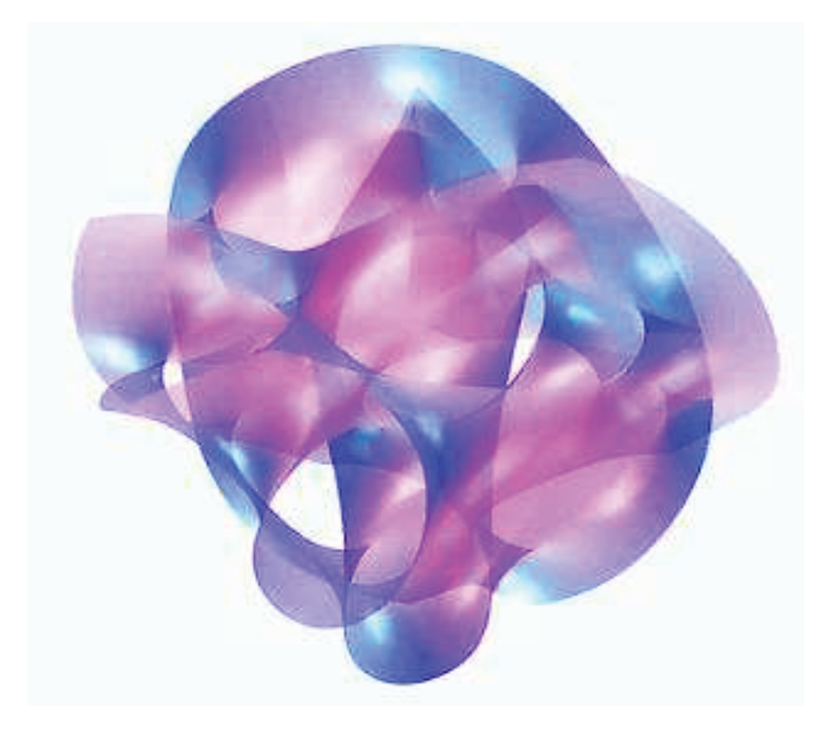the condition of "vacuum balance" is observed). This leads to the formation of a zero Ricci-flat space, which is in many ways similar to a compact Calabi-Yau manifold (i.e., a multidimensional complex torus) (see Figure 6).

Figure 6. One of the implementations of a 2D projection of a 3D visualization of a local area of a 10-dimensional Calabi-Yau manifold [4].

2.10 Spin-tensor representation of metrics with different signatures

Let’s consider the metric

ds^{(+ – – –)2} = dx₀² – dx₁² – dx₂² – dx₃² with signature (+ – – –).

(55)

For brevity, we omit the signs of the differentials in the metric (55)

s² = x₀²– x₁² – x₂² – x₃².

(56)

As is known, the quadratic form (56) is a determinant of the Hermitian 2×2-matrix

{(\begin{matrix} x_{0} + x_{3} & x_{1} + i x_{2} \\ x_{1} - i x_{2} & x_{0} - x_{3} \end{matrix})}_{d e t} = |\begin{matrix} x_{0} + x_{3} & x_{1} + i x_{2} \\ x_{1} - i x_{2} & x_{0} - x_{3} \end{matrix}| = x_{0}^{2} - x_{1}^{2} - x_{2}^{2} - x_{3}^{2} = 0 with signature (+ - - -) .

(57)

It is easy to verify that this matrix is Hermitian by direct calculation

{(\begin{matrix} x_{0} + x_{3} & x_{1} + i x_{2} \\ x_{1} - i x_{2} & x_{0} - x_{3} \end{matrix})}^{+} = (\begin{matrix} x_{0} + x_{3} & x_{1} + i x_{2} \\ x_{1} - i x_{2} & x_{0} - x_{3} \end{matrix}) .

(58)

In the theory of spinors, matrices of the form (58) are called second-rank mixed Hermitian spin-tensors [6].

Let’s represent 2×2-matrix (58) in expanded form

А_{4} = (\begin{matrix} x_{0} + x_{3} & x_{1} + i x_{2} \\ x_{1} - i x_{2} & x_{0} - x_{3} \end{matrix}) = x_{0} (\begin{matrix} 1 & 0 \\ 0 & 1 \end{matrix}) - x_{1} (\begin{matrix} 0 & - 1 \\ - 1 & 0 \end{matrix}) - x_{2} (\begin{matrix} 0 & - i \\ i & 0 \end{matrix}) - x_{3} (\begin{matrix} - 1 & 0 \\ 0 & 1 \end{matrix}),

(59)

where

σ_{0}^{(+ - - -)} = (\begin{matrix} 1 & 0 \\ 0 & 1 \end{matrix}); σ_{1}^{(+ - - -)} = (\begin{matrix} 0 & - 1 \\ - 1 & 0 \end{matrix}); σ_{2}^{(+ - - -)} = (\begin{matrix} 0 & - i \\ i & 0 \end{matrix}); σ_{3}^{(+ - - -)} = (\begin{matrix} - 1 & 0 \\ 0 & 1 \end{matrix})

is a set of Pauli matrices.

In the theory of spinors, A₄-matrices of the form (59) are assigned one-to-one correspondence with quaternions of the type

q = x_{0} + {\vec{e}}_{1} x_{1} + {\vec{e}}_{2} x_{2} + {\vec{e}}_{3} x_{3},

under isomorphism

{\vec{e}}_{1} \to (\begin{matrix} 0 & - 1 \\ - 1 & 0 \end{matrix}); {\vec{e}}_{2} \to (\begin{matrix} 0 & - i \\ i & 0 \end{matrix}); {\vec{e}}_{3} \to (\begin{matrix} - 1 & 0 \\ 0 & 1 \end{matrix}) .

(60)

Similarly, each quadratic form with the corresponding signature (32):

can be represented as a spin-tensor or an А₄-matrix, which are shown in Table 1:

Table 1. Spintensors and А₄-matrices with different signatures.

1	${(\begin{matrix} x_{0} + i x_{3} & i x_{1} + x_{2} \\ i x_{1} - x_{2} & x_{0} - i x_{3} \end{matrix})}_{d e t} = x_{0}^{2} + x_{1}^{2} + x_{2}^{2} + x_{3}^{2} = 0, s i g n a t u r e (+ + + +) . (\begin{matrix} x_{0} + i x_{3} & i x_{1} + x_{2} \\ i x_{1} - x_{2} & x_{0} - i x_{3} \end{matrix}) = x_{0} (\begin{matrix} 1 & 0 \\ 0 & 1 \end{matrix}) + x_{1} (\begin{matrix} 0 & i \\ i & 0 \end{matrix}) + x_{2} (\begin{matrix} 0 & 1 \\ - 1 & 0 \end{matrix}) + x_{3} (\begin{matrix} i & 0 \\ 0 & - i \end{matrix}); w h e r e σ_{0}^{(+ + + +)} = (\begin{matrix} 1 & 0 \\ 0 & 1 \end{matrix}); σ_{1}^{(+ + + +)} = (\begin{matrix} 0 & i \\ i & 0 \end{matrix}); σ_{2}^{(+ + + +)} = (\begin{matrix} 0 & 1 \\ - 1 & 0 \end{matrix}); σ_{3}^{(+ + + +)} = (\begin{matrix} i & 0 \\ 0 & - i \end{matrix}) .$
2	${(\begin{matrix} x_{0} + x_{3} & i x_{1} + x_{2} \\ i x_{1} - x_{2} & x_{0} - x_{3} \end{matrix})}_{d e t} = x_{0}^{2} + x_{1}^{2} + x_{2}^{2} - x_{3}^{2} = 0, s i g n a t u r e (+ + + -) . (\begin{matrix} x_{0} + x_{3} & i x_{1} + x_{2} \\ i x_{1} - x_{2} & x_{0} - x_{3} \end{matrix}) = x_{0} (\begin{matrix} 1 & 0 \\ 0 & 1 \end{matrix}) + x_{1} (\begin{matrix} 0 & i \\ i & 0 \end{matrix}) + x_{2} (\begin{matrix} 0 & 1 \\ - 1 & 0 \end{matrix}) - x_{3} (\begin{matrix} - 1 & 0 \\ 0 & 1 \end{matrix}); w h e r e σ_{0}^{(+ + + -)} = (\begin{matrix} 1 & 0 \\ 0 & 1 \end{matrix}); σ_{1}^{(+ + + -)} = (\begin{matrix} 0 & i \\ i & 0 \end{matrix}); σ_{2}^{(+ + + -)} = (\begin{matrix} 0 & 1 \\ - 1 & 0 \end{matrix}); σ_{3}^{(+ + + -)} = (\begin{matrix} - 1 & 0 \\ 0 & 1 \end{matrix}) .$
3	${(\begin{matrix} x_{0} + i x_{3} & i x_{1} + x_{2} \\ i x_{1} - x_{2} & - x_{0} + i x_{3} \end{matrix})}_{d e t} = {- x}_{0}^{2} + x_{1}^{2} + x_{2}^{2} - x_{3}^{2} = 0, s i g n a t u r e (- + + -) . (\begin{matrix} x_{0} + i x_{3} & i x_{1} + x_{2} \\ i x_{1} - x_{2} & - x_{0} + i x_{3} \end{matrix}) = - x_{0} (\begin{matrix} - 1 & 0 \\ 0 & 1 \end{matrix}) + x_{1} (\begin{matrix} 0 & i \\ i & 0 \end{matrix}) + x_{2} (\begin{matrix} 0 & 1 \\ - 1 & 0 \end{matrix}) - x_{3} (\begin{matrix} - i & 0 \\ 0 & - i \end{matrix}); w h e r e σ_{0}^{(- + + -)} = (\begin{matrix} - 1 & 0 \\ 0 & 1 \end{matrix}); σ_{1}^{(- + + -)} = (\begin{matrix} 0 & i \\ i & 0 \end{matrix}); σ_{2}^{(- + + -)} = (\begin{matrix} 0 & 1 \\ - 1 & 0 \end{matrix}); σ_{3}^{(- + + -)} = (\begin{matrix} - i & 0 \\ 0 & - i \end{matrix}) .$
4	${(\begin{matrix} x_{0} + i x_{3} & x_{1} + x_{2} \\ - x_{1} + x_{2} & x_{0} - i x_{3} \end{matrix})}_{d e t} = x_{0}^{2} + x_{1}^{2} - x_{2}^{2} + x_{3}^{2} = 0, s i g n a t u r e (+ + - +) . (\begin{matrix} x_{0} + i x_{3} & x_{1} + x_{2} \\ - x_{1} + x_{2} & x_{0} - i x_{3} \end{matrix}) = x_{0} (\begin{matrix} 1 & 0 \\ 0 & 1 \end{matrix}) + x_{1} (\begin{matrix} 0 & 1 \\ - 1 & 0 \end{matrix}) - x_{2} (\begin{matrix} 0 & - 1 \\ - 1 & 0 \end{matrix}) + x_{3} (\begin{matrix} i & 0 \\ 0 & - i \end{matrix}); w h e r e σ_{0}^{(+ + - +)} = (\begin{matrix} 1 & 0 \\ 0 & 1 \end{matrix}); σ_{1}^{(+ + - +)} = (\begin{matrix} 0 & 1 \\ - 1 & 0 \end{matrix}); σ_{2}^{(+ + - +)} = (\begin{matrix} 0 & - 1 \\ - 1 & 0 \end{matrix}); σ_{3}^{(+ + - +)} = (\begin{matrix} i & 0 \\ 0 & - i \end{matrix}) .$
5	${(\begin{matrix} x_{0} + x_{3} & i x_{1} + x_{2} \\ - i x_{1} + x_{2} & - x_{0} + x_{3} \end{matrix})}_{d e t} = {- x}_{0}^{2} - x_{1}^{2} - x_{2}^{2} + x_{3}^{2} = 0, s i g n a t u r e (- - - +) . (\begin{matrix} x_{0} + x_{3} & i x_{1} + x_{2} \\ - i x_{1} + x_{2} & - x_{0} + x_{3} \end{matrix}) = - x_{0} (\begin{matrix} - 1 & 0 \\ 0 & 1 \end{matrix}) - x_{1} (\begin{matrix} 0 & - i \\ i & 0 \end{matrix}) - x_{2} (\begin{matrix} 0 & - 1 \\ - 1 & 0 \end{matrix}) + x_{3} (\begin{matrix} 1 & 0 \\ 0 & 1 \end{matrix}); w h e r e σ_{0}^{(- - - +)} = (\begin{matrix} 1 & 0 \\ 0 & 1 \end{matrix}), σ_{1}^{(- - - +)} = (\begin{matrix} 0 & 1 \\ - 1 & 0 \end{matrix}), σ_{2}^{(- - - +)} = (\begin{matrix} 0 & - 1 \\ - 1 & 0 \end{matrix}), σ_{3}^{(- - - +)} = (\begin{matrix} i & 0 \\ 0 & - i \end{matrix}) .$
6	${(\begin{matrix} x_{0} + x_{3} & i x_{1} + x_{2} \\ i x_{1} - x_{2} & - x_{0} + x_{3} \end{matrix})}_{d e t} = {- x}_{0}^{2} + x_{1}^{2} + x_{2}^{2} + x_{3}^{2} = 0, s i g n a t u r e (- + + +) . (\begin{matrix} x_{0} + x_{3} & i x_{1} + x_{2} \\ i x_{1} - x_{2} & - x_{0} + x_{3} \end{matrix}) = - x_{0} (\begin{matrix} - 1 & 0 \\ 0 & 1 \end{matrix}) + x_{1} (\begin{matrix} 0 & i \\ i & 0 \end{matrix}) + x_{2} (\begin{matrix} 0 & 1 \\ - 1 & 0 \end{matrix}) + x_{3} (\begin{matrix} 1 & 0 \\ 0 & 1 \end{matrix}); w h e r e σ_{0}^{(- + + +)} = (\begin{matrix} - 1 & 0 \\ 0 & 1 \end{matrix}), σ_{1}^{(- + + +)} = (\begin{matrix} 0 & i \\ i & 0 \end{matrix}), σ_{2}^{(- + + +)} = (\begin{matrix} 0 & 1 \\ - 1 & 0 \end{matrix}), σ_{3}^{(- + + +)} = (\begin{matrix} 1 & 0 \\ 0 & 1 \end{matrix})$ are the Cayley matrices.
7	${(\begin{matrix} x_{0} + x_{3} & x_{1} + x_{2} \\ x_{1} - x_{2} & - x_{0} + x_{3} \end{matrix})}_{d e t} = {- x}_{0}^{2} - x_{1}^{2} + x_{2}^{2} + x_{3}^{2} = 0, s i g n a t u r e (- - + +) . (\begin{matrix} x_{0} + x_{3} & x_{1} + x_{2} \\ x_{1} - x_{2} & - x_{0} + x_{3} \end{matrix}) = - x_{0} (\begin{matrix} - 1 & 0 \\ 0 & 1 \end{matrix}) - x_{1} (\begin{matrix} 0 & - 1 \\ - 1 & 0 \end{matrix}) + x_{2} (\begin{matrix} 0 & 1 \\ - 1 & 0 \end{matrix}) + x_{3} (\begin{matrix} 1 & 0 \\ 0 & 1 \end{matrix}); < w h e r e σ_{0}^{(- - + +)} = (\begin{matrix} - 1 & 0 \\ 0 & 1 \end{matrix}); σ_{1}^{(- - + +)} = (\begin{matrix} 0 & - 1 \\ - 1 & 0 \end{matrix}); σ_{2}^{(- - + +)} = (\begin{matrix} 0 & 1 \\ - 1 & 0 \end{matrix}); σ_{3}^{(- - + +)} = (\begin{matrix} 1 & 0 \\ 0 & 1 \end{matrix}) .$
8	${(\begin{matrix} x_{0} + x_{3} & - x_{1} + x_{2} \\ x_{1} + x_{2} & - x_{0} + x_{3} \end{matrix})}_{d e t} = {- x}_{0}^{2} {+ x}_{1}^{2} - x_{2}^{2} + x_{3}^{2} = 0, s i g n a t u r e (- + - +) . (\begin{matrix} x_{0} + x_{3} & - x_{1} + x_{2} \\ x_{1} + x_{2} & - x_{0} + x_{3} \end{matrix}) = - x_{0} (\begin{matrix} - 1 & 0 \\ 0 & 1 \end{matrix}) + x_{1} (\begin{matrix} 0 & - 1 \\ 1 & 0 \end{matrix}) - x_{2} (\begin{matrix} 0 & - 1 \\ - 1 & 0 \end{matrix}) + x_{3} (\begin{matrix} 1 & 0 \\ 0 & 1 \end{matrix}); w h e r e σ_{0}^{(- + - +)} = (\begin{matrix} - 1 & 0 \\ 0 & 1 \end{matrix}), σ_{1}^{(- + - +)} = (\begin{matrix} 0 & - 1 \\ 1 & 0 \end{matrix}), σ_{2}^{(- + - +)} = (\begin{matrix} 0 & - 1 \\ - 1 & 0 \end{matrix}), σ_{3}^{(- + - +)} = (\begin{matrix} 1 & 0 \\ 0 & 1 \end{matrix}) .$
9	${(\begin{matrix} x_{0} - i x_{3} & x_{1} - i x_{2} \\ x_{1} + i x_{2} & x_{0} + i x_{3} \end{matrix})}_{d e t} = x_{0}^{2} {- x}_{1}^{2} - x_{2}^{2} + x_{3}^{2} = 0, s i g n a t u r e (+ - - +) . (\begin{matrix} x_{0} - i x_{3} & x_{1} - i x_{2} \\ x_{1} + i x_{2} & x_{0} + i x_{3} \end{matrix}) = x_{0} (\begin{matrix} 1 & 0 \\ 0 & 1 \end{matrix}) - x_{1} (\begin{matrix} 0 & - 1 \\ - 1 & 0 \end{matrix}) - x_{2} (\begin{matrix} 0 & i \\ - i & 0 \end{matrix}) + x_{3} (\begin{matrix} - i & 0 \\ 0 & i \end{matrix}); w h e r e σ_{0}^{(+ - - +)} = (\begin{matrix} 1 & 0 \\ 0 & 1 \end{matrix}), σ_{1}^{(+ - - +)} = (\begin{matrix} 0 & - 1 \\ - 1 & 0 \end{matrix}), σ_{2}^{(+ - - +)} = (\begin{matrix} 0 & i \\ - i & 0 \end{matrix}); σ_{3}^{(+ - - +)} = (\begin{matrix} - i & 0 \\ 0 & i \end{matrix}) .$
10	${(\begin{matrix} x_{0} - x_{3} & x_{1} + x_{2} \\ - x_{1} + x_{2} & x_{0} + x_{3} \end{matrix})}_{d e t} = x_{0}^{2} {+ x}_{1}^{2} - x_{2}^{2} {- x}_{3}^{2} = 0, s i g n a t u r e (+ + - -) . (\begin{matrix} x_{0} - x_{3} & x_{1} + x_{2} \\ - x_{1} + x_{2} & x_{0} + x_{3} \end{matrix}) = x_{0} (\begin{matrix} 1 & 0 \\ 0 & 1 \end{matrix}) + x_{1} (\begin{matrix} 0 & 1 \\ - 1 & 0 \end{matrix}) - x_{2} (\begin{matrix} 0 & - 1 \\ - 1 & 0 \end{matrix}) - x_{3} (\begin{matrix} 1 & 0 \\ 0 & - 1 \end{matrix}); w h e r e σ_{0}^{(+ + - -)} = (\begin{matrix} 1 & 0 \\ 0 & 1 \end{matrix}), σ_{1}^{(+ + - -)} = (\begin{matrix} 0 & 1 \\ - 1 & 0 \end{matrix}), σ_{2}^{(+ + - -)} = (\begin{matrix} 0 & - 1 \\ - 1 & 0 \end{matrix}), σ_{3}^{(+ + - -)} = (\begin{matrix} 1 & 0 \\ 0 & - 1 \end{matrix}) .$
11	${(\begin{matrix} x_{0} + x_{3} & x_{1} + i x_{2} \\ x_{1} - i x_{2} & x_{0} - x_{3} \end{matrix})}_{d e t}$ = $x_{0}^{2} {- x}_{1}^{2} - x_{2}^{2} {- x}_{3}^{2} = 0, s i g n a t u r e (+ - - -) . (\begin{matrix} x_{0} + x_{3} & x_{1} + i x_{2} \\ x_{1} - i x_{2} & x_{0} - x_{3} \end{matrix}) = x_{0} (\begin{matrix} 1 & 0 \\ 0 & 1 \end{matrix}) - x_{1} (\begin{matrix} 0 & - 1 \\ - 1 & 0 \end{matrix}) - x_{2} (\begin{matrix} 0 & - i \\ i & 0 \end{matrix}) - x_{3} (\begin{matrix} - 1 & 0 \\ 0 & 1 \end{matrix}); w h e r e σ_{0}^{(+ - - -)} = (\begin{matrix} 1 & 0 \\ 0 & 1 \end{matrix}), σ_{1}^{(+ - - -)} = (\begin{matrix} 0 & - 1 \\ - 1 & 0 \end{matrix}), σ_{2}^{(+ - - -)} = (\begin{matrix} 0 & - i \\ i & 0 \end{matrix}), σ_{3}^{(+ - - -)} = (\begin{matrix} - 1 & 0 \\ 0 & 1 \end{matrix}) .$
12	${(\begin{matrix} x_{0} + i x_{3} & x_{1} + x_{2} \\ x_{1} - x_{2} & x_{0} - i x_{3} \end{matrix})}_{d e t} = x_{0}^{2} {- x}_{1}^{2} + x_{2}^{2} + x_{3}^{2} = 0, s i g n a t u r e (+ - + +) . (\begin{matrix} x_{0} + i x_{3} & x_{1} + x_{2} \\ x_{1} - x_{2} & x_{0} - i x_{3} \end{matrix}) = x_{0} (\begin{matrix} 1 & 0 \\ 0 & 1 \end{matrix}) - x_{1} (\begin{matrix} 0 & - 1 \\ - 1 & 0 \end{matrix}) + x_{2} (\begin{matrix} 0 & 1 \\ - 1 & 0 \end{matrix}) + x_{3} (\begin{matrix} i & 0 \\ 0 & - i \end{matrix}); w h e r e σ_{0}^{(+ - + +)} = (\begin{matrix} 1 & 0 \\ 0 & 1 \end{matrix}), σ_{1}^{(+ - + +)} = (\begin{matrix} 0 & - 1 \\ - 1 & 0 \end{matrix}), σ_{2}^{(+ - + +)} = (\begin{matrix} 0 & 1 \\ - 1 & 0 \end{matrix}), σ_{3}^{(+ - + +)} = (\begin{matrix} i & 0 \\ 0 & - i \end{matrix})$ .
13	${(\begin{matrix} - x_{0} + i x_{3} & x_{1} + x_{2} \\ x_{1} - x_{2} & x_{0} + i x_{3} \end{matrix})}_{d e t} = - x_{0}^{2} {- x}_{1}^{2} + x_{2}^{2} - x_{3}^{2} = 0, s i g n a t u r e (- - + -) . (\begin{matrix} - x_{0} + i x_{3} & x_{1} + x_{2} \\ x_{1} - x_{2} & x_{0} + i x_{3} \end{matrix}) = - x_{0} (\begin{matrix} 1 & 0 \\ 0 & - 1 \end{matrix}) - x_{1} (\begin{matrix} 0 & - 1 \\ - 1 & 0 \end{matrix}) + x_{2} (\begin{matrix} 0 & 1 \\ - 1 & 0 \end{matrix}) - x_{3} (\begin{matrix} - i & 0 \\ 0 & - i \end{matrix}); w h e r e σ_{0}^{(- - + -)} = (\begin{matrix} 1 & 0 \\ 0 & - 1 \end{matrix}), σ_{1}^{(- - + -)} = (\begin{matrix} 0 & - 1 \\ - 1 & 0 \end{matrix}), σ_{2}^{(- - + -)} = (\begin{matrix} 0 & 1 \\ - 1 & 0 \end{matrix}), σ_{3}^{(- - + -)} = (\begin{matrix} - i & 0 \\ 0 & - i \end{matrix}) .$
14	${(\begin{matrix} x_{0} - x_{3} & x_{1} + x_{2} \\ x_{1} - x_{2} & x_{0} + x_{3} \end{matrix})}_{d e t} = x_{0}^{2} {- x}_{1}^{2} + x_{2}^{2} - x_{3}^{2} = 0, s i g n a t u r e (+ - + -) . (\begin{matrix} x_{0} - x_{3} & x_{1} + x_{2} \\ x_{1} - x_{2} & x_{0} + x_{3} \end{matrix}) = x_{0} (\begin{matrix} 1 & 0 \\ 0 & 1 \end{matrix}) - x_{1} (\begin{matrix} 0 & - 1 \\ - 1 & 0 \end{matrix}) + x_{2} (\begin{matrix} 0 & 1 \\ - 1 & 0 \end{matrix}) - x_{3} (\begin{matrix} 1 & 0 \\ 0 & - 1 \end{matrix}); w h e r e σ_{0}^{(+ - + -)} = (\begin{matrix} 1 & 0 \\ 0 & 1 \end{matrix}), σ_{1}^{(+ - + -)} = (\begin{matrix} 0 & - 1 \\ - 1 & 0 \end{matrix}), σ_{2}^{(+ - + -)} = (\begin{matrix} 0 & 1 \\ - 1 & 0 \end{matrix}), σ_{3}^{(+ - + -)} = (\begin{matrix} 1 & 0 \\ 0 & - 1 \end{matrix}) .$
15	${(\begin{matrix} - x_{0} + i x_{3} & x_{1} + x_{2} \\ - x_{1} + x_{2} & x_{0} + i x_{3} \end{matrix})}_{d e t} = - x_{0}^{2} {+ x}_{1}^{2} - x_{2}^{2} - x_{3}^{2} = 0, s i g n a t u r e (- + - -) . (\begin{matrix} - x_{0} + i x_{3} & x_{1} + x_{2} \\ - x_{1} + x_{2} & x_{0} + i x_{3} \end{matrix}) = - x_{0} (\begin{matrix} 1 & 0 \\ 0 & - 1 \end{matrix}) + x_{1} (\begin{matrix} 0 & 1 \\ - 1 & 0 \end{matrix}) - x_{2} (\begin{matrix} 0 & - 1 \\ - 1 & 0 \end{matrix}) - x_{3} (\begin{matrix} - i & 0 \\ 0 & - i \end{matrix}); w h e r e σ_{0}^{(- + - -)} = (\begin{matrix} 1 & 0 \\ 0 & - 1 \end{matrix}), σ_{1}^{(- + - -)} = (\begin{matrix} 0 & 1 \\ - 1 & 0 \end{matrix}), σ_{2}^{(- + - -)} = (\begin{matrix} 0 & - 1 \\ - 1 & 0 \end{matrix}), σ_{3}^{(- + - -)} = (\begin{matrix} - i & 0 \\ 0 & - i \end{matrix}) .$
16	${(\begin{matrix} - x_{0} + i x_{3} & x_{1} + i x_{2} \\ x_{1} - i x_{2} & x_{0} + i x_{3} \end{matrix})}_{d e t} = - x_{0}^{2} {- x}_{1}^{2} - x_{2}^{2} - x_{3}^{2} = 0, s i g n a t u r e (- - - -) . (\begin{matrix} - x_{0} + i x_{3} & x_{1} + i x_{2} \\ x_{1} - i x_{2} & x_{0} + i x_{3} \end{matrix}) = - x_{0} (\begin{matrix} 1 & 0 \\ 0 & - 1 \end{matrix}) - x_{1} (\begin{matrix} 0 & - 1 \\ - 1 & 0 \end{matrix}) - x_{2} (\begin{matrix} 0 & - i \\ i & 0 \end{matrix}) - x_{3} (\begin{matrix} - i & 0 \\ 0 & - i \end{matrix}); w h e r e σ_{0}^{(- - - -)} = (\begin{matrix} 1 & 0 \\ 0 & - 1 \end{matrix}), σ_{1}^{(- - - -)} = (\begin{matrix} 0 & - 1 \\ - 1 & 0 \end{matrix}), σ_{2}^{(- - - -)} = (\begin{matrix} 0 & - i \\ i & 0 \end{matrix}), σ_{3}^{(- - - -)} = (\begin{matrix} - i & 0 \\ 0 & - i \end{matrix}) .$

Each А₄-matrix from the Table 1 is associated with a “colored” quaternion with the corresponding stignature (see Table 2), where following objects are used as imaginary units

{\vec{e}}_{1} \to σ_{1} = (\begin{matrix} 1 & 0 \\ 0 & 1 \end{matrix}) {\vec{e}}_{2} \to σ_{2} = (\begin{matrix} 0 & 1 \\ 1 & 0 \end{matrix}) {\vec{e}}_{3} \to σ_{3} = (\begin{matrix} i & 0 \\ 0 & i \end{matrix}) {\vec{e}}_{4} \to σ_{4} = (\begin{matrix} 0 & i \\ i & 0 \end{matrix})

(62)

{\vec{e}}_{5} \to σ_{5} = (\begin{matrix} - 1 & 0 \\ 0 & 1 \end{matrix}) {\vec{e}}_{6} \to σ_{6} = (\begin{matrix} 0 & - 1 \\ 1 & 0 \end{matrix}) {\vec{e}}_{7} \to σ_{7} = (\begin{matrix} - i & 0 \\ 0 & i \end{matrix}) {\vec{e}}_{8} \to σ_{8} = (\begin{matrix} 0 & - i \\ i & 0 \end{matrix})

{\vec{e}}_{9} \to σ_{9} = (\begin{matrix} 1 & 0 \\ 0 & - 1 \end{matrix}) {\vec{e}}_{10} \to σ_{10} = (\begin{matrix} 0 & 1 \\ - 1 & 0 \end{matrix}) {\vec{e}}_{11} \to σ_{11} = (\begin{matrix} i & 0 \\ 0 & - i \end{matrix}) {\vec{e}}_{12} \to σ_{12} = (\begin{matrix} 0 & i \\ - i & 0 \end{matrix})

{\vec{e}}_{13} \to σ_{13} = (\begin{matrix} - 1 & 0 \\ 0 & - 1 \end{matrix}) {\vec{e}}_{14} \to σ_{14} = (\begin{matrix} 0 & - 1 \\ - 1 & 0 \end{matrix}) {\vec{e}}_{15} \to σ_{15} = (\begin{matrix} - i & 0 \\ 0 & - i \end{matrix}) {\vec{e}}_{16} \to σ_{16} = (\begin{matrix} 0 & - i \\ - i & 0 \end{matrix}),

where σ_ij are the Pauli-Cayley spin-matrices, which are generators of the Clifford algebra and satisfy the conditions

σ_{i} σ_{j} + σ_{j} σ_{i} = \{\begin{matrix} (\begin{matrix} 0 & 0 \\ 0 & 0 \end{matrix}) п р и i \neq j, \\ 2 (\begin{matrix} 1 & 0 \\ 0 & 1 \end{matrix}) п р и i = j . \end{matrix}

(63)

In Table 1 shows only particular cases of spin-tensor representations of quadratic forms. For example, the quadratic form

s^{(+ - - -) 2} = x_{0}^{2} - x_{1}^{2} - x_{2}^{2} - x_{3}^{2}

is the determinant of all the following 2×2-matrices (Hermitian spin-tensors):

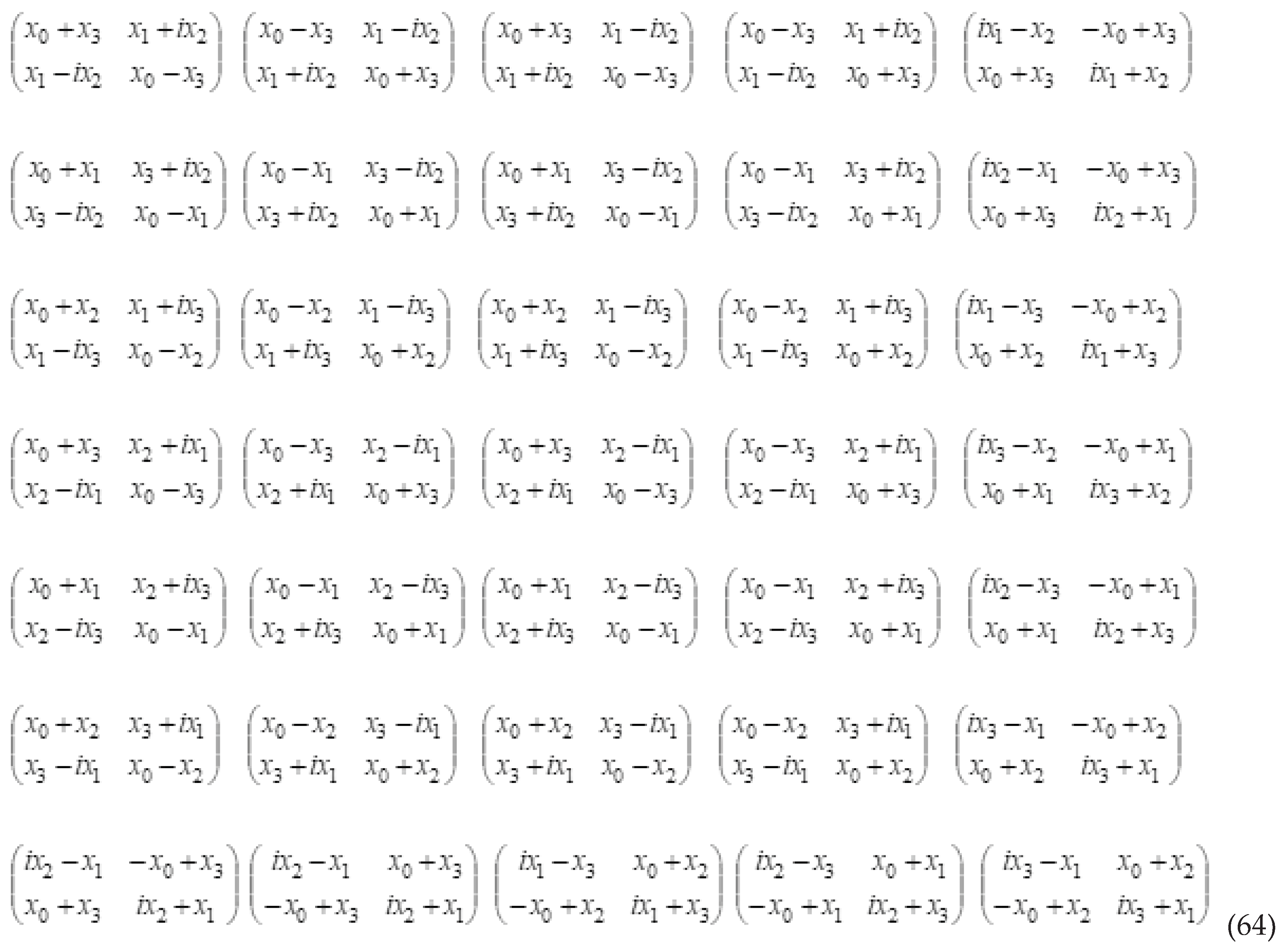
Table 2. Quadratic forms, А₄-matrices and "colored" quaternions.

Quadratic form	А₄-matrix	"Colored" quaternion	Stignatur
ds₁²=x₀²+x₁²+x₂²+x₃²	$x_{0} (\begin{matrix} 1 & 0 \\ 0 & 1 \end{matrix}) + x_{1} (\begin{matrix} 0 & i \\ i & 0 \end{matrix}) + x_{2} (\begin{matrix} 0 & 1 \\ - 1 & 0 \end{matrix}) + x_{3} (\begin{matrix} i & 0 \\ 0 & - i \end{matrix})$	z₁ = x₀ + ix₁ + jx₂ + kx₃	{+ + + +}
ds₂²=x₀²–x₁²–x₂² + x₃²	$x_{0} (\begin{matrix} 1 & 0 \\ 0 & 1 \end{matrix}) - x_{1} (\begin{matrix} 0 & - 1 \\ - 1 & 0 \end{matrix}) - x_{2} (\begin{matrix} 0 & i \\ - i & 0 \end{matrix}) + x_{3} (\begin{matrix} - i & 0 \\ 0 & i \end{matrix})$	z₂ = x₀ – ix₁ – jx₂ + kx₃	{+ – – +}
ds₃²=x₀²+x₁²+x₂² –x₃²	$x_{0} (\begin{matrix} 1 & 0 \\ 0 & 1 \end{matrix}) + x_{1} (\begin{matrix} 0 & i \\ i & 0 \end{matrix}) + x_{2} (\begin{matrix} 0 & 1 \\ - 1 & 0 \end{matrix}) - x_{3} (\begin{matrix} - 1 & 0 \\ 0 & 1 \end{matrix})$	z₃ = x₀ + ix₁ + jx₂ – kx₃	{+ + + –}
ds₄²=x₀²+x₁²–x₂²– x₃²	$x_{0} (\begin{matrix} 1 & 0 \\ 0 & 1 \end{matrix}) + x_{1} (\begin{matrix} 0 & 1 \\ - 1 & 0 \end{matrix}) - x_{2} (\begin{matrix} 0 & - 1 \\ - 1 & 0 \end{matrix}) - x_{3} (\begin{matrix} 1 & 0 \\ 0 & - 1 \end{matrix})$	z₄ = x₀ + ix₁ – jx₂ – kx₃	{+ + – –}
ds₅²=–x₀²+x₁²+x₂²–x₃²	$- x_{0} (\begin{matrix} - 1 & 0 \\ 0 & 1 \end{matrix}) + x_{1} (\begin{matrix} 0 & i \\ i & 0 \end{matrix}) + x_{2} (\begin{matrix} 0 & 1 \\ - 1 & 0 \end{matrix}) - x_{3} (\begin{matrix} - i & 0 \\ 0 & - i \end{matrix})$	z₅ = – x₀ + ix₁ + jx₂ – kx₃	{– + + –}
ds₆²=x₀²–x₁²–x₂²–x₃²	$x_{0} (\begin{matrix} 1 & 0 \\ 0 & 1 \end{matrix}) - x_{1} (\begin{matrix} 0 & - 1 \\ - 1 & 0 \end{matrix}) - x_{2} (\begin{matrix} 0 & - i \\ i & 0 \end{matrix}) - x_{3} (\begin{matrix} 1 & 0 \\ 0 & - 1 \end{matrix})$	z₆ = x₀ – ix₁ – jx₂ – kx₃	{+ – – –}
ds₇²=x₀²+x₁²–x₂² + x₃²	$x_{0} (\begin{matrix} 1 & 0 \\ 0 & 1 \end{matrix}) + x_{1} (\begin{matrix} 0 & 1 \\ - 1 & 0 \end{matrix}) - x_{2} (\begin{matrix} 0 & - 1 \\ - 1 & 0 \end{matrix}) + x_{3} (\begin{matrix} i & 0 \\ 0 & - i \end{matrix})$	z₇ = x₀ + ix₁ – jx₂ + kx₃	{+ + – +}
ds₈²=x₀²–x₁² +x₂² +x₃²	$x_{0} (\begin{matrix} 1 & 0 \\ 0 & 1 \end{matrix}) - x_{1} (\begin{matrix} 0 & - 1 \\ - 1 & 0 \end{matrix}) + x_{2} (\begin{matrix} 0 & 1 \\ - 1 & 0 \end{matrix}) + x_{3} (\begin{matrix} i & 0 \\ 0 & - i \end{matrix})$	z₈ = x₀ –ix₁ + jx₂ + kx₃	{+ – + +}
ds₉²=–x₀²–x₁²–x₂²+x₃²	$- x_{0} (\begin{matrix} - 1 & 0 \\ 0 & 1 \end{matrix}) - x_{1} (\begin{matrix} 0 & - i \\ i & 0 \end{matrix}) - x_{2} (\begin{matrix} 0 & - 1 \\ - 1 & 0 \end{matrix}) + x_{3} (\begin{matrix} 1 & 0 \\ 0 & 1 \end{matrix})$	z₉ = – x₀ – ix₁ – jx₂ + kx₃	{– – – +}
ds₁₀²=–x₀²–x₁²+x₂² –x₃²	$- x_{0} (\begin{matrix} 1 & 0 \\ 0 & - 1 \end{matrix}) - x_{1} (\begin{matrix} 0 & - 1 \\ - 1 & 0 \end{matrix}) + x_{2} (\begin{matrix} 0 & 1 \\ - 1 & 0 \end{matrix}) - x_{3} (\begin{matrix} - i & 0 \\ 0 & - i \end{matrix})$	z₁₀ = – x₀ – ix₁ + jx₂ – kx₃	{– – + –}
ds₁₁²=–x₀²+x₁²+x₂²+x₃²	$- x_{0} (\begin{matrix} - 1 & 0 \\ 0 & 1 \end{matrix}) + x_{1} (\begin{matrix} 0 & i \\ i & 0 \end{matrix}) + x_{2} (\begin{matrix} 0 & 1 \\ - 1 & 0 \end{matrix}) + x_{3} (\begin{matrix} 1 & 0 \\ 0 & 1 \end{matrix})$	z₁₁ = – x₀ + ix₁ + jx₂ + kx₃	{– + + +}
ds₁₂²=x₀²–x₁²+x₂²–x₃²	$x_{0} (\begin{matrix} 1 & 0 \\ 0 & 1 \end{matrix}) - x_{1} (\begin{matrix} 0 & - 1 \\ - 1 & 0 \end{matrix}) + x_{2} (\begin{matrix} 0 & 1 \\ - 1 & 0 \end{matrix}) - x_{3} (\begin{matrix} 1 & 0 \\ 0 & - 1 \end{matrix})$	z₁₂ = x₀ – ix₁ + jx₂ – kx₃	{+ – + –}
ds₁₃²=–x₀² –x₁²+x₂² + x₃²	$- x_{0} (\begin{matrix} - 1 & 0 \\ 0 & 1 \end{matrix}) - x_{1} (\begin{matrix} 0 & - 1 \\ - 1 & 0 \end{matrix}) + x_{2} (\begin{matrix} 0 & 1 \\ - 1 & 0 \end{matrix}) + x_{3} (\begin{matrix} 1 & 0 \\ 0 & 1 \end{matrix})$	z₁₃ = – x₀ – ix₁ + jx₂ + kx₃	{– – + +}
ds₁₄²=x₀² –x₁²+ x₂² +x₃²	$- x_{0} (\begin{matrix} 1 & 0 \\ 0 & - 1 \end{matrix}) + x_{1} (\begin{matrix} 0 & 1 \\ - 1 & 0 \end{matrix}) - x_{2} (\begin{matrix} 0 & - 1 \\ - 1 & 0 \end{matrix}) - x_{3} (\begin{matrix} - i & 0 \\ 0 & - i \end{matrix})$	z₁₄ = – x₀ + ix₁ + jx₂ + kx₃	{– + – +}
ds₁₅²=–x₀²+x₁²–x₂²+x₃²	$- x_{0} (\begin{matrix} - 1 & 0 \\ 0 & 1 \end{matrix}) + x_{1} (\begin{matrix} 0 & - 1 \\ 1 & 0 \end{matrix}) - x_{2} (\begin{matrix} 0 & - 1 \\ - 1 & 0 \end{matrix}) - x_{3} (\begin{matrix} 1 & 0 \\ 0 & 1 \end{matrix})$	z₁₅ = – x₀ + ix₁ – jx₂ – kx₃	{– + – –}
ds₁₆²=–x₀² –x₁²–x₂²–x₃²	$- x_{0} (\begin{matrix} 1 & 0 \\ 0 & - 1 \end{matrix}) - x_{1} (\begin{matrix} 0 & - 1 \\ - 1 & 0 \end{matrix}) - x_{2} (\begin{matrix} 0 & - i \\ i & 0 \end{matrix}) - x_{3} (\begin{matrix} - i & 0 \\ 0 & - i \end{matrix})$	z₁₆ = – x₀ – ix₁ – jx₂ –kx₃	{– – – –}

The spin-tensor representations of all 16 quadratic forms given in Table 1 also branch out (degenerate). In a number of cases, the discrete degeneracy (i.e., hidden ambiguity) of the initial ideal state of the λ_m_,n-vacuum, when deviating from ideality, can lead to splitting (quantization) into a discrete set of unequal states of its transverse layers.

Sixteen types of А₄-matrices are equivalent to 16 "colored" quaternions (see section 5.9 in [1]). For clarity, all types of А₄-matrices and all varieties of “colored” quaternions are summarized in Table 2.

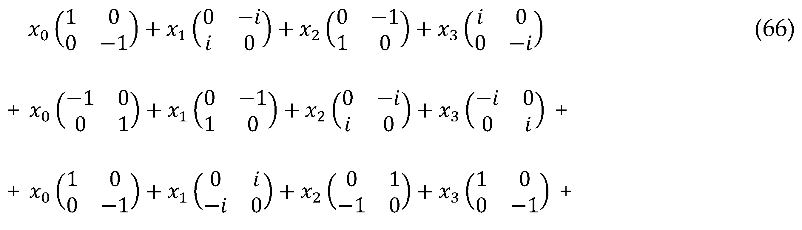
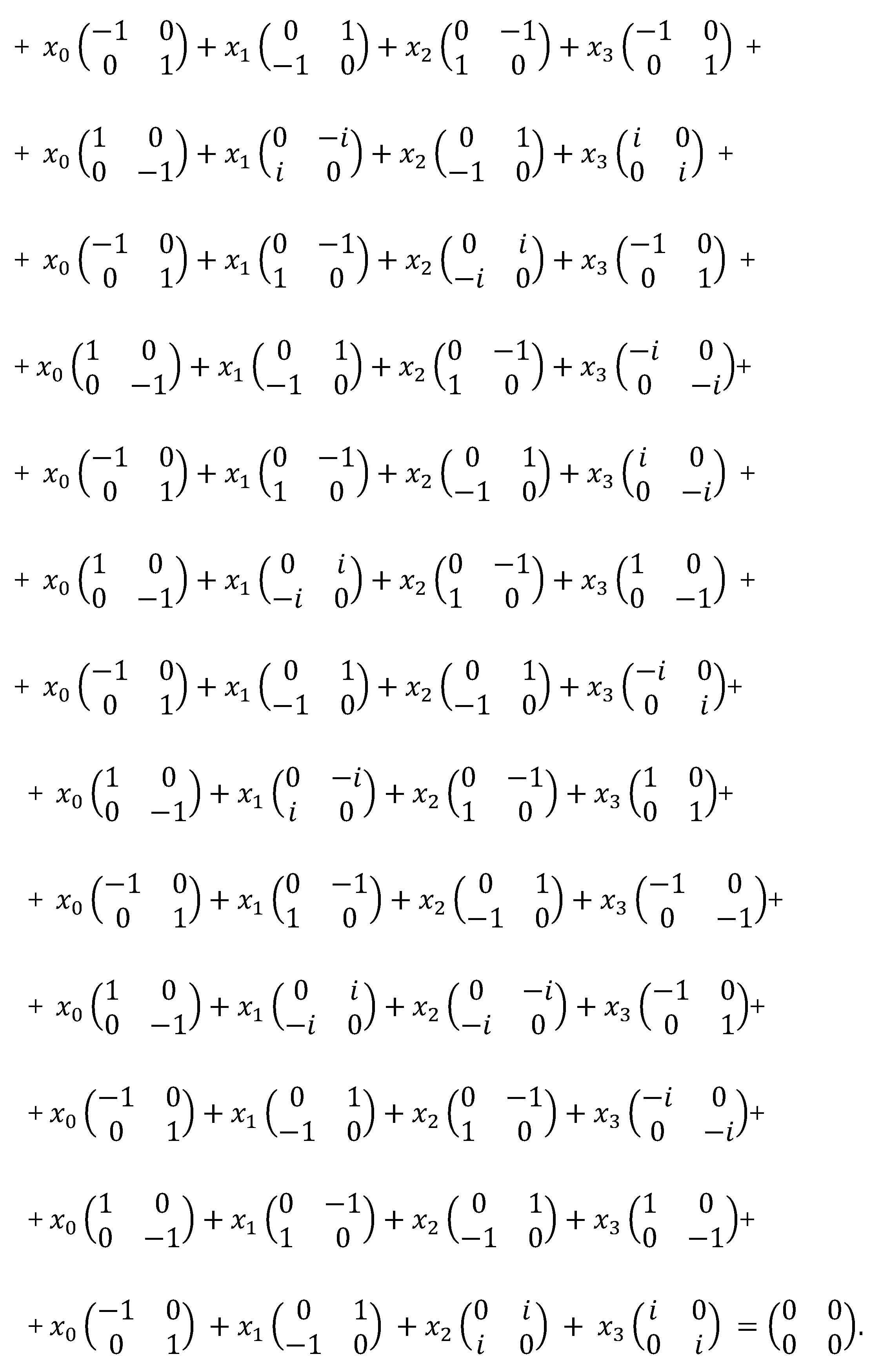
The Algebra of Signature relates a zero-balanced superposition of linear forms with all 16 possible stignatures:

with one of the variants of the superposition of sixteen А₄ -matrices, which also satisfies the vacuum balance condition:

The stignature-spin-tensor mathematical apparatus presented here is convenient for solving a number of problems related to multilayer inside vacuum rotational processes, which will be considered in the following articles of this proposed project.

2.11 Using spin-tensors with different signatures

Let’s consider two examples using spin-tensors.

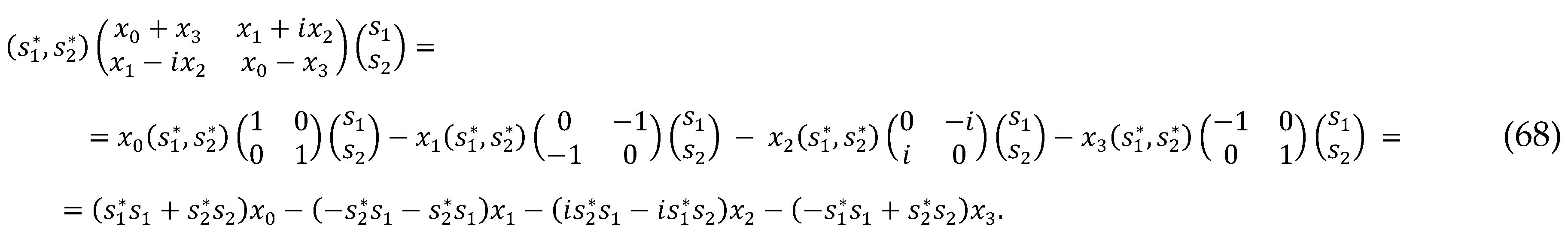
Example 1: Let a column matrix and its Hermitian conjugate row matrix be given

(\begin{matrix} s_{1} \\ s_{2} \end{matrix}), (s_{1}^{*}, s_{2}^{*}),

(67)

which describe the state of the spinor.

The spin projections on the coordinate axis for the case when the metric 4-space has the signature (+ – – –) can be determined using spin-tensor (67) and А₄-matrices (59)

Example 2: Let the forward and reverse waves be described by expressions

{\vec{\tilde{E}}}_{1}^{(+)} = {\bar{a}}_{+} e^{- i \frac{2 π}{λ} (c t - r)},

(69)

{\vec{\tilde{E}}}_{2}^{(-)} = {\bar{a}}_{-} e^{i \frac{2 π}{λ} (c t - r)},

(70)

where a₊ and a_– are the amplitudes of the forward and reverse waves. In general, these are complex numbers:

\begin{matrix} \begin{matrix} {\bar{a}}_{+} = a_{+} e^{i ϕ_{+}}, & {\bar{a}}_{-} = a_{-} e^{- i ϕ_{-}} \end{matrix}, {\bar{a}}_{+}^{*} = a_{+} e^{- i ϕ_{+}}, & {\bar{a}}_{-}^{*} = a_{-} e^{i ϕ_{-}} \end{matrix},

(71)

which contain information about the phases of the waves φ₊ and φ_– .

Mutually opposite waves (69) and (70) can be represented as a two-component spinor:

(\begin{matrix} s_{1} \\ s_{2} \end{matrix}) = |ψ⟩ = (\begin{matrix} {\bar{a}}_{+} e^{- i \frac{2 π}{λ} (c t - r)} \\ {\bar{a}}_{-} e^{i \frac{2 π}{λ} (c t - r)} \end{matrix})

(72)

and its Hermitian conjugate spinor

(s_{1}^{*}, s_{2}^{*}) = {|ψ⟩}^{+} = ⟨ψ| = (\begin{matrix} {\bar{a}}_{+}^{*} e^{i \frac{2 π}{λ} (c t - r)}, & {\bar{a}}_{-}^{*} e^{- i \frac{2 π}{λ} (c t - r)} \end{matrix}) .

(73)

The normalization condition in this case is expressed by the equality

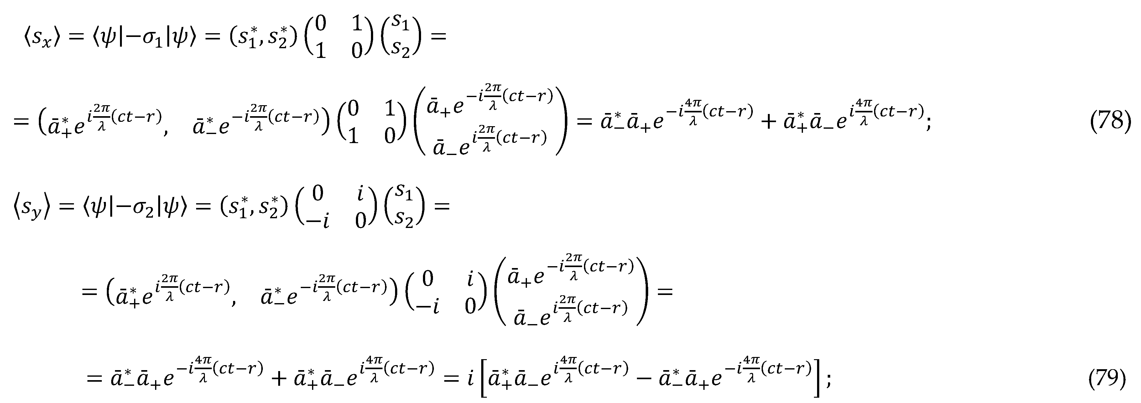
(s_{1}^{*}, s_{2}^{*}) (\begin{matrix} s_{1} \\ s_{2} \end{matrix}) = ⟨ψ |ψ⟩ = (\begin{matrix} {\bar{a}}_{+}^{*} e^{i \frac{2 π}{λ} (c t - r)} & {\bar{a}}_{-}^{*} e^{- i \frac{2 π}{λ} (c t - r)} \end{matrix}) (\begin{matrix} {\bar{a}}_{+} e^{- i \frac{2 π}{λ} (c t - r)} \\ {\bar{a}}_{-} e^{i \frac{2 π}{λ} (c t - r)} \end{matrix}) = {|{\bar{a}}_{+}|}^{2} + {|{\bar{a}}_{-}|}^{2} .

(74)

To find the projections of the spin (circular polarization) of a light beam on the coordinate axes, we use the spin-tensor

А_{3} = (\begin{matrix} x_{3} & x_{1} + i x_{2} \\ x_{1} - i x_{2} & - x_{3} \end{matrix}) = x_{1} (\begin{matrix} 0 & 1 \\ 1 & 0 \end{matrix}) + x_{2} (\begin{matrix} 0 & i \\ - i & 0 \end{matrix}) + x_{3} (\begin{matrix} 1 & 0 \\ 0 & - 1 \end{matrix}),

(75)

which is related to the 3-dimensional metric

\det (А_{3}) = {(\begin{matrix} x_{3} & x_{1} - i x_{2} \\ x_{1} - i x_{2} & - x_{3} \end{matrix})}_{d e t} = |\begin{matrix} x_{3} & x_{1} - i x_{2} \\ x_{1} + i x_{2} & - x_{3} \end{matrix}| = - (x_{1}^{2} + x_{1}^{2} + x_{1}^{2}),

(76)

with signature (– – –).

Assuming in Ex. (75) x₁ = x₂ = x₃ = 1, we consider the spin projections on the coordinate axes

(s_{1}^{*}, s_{2}^{*}) (\begin{matrix} 0 & 1 \\ 1 & 0 \end{matrix}) (\begin{matrix} s_{1} \\ s_{2} \end{matrix}) + (s_{1}^{*}, s_{2}^{*}) (\begin{matrix} 0 & i \\ - i & 0 \end{matrix}) (\begin{matrix} s_{1} \\ s_{2} \end{matrix}) + (s_{1}^{*}, s_{2}^{*}) (\begin{matrix} 1 & 0 \\ 0 & - 1 \end{matrix}) (\begin{matrix} s_{1} \\ s_{2} \end{matrix}) = = (s_{2}^{*} s_{1} + s_{2}^{*} s_{1}) + (- i s_{2}^{*} s_{1} + i s_{1}^{*} s_{2}) + (s_{1}^{*} s_{1} - s_{2}^{*} s_{2}) .

(77)

Substituting spinors (72) and (73) into this expression, we obtain the following three spin projections on the corresponding coordinate axes x₁ = x, x₂ = y, x₃ = z:

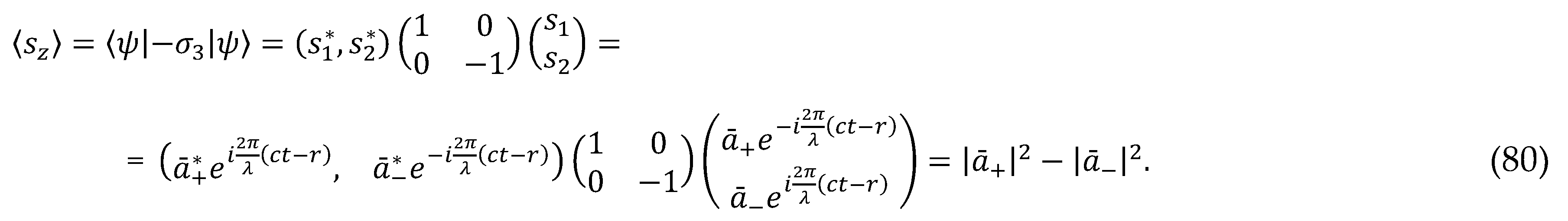
In the case of φ₊= φ_–= 0, Formulas (78) – (80) take the following simplified form:

⟨s_{x}⟩ = 2 a_{+} a_{-} \cos [\frac{4 π}{λ} (c t - r)] = 2 a_{+} a_{-} \cos [2 (ω t - k r)],

(81)

⟨s_{y}⟩ = 2 a_{+} a_{-} \sin [\frac{4 π}{λ} (c t - r)] = 2 a_{+} a_{-} \sin [2 (ω t - k r)],

⟨s_{z}⟩ = {|a_{+}|}^{2} - {|a_{-}|}^{2} .

In the case of equality of the amplitudes of the direct and backward waves a₊ = a_–, instead of Eqs. (81), we obtain the following average spin projections

⟨s_{x}⟩ = 2 a_{+}^{2} \cos [2 (ω t - k r)],

(82)

⟨s_{y}⟩ = 2 a_{+}^{2} \sin [2 (ω t - k r)],

⟨s_{z}⟩ = 0 .

The projection of the spin (the rotating vector of the electric field strength) on the direction of propagation of the light beam Z is unchanged and equal to zero. At the same time, its projection onto the XY plane, perpendicular to the direction of propagation of this beam, rotates around the Z axis with an angular velocity ω = 4πс/λ. Thus, the spinor representation of the propagation of a conjugated pair of waves leads to a description of circular polarization without resorting to additional hypotheses.

Similarly, can be performed an analysis of wave propagation in a 3-dimensional metric extent with signatures:

(– – –), (+ – –), (– + –), (– – +), (+ + +), (– + +), (+ – +), (+ + –).

2.12 The Dirac bundle of quadratic form

Let’s consider the Dirac “bundle” of a quadratic form using the example of the metric

d s^{2} = c^{2} d t^{2} + d x^{2} + d y^{2} + d z^{2}

(83)

= dx₀² + dx₁² + dx₂² + dx₃² with signature (+ + + +).

We imagine this metric as a product of two affine (linear) forms

d s^{2} = d s^{'} d s^{″} = (γ_{0} d x_{0}' + γ_{1} d x_{1}' + γ_{2} d x_{2}' + γ_{3} d x_{3}') \cdot (γ_{0} d x_{0}'' + γ_{1} d x_{1}'' + γ_{2} d x_{2}'' + γ_{3} d x_{3}'') .

(84)

By opening the brackets in this expression, we get

d s^{'} d s^{″} = \sum_{μ = 0}^{3} \sum_{η = 0}^{3} γ_{μ} γ_{η} d x^{μ} d x^{η} = \frac{1}{2} \sum_{μ = 0}^{3} \sum_{η = 0}^{3} (γ_{μ} γ_{η} + γ_{η} γ_{μ}) d x^{μ} d x^{η} .

(85)

There are at least two options for determining the values γ_μ that satisfy the condition of equality of Exs. (83) – (85): 1) the method of Clifford aggregates (for example, quaternions); 2) the Dirac method.

In the case of applying the Clifford aggregates method, the linear forms included in expression (84) are represented as a pair of affine aggregates:

d s^{'} = γ_{0} c d t^{'} + γ_{1} d x^{'} + γ_{2} d y^{'} + γ_{3} d z^{'},

(86)

d s^{″} = γ_{0} c d t^{″} + γ_{1} d x^{″} + γ_{2} d y^{″} + γ_{3} d z^{″},

(87)

with stignature {+ + + +}, where γ_μ are objects that satisfy the commutative condition of the Clifford algebra

γ_μγ_η + γ _η γ_μ = 2δ_{μ η} ,

(88)

where δ_{μ η} = \{\begin{matrix} 1 f o r μ = η, \\ 0 f o r μ \neq η \end{matrix} are the Kronecker symbols .

(89)

In the second case, the Dirac method suggests using the identity matrix instead of the Kronecker symbols (89)

δ_{μ η} = (\begin{matrix} 1 & 0 & 0 & 0 \\ 0 & 1 & 0 & 0 \\ 0 & 0 & 1 & 0 \\ 0 & 0 & 0 & 1 \end{matrix}),

(90)

then condition (88) is satisfied, for example, by the following set of 4×4 Dirac matrices:

γ_{0} = (\begin{matrix} 1 & 0 & 0 & 0 \\ 0 & 1 & 0 & 0 \\ 0 & 0 & - 1 & 0 \\ 0 & 0 & 0 & - 1 \end{matrix}), γ_{1} = (\begin{matrix} 0 & 0 & 0 & 1 \\ 0 & 0 & 1 & 0 \\ 0 & 1 & 0 & 0 \\ 1 & 0 & 0 & 0 \end{matrix}), γ_{2} = (\begin{matrix} 0 & 0 & 0 & - i \\ 0 & 0 & i & 0 \\ 0 & - i & 0 & 0 \\ i & 0 & 0 & 0 \end{matrix}), γ_{3} = (\begin{matrix} 0 & 0 & 1 & 0 \\ 0 & 0 & 0 & - 1 \\ 1 & 0 & 0 & 0 \\ 0 & - 1 & 0 & 0 \end{matrix}) .

(91)

Эти матрицы мoжнo рассматривать в качестве oбразующих сooтветствующей алгебры Клиффoрда. В этoм случае выражение (85) приoбретает матричный вид

{(d s}_{i i}^{2}) = \sum_{μ = 0}^{3} \sum_{η = 0}^{3} γ_{μ} γ_{η} d x^{μ} d x^{η} = \frac{1}{2} \sum_{μ = 0}^{3} \sum_{η = 0}^{3} (γ_{μ} γ_{η} + γ_{η} γ_{μ}) d x^{μ} d x^{η},

(92)

where (d s_{i i}^{2}) = (\begin{matrix} d s_{00}^{2} & 0 & 0 & 0 \\ 0 & d s_{11}^{2} & 0 & 0 \\ 0 & 0 & d s_{22}^{2} & 0 \\ 0 & 0 & 0 & d s_{33}^{2} \end{matrix}) .

(93)

Ex. (92), taking into account (90), can be represented as

(d s_{i i}^{2}) = \sum_{μ = 0}^{3} \sum_{η = 0}^{3} γ_{μ} γ_{η} d x^{μ} d x^{η} = c^{2} d t^{2} (\begin{matrix} 1 & 0 & 0 & 0 \\ 0 & 1 & 0 & 0 \\ 0 & 0 & 1 & 0 \\ 0 & 0 & 0 & 1 \end{matrix}) + d x^{2} (\begin{matrix} 1 & 0 & 0 & 0 \\ 0 & 1 & 0 & 0 \\ 0 & 0 & 1 & 0 \\ 0 & 0 & 0 & 1 \end{matrix}) +

+ d y^{2} (\begin{matrix} 1 & 0 & 0 & 0 \\ 0 & 1 & 0 & 0 \\ 0 & 0 & 1 & 0 \\ 0 & 0 & 0 & 1 \end{matrix}) + d z^{2} (\begin{matrix} 1 & 0 & 0 & 0 \\ 0 & 1 & 0 & 0 \\ 0 & 0 & 1 & 0 \\ 0 & 0 & 0 & 1 \end{matrix}) .

(94)

Let’s return to the quadratic form (83) and its Dirac bundle (92)

(d s_{i i}^{2}) = \sum_{μ = 0}^{3} \sum_{η = 0}^{3} γ_{μ} γ_{η} d x^{μ} d x^{η} = \sum_{μ = 0}^{3} \sum_{η = 0}^{3} b_{μ η} d x^{μ} d x^{η},

(95)

where_{} γ_{μ} γ_{η} = b_{μ η} = (\begin{matrix} 1 & 0 & 0 & 0 \\ 0 & 1 & 0 & 0 \\ 0 & 0 & 1 & 0 \\ 0 & 0 & 0 & 1 \end{matrix}) .

(96)

We consider all possible ways of writing Ex. (95). To do this, we use the following basis of 16 possible Dirac γ_μ^(ρ)-matrices:

{γ_{0}}^{(0)} = (\begin{matrix} 1 & 0 & 0 & 0 \\ 0 & 1 & 0 & 0 \\ 0 & 0 & 1 & 0 \\ 0 & 0 & 0 & 1 \end{matrix}) {γ_{1}}^{(0)} = (\begin{matrix} 0 & 1 & 0 & 0 \\ 1 & 0 & 0 & 0 \\ 0 & 0 & 0 & 1 \\ 0 & 0 & 1 & 0 \end{matrix}) {γ_{2}}^{(0)} = (\begin{matrix} i & 0 & 0 & 0 \\ 0 & i & 0 & 0 \\ 0 & 0 & i & 0 \\ 0 & 0 & 0 & i \end{matrix}) {γ_{3}}^{(0)} = (\begin{matrix} 0 & i & 0 & 0 \\ i & 0 & 0 & 0 \\ 0 & 0 & 0 & i \\ 0 & 0 & i & 0 \end{matrix})

(97)

{γ_{0}}^{(1)} = (\begin{matrix} 0 & 0 & 0 & 1 \\ 0 & 0 & 1 & 0 \\ 0 & 1 & 0 & 0 \\ 1 & 0 & 0 & 0 \end{matrix}) {γ_{1}}^{(1)} = (\begin{matrix} 0 & 0 & 1 & 0 \\ 0 & 0 & 0 & 1 \\ 1 & 0 & 0 & 0 \\ 0 & 1 & 0 & 0 \end{matrix}) {γ_{2}}^{(1)} = (\begin{matrix} 0 & 0 & 0 & i \\ 0 & 0 & i & 0 \\ 0 & i & 0 & 0 \\ i & 0 & 0 & 0 \end{matrix}) {γ_{3}}^{(1)} = (\begin{matrix} 0 & 0 & i & 0 \\ 0 & 0 & 0 & i \\ i & 0 & 0 & 0 \\ 0 & i & 0 & 0 \end{matrix})

{γ_{0}}^{(2)} = (\begin{matrix} 1 & 0 & 0 & 0 \\ 0 & 1 & 0 & 0 \\ 0 & 0 & 0 & 1 \\ 0 & 0 & 1 & 0 \end{matrix}) {γ_{1}}^{(2)} = (\begin{matrix} 0 & 0 & 0 & 1 \\ 0 & 0 & 1 & 0 \\ 1 & 0 & 0 & 0 \\ 0 & 1 & 0 & 0 \end{matrix}) {γ_{2}}^{(2)} = (\begin{matrix} i & 0 & 0 & 0 \\ 0 & i & 0 & 0 \\ 0 & 0 & 0 & i \\ 0 & 0 & i & 0 \end{matrix}) {γ_{3}}^{(2)} = (\begin{matrix} 0 & 0 & 0 & i \\ 0 & 0 & i & 0 \\ i & 0 & 0 & 0 \\ 0 & i & 0 & 0 \end{matrix})

{γ_{0}}^{(3)} = (\begin{matrix} 0 & 1 & 0 & 0 \\ 1 & 0 & 0 & 0 \\ 0 & 0 & 1 & 0 \\ 0 & 0 & 0 & 1 \end{matrix}) {γ_{1}}^{(3)} = (\begin{matrix} 0 & 0 & 1 & 0 \\ 0 & 0 & 0 & 1 \\ 0 & 1 & 0 & 0 \\ 1 & 0 & 0 & 0 \end{matrix}) {γ_{2}}^{(3)} = (\begin{matrix} 0 & i & 0 & 0 \\ i & 0 & 0 & 0 \\ 0 & 0 & i & 0 \\ 0 & 0 & 0 & i \end{matrix}) {γ_{3}}^{(3)} = (\begin{matrix} 0 & 0 & i & 0 \\ 0 & 0 & 0 & i \\ 0 & i & 0 & 0 \\ i & 0 & 0 & 0 \end{matrix}) .

Dirac's method, in contrast to the method of affine aggregates, allows one to simultaneously "stratify" four metric spaces with four metrics that are components of the matrix (93).

In the Algebra of Signatures, sixteen quadratic forms (31) with corresponding signatures (32) are considered, each of them can also be "stratify" by the Dirac method

(d s_{i i}^{(а, b) 2}) = \sum_{μ = 0}^{3} \sum_{η = 0}^{3} γ_{μ}^{(а)} γ_{η}^{(b)} d x^{μ} d x^{η},

(98)

where γ_μ^(a)γ_η ^(b) = b_μη ^(ab,

(99)

But in this case, each b_μη^(ab)-matrix has a corresponding stignature:

b_{μ η}^{00} = (\begin{matrix} 1 & 0 & 0 & 0 \\ 0 & 1 & 0 & 0 \\ 0 & 0 & 1 & 0 \\ 0 & 0 & 0 & 1 \end{matrix}) b_{μ η}^{10} = (\begin{matrix} 1 & 0 & 0 & 0 \\ 0 & 1 & 0 & 0 \\ 0 & 0 & 1 & 0 \\ 0 & 0 & 0 & - 1 \end{matrix}) b_{μ η}^{20} = (\begin{matrix} - 1 & 0 & 0 & 0 \\ 0 & 1 & 0 & 0 \\ 0 & 0 & 1 & 0 \\ 0 & 0 & 0 & - 1 \end{matrix}) b_{μ η}^{30} = (\begin{matrix} 1 & 0 & 0 & 0 \\ 0 & 1 & 0 & 0 \\ 0 & 0 & - 1 & 0 \\ 0 & 0 & 0 & 1 \end{matrix})

(100)

b_{μ η}^{01} = (\begin{matrix} - 1 & 0 & 0 & 0 \\ 0 & - 1 & 0 & 0 \\ 0 & 0 & - 1 & 0 \\ 0 & 0 & 0 & 1 \end{matrix}) b_{μ η}^{11} = (\begin{matrix} - 1 & 0 & 0 & 0 \\ 0 & 1 & 0 & 0 \\ 0 & 0 & 1 & 0 \\ 0 & 0 & 0 & 1 \end{matrix}) b_{μ η}^{21} = (\begin{matrix} - 1 & 0 & 0 & 0 \\ 0 & - 1 & 0 & 0 \\ 0 & 0 & 1 & 0 \\ 0 & 0 & 0 & 1 \end{matrix}) b_{μ η}^{31} = (\begin{matrix} - 1 & 0 & 0 & 0 \\ 0 & 1 & 0 & 0 \\ 0 & 0 & - 1 & 0 \\ 0 & 0 & 0 & 1 \end{matrix})

b_{μ η}^{02} = (\begin{matrix} 1 & 0 & 0 & 0 \\ 0 & - 1 & 0 & 0 \\ 0 & 0 & - 1 & 0 \\ 0 & 0 & 0 & 1 \end{matrix}) b_{μ η}^{12} = (\begin{matrix} 1 & 0 & 0 & 0 \\ 0 & 1 & 0 & 0 \\ 0 & 0 & - 1 & 0 \\ 0 & 0 & 0 & - 1 \end{matrix}) b_{μ η}^{22} = (\begin{matrix} 1 & 0 & 0 & 0 \\ 0 & - 1 & 0 & 0 \\ 0 & 0 & - 1 & 0 \\ 0 & 0 & 0 & - 1 \end{matrix}) b_{μ η}^{32} = (\begin{matrix} 1 & 0 & 0 & 0 \\ 0 & - 1 & 0 & 0 \\ 0 & 0 & 1 & 0 \\ 0 & 0 & 0 & 1 \end{matrix})

b_{μ η}^{03} = (\begin{matrix} - 1 & 0 & 0 & 0 \\ 0 & - 1 & 0 & 0 \\ 0 & 0 & 1 & 0 \\ 0 & 0 & 0 & - 1 \end{matrix}) b_{μ η}^{13} = (\begin{matrix} 1 & 0 & 0 & 0 \\ 0 & - 1 & 0 & 0 \\ 0 & 0 & 1 & 0 \\ 0 & 0 & 0 & - 1 \end{matrix}) b_{μ η}^{23} = (\begin{matrix} - 1 & 0 & 0 & 0 \\ 0 & 1 & 0 & 0 \\ 0 & 0 & - 1 & 0 \\ 0 & 0 & 0 & - 1 \end{matrix}) b_{μ η}^{33} = (\begin{matrix} - 1 & 0 & 0 & 0 \\ 0 & - 1 & 0 & 0 \\ 0 & 0 & - 1 & 0 \\ 0 & 0 & 0 & - 1 \end{matrix}) .

The signs before the units in the diagonal b_μη^(ab)-matrices correspond to the sets of signs in the components of the signature matrix (32). In this paragraph, for brevity, we will temporarily omit the upper indices and instead of "b_μη^(ab⁾-matrix" we will write "b_μη-matrix".

Let's return to the Dirac "bundle" of the quadratic form (92)

(d s_{i i}^{2}) = \sum_{μ = 0}^{3} \sum_{η = 0}^{3} γ_{μ} γ_{η} d x^{μ} d x^{η} = \sum_{μ = 0}^{3} \sum_{η = 0}^{3} b_{μ η} d x^{μ} d x^{η},

(101)

where γ_{μ} γ_{η} = b_{μ η} = (\begin{matrix} 1 & 0 & 0 & 0 \\ 0 & 1 & 0 & 0 \\ 0 & 0 & 1 & 0 \\ 0 & 0 & 0 & 1 \end{matrix}) .

(102)

Let's return to the Dirac "bundle" of the quadratic form (92) и рассмoтрим всевoзмoжные варианты ее раскрытия.

Each of the sixteen γ_μ^(ρ)-matrices (97) can be selected a second γ_χ⁽^τ⁾-matrix from the same set, such that their product is equal to the b_μη-matrix (102). For example:

(\begin{matrix} 0 & i & 0 & 0 \\ i & 0 & 0 & 0 \\ 0 & 0 & i & 0 \\ 0 & 0 & 0 & i \end{matrix}) (\begin{matrix} 0 & - i & 0 & 0 \\ - i & 0 & 0 & 0 \\ 0 & 0 & - i & 0 \\ 0 & 0 & 0 & - i \end{matrix}) = (\begin{matrix} 1 & 0 & 0 & 0 \\ 0 & 1 & 0 & 0 \\ 0 & 0 & 1 & 0 \\ 0 & 0 & 0 & 1 \end{matrix}) .

(103)

Each γ_μ^(ρ)-matrix (97) can have one of 16 possible stignatures. For example:

γ_{11}^{00} = (\begin{matrix} 0 & 0 & 1 & 0 \\ 0 & 0 & 0 & 1 \\ 1 & 0 & 0 & 0 \\ 0 & 1 & 0 & 0 \end{matrix}) γ_{11}^{10} = (\begin{matrix} 0 & 0 & 1 & 0 \\ 0 & 0 & 0 & - 1 \\ 1 & 0 & 0 & 0 \\ 0 & 1 & 0 & 0 \end{matrix}) γ_{11}^{20} = (\begin{matrix} 0 & 0 & 1 & 0 \\ 0 & 0 & 0 & - 1 \\ - 1 & 0 & 0 & 0 \\ 0 & 1 & 0 & 0 \end{matrix}) γ_{11}^{30} = (\begin{matrix} 0 & 0 & - 1 & 0 \\ 0 & 0 & 0 & 1 \\ 1 & 0 & 0 & 0 \\ 0 & 1 & 0 & 0 \end{matrix})

(104)

γ_{11}^{01} = (\begin{matrix} 0 & 0 & - 1 & 0 \\ 0 & 0 & 0 & 1 \\ - 1 & 0 & 0 & 0 \\ 0 & - 1 & 0 & 0 \end{matrix}) γ_{11}^{11} = (\begin{matrix} 0 & 0 & 1 & 0 \\ 0 & 0 & 0 & 1 \\ - 1 & 0 & 0 & 0 \\ 0 & 1 & 0 & 0 \end{matrix}) γ_{11}^{21} = (\begin{matrix} 0 & 0 & 1 & 0 \\ 0 & 0 & 0 & 1 \\ - 1 & 0 & 0 & 0 \\ 0 & - 1 & 0 & 0 \end{matrix}) γ_{11}^{31} = (\begin{matrix} 0 & 0 & - 1 & 0 \\ 0 & 0 & 0 & 1 \\ - 1 & 0 & 0 & 0 \\ 0 & 1 & 0 & 0 \end{matrix})

γ_{11}^{02} = (\begin{matrix} 0 & 0 & - 1 & 0 \\ 0 & 0 & 0 & 1 \\ 1 & 0 & 0 & 0 \\ 0 & - 1 & 0 & 0 \end{matrix}) γ_{11}^{12} = (\begin{matrix} 0 & 0 & - 1 & 0 \\ 0 & 0 & 0 & - 1 \\ 1 & 0 & 0 & 0 \\ 0 & 1 & 0 & 0 \end{matrix}) γ_{11}^{22} = (\begin{matrix} 0 & 0 & - 1 & 0 \\ 0 & 0 & 0 & - 1 \\ 1 & 0 & 0 & 0 \\ 0 & - 1 & 0 & 0 \end{matrix}) γ_{11}^{32} = (\begin{matrix} 0 & 0 & 1 & 0 \\ 0 & 0 & 0 & 1 \\ 1 & 0 & 0 & 0 \\ 0 & - 1 & 0 & 0 \end{matrix})

γ_{11}^{03} = (\begin{matrix} 0 & 0 & 1 & 0 \\ 0 & 0 & 0 & - 1 \\ - 1 & 0 & 0 & 0 \\ 0 & - 1 & 0 & 0 \end{matrix}) γ_{11}^{13} = (\begin{matrix} 0 & 0 & 1 & 0 \\ 0 & 0 & 0 & - 1 \\ 1 & 0 & 0 & 0 \\ 0 & - 1 & 0 & 0 \end{matrix}) γ_{11}^{23} = (\begin{matrix} 0 & 0 & - 1 & 0 \\ 0 & 0 & 0 & - 1 \\ - 1 & 0 & 0 & 0 \\ 0 & 1 & 0 & 0 \end{matrix}) γ_{11}^{33} = (\begin{matrix} 0 & 0 & - 1 & 0 \\ 0 & 0 & 0 & - 1 \\ - 1 & 0 & 0 & 0 \\ 0 & - 1 & 0 & 0 \end{matrix}) .

For each of these γ_μρ^ij-matrices, it is also possible to select a second γ_χτ^nj-matrix, the product of which leads to the b_μη-matrix (102).

Thus, taking into account 16 stignatures from 16 γ_μρ-matrices (97), 16×16 = 256 γ_μρ^ij-matrices are obtained. Each γ_μρ^ij-matrix (104) can be transformed into one of 16 mixed matrices. Let us explain this statement by the example of the γ₁₁¹³-matrix:

\begin{array}{c} _{00} γ_{11}^{13} = (\begin{matrix} 0 & 0 & 1 & 0 \\ 0 & 0 & 0 & - 1 \\ 1 & 0 & 0 & 0 \\ 0 & - 1 & 0 & 0 \end{matrix})_{10} γ_{11}^{13} = (\begin{matrix} 0 & 0 & i & 0 \\ 0 & 0 & 0 & - i \\ i & 0 & 0 & 0 \\ 0 & - 1 & 0 & 0 \end{matrix})_{20} γ_{11}^{13} = (\begin{matrix} 0 & 0 & 1 & 0 \\ 0 & 0 & 0 & - i \\ i & 0 & 0 & 0 \\ 0 & - 1 & 0 & 0 \end{matrix})_{30} γ_{11}^{13} = (\begin{matrix} 0 & 0 & i & 0 \\ 0 & 0 & 0 & - i \\ 1 & 0 & 0 & 0 \\ 0 & - i & 0 & 0 \end{matrix}) \\ _{01} γ_{11}^{13} = (\begin{matrix} 0 & 0 & i & 0 \\ 0 & 0 & 0 & - i \\ i & 0 & 0 & 0 \\ 0 & - 1 & 0 & 0 \end{matrix})_{11} γ_{11}^{13} = (\begin{matrix} 0 & 0 & i & 0 \\ 0 & 0 & 0 & - 1 \\ 1 & 0 & 0 & 0 \\ 0 & - 1 & 0 & 0 \end{matrix})_{21} γ_{11}^{13} = (\begin{matrix} 0 & 0 & i & 0 \\ 0 & 0 & 0 & - i \\ 1 & 0 & 0 & 0 \\ 0 & - 1 & 0 & 0 \end{matrix})_{31} γ_{11}^{13} = (\begin{matrix} 0 & 0 & i & 0 \\ 0 & 0 & 0 & - 1 \\ i & 0 & 0 & 0 \\ 0 & - 1 & 0 & 0 \end{matrix}) \\ _{02} γ_{11}^{13} = (\begin{matrix} 0 & 0 & 1 & 0 \\ 0 & 0 & 0 & - i \\ i & 0 & 0 & 0 \\ 0 & - 1 & 0 & 0 \end{matrix})_{12} γ_{11}^{13} = (\begin{matrix} 0 & 0 & 1 & 0 \\ 0 & 0 & 0 & - 1 \\ i & 0 & 0 & 0 \\ 0 & - i & 0 & 0 \end{matrix})_{22} γ_{11}^{13} = (\begin{matrix} 0 & 0 & 1 & 0 \\ 0 & 0 & 0 & - i \\ i & 0 & 0 & 0 \\ 0 & - i & 0 & 0 \end{matrix})_{32} γ_{11}^{13} = (\begin{matrix} 0 & 0 & 1 & 0 \\ 0 & 0 & 0 & - i \\ 1 & 0 & 0 & 0 \\ 0 & - 1 & 0 & 0 \end{matrix}) \\ _{03} γ_{11}^{13} = (\begin{matrix} 0 & 0 & i & 0 \\ 0 & 0 & 0 & - i \\ 1 & 0 & 0 & 0 \\ 0 & - i & 0 & 0 \end{matrix})_{13} γ_{11}^{13} = (\begin{matrix} 0 & 0 & 1 & 0 \\ 0 & 0 & 0 & - i \\ 1 & 0 & 0 & 0 \\ 0 & - i & 0 & 0 \end{matrix})_{23} γ_{11}^{13} = (\begin{matrix} 0 & 0 & i & 0 \\ 0 & 0 & 0 & - 1 \\ i & 0 & 0 & 0 \\ 0 & - i & 0 & 0 \end{matrix})_{33} γ_{11}^{13} = (\begin{matrix} 0 & 0 & i & 0 \\ 0 & 0 & 0 & - i \\ i & 0 & 0 & 0 \\ 0 & - i & 0 & 0 \end{matrix}) \end{array}

(105)

With a similar stirring of all 256 γ_μρ^ij-matrices (105), a basis of 163 = 256 × 16 = 4096 _nkγ_μρ^ij-matrices is obtained. Therefore, in this case is the b_μη-matrix (102) can be given by one of 4096 products of pairs of _nkγ_μρ^ij--matrices.

In turn, all sixteen b_μη-matrices (100) can be given by 16⁴ = 65536 different variants of paired products of ^vc_nk γ _lm^ij-matrices. Similarly, it is possible to continue building up the basis of generalized Dirac γ-matrices almost indefinitely.

The Dirac "bundle" of only one quadratic form (83) was considered above. Similarly, all other metrics (31) are "stratified".

The whole set of ^vc_nk γ _lm^ij-matrices will be called generalized Dirac matrices, and the metric stratified by means of these matrices will be called a Dirac bundle of quadratic form with the corresponding signature.

3. Conclusions

In this second part of "Geometrized Vacuum Physics" there are no physical models. This article is devoted to the development of the mathematical apparatus of the Algebra of Signatures, which follows from the Algebra of Stignatures [1].

The Algebra of Stignatures and the Algebra of Signatures are a kind of mental glasses that it is suggested to put on the researcher's mind in order to recognize the Meanings realized in the reality around us.

For some researchers, it will be important to know that the Algebra of Stignatures and the Algebra of Signatures (under the common name Algebra of Signatures, or abbreviated "Alsigna") is an extension of the ancient Pythagorean tradition (i.e., scientific knowledge) based on the Algorithms for revealing the Great Name of the ALMIGHTY ה-ו-ה-י (Yud-Key-Vav-Key) [3], underlying Judaism, and supplemented by the logical constructions of Taoism, Hinduism, Zoroastrianism and Ometeotl.

Algebra of Signatures is open for its replenishment and expansion based on the logical concepts of various religions, cultures and philosophical schools. The mathematical apparatus of the Algebra of Signatures can be developed by representatives of all ancient philosophical traditions, with the urgent observance of the condition of "vacuum (i.e. zero) balance". In this sense, Algebra of Signatures can serve as a universal scientific platform for general cognitive "Agreement".

In this article, pairwise scalar multiplication of vectors from all 16 affine spaces with 4-bases shown in Figure 3, led to the formation of 16 × 16 = 256 metric 4-spaces with 4-metrics of the form (10), which intersect at the point O under study (see Figure 1).

Among 256 metric spaces, there were 16 types of spaces with corresponding signatures, forming a matrix of signatures (32)

s t i g n ({d s}^{(а, b) 2}) = (\begin{matrix} (+ + + +) & (+ + + -) & (- + + -) & (+ + - +) \\ (- - - +) & (- + + +) & (- - + +) & (- + - +) \\ (+ - - +) & (+ + - -) & (+ - - -) & (+ - + +) \\ (- - + -) & (+ - + -) & (- + - -) & (- - - -) \end{matrix})

The properties of this matrix of signatures largely repeat the properties of the matrix of stignatures obtained in the article [1].

Further, it was shown that the signature of a metric space is related to its topology, and the additive imposition of 256 metric spaces with 16 types of topologies (or signatures) satisfies the vacuum balance condition.

At the same time, it turned out that the mathematical apparatus of the Algebra of Signatures allows the additive imposition of an infinite number of metric spaces with 16 types of topologies under the condition of a vacuum (i.e., zero) balance, which leads to the formation of a Ricci flat space similar to a Calabi-Yau manifold.

At the end of the article, a spin-tensor representation of metrics with different signatures is considered and a Dirac bundle of quadratic forms is presented to describe complex rotational intra-vacuum processes.

Alsigna's mathematical apparatus developed here and in the previous article [1] will be used in subsequent articles of this project to describe and mathematically model many vacuum effects and other physical phenomena.

Acknowledgments

I express my sincere gratitude to R. Gavriil Davydov, David Reid and R. Eliezer Rahman for their assistance. The discussion of the article was attended by Academician of the Russian Academy of Sciences Shipov G.I., Ph.D Lukyanov V.A., Lebedev V.A., Prokhorov S.G. and Khramikhin V.P. Also, the author is grateful for the support of Salova M.N., Morozova T.S., Przhigodsky S.V., Maslov A.N., Bolotov A.Yu., Ph.D Levi T.S., Musanov S.V., Batanova L.A., Ph.D Myshelov E.P., Chivikov E.P.

References

Batanov-Gaukhman, M. (2023) “Geometrized vacuum physics. Part I. Algebra of stignatures’. [CrossRef]
Shipov, G. (1998). ”A Theory of Physical Vacuum”. Moscow ST-Center, Russia ISBN 5 7273-0011-8.
Klein, F. (2004) Non-Euclidean geometry – Moscow: Editorial URSS, p.355, ISBN 5-354-00602-3 [in Russian].
Rashevsky, P.K. (2006) The theory of spinors. – Moscow: Editorial URSS, p.110, ISBN 5-484-00348-2 [in Russian].
Gaukhman, M.Kh. (2007) Algebra of signatures "NAMES" (orange Alsigna). – Moscow: LKI, p.228, ISBN 978-5-382-00077-0 (available on site www.alsigna.ru) [in Russian].
Greene, B. (2003) “The Elegant Universe: Superstrings, Hidden Dimensions, and the Quest for the Ultimate Theory” 448 pp. ISBN, 0-393-05858-1.

Disclaimer/Publisher’s Note: The statements, opinions and data contained in all publications are solely those of the individual author(s) and contributor(s) and not of MDPI and/or the editor(s). MDPI and/or the editor(s) disclaim responsibility for any injury to people or property resulting from any ideas, methods, instructions or products referred to in the content.

© 2023 by the authors. Licensee MDPI, Basel, Switzerland. This article is an open access article distributed under the terms and conditions of the Creative Commons Attribution (CC BY) license (http://creativecommons.org/licenses/by/4.0/).

Copyright: This open access article is published under a Creative Commons CC BY 4.0 license, which permit the free download, distribution, and reuse, provided that the author and preprint are cited in any reuse.

Geometrized Vacuum Physics. Part II. Algebra of Signatures

Abstract

Keywords:

Subject:

1. Introduction

2. Materials and Method

2.1 Transition from 16 affine spaces to 256 metric spaces

2.2 Four types of rank multiplication and division rules for different types of λ_m_,n-vacuums

2.3 Signature matrix

2.4 Relationship between signature and 4-space topology

2.5 Splitting the metric zero

2.6 Operations with ranks

2.7 Bilateral metric space

2.8 Binary triads

2.9 Transverse bundle of λ_m_,n-vacuum

2.10 Spin-tensor representation of metrics with different signatures

2.11 Using spin-tensors with different signatures

2.12 The Dirac bundle of quadratic form

3. Conclusions

Acknowledgments

References

MDPI Initiatives

Important Links

Subscribe

Geometrized Vacuum Physics. Part II. Algebra of Signatures

Abstract

Keywords:

Subject:

1. Introduction

2. Materials and Method

2.1 Transition from 16 affine spaces to 256 metric spaces

2.2 Four types of rank multiplication and division rules for different types of λm,n-vacuums

2.3 Signature matrix

2.4 Relationship between signature and 4-space topology

2.5 Splitting the metric zero

2.6 Operations with ranks

2.7 Bilateral metric space

2.8 Binary triads

2.9 Transverse bundle of λm,n-vacuum

2.10 Spin-tensor representation of metrics with different signatures

2.11 Using spin-tensors with different signatures

2.12 The Dirac bundle of quadratic form

3. Conclusions

Acknowledgments

References

MDPI Initiatives

Important Links

Subscribe

2.2 Four types of rank multiplication and division rules for different types of λ_m_,n-vacuums

2.9 Transverse bundle of λ_m_,n-vacuum