
Submitted:
30 June 2023
Posted:
03 July 2023
You are already at the latest version
Abstract
The study of energy sources has been an awareness of the modern world due to constraints on the current energy worldwide supply chain. The complexity of the theme as well as the consciousness of finite sources also the need of saving energy has become a priority. Although many papers have moved in this direction there is no record of papers studying the variables in a house heating system, which represents the highest energy consumption in many cold countries. This paper explores the energy-saving theme by studying the main variables present in houses’ heating systems in the winter season in cold countries like Canada, Russia, Norway, Iceland, Finland, etc. By using a novel combination of numerical thermal simulation by COMSOLTM and statistical analysis by MiniTabTM , it was possible to design an efficient thermal distribution in a house with the variables of the system by determining their significance and interaction qualitatively.
Keywords:
Thermal simulation
; Statistics
; Heating System
; Energy Saving
; DOE
; House
1. Background
The modern world is striving more intensively for alternative ways to produce energy and reduce CO2 blueprint worldwide, being by renewable forms of energy, developing new ways to generate energy apart from fossil fuel, or even researching more efficient ways to make use of energy. This concern comes from human’s high dependency on finite resources which has pushed scientists and engineers to the edges of knowledge. Scientists like [1-3] have studied the consumption of oil worldwide, human dependency, and its impact long-term and have shown how critical it is and the need to move toward a wider range of sources as well as saving energy.
Therefore, more efficient energy consumption might be very beneficial in countries with lower average temperatures throughout the year. Countries like Canada, Greenland, Russia, Mongolia, Norway, Iceland, and Finland among others, might have a positive cost impact with more efficient energy utilization. As a fact, energy utilization in the Europe Union is massive when it comes to houses, representing around 35% of the total energy expenses. On top of that, the usage of energy has been suffering constant raises such as imposed limitations by governments, and strong regional conflicts. With that being said, there is an immediate need to develop new efficient heating technologies frontward [4].
As an alternative, scientists have studied Sunspace, which is one way to increase heat efficiency use. Although it is not a novel idea, many authors have still studied it [5-12]. One of them was Ted Kesik [13] who recommended the installation of sunspaces in houses’ renovation due to its popularity as Canadian demographics have been shifting throughout the time more and more to aged and retired people. Not differently, it also became a common feature in new homes. This scientist figured out that the application of sunspaces is beneficial because it can increase energy efficiency, consequently resulting in lesser energy consumption in residences. Another way to deal with energy saving is by using solar panels and saving energy consumption from the grid. Lingyoung Ma [14], Roman Sheps [15] and Kou [16] among others study the benefits of the application of solar panels and their designs to enhance energy usage and save energy consumption. Even so, this solution is not so applicable in the cold countries cited in this paper.
Furthermore, another innovative way to save energy was developed by Shurui Yan [17] who used an already available energy source to heat houses in northern China. The author combined the cooking and heating system (space) presented in many rural houses and successfully could save energy by heating other rooms in the house by addressing energy from this source. Still in Asia, specifically in South Korea, Soo-Jeong Kim [18] brought the perspective of the impact of the footage and localization of apartments in terms of energy utilization, also considering the average consumption of energy of the residents per region. In such analysis, which evaluated the energy utilization throughout two years, the author figured out that outdoor temperature was inversely proportional to the average heating energy usage. On top of that, the highest and lowest stories as well as the wall’s corners were very sensitive since were the most exposed to external temperatures, requiring the highest amount of energy to produce the thermal inlet needed. Ganquan Shi [19] open another line of research that analyzed the energy efficiency based on houses’ layouts. His proposal is to create an automatic design system for residences, where the design of the underfloor heating system would be conditional to the hierarchy of variables. In this study, the underfloor heating system is treated as the key to producing an ideal and robust thermal distribution that considers the planning of the route and path into the place. Another interesting study was by Grzegorz Nawalany [20] who evaluated the thermal relatedness between construction and neighboring soil in the south of Poland. Although he verified that the weather has a noteworthy impact on the ground temperature, the impact reduces with the distance from the construction and throughout the seasons. For the record, throughout the winter, the impact on the ground by the houses’ construction ranges from 1.2 to 3.3 meters, with an energy loss of 2,082 kWh (21.24 kWh/m2) from the houses to the ground. On the other hand, in the spring season, there is a significant reduction in losses close to 38% when set side by side with winter. Also, checked and documented, energy losses in spring and autumn seasons were equivalent. Furthermore, Ruiz and Romero [21] worked on prioritizing a building's energy fluctuations during its consumption by studying compliant strategies with numerical simulations. The author ‘s final design could produce a thermal reduction of almost 13% since it was hinged on the cardinal position of the residences, the dimension of the lintels on the windows, as well as a raise in the insulation on the residence façade. Although a higher consciousness has been built over the last decades concerning the need to treat energy as a priority [22-24], and many papers have studied either alternative ways to save it, with different materials, new designs, and environmentally friendly sources (solar), or different sources of energy, there are no records of deeper studies of the common house heating system variables under numerical simulations linked with statistics. This paper is part of a series of thermal numerical simulations linked with statistical analysis that aims to evaluate the heat distribution in a residence - this initial study considers a basement - to study the variables that would provide a temperature between 294 and 296 K throughout a room’s volume. The variables considered are the airflow (intake) blown into the basement, the intake’s positioning on the ceiling, the airflow temperature, and the external temperature.
2. Materials and Method
The 3D model of the basement was generated in Autodesk F360TM and it complies with Figure 1. To perform the numerical simulations, the software COMSOLTM was utilized to create a 3D model of the house’s basement and to run the numerical simulation for heat transfer and thermal convention under turbulent conditions. For the statistical analysis and determining the configurations outputs, the significance of each variable, and the interaction among them, the software MinitabTM was utilized.
The basement dimensions are 4.0 m in width × 6 m in length × 3.0 m in ceiling height. The room has an open door to allow transit of people to the main floor and vice versa. On the left side of the door, the wall is exposed to the external and it faces the house back yard. The distance between the door side and the soil exposition is 1.7 m. On the back of the basement wall – left side- where a small window is seen, the external part of the wall, underneath the window, is covered with soil which has a height of 2.5 m.
As alternatives for the positioning of the intake, they were disposed on a cross configuration, per Figure 2, changing their position throughout the horizontal and vertical lines to 0% (leaning against the wall), 5%, and 10% from the wall relative to the center of the ceiling. The dimensions of the intakes were kept the same at 0.27 m × 0.10 m for all simulations. The velocity of the airflow was set up for 2.0, 2.5, and 3.0 m/s complying with [25], and the temperature of the air intake is from 311 K to 315 K with intervals of +1 K per simulation.
In terms of external temperature, it was considered it varying from 248 K to 278 K [26] with intervals of 5 K per numerical simulation. The measurement points, from which the temperatures were taken from the simulation are according to Figure 2. For the numerical simulation, the software COMSOL Multiphysics was used as follows.
Heat Transfer in Solids and Fluids
For the energy equation, the following equation was used:
with and where: ρ is the density, is the heat specific, u is the velocity and T is the temperature. More details about the terms of Equation (1) can be found in [27].
Turbulent Flow
When it comes to airflow, it was considered a turbulent condition, which is governed by Equation (2) as follows.
where u is the same velocity in Equation (1), and p is the pressure. More details about the terms of Equations (2) and (3) can be found in [28].
3. Results
For the statistical analysis carried out in this work, 5 monitoring points were verified: A(3;2), B(1.5;1), C(4.5;1), D(4.5;3) and E(1.5;3), coordinates in m, and all points at a height of 1.25 m from the basement floor.
An exploratory analysis was performed by changing the following control variables; External Temperature (), Temperature Input (), Airflow Velocity (), and Inlet Location (Position in % = ), as seen in Table 1. A total of 308 experiments (N) were fulfilled in MiniTab with independent variables which were within the range fixed and conveyed in Table 1.
From the use of the validation method K-fold, with K = 10, multivariable linear regression was assessed for the average temperature in the room, depending on independent variables in Table 1. The best result is reached by Equation (4) (where is the average temperature in K, of the points A, B, C, D, and E), as seen by the variance analysis demonstrated in Table 2 and Figure 3.
When looking at the data it is observed that all variables studied are independent although important to describe the average temperature in the room (. Moreover, there are also relevant second-order interactions among the variables. With that being said, the variance analysis reveals that the most significant variable that influences the temperature in the room is the External Temperature (), followed by the Airflow velocity (), the Inlet Location (), and lastly Temperature Input (). In the study of the residue of the model by Equation (4), it was not observed a deviation of the normality since the p-value resulting was higher than 0.15, as shown in Figure 4.
The quality of fitting to Equation (4) with data is summarized in Table 3. The data fits very well as linear which highlights the high power of extrapolation of the model demonstrated by the high value of the statistics R2 (0.9998) from the validation 10-fold. It should be noticed the regression model uses only 10 degrees of freedom while the data bank utilized has 308 degrees of freedom. Therefore, by making use of a few terms in Equation (4) was possible to demonstrate satisfactorily well the variation of the average temperature in the room within the ranges described in Table 1. A graph showing the quality of fitting was presented in Figure 3.
To evaluate the competency of the model presented in Equation (4) to predict the average temperature in the room - as much close to the real condition- this work used the real variable “Inlet Location (Position)” as close to reality as possible with a distance equal to 0.152 m (15.2 cm). Although new points of measurement in the model were arranged (a total of 105 points), the same position 0.152 m (15.2 cm) was maintained with changes in the other variables within the range predetermined in Table 1. The results from the model generalization are seen in Figure 5. By the analysis of this figure, it is clear the great capacity of the model presented in Equation (4) to predict the average temperature of the room, even when the variable Inlet Location () is extrapolated.
To evaluate the dispersion of the room temperature, a similar procedure to obtain the model presented in Equation (4) was utilized, which aimed to determine the standard deviation (STDev) of the temperature in the room, measured at the points A, B, C, D, and E. The result can be seen by the model presented in Equation (5) in which Table 4 is for the variance analysis and in Table 5 for the quality of the curve fitting. The model in Equation (5) is of the 3rd order in terms of variables, which indicates a higher complexity to determine the variations of the temperatures in the room but not for the average temperature. Nevertheless, the number of degrees of freedom, 13, of the model remained low and close to the results of the model in Equation (4). About Table 4, which analyzes the variance of the model in Equation (5) is evident the variable with more influence on the temperature variation in the room is the External Temperature (), followed by Inlet Location (). Meanwhile, Table 5 demonstrates a good capacity to adjust and generalization of the model in Equation (5) in terms of temperature variation. Also, the study of the residue of Equation (5) revealed no deviation of the normality by a p-Value of 0.095.
By the evaluation of models in Equations (4) and (5) it is possible to generate boundary graphs for the average temperature () and standard deviation (), identifying operational regions of the variables of control, in a way that and satisfy certain conditions. So, the white region of Figure 6, Figure 7, Figure 8, Figure 9 and Figure 10 indicates the acceptable ranges for , and , to fixed values for and . Thus, considering a small standard deviation for the temperature variation until 0.8 K and a temperature within 293 and 298 K as acceptable, to the fixed conditions = 2.5 m/s and = 5, Figure 4 exhibits an admissible region - to these conditions white color in the graph is seen.
Notice that, in Figure 6–10 is not possible to find values for the operational variables that comply with the necessary range for and when the external temperature is lesser than 260 K. Howsoever, Figure 7 demonstrates that, changing to 3 m/s and to 0, is possible to reach a region that complies the previous specifications for and , in the white region. For a fixed value of 0.152 m (0.152 m (15.2 cm)) as a real value (Figure 8) it is clear that no one of the experimental conditions can reach the specified conditions for and . Still, Figure 9 conveys that, whether or not there is an increase in the range for until 2 K, under the real condition “” the conditions for and are reachable, even for lower values of “” close to 250 K. Figure 10 reveals that with the real position ,“” is likely to achieve a region with a higher average temperature variation in the room.
4. Conclusion
As stated previously, the modern world is striving more intensively for alternative ways to produce energy and or to save it, and the saving part of it is where this paper focused on. Many studies have shown awareness of human dependency over the last decades on limited energy sources like oil and gas, so it has become a sensitive and important theme.
Although many studies aim for alternative manners to save energy, been as using solar panels, studying construction materials, using heat sources in the same building to expand the energy to other floors, and novel designs, there are no records of papers using numerical simulation and statistics to study deeper the heating system variables significance and interactions. This paper explores this venue to reach an optimal configuration.
As an output of the variable’s studies, it was considered the average temperature and standard deviation. By using this approach, it was possible to determine an ideal design when it comes to energy efficiency. The numerical simulation with the statistics ended up showing the significance and interaction among variables that impact the temperature in the room, from the highest to the lowest the variables can be classified as follow: External Temperature ( ), followed by Airflow velocity (), the Inlet Location (), and lastly Temperature Input ().
This paper also demonstrates the power of numerical simulations and statistics mainly when they are used as complementary. It can provide a deeper understanding of complex systems with multiple variables, which matches very well with the study for energy saving of a house. Moreover, the study of the hose became crystal clear, so optimization could be more robust due to the strong background that both tools could bring to the table.
Author Contributions
All authors actively participated in all parts of the work. Conceptualization, J.A.M., A.F.S. and E.C.R.; Methodology, J.A.M., A.F.S. and E.C.R.; Validation, J.A.M., A.F.S. and E.C.R.; Formal analysis, J.A.M., A.F.S. and E.C.R.; Investigation, J.A.M., A.F.S. and E.C.R.; Writing – original draft, J.A.M., A.F.S. and E.C.R.; Writing–review & editing, J.A.M., A.F.S. and E.C.R.; Supervision, J.A.M., A.F.S. and E.C.R.; Funding acquisition, A.F.S. and E.C.R. All authors have read and agreed to the published version of the manuscript.
Funding
This research was funded by FAPESP (Procs. 2014/06679-8), CNPq (Proc. 400898/2016-0) and CAPES (Procs. 23038.000263/2022-19).
Data Availability Statement
All data from this research are in the text.
Conflicts of Interest
The authors declare no conflict of interest.
References
- Sözen, A. Future projection of the energy dependency of Turkey using artificial neural network. Energy Policy 2009, 37, 4827–4833. [Google Scholar] [CrossRef]
- James P. Dorian, H. T. (2006). Global challenges in energy. Energy Policy, 1984-1991.
- Bilgen, S. Structure and environmental impact of global energy consumption. Renew. Sustain. Energy Rev. 2014, 38, 890–902. [Google Scholar] [CrossRef]
- David Pineau, P. R. (2013). Performance analysis of heating systems for low-energy houses. Energy and Buildings, 45-54.
- J.Gainza-Barrencua, M. O.-M. (2022). Use of sunspaces to obtain energy savings by preheating the intake air of the ventilation system: Analysis of its main characteristics in the different Spanish climate zones. Journal of Building Engineering.
- Bakos, G.; Tsagas, N. Technology, thermal analysis and economic evaluation of a sunspace located in northern Greece. Energy Build. 2000, 31, 261–266. [CrossRef]
- Giulia Ulpiani, D. G. (2017). Experimental monitoring of a sunspace applied to a NZEB mock-up: Assessing and comparing the energy benefits of different configurations. Energy and Buildings, 194 - 215.
- Brounen, D.; Kok, N.; Quigley, J.M. Residential energy use and conservation: Economics and demographics. Eur. Econ. Rev. 2012, 56, 931–945. [CrossRef]
- Zhou, B.; Li, W.; Chan, K.W.; Cao, Y.; Kuang, Y.; Liu, X.; Wang, X. Smart home energy management systems: Concept, configurations, and scheduling strategies. Renew. Sustain. Energy Rev. 2016, 61, 30–40. [Google Scholar] [CrossRef]
- Li, D.H.; Yang, L.; Lam, J.C. Zero energy buildings and sustainable development implications – A review. Energy 2013, 54, 1–10. [Google Scholar] [CrossRef]
- Khudhair, A.M.; Farid, M.M. A review on energy conservation in building applications with thermal storage by latent heat using phase change materials. Energy Convers. Manag. 2004, 45, 263–275. [Google Scholar] [CrossRef]
- Başoğul, Y.; Keçebaş, A. Economic and environmental impacts of insulation in district heating pipelines. Energy 2011, 36, 6156–6164. [Google Scholar] [CrossRef]
- Ted Kesik, M. S. (2002). THERMAL PERFORMANCE OF ATTACHED SUNSPACES FOR. Canadian Conference on Building Energy Simulation (pp. 11-13). Montreal: eSim 2002.
- Lingyong Ma, X. Z. (2020). Influence of sunspace on energy consumption of rural residential buildings. Solar Energy, 336-344.
- Roman Sheps, P. G. (2021). New passive solar panels for Russian cold winter conditions. Energy and Buildings.
- Kou F, S. S. (2022). Improving the indoor thermal environment in lightweight buildings in winter by passive solar heating: An experimental study. Indoor and Built Environment, 2257-2273.
- Shurui Yan, N. L. (2022). The thermal effect of the tandem kang model for rural houses in Northern China: a case study in Tangshan. Journal of Asian Architecture and Building Engineering.
- Soo-Jeong Kim, D.-Y. P. (2022). Study on the Variation in Heating Energy Based on Energy Consumption from the District Heating System, Simulations and Pattern Analysis. Energies.
- Ganquan Shi, A. Q. (2022). A hierarchical layout approach for underfloor heating systems in single-family residential buildings. Energy and Buildings.
- Grzegorz Nawalany, P. S. (2019). Building–Soil Thermal Interaction: A Case Study. Energies 2019.
- Ruiz, M.; Romero, E. Energy saving in the conventional design of a Spanish house using thermal simulation. Energy Build. 2011, 43, 3226–3235. [CrossRef]
- Simone Tagliapietra, G. Z. (2019). The European Union energy transition: Key priorities for the next five years. Energy Policy, 950-954.
- Berardi, U.; GhaffarianHoseini, A.; GhaffarianHoseini, A. State-of-the-art analysis of the environmental benefits of green roofs. Appl. Energy 2014, 115, 411–428. [Google Scholar] [CrossRef]
- Mahmoud, A.S.; Asif, M.; Hassanain, M.A.; Babsail, M.O.; Sanni-Anibire, M.O. Energy and Economic Evaluation of Green Roofs for Residential Buildings in Hot-Humid Climates. Buildings 2017, 7, 30. [Google Scholar] [CrossRef]
- Behrouz Pirouz, S. A. (2021). The Role of HVAC Design and Windows on the Indoor Airflow Pattern and ACH. Sustainability, 13-14.
- Carling Ruth Walsh, R. T. (2022). Precipitation and Temperature Trends and Cycles Derived from Historical 1890–2019 Weather Data for the City of Ottawa, Ontario, Environments.
- COMSOL. Available online: https://doc.comsol.com/5.5/doc/com.comsol.help.heat/heat_ug_interfaces.08.20.html (accessed on 11 March 2023).
- COMSOL. Available online: https://doc.comsol.com/5.5/doc/com.comsol.help.cfd/cfd_ug_fluidflow_single.06.011.html (accessed on 11 March 2023).
Figure 1.
Basement characteristics.
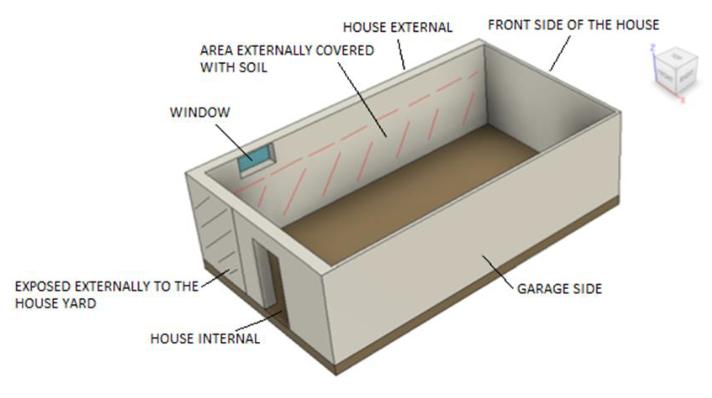
Figure 2.
Top view of the intake configurations.
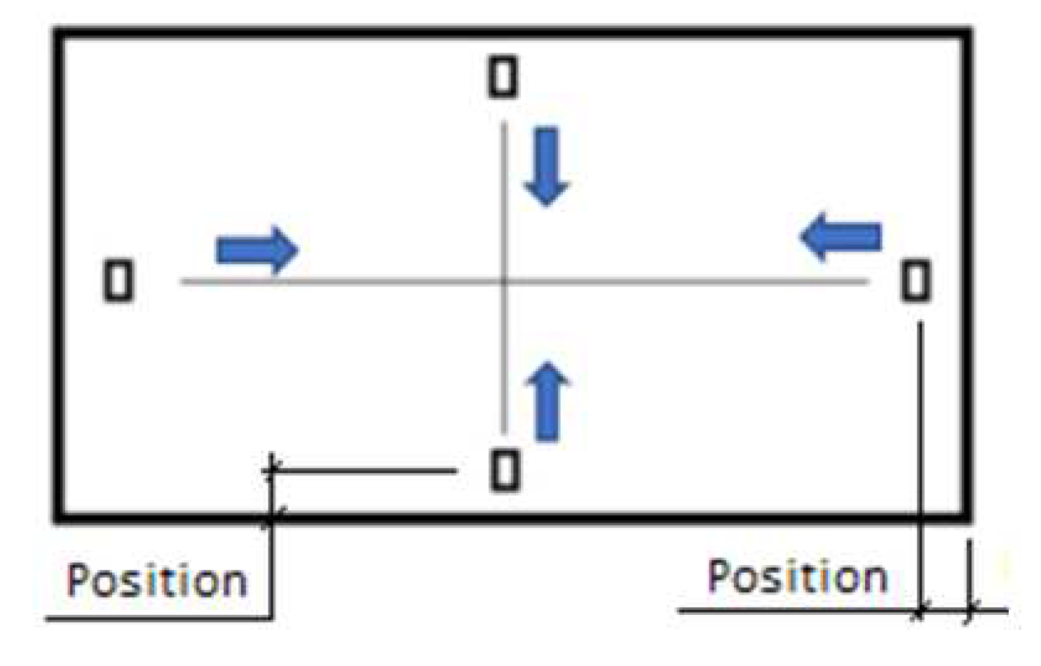
Figure 3.
Fitting of the experimental data to the model conforms to Equation (4).
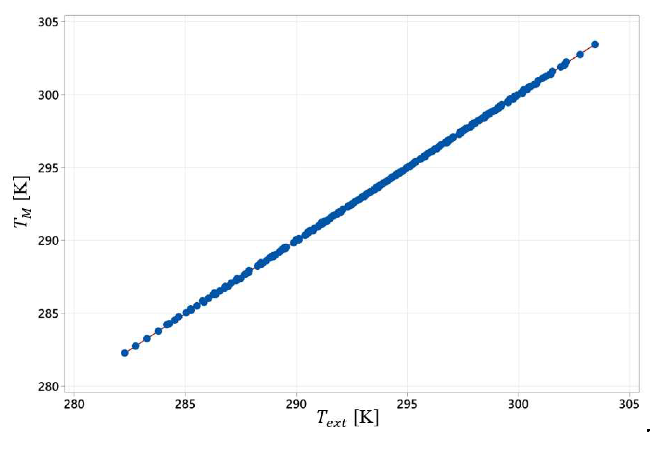
Figure 4.
Normality test for the Residue of the Model conforms to Equation (4).
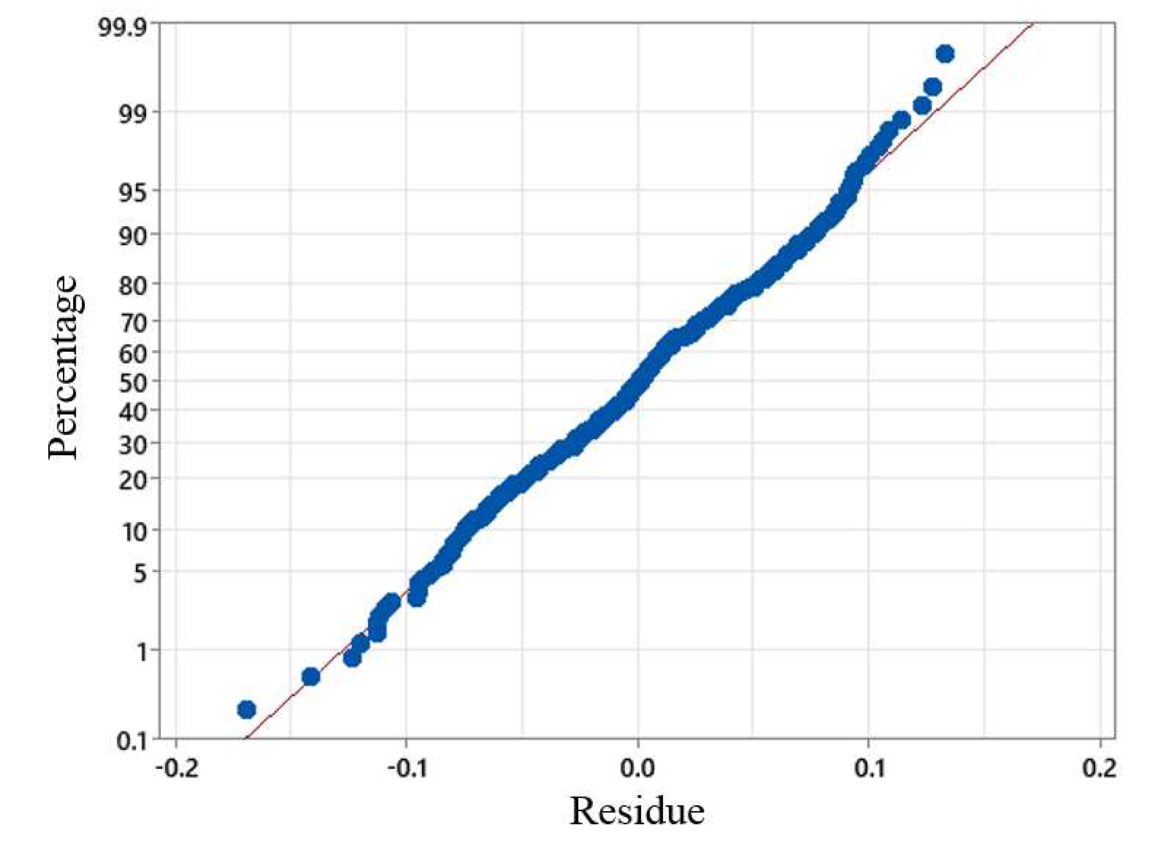
Figure 5.
Fitting the experimental points to the model conform to Equation (4), the generalization test.
Figure 5.
Fitting the experimental points to the model conform to Equation (4), the generalization test.
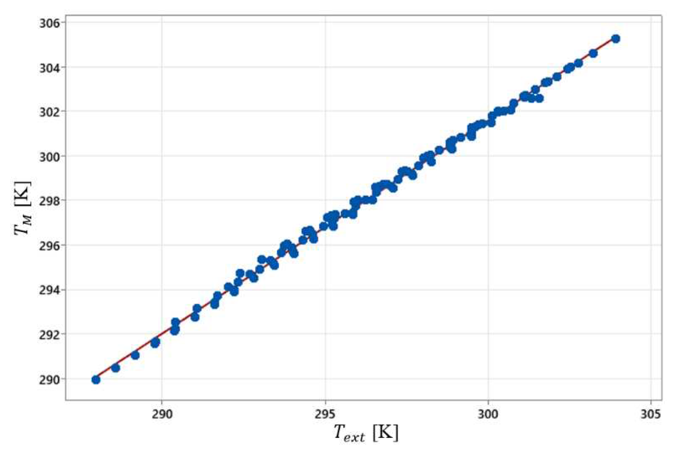
Figure 6.
Boundary graph for and as a function of experimental conditions, with m/s and .
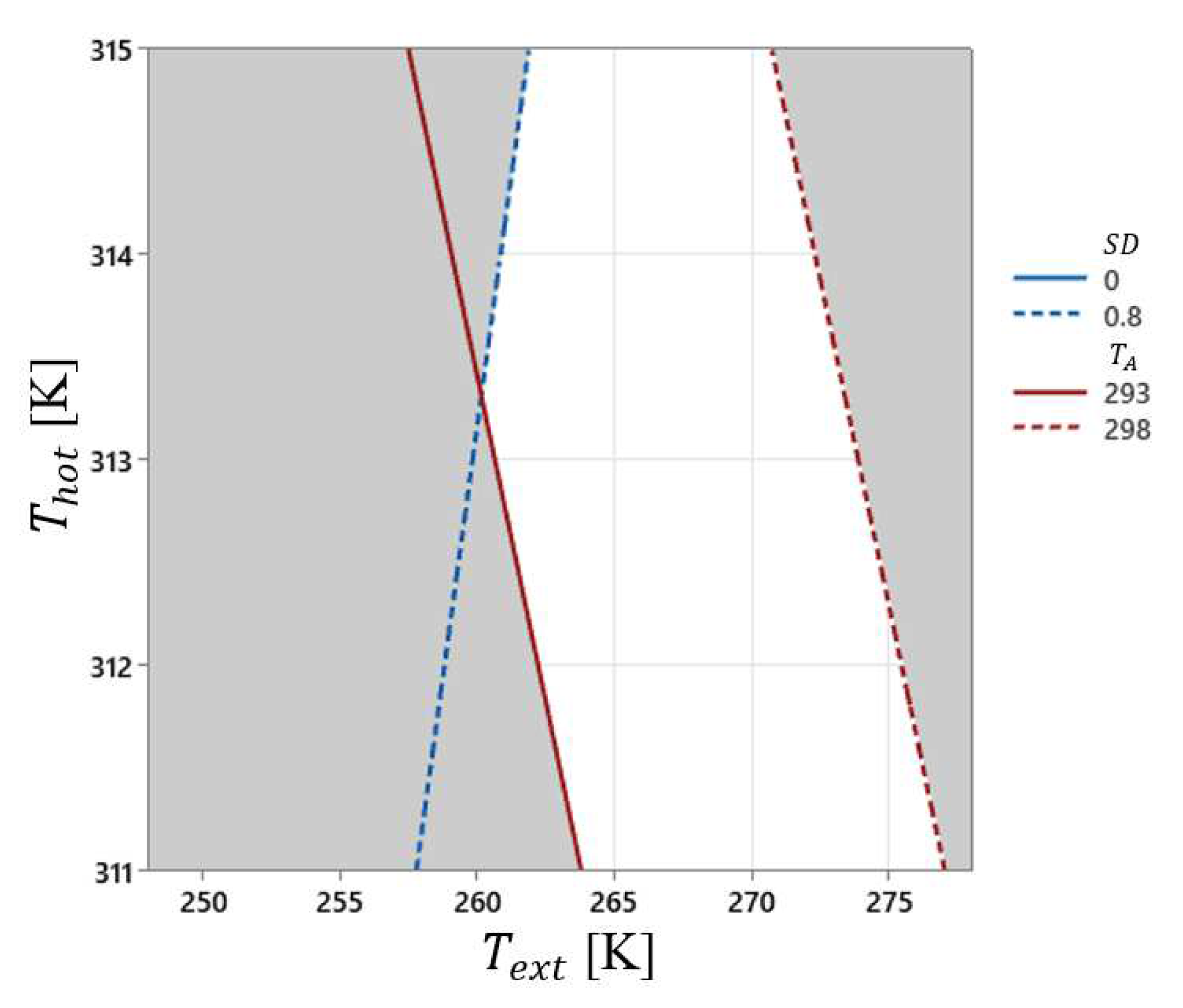
Figure 7.
Boundary graph for and as a function of experimental conditions, with m/s and .
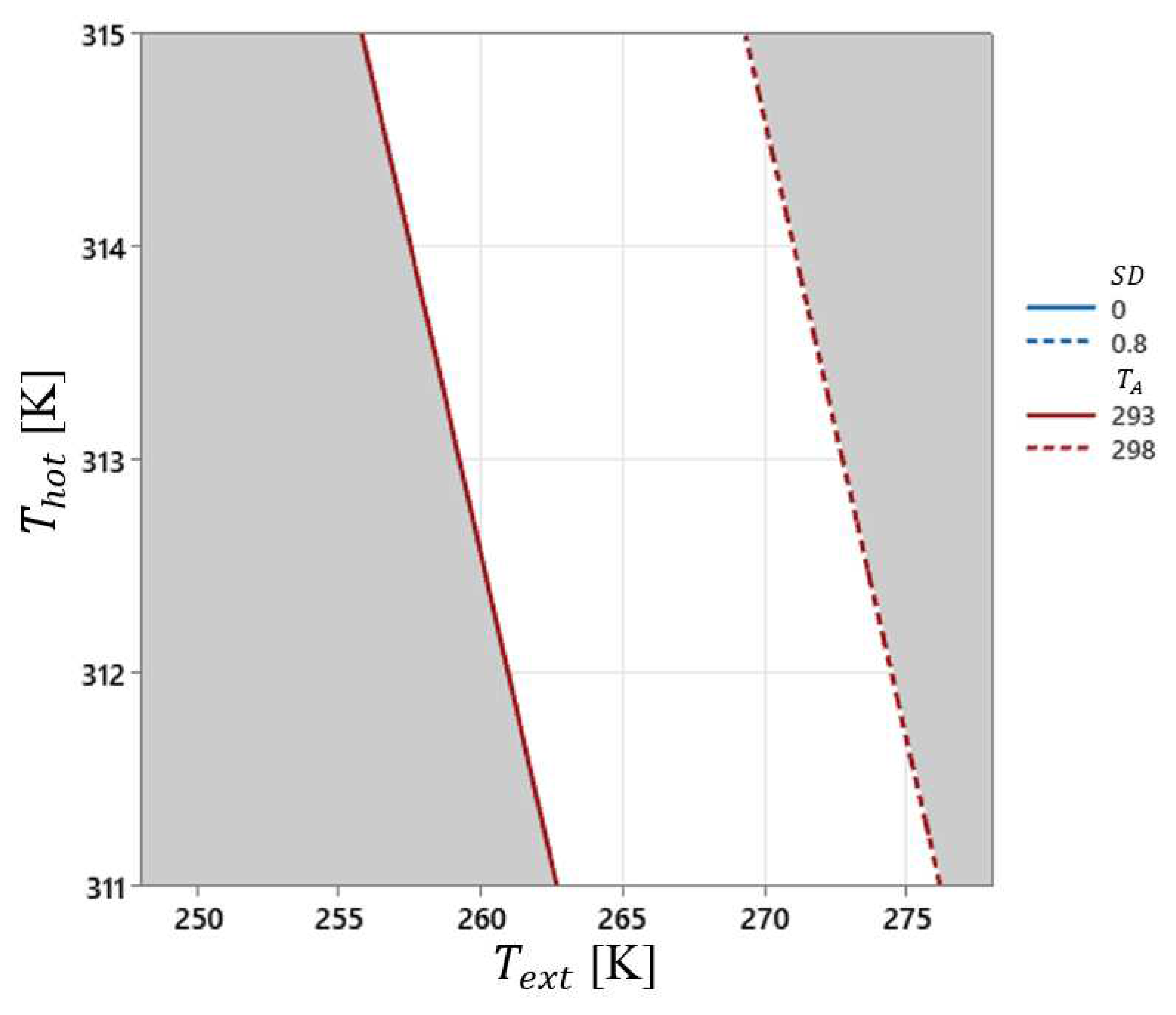
Figure 8.
Boundary graph for and as a function of experimental conditions, with m/s and .
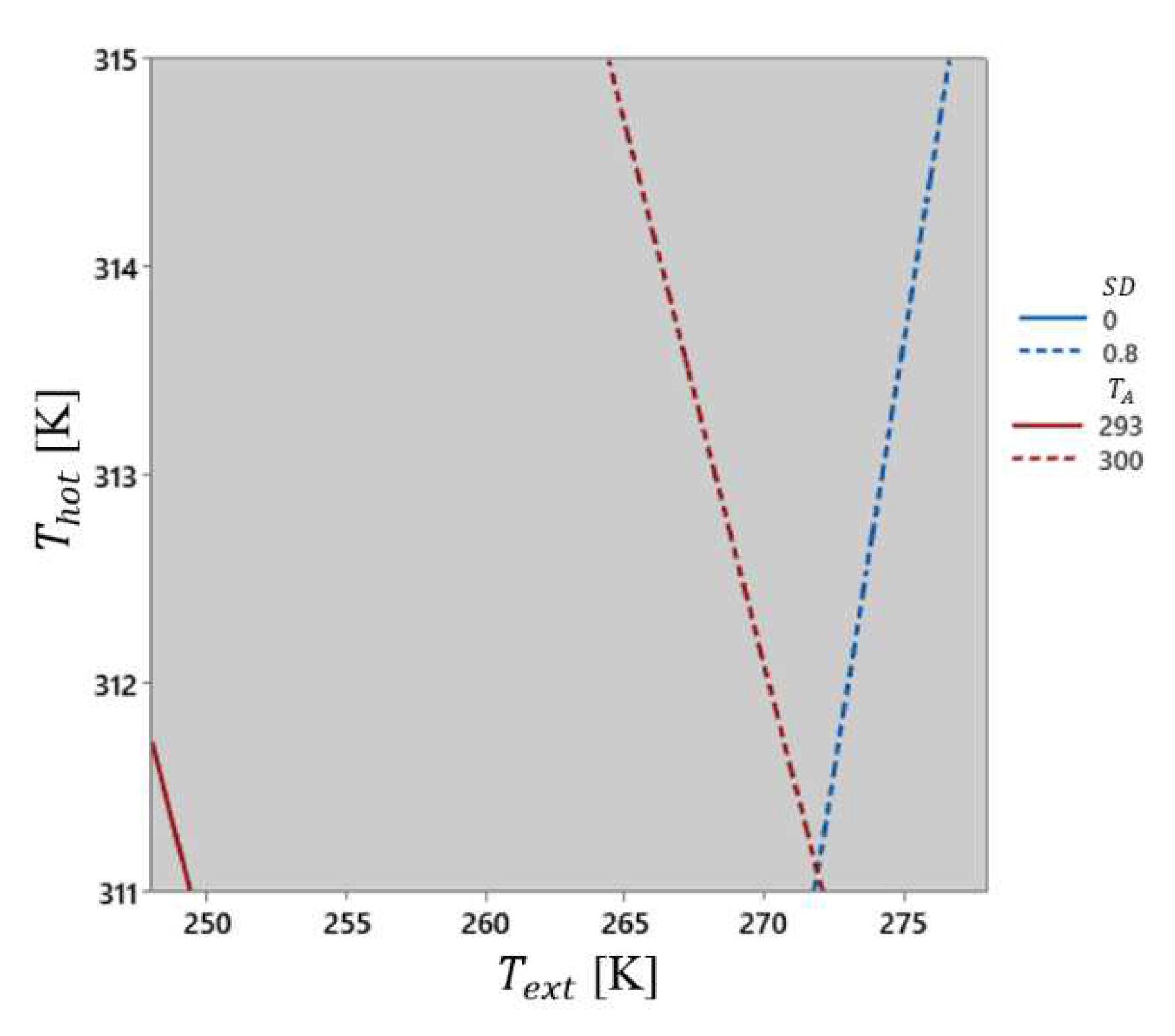
Figure 9.
Boundary graph for (293 – 298 K) and as a function of experimental conditions, with m/s and .
Figure 9.
Boundary graph for (293 – 298 K) and as a function of experimental conditions, with m/s and .
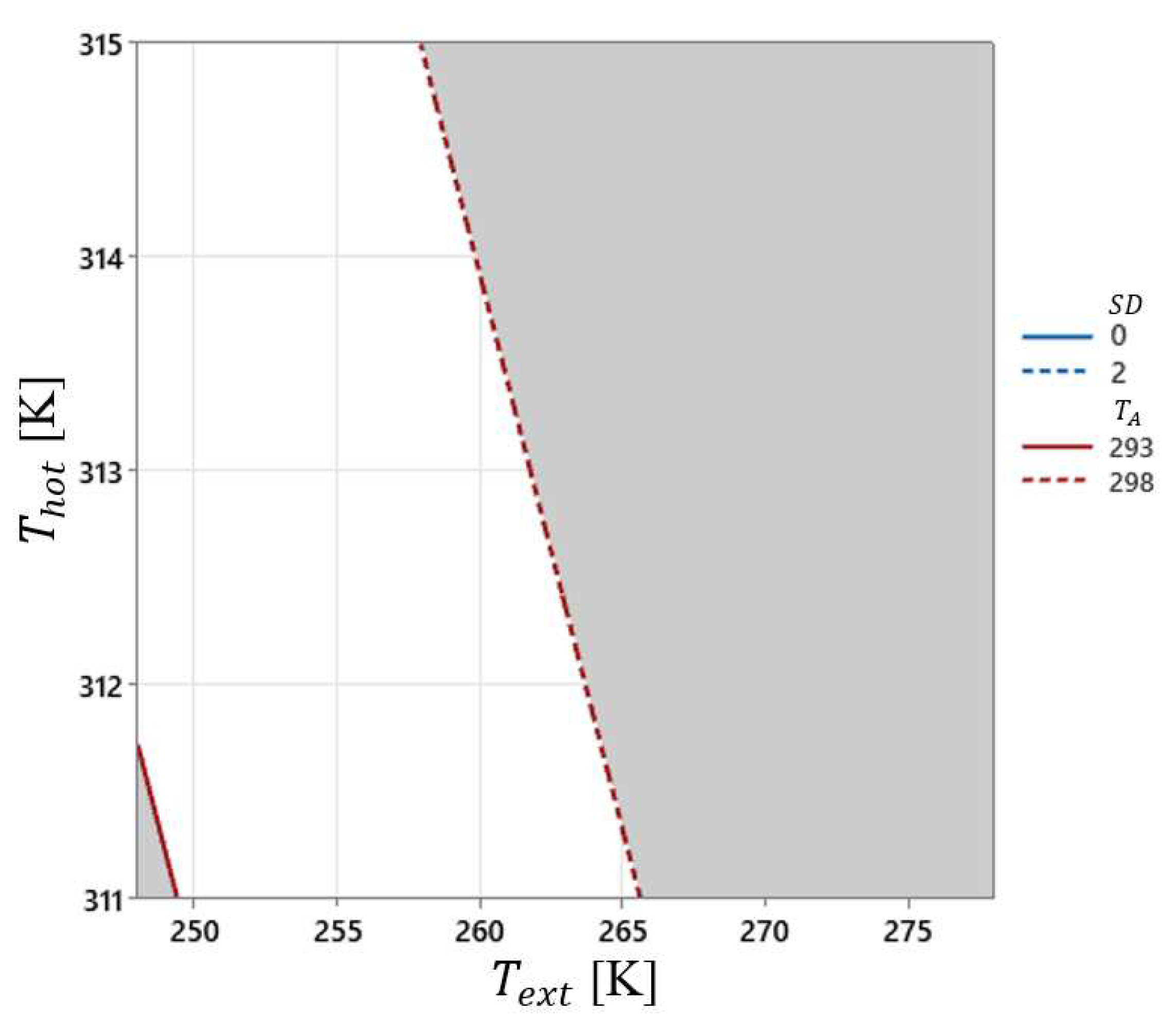
Figure 10.
Boundary graph for (293 – 300 K) and as a function of experimental conditions, with m/s and .
Figure 10.
Boundary graph for (293 – 300 K) and as a function of experimental conditions, with m/s and .
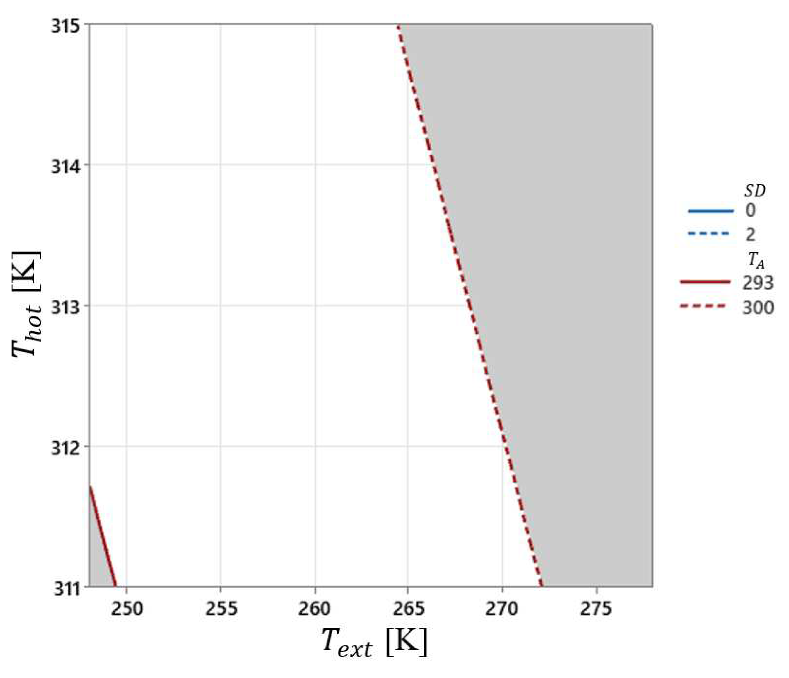

Table 1.
Statistics.
| Variable | N | Average | STDev | Minimum | Maximum |
|---|---|---|---|---|---|
| [K] | 308 | 263.00 | 10.02 | 248.00 | 278.00 |
| [K] | 308 | 313.00 | 1.43 | 311.00 | 315.00 |
| [m/s] | 308 | 2.5114 | 0.4064 | 2.0000 | 3.0000 |
| 308 | 4.886 | 4.064 | 0.000 | 10.000 |
STDev: standard deviation.
Table 2.
Analysis of the Variance Model conforms to Equation (4).
| Source | GL | SQ (Aj.) | QM (Aj.) | F-Value | p-Value |
|---|---|---|---|---|---|
| Regression | 10 | 6133.02 | 613.30 | 194614.79 | 0.000 |
| [K] | 1 | 4348.36 | 4348.36 | 1379834.22 | 0.000 |
| [K] | 1 | 221.84 | 221.84 | 70396.44 | 0.000 |
| [m/s] | 1 | 856.04 | 856.04 | 271641.78 | 0.000 |
| [%] | 1 | 563.83 | 563.83 | 178915.63 | 0.000 |
| [m2/s2] | 1 | 3.85 | 3.85 | 1221.97 | 0.000 |
| 1 | 4.50 | 4.50 | 1429.38 | 0.000 | |
| [K⋅m/s] | 1 | 33.93 | 33.93 | 10766.28 | 0.000 |
| [K] | 1 | 22.59 | 22.59 | 7167.28 | 0.000 |
| [K⋅m/s] | 1 | 0.71 | 0.71 | 226.50 | 0.000 |
| [m/s] | 1 | 1.40 | 1.40 | 442.96 | 0.000 |
| Error | 297 | 0.94 | 0.00 | ||
| Total | 307 | 6133.95 |
GL: degrees of freedom; SQ (Aj.): sum squared; QM (Aj.): medium sum squared; F-Value: F distribution value; p-Value: p value.
Table 3.
The summary of the quality of fitting of the Model conforms to Equation (4).
| S | R2 | R2(aj) | R2(pred) | 10-folds S | 10-folds R2 |
|---|---|---|---|---|---|
| 0.0561370 | 99.98% | 99.98% | 99.98% | 0.0578297 | 99.98% |
S: sum square; R2: R square; R2 (aj): R2 adjusted; 10-fold S: sum squared of the validation process 10 folds; 10-fold R2: R2 of the 10-fold validation process.
Table 4.
Analysis of the Model Variance conforms to Equation (4).
| Source | GL | SQ (Aj.) | QM (Aj.) | F-Value | p-Value |
|---|---|---|---|---|---|
| Regression | 13 | 16.8278 | 1.29444 | 6019.22 | 0.000 |
| [K] | 1 | 6.0999 | 6.09993 | 28364.92 | 0.000 |
| [K] | 1 | 0.1306 | 0.13065 | 607.51 | 0.000 |
| [m/s] | 1 | 0.1678 | 0.16777 | 780.13 | 0.000 |
| 1 | 3.1615 | 3.16154 | 14701.29 | 0.000 | |
| [m2/s2] | 1 | 0.0020 | 0.00197 | 9.14 | 0.003 |
| 1 | 0.0919 | 0.09190 | 427.34 | 0.000 | |
| [K⋅m/s] | 1 | 0.0229 | 0.02286 | 106.32 | 0.000 |
| [K] | 1 | 0.2329 | 0.23292 | 1083.09 | 0.000 |
| [K] | 1 | 0.0125 | 0.01250 | 58.14 | 0.000 |
| [m/s] | 1 | 0.2695 | 0.26946 | 1252.98 | 0.000 |
| [K⋅m/s] | 1 | 0.0106 | 0.01059 | 49.23 | 0.000 |
| [m2/s2] | 1 | 0.0023 | 0.00230 | 10.69 | 0.001 |
| [m/s] | 1 | 0.0134 | 0.01345 | 62.52 | 0.000 |
| Error | 294 | 0.0632 | 0.00022 | ||
| Total | 307 | 16.8910 |
GL: degrees of freedom; SQ (Aj.): sum squared; QM (Aj.): medium sum squared; F-Value: F distribution value; p-Value: p value.
Table 5.
The summary of the quality of fitting of the Model conforms to Equation (5).
| S | R2 | R2(aj) | R2(pred) | 10-folds S | 10-folds R2 |
|---|---|---|---|---|---|
| 0.0146647 | 99.63% | 99.61% | 99.59% | 0.0151341 | 99.58% |
S: sum square; R2: R square; R2(aj): R2 adjusted; 10-fold S: sum squared of the validation process 10 folds; 10-fold R2: R2 of the 10-fold validation process.
Disclaimer/Publisher’s Note: The statements, opinions and data contained in all publications are solely those of the individual author(s) and contributor(s) and not of MDPI and/or the editor(s). MDPI and/or the editor(s) disclaim responsibility for any injury to people or property resulting from any ideas, methods, instructions or products referred to in the content. |
© 2023 by the authors. Licensee MDPI, Basel, Switzerland. This article is an open access article distributed under the terms and conditions of the Creative Commons Attribution (CC BY) license (http://creativecommons.org/licenses/by/4.0/).
Copyright: This open access article is published under a Creative Commons CC BY 4.0 license, which permit the free download, distribution, and reuse, provided that the author and preprint are cited in any reuse.


