Effects on Soil Chemical Properties Two Years after Application of Compost in a Hedged Olive Grove

1. Introduction

Composting of organic waste of agricultural origin, and its application to the soil in arable lands is a good example of a measure of the Circular Economy, integrated in the European Green Deal. Indeed, composting of organic residues is a remarkable transforming process, capable of converting the problem of waste accumulation in a resourceful material with soil fertilizing and amending potential. Compost can increase the organic matter content of the soil, sequestering carbon, helping to mitigate climate change, improving various physical, chemical and biological properties of the soil, and when integrated in crop fertilization plans, can positively impact the economy and environment of farms by reducing the use of fertilizers and other agrochemicals [1–3].

Despite the great expansion of olive groves in Portugal in the last 20 years, and its large area of occupation in Spain (more than 0.352 M ha in Portugal and 2.5 M ha in Spain [4]), composting with olive generated products is not a widespread practice in both countries. Although there are some studies about the effects on soil of the use of olive mill wastewater and/or olive mill pomace [5–7] literature about composting of olive leaves, and studies about its effect on soils are much more scarce.

Besides the natural accumulation of olive leaves at soil surface, as a result of leaf fall and pruning, huge amounts of leaves are regularly produced by cleaning of olives before entering the olive mills. These leaves could be also spread at soil surface but, alternatively, can be used as bulking agent in composting mixture, to obtain a product with higher potential for soil amending and for soil C sequestration [7].

This study presents the results of a two-year field trial in a hedged olive grove, with the application of a compost of olive leaves and sheep manure, and it aims to assess: (i) short-term effects on soil, mainly on chemical properties, including on soil organic carbon and some soil organic matter components; (ii) the approach and methods used in detecting short-term effects in the soil, after spreading a compost in field conditions.

2. Materials and Methods

2.1. Site Characterization

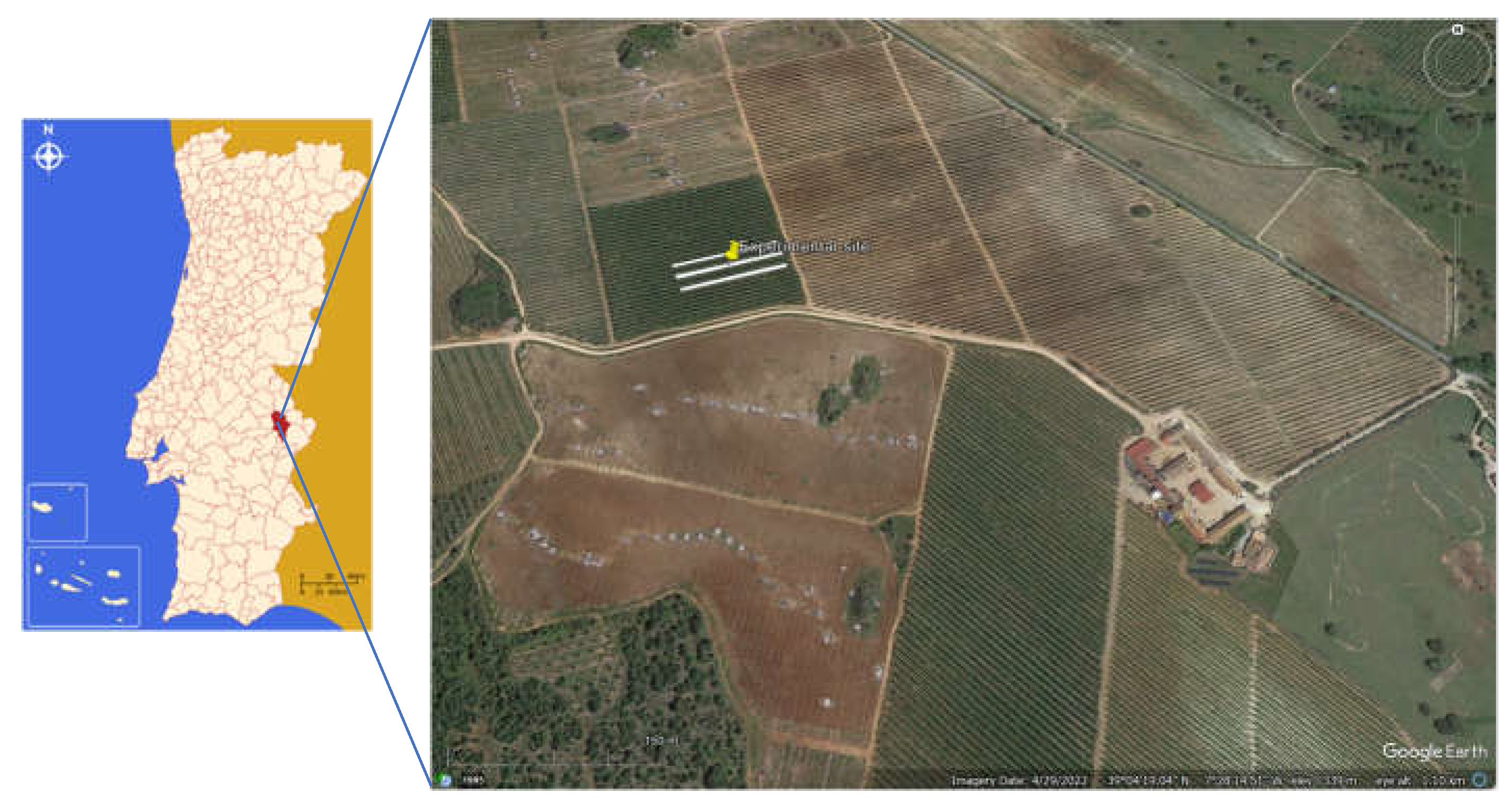
This experimental study was undertaken near Monforte, Portalegre district, Portugal (experimental field: 39° 4'9.23"N 7°27'59.33"W, Figure 1). The region has a Mediterranean climate, with mild short winters and hot dry summers (Csa climate by Köppen-Geiger). Climatological data (1981-2010) registered in the nearest meteorological station (Portalegre) shows an annually average air temperature of 15.2 °C, with monthly average temperatures varying from 8.6 °C in January to 24.1 °C in August. The annually average precipitation in the same period was 833 mm, varying from a minimum monthly average of 7 mm in July to a maximum of 128 mm in December [8].

Figure 1. Location of the experimental site.

Figure 1. Location of the experimental site.

For the region of the study, Table 1 shows air temperature (T) deviations from the climate normal temperature, and accumulated precipitation (R) ratios with normal precipitation, for the indicated quarters, during the time span of this study. Temperatures were quite above normal during almost the entire period. In 2020, the winter and autumn were quite wetter than normal, but 2021 and the beginning of 2022 were much dryer periods, which evolved to ‘severe’ drought declaration by February 2022 [9].

Table 1. Deviations between monthly air temperature (T) and accumulated precipitation (R) deviations from equivalent values in the period 1971-2000, for the quarters indicated in the region of Monforte (IPMA, 2023).

Years	Quarters (months initials)
	D // J-F		M-A-M		J-J-A		S-O-N
	T	R	T	R	T	R	T	R
2020	+2.0°C	0.88	+2°C	1.75	+1.25°C	0.13	+1.25°C	1.38
2021	-0.25°C	1.0	+2°C	0.63	+0.75°C	0.75	+0.0	0.88
2022	+1.5°C	0.30 *	-	-	-	-	-	-
*Meteorological drought declared: weak in Dec./2021, moderate in Jan/2022., and severe in Feb./2022.

Table 1. Deviations between monthly air temperature (T) and accumulated precipitation (R) deviations from equivalent values in the period 1971-2000, for the quarters indicated in the region of Monforte (IPMA, 2023).

Years	Quarters (months initials)
	D // J-F		M-A-M		J-J-A		S-O-N
	T	R	T	R	T	R	T	R
2020	+2.0°C	0.88	+2°C	1.75	+1.25°C	0.13	+1.25°C	1.38
2021	-0.25°C	1.0	+2°C	0.63	+0.75°C	0.75	+0.0	0.88
2022	+1.5°C	0.30 *	-	-	-	-	-	-
*Meteorological drought declared: weak in Dec./2021, moderate in Jan/2022., and severe in Feb./2022.

The experimental trial set up for this study is located in a gentle slope (2-5% slope gradient) approximately SW-NE oriented (Figure 1). Dominant soils are Skeletic Regosol and Vertic Luvisol, both with intermediate textures (loam to clay loam) in the superficial horizons and with occasional occurrence of carbonates, especially in deeper layers, but that can appear near soil surface as result of previous deep soil tillage [10]. The field trial was installed in 2020 in a hedged olive grove (Olea europaea L., cv. ‘Cobrançosa’), six years old, which has been managed to achieve high production standards. Soil management adopted include drip irrigation, regular soil fertilization, no tillage (since 2014), weed control by mechanical means in the interrow, and by herbicide in the row.

2.2. Experimental Layout and Soil Sampling

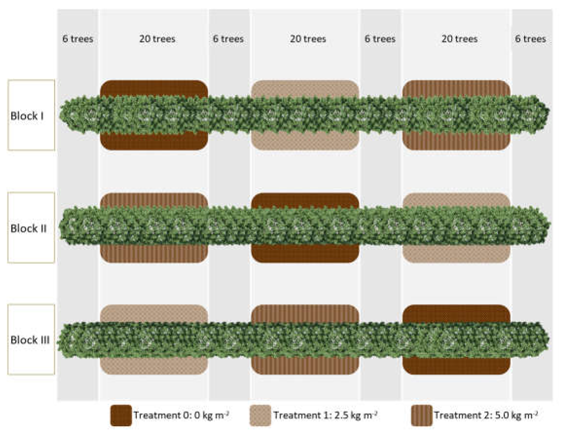
The experimental layout is a randomized complete block with three blocks (replicates) each one with three treatments (one replicate per block), giving a total of 9 plots (Figure 2). Each block (I, II, and III) consisted in one line of trees, divided in three consecutive plots. Each plot is formed by 20 olive trees separated from the following plot by six border trees. Two tree rows border consecutive blocks (not represented in Figure 2). This olive grove has a tree spacing of 6.5 m x 1.5 m (6.5 m between tree rows and 1.5 m between trees in the same row) and plots have approximately 60 m² (30 m x 2 m, ~1 m each side the row – see Section 2.3). The three plots in each block were randomly allocated to one of the three nominal dosages of compost (treatments): T0 or control (0 kg m^-2), T1 (2.5 kg m^-2), and T2 (5.0 kg m^-2) – Figure 3.

Figure 2. Experimental setup and compost dosages: T0 or control (0 kg m^-2), T1 (2.5 kg m^-2), and T2 (5.0 kg m^-2). There are two tree lines between each block and 6.5 m spacing between each tree line.

Figure 2. Experimental setup and compost dosages: T0 or control (0 kg m^-2), T1 (2.5 kg m^-2), and T2 (5.0 kg m^-2). There are two tree lines between each block and 6.5 m spacing between each tree line.

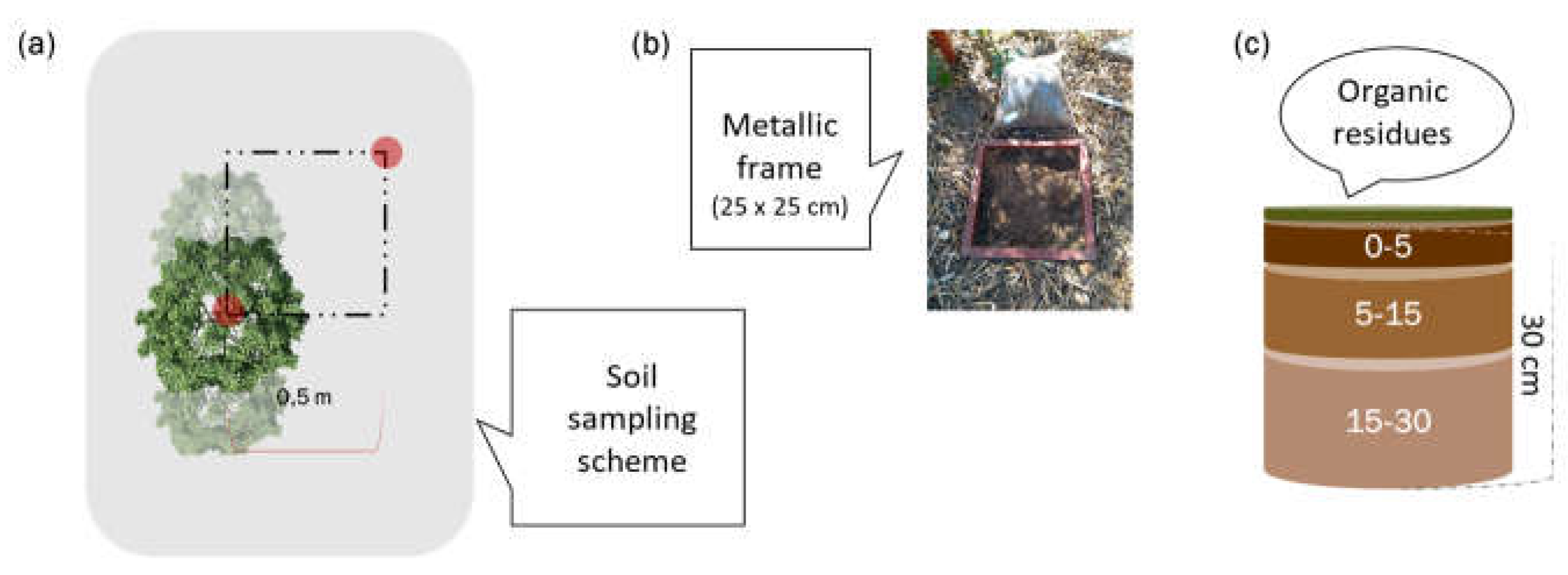
Soil sampling in each plot was carried out by randomization of the trees, both for disturbed and undisturbed soil samples. Tree position was assumed as being at the vertex of a 0.5 m square and soil samples were collected at the opposite vertex (Figure 4a). Organic residues and undisturbed soil samples were collected from an area delimited with a 25 x 25 cm² metallic frame (four samples per plot, total N = 36, Figure 4b). Considering that the compost was applied as a mulch at soil surface, in order to maximize the detection of short-term soil changes, three soil layers of increasing thickness were sampled (0-5 cm, 5-15 cm, and 15-30 cm, Figure 4c). One composite soil sample per plot and layer was collected, from a minimum of 12 sampling points extracted with a hand probe equally distributed on both sides of the tree row.

Figure 3. Disturbed and undisturbed soil sampling schemes in each tree line.

Figure 3. Disturbed and undisturbed soil sampling schemes in each tree line.

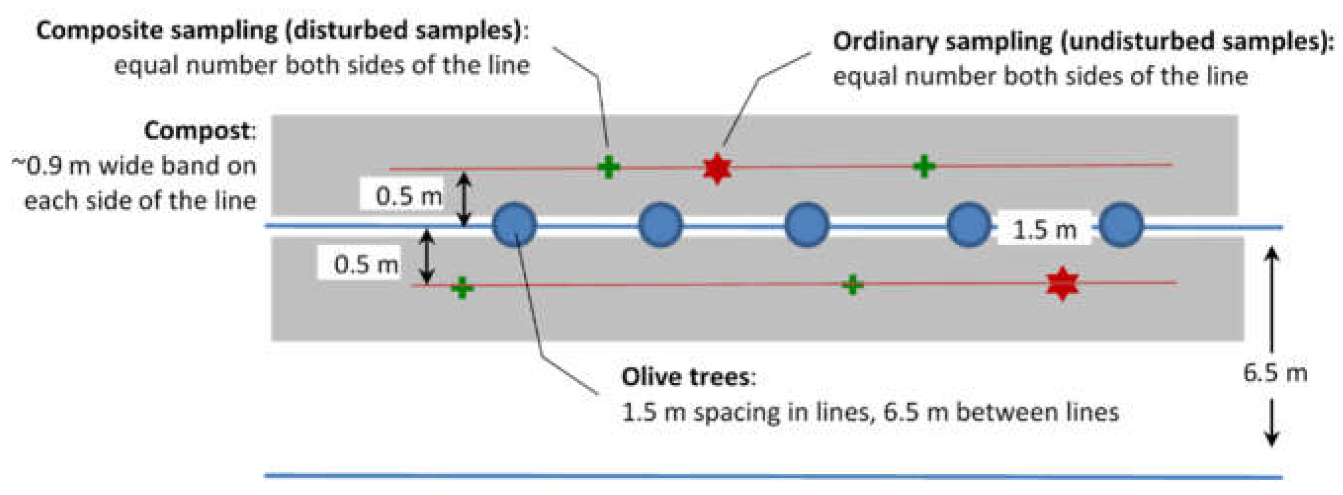
Figure 4. Soil sampling position in relation to the nearest tree (a); metallic frame used for organic residues collection (b); and depths of soil layers adopted (c).

Figure 4. Soil sampling position in relation to the nearest tree (a); metallic frame used for organic residues collection (b); and depths of soil layers adopted (c).

The compost addition was carried out at the end of February 2020, and soil samplings were done (i) before that, at the beginning of 2020, and approximately (ii) one year (2021.03), and (iii) two years (2022.01) after the soil amendment.

2.3. Compost

The compost was produced on the farm in a four-month duration process (June to September 2019), using leaves and twigs resulting from the olives cleaning, before entering the mill, and sheep manure (Figure 4a) in a 2:1 proportion of these two components, respectively. After maturation, analysis of the compost revealed the following main characteristics and composition [11]: 424 g kg^-1 of moisture, pH 8.4, 124 g kg^-1 organic C, C/N ratio of 11.8, 5.1 g kg^-1 P₂O₅, 6.1 g kg^-1 K₂O, 155 mg kg^-1 Cu, and 219 mg kg^-1 Zn.

The compost was applied in February 2020 with a manure spreader (Herculano H2RSP) adapted and previously tested for its distribution at soil surface in a strip of ~0.9 m width, each side of the trees row (Figure 4b).

Figure 4. Compost preparation (a) and field view after the application of the compost (b).

Figure 4. Compost preparation (a) and field view after the application of the compost (b).

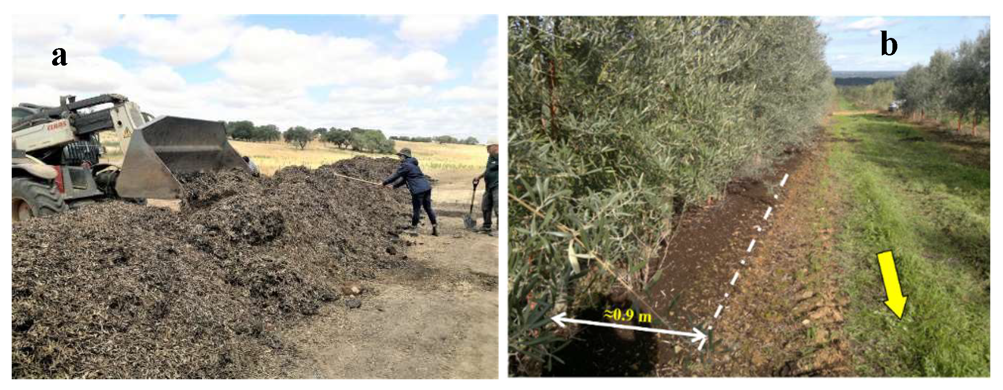
To report the applied compost dosages to larger area units, i.e. ha^-1, we should consider the effective area where it has been applied. Therefore, assuming that the compost is applied in strips of 1.8 m, extending approximately 0.9 m each side of the trees row (Figure 4b), with a 6.5 m spacing, it means the area covered by the compost represents ~0.28 ha ha^-1. Consequently, the dosage T1 (2.5 kg m^-2) corresponds to 7 Mg ha^-1, and T2 (5.0 kg m^-2) to 14 Mg ha^-1. The same conversion must be applied to quantitative soil effects due to the compost, if they are to be reported at crop field scale.

2.4. Laboratory Methods and Calculations

Organic residues at soil surface (amendment, when applied, and natural occurring residues) were air dried, sieved with a 1 mm mesh sieve, oven dried at 65°C, weighted and expressed as dry mass of organic residues >1 mm (kg m^-2).

Bulk density of the 0-5 cm soil layer was monitored by the cylinder method [12] in 2020, 2021 and 2022. An undisturbed soil core was collected in a 100 cm3 metal cylinder and bulk density was determined dividing the oven dried (105°C) mass of the soil sample by the volume of the cylinder. Bulk density of the 5-15 and 15-30 cm soil layers were determined only before the compost addition to allow soil C-stock determinations. With the compost applied at soil surface, it was assumed the bulk density of the lower layers would be kept constant during the two years period of the study.

Composite soil samples were air dried and sieved to separate the rock fragments (> 2 mm) from the soil fine fraction (< 2 mm). Rock fragments were washed, oven dried at 105°C, weighted, and expressed per total soil sample weight (g kg^-1). Soil texture of the fine fraction was determined using sieving and the pipette method. Rock fragments and soil texture were determined once, for soil characterization of the experimental plots.

Soil organic carbon (SOC) and total nitrogen (only sample collected in 2021) were determined by dry combustion and elemental analysis. Whenever detected, samples were previously submitted to carbonates removal following Leco’s recommended procedure.

The soil C stock is expressed as C mass for each layer and for the 0-30 cm layer, per area (kg m^-2). The C stock calculation took in consideration rock fragments to correct both, soil bulk density and volume of the soil fine fraction, following [13]. The bulk density of the fine fraction, BD_ff (g cm^-3) is given by:

$${BD}_{ff}=\frac{M_S-M_{RF}}{V_T-M_{RF}/2.65}$$

(1)

where M_S is the dry mass of the soil sample (g), M_RF is the mass of the rock fragments in the soil sample (g), V_T is the soil sample volume (cm³) and 2.65 is the rock fragments density (g cm^-3). Then, the C_stock (kg m^-2) can be obtained by:

$$C_{stock}=SOC\ast {BD}_{ff}\ast z\ast \left(1-{RF}_m\frac{{BD}_S}{2.65}\right)\ast 10$$

(2)

where SOC is the soil organic carbon (g g^-1), BD_ff is given by Equation (1), z is the thickness of the soil layer (cm), RF_m is the rock fragments as mass of particles > 2 mm per mass of total soil (g g^-1), BD_S is the soil bulk density (g cm^-3), and 10 converts the result to kg m^-2.

Quantification of the C-stock in the layer 0-5 cm used RF_m data (Table 2) and BD_S (Table 4) with differentiated values for each plot. This way we also admitted the incorporation of possible effects of the compost on the BD_S and BD_ff, which justified a more detailed monitoring of these variables in this layer, along with the SOC determination. To calculate the C-stock for layers 5-15 cm and 15-30 cm, variables RF, BD_S, and BD_ff were averaged for the entire experimental field, assuming that they would not be significantly affected by the compost addition during the time span of the study. Therefore, the C-stock variations between treatments, in the second- and third-layers, depend only on the SOC values. The following average values were adopted, respectively for layers 5-15 cm and 15-30 cm (Table 2 and 4): 108 and 91 g kg^-1 for RF, 1.32 and 1.34 g cm^-3 for BD_S, and 1.24 and 1.28 g cm^-3 for BD_ff.

Carbon of the particulate organic matter (POM-C) is the carbon content of the soil organic matter retained in a 0.53 mm mesh sieve [14,15]. Like for SOC, PAM-C was determined by dry combustion and elemental analysis, after carbonate removal whenever justified.

Permanganate oxidizable carbon (POX-C) was determined accordingly with the procedure of [16,17] and is expressed in mg kg^-1.

Both soil pH_H2O and soil pH_KCl were measured by potentiometry, the first one in a suspension of soil and distilled water (ratio 1:2.5) and the second one in a suspension of soil and 1N KCl solution (ratio 1:2.5).

Extractable phosphorus and potassium were determined by the Egnér-Riehm method (ammonium lactate) [18]. Extractable micronutrients cations (Fe, Mn, Zn, Cu) were determined by the Lakanen method [19] (ammonium acetate, acetic acid and EDTA). All nutrients are expressed in mg kg^-1 soil (fraction < 2 mm)

2.5. Statistical Analysis

For each sampling date and each studied soil variable, the homoscedasticity of the variances was confirmed by the Fligner test, the analysis of variance was carried out and, whenever the hypothesis of equality of means had P<0.05, the means were compared by the multiple test of Tukey. The R software [20] was used for all statistical analyses.

3. Results

3.1. Soil Texture of the Experimental Field

Table 2 presents soil texture data of the plots randomly allocated to each treatment (T0, T1 and T2). Although there is some variability of the soil texture among the treatments, neither the coarse fraction (rock fragments > 2 mm) nor the particle classes of the soil fine fraction (< 2mm) revealed statistically significant differences in each layer. Soil texture differences are small enough to have just two texture classes represented. Soils with T2 treatment are the most homogeneous with all three layers being clay loam, and plots having T0 and T1 treatments are both slightly coarser, with just one clay loam layer, but located in opposite depths: in T0 is the superficial layer (0-5 cm) and in T1 is the deeper layer (15-30 cm). Maximum range of the particle classes among all plots and soil layers occurred in the 0-5 cm layer: 104 g kg^-1 for sand, 44 g kg^-1 for silt, and 107 g kg^-1 for clay.

Table 2. Soil texture of the plots with treatments T0 (0 kg m^-2), T1 (2.5 kg m^-2), and T2 (5.0 kg m^-2): coarse fraction (> 2 mm) content (g kg^-1) and texture classes of the fine fraction (< 2 mm).

	Rock fragments (> 2 mm)							Texture classes**
Layer	T0		T1		T2			T0	T1	T2
(cm)	m	s	m	s	m	s
00-05	118.2	31.7	116.2	31.1	120.0	41.3		Clay loam	Loam	Clay loam
05-15	125.7	36.9	88.0	44.6	109.7	16.6		Loam	Loam	Clay loam
15-30	104.7	28.0	81.0	20.8	88.3	26.9		Loam	Clay loam	Clay loam

* mean (m) and standard deviation (s) of three plots per treatment (12 samples/treatment (4 samples/plot) in layer 0-5 cm, and one composite sample per plot in layers 5-15 and 15-30 cm); ** No statistically significant differences between treatments for each size particle class (coarse sand, fine sand, silt and clay).

Table 2. Soil texture of the plots with treatments T0 (0 kg m^-2), T1 (2.5 kg m^-2), and T2 (5.0 kg m^-2): coarse fraction (> 2 mm) content (g kg^-1) and texture classes of the fine fraction (< 2 mm).

	Rock fragments (> 2 mm)							Texture classes**
Layer	T0		T1		T2			T0	T1	T2
(cm)	m	s	m	s	m	s
00-05	118.2	31.7	116.2	31.1	120.0	41.3		Clay loam	Loam	Clay loam
05-15	125.7	36.9	88.0	44.6	109.7	16.6		Loam	Loam	Clay loam
15-30	104.7	28.0	81.0	20.8	88.3	26.9		Loam	Clay loam	Clay loam

* mean (m) and standard deviation (s) of three plots per treatment (12 samples/treatment (4 samples/plot) in layer 0-5 cm, and one composite sample per plot in layers 5-15 and 15-30 cm); ** No statistically significant differences between treatments for each size particle class (coarse sand, fine sand, silt and clay).

3.2. Organic Residues at Soil Surface

The mass of the organic residues bigger than 1 mm are presented in Table 3, including one additional sampling date: 07.2020, five months after the amendment application.

As it could be expected, there were no significant differences between the plots allocated to the treatments before the addition of the compost (02.2020). On the contrary, five months later (07.2020) the differences are quite expressive, especially between T2 and T0 and between T2 and T1 – the difference between T1 and T0, though evident, is not statistically significant.

There was a large reduction in the mass of organic residues from 2020 to 2021 in T1 and T2, though maintaining the same statistically significant differences as in the previous sampling moment (07.2020). From 2021 to 2022, there is only a reduction in the highest dose (T2) and no significant differences were found between treatments.

Table 3. Dry mass (65°C) of organic residues (> 1 mm) at soil surface (kg m^-2) for treatments T0 (0 kg m^-2), T1 (2.5 kg m^-2), and T2 (5.0 kg m^-2).

Sampling	T0		T1		T2
date	m*	s*	m	s	m	s
02.2020	0.77	0.29	0.54	0.23	0.69	0.35
07.2020	1.26a	0.78	3.08a	1.10	6.57b	3.72
03.2021	0.97a	0.43	1.28a	0.32	3.12b	1.25
01.2022	1.25	0.33	1.50	0.93	1.84	0.97

* mean (m) and standard deviation (s) of 12 samples/treatment (n = 4/plot); a, b… values with the same letter within a line have a P≤0.05 of being equal means.

Table 3. Dry mass (65°C) of organic residues (> 1 mm) at soil surface (kg m^-2) for treatments T0 (0 kg m^-2), T1 (2.5 kg m^-2), and T2 (5.0 kg m^-2).

Sampling	T0		T1		T2
date	m*	s*	m	s	m	s
02.2020	0.77	0.29	0.54	0.23	0.69	0.35
07.2020	1.26a	0.78	3.08a	1.10	6.57b	3.72
03.2021	0.97a	0.43	1.28a	0.32	3.12b	1.25
01.2022	1.25	0.33	1.50	0.93	1.84	0.97

* mean (m) and standard deviation (s) of 12 samples/treatment (n = 4/plot); a, b… values with the same letter within a line have a P≤0.05 of being equal means.

Based on the data for the control (T0), there was an increase of 0.49 kg m^-2 of organic residues in this five-month period. This increase of the litter layer can be mainly attributed to an occurrence of ‘olive peacock spot’ disease (Spilocaea oleaginea) which caused above normal leaf fall during the spring of 2020 (local staff oral communic.). Assuming that this leaf fall was approximately uniform in all field trial, making the difference of the mean values of T1 and T2 to the control (T0), it gives estimates of 1.82 and 5.31 kg m^-2 of compost (dry mass) for T1 and T2, respectively. Converting the compost dry mass to fresh mass (average moisture ~225 g kg^-1), we get ~2.25 and ~6.50 kg m^-2, respectively for T1 and T2. While the value for T1 is about 11% below the aimed nominal value (2.50 kg m^-2), for T2 the compost applied is about 30% above the nominal value (5.00 kg m^-2). We have also to consider two effects that contribute to underestimate the mass of the compost by this method: only the residues > 1 mm were quantified, and the time spanning of 5 months during a warmer and more humid spring than normal (Table 1) which should have already reduced its mass. Therefore, it is admissible that while for T1 the dosage should have been very close to the nominal value, for T2 it should have been above the intended nominal value. In fact, there were some difficulties with the mechanical spreading of the compost, especially for the higher dosage (T2), due to aggregation and formation of big blocks. This could have led to a more heterogeneous distribution at soil surface, which could explain the highest standard deviation observed in 07.2020, for dosage T2 (Table 3).

3.3. Bulk density

The soil bulk density (BD_S) did not register significant differences in the plots where the three compost dosages (T0, T1 and T2) were applied, both before, and one year after the compost addition (Table 4). Only after two years (2022) a significant lower soil density was detected in the plots where the T2 dosage was applied, compared to the T0 and T1 dosages. However, discounting the coarse fraction (> 2 mm), the systematic reductions of the fine fraction bulk density (< 2 mm, BD_ff), observed for T1 and T2, both in 2021 and 2022, were not statistically significant.

Table 4. Soil bulk density (BD_S) and bulk density of the fine fraction (< 2 mm, BD_ff) of the layer 0-5 cm, for treatments T0 (0 kg m^-2), T1 (2.5 kg m^-2), and T2 (5.0 kg m^-2).

Sampling	BDS (g cm-3)							BDff (g cm-3)
year	T0		T1		T2			T0		T1		T2
	m*	s*	m	s	m	s		m	s	m	s	m	s
2020	1.291	0.142	1.338	0.117	1.317	0.123		1.216	0.020	1.258	0.076	1.241	0.011
2021	1.304	0.080	1.307	0.097	1.306	0.077		1.257	0.095	1.249	0.081	1.233	0.074
2022	1.383a	0.089	1.314a	0.089	1.290b	0.096		1.313	0.098	1.248	0.099	1.223	0.124

* mean (m) and standard deviation (s) of 12 samples per treatment (4 samples/plot); a, b… values with the same letter within a line have a P≤0.05 of being equal means.

Table 4. Soil bulk density (BD_S) and bulk density of the fine fraction (< 2 mm, BD_ff) of the layer 0-5 cm, for treatments T0 (0 kg m^-2), T1 (2.5 kg m^-2), and T2 (5.0 kg m^-2).

Sampling	BDS (g cm-3)							BDff (g cm-3)
year	T0		T1		T2			T0		T1		T2
	m*	s*	m	s	m	s		m	s	m	s	m	s
2020	1.291	0.142	1.338	0.117	1.317	0.123		1.216	0.020	1.258	0.076	1.241	0.011
2021	1.304	0.080	1.307	0.097	1.306	0.077		1.257	0.095	1.249	0.081	1.233	0.074
2022	1.383a	0.089	1.314a	0.089	1.290b	0.096		1.313	0.098	1.248	0.099	1.223	0.124

* mean (m) and standard deviation (s) of 12 samples per treatment (4 samples/plot); a, b… values with the same letter within a line have a P≤0.05 of being equal means.

The organic matter as a lowering effect in the soil bulk density that is well known. It is the result of the lower density of the organic matter itself, but also a consequence of the higher stability of the aggregates and of its complementary pore network, namely that created by the biological activity usual enhanced by higher levels of organic matter. However, these effects take time, and even more with the applied organic material concentrated at soil surface as a mulch. Therefore, it seems two years may be an insufficient lapse of time to generate unequivocally bulk density changes, in the soils and environmental conditions of this study.

3.4. Soil Organic Carbon and C-Stock

As shown in Table 5, before the application of the compost (2020) the SOC mean for the plots assigned to treatments T0, T1 and T2 were not statistically different (P<0.05), for all layers. However, the SOC mean of the layer 0-5 cm, in the plots allocated to T2 was lower than the SOC observed in plots allocated to T0, having a P<0.10 of both means being equal, by chance.

One year after the compost spreading (2021), there were no significant differences in the SOC mean between all treatments, and for all the three layers. At least in part, this might be due to the high variability of the data, especially in the T2 treatment. After two years some significant differences emerge, mainly between T2 and T0 in the layer 5-15 cm depth. But also, in the first layer, the probability of T2 and T0 having an equal SOC mean is very low (P<0.10).

The 15-30 cm layer seems to show just random SOC fluctuations in all treatments.

Table 5. Soil organic carbon (SOC) and C-stock in each soil layer for treatments T0 (0 kg m^-2), T1 (2.5 kg m^-2), and T2 (5.0 kg m^-2).

Layer	SOC (g kg-1)							C-stock (kg m-2)
(cm)	T0		T1		T2			T0		T1		T2
	m*	s*	m	s	m	s		m	s	m	s	m	s
	2020
00-05	17.0a’	1.1	16.3a	1.0	14.5a’	0.8		0.977	0.080	0.970	0.136	0.851	0.059
05-15	12.1	1.6	12.3	0.2	12.9	0.7		1.423	0.191	1.439	0.025	1.517	0.078
15-30	8.8	1.7	8.7	0.2	9.4	1.0		1.618	0.305	1.600	0.028	1.722	0.191
	2021
00-05	15.5	0.7	16.7	0.8	17.3	2.1		0.913	0.020	0.985	0.054	0.999	0.149
05-15	11.4	1.2	12.4	0.7	13.2	0.6		1.342	0.142	1.455	0.082	1.545	0.065
15-30	8.7	1.1	8.8	0.3	9.1	0.1		1.594	0.198	1.618	0.046	1.667	0.019
	2022
00-05	15.7a’	0.7	17.1a	1.0	18.2a’	1.6		0.960	0.048	1.003	0.064	1.054	0.167
05-15	11.6a	1.3	12.5ab	0.4	13.7b	0.5		1.361a	0.153	1.467a	0.047	1.611b	0.059
15-30	9.0	1.1	8.8	0.7	8.8	0.3		1.649	0.208	1.612	0.120	1.655	0.059

* mean (m) and standard deviation (s) of three plots per treatment (one composite sample per plot). a, b… values with the same letter within a line have a P≤0.05 of being equal means, and with the same letter with an apostrophe (a’, b’…) have a P<0.10 of being equal means.

Table 5. Soil organic carbon (SOC) and C-stock in each soil layer for treatments T0 (0 kg m^-2), T1 (2.5 kg m^-2), and T2 (5.0 kg m^-2).

Layer	SOC (g kg-1)							C-stock (kg m-2)
(cm)	T0		T1		T2			T0		T1		T2
	m*	s*	m	s	m	s		m	s	m	s	m	s
	2020
00-05	17.0a’	1.1	16.3a	1.0	14.5a’	0.8		0.977	0.080	0.970	0.136	0.851	0.059
05-15	12.1	1.6	12.3	0.2	12.9	0.7		1.423	0.191	1.439	0.025	1.517	0.078
15-30	8.8	1.7	8.7	0.2	9.4	1.0		1.618	0.305	1.600	0.028	1.722	0.191
	2021
00-05	15.5	0.7	16.7	0.8	17.3	2.1		0.913	0.020	0.985	0.054	0.999	0.149
05-15	11.4	1.2	12.4	0.7	13.2	0.6		1.342	0.142	1.455	0.082	1.545	0.065
15-30	8.7	1.1	8.8	0.3	9.1	0.1		1.594	0.198	1.618	0.046	1.667	0.019
	2022
00-05	15.7a’	0.7	17.1a	1.0	18.2a’	1.6		0.960	0.048	1.003	0.064	1.054	0.167
05-15	11.6a	1.3	12.5ab	0.4	13.7b	0.5		1.361a	0.153	1.467a	0.047	1.611b	0.059
15-30	9.0	1.1	8.8	0.7	8.8	0.3		1.649	0.208	1.612	0.120	1.655	0.059

* mean (m) and standard deviation (s) of three plots per treatment (one composite sample per plot). a, b… values with the same letter within a line have a P≤0.05 of being equal means, and with the same letter with an apostrophe (a’, b’…) have a P<0.10 of being equal means.

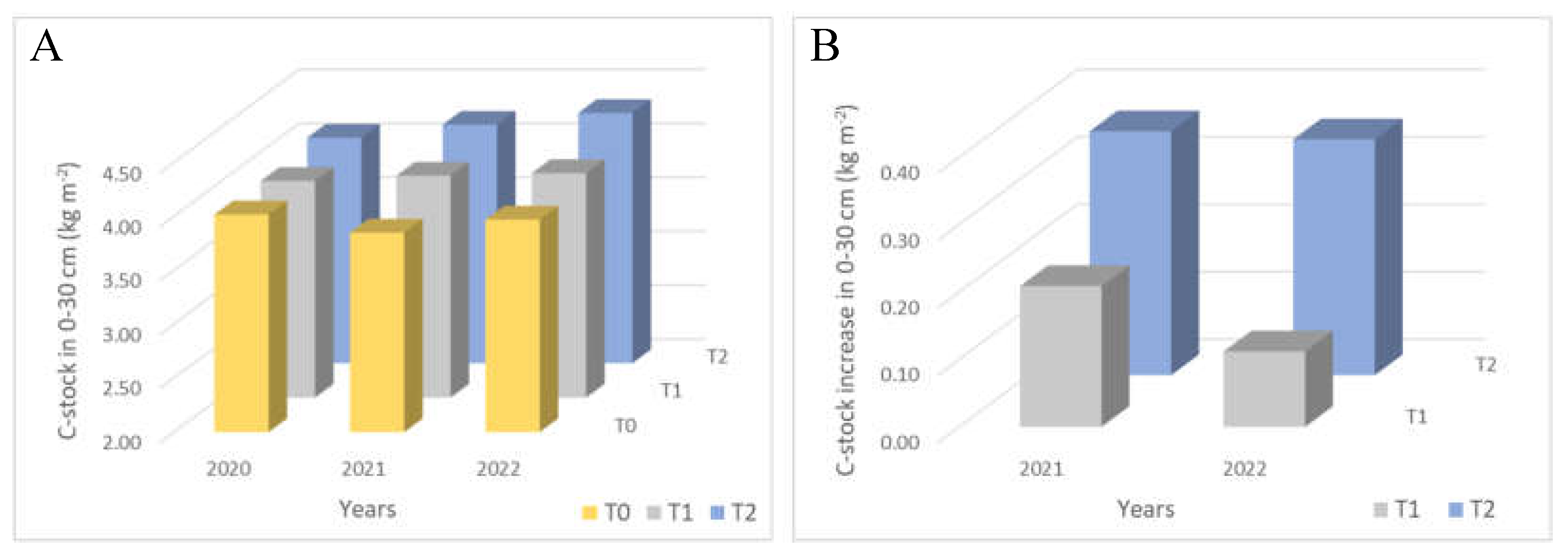
Although the soil C-stock depends not only on SOC but also on the rock fragments and the bulk density of the fine fraction (<2 mm), it followed, quite closely, the variation pattern of the SOC. There were no significant differences one year after the soil amendment (2021), and in the second year (2022) the differences were statistically significant only in the 5-15 cm depth layer, with treatment T2 having a significant higher C-stock than T1 and T0. In spite of the higher SOC of the upper layers, C-stock increase from the upper to the lower layer is due to layers thickness increase (from 5 to 15 cm in the same sequence) which overcomes the respective SOC decrease. Adding up C-stock mean values for each layer (Table 5) we get values for layer 0-30 which varies from 3.85 kg m^-2 (T0, 2021) to 4.32 kg m^-2 (T2, 2022) (Figure 5A).

Figure 5. (A) mean C-stock (kg m^-2) in layer 0-30 cm with treatments T0 (control, 0 kg m^-2), T1 (2.5 kg m^-2), and T2 (5.0 kg m^-2); (B) mean C-stock added to layer 0-30 cm with T1 and T2, one year (2021), and two years (2022) after compost addition.

Figure 5. (A) mean C-stock (kg m^-2) in layer 0-30 cm with treatments T0 (control, 0 kg m^-2), T1 (2.5 kg m^-2), and T2 (5.0 kg m^-2); (B) mean C-stock added to layer 0-30 cm with T1 and T2, one year (2021), and two years (2022) after compost addition.

3.5. Total Nitrogen and C/N

Total nitrogen was determined only in soil samples collected one year after the amendment (2021, Table 6). Total N increase in T1 and T2 dosages is clear, and it has statistical significance for the first layer (0-5 cm). In the second layer (5-15 cm) there is also a slight increase, though not statistically significant, probably due to greater data dispersion of T1 and T2 results.

Data of the ratio C/N showed that the average values in T1 and T2 treatment are lower than in T0, especially in the first layer (0-5 cm) where the differences have a strong statistically meaning. However, T1 and T2 in this same layer, are not statistically different. Like the first layer, the 5-15 cm layer showed a C/N decrease in the sequence T0>T1>T2, but without statistically significant differences between the treatments. The C/N ratio of the 15-30 cm layer did not seem to be affected by the presence of the compost.

Table 6. Total nitrogen (N) and C/N ratio for T0 (0 kg m^-2), T1 (2.5 kg m^-2), and T2 (5.0 kg m^-2).

Layer	N (g kg-1)							C/N
(cm)	T0		T1		T2			T0		T1		T2
	m*	s*	m	s	m	s		m	s	m	s	m	s
	2021
00-05	1.1a	0.1	2.4b	0.3	2.8b	0.5		13.7a	0.4	7.2b	1.4	6.3b	1.2
05-15	0.9	0.2	1.2	0.3	1.4	0.4		12.8	1.1	11.0	2.7	10.0	2.2
15-30	0.7	0.0	0.7	0.2	0.8	0.1		12.4	1.5	12.8	3.7	11.9	1.0

* mean (m) and standard deviation (s) of three plots per treatment (one composite sample per plot). a, b… values with the same letter within a line have a P≤0.05 of being equal means.

Table 6. Total nitrogen (N) and C/N ratio for T0 (0 kg m^-2), T1 (2.5 kg m^-2), and T2 (5.0 kg m^-2).

Layer	N (g kg-1)							C/N
(cm)	T0		T1		T2			T0		T1		T2
	m*	s*	m	s	m	s		m	s	m	s	m	s
	2021
00-05	1.1a	0.1	2.4b	0.3	2.8b	0.5		13.7a	0.4	7.2b	1.4	6.3b	1.2
05-15	0.9	0.2	1.2	0.3	1.4	0.4		12.8	1.1	11.0	2.7	10.0	2.2
15-30	0.7	0.0	0.7	0.2	0.8	0.1		12.4	1.5	12.8	3.7	11.9	1.0

* mean (m) and standard deviation (s) of three plots per treatment (one composite sample per plot). a, b… values with the same letter within a line have a P≤0.05 of being equal means.

Analysis of the compost revealed a C/N (11.8) about 2 units lower than observed in the 0-5 cm layer of the soil. This difference would not easily explain the C/N decrease in the upper soil layers receiving organic amendment. We hypothesize that this C/N reduction is also due to the regular nitrogen fertilization of the olive grove, which could have induced higher microbiological activity and higher retention of nitrogen in the upper soil layers.

3.6. POM-C and POX-C

Before the soil amendment (2020), both the POM-C and the POX-C did not show significant differences between the plots allocated to the three levels of compost dosage, in all sampled soil layers (Table 7).

One year later (2021), differences in POM-C were very expressive in the first two layers (0-5 and 5-15 cm), both showing the same sequence of values (T0<T1<T2) with T1 and T2 showing statistically significant differences to T0, but not among themselves. These differences were attenuated in 2022 and, though meaningful, did not have statistical significance.

POM has intermediate dimensions (>0.53 mm) and is considered to represent an initial stage of potential C sequestration in soils [14].

Table 7. Carbon of the particulate organic matter (POM-C) and permanganate oxidizable carbon (POX-C) for treatments T0 (0 kg m^-2), T1 (2.5 kg m^-2), and T2 (5.0 kg m^-2).

Layer	POM-C (g kg-1)							POX-C (mg kg-1)
(cm)	T0		T1		T2			T0		T1		T2
	m*	s*	m	s	m	s		m	s	m	s	m	s
	2020
00-05	4.85	0.98	5.86	1.00	5.40	1.01		543	46	535	11	517	13
05-15	3.09	0.65	3.57	0.71	4.11	0.53		411	25	407	16	432	55
15-30	1.70	0.34	1.69	0.51	1.90	0.13		248	22	260	30	274	15
	2021
00-05	5.78a	0.33	9.33b	2.21	12.14b	1.39		547a	9	663a	85	771b	71
05-15	3.51a	0.86	5.14b	0.36	5.26b	0.53		380a	10	435a	47	470b	31
15-30	2.07	0.94	3.62	2.11	3.11	0.50		234a	14	255ab’	4	287b’	18
	2022
00-05	4.73	0.85	9.38	4.92	11.68	7.94		576a	37	659ab’	50	836b’	117
05-15	3.36	0.80	4.42	1.18	4.55	0.76		414a’	31	434a	23	492a’	38
15-30	2.46	1.51	3.47	2.00	1.81	0.15		248	45	254	37	265	82

* mean (m) and standard deviation (s) of three plots per treatment (one composite sample per plot). a, b… values with the same letter within a line have a P≤0.05 of being equal means, and with the same letter with an apostrophe (a’, b’…) have a P<0.10 of being equal means.

Table 7. Carbon of the particulate organic matter (POM-C) and permanganate oxidizable carbon (POX-C) for treatments T0 (0 kg m^-2), T1 (2.5 kg m^-2), and T2 (5.0 kg m^-2).

Layer	POM-C (g kg-1)							POX-C (mg kg-1)
(cm)	T0		T1		T2			T0		T1		T2
	m*	s*	m	s	m	s		m	s	m	s	m	s
	2020
00-05	4.85	0.98	5.86	1.00	5.40	1.01		543	46	535	11	517	13
05-15	3.09	0.65	3.57	0.71	4.11	0.53		411	25	407	16	432	55
15-30	1.70	0.34	1.69	0.51	1.90	0.13		248	22	260	30	274	15
	2021
00-05	5.78a	0.33	9.33b	2.21	12.14b	1.39		547a	9	663a	85	771b	71
05-15	3.51a	0.86	5.14b	0.36	5.26b	0.53		380a	10	435a	47	470b	31
15-30	2.07	0.94	3.62	2.11	3.11	0.50		234a	14	255ab’	4	287b’	18
	2022
00-05	4.73	0.85	9.38	4.92	11.68	7.94		576a	37	659ab’	50	836b’	117
05-15	3.36	0.80	4.42	1.18	4.55	0.76		414a’	31	434a	23	492a’	38
15-30	2.46	1.51	3.47	2.00	1.81	0.15		248	45	254	37	265	82

* mean (m) and standard deviation (s) of three plots per treatment (one composite sample per plot). a, b… values with the same letter within a line have a P≤0.05 of being equal means, and with the same letter with an apostrophe (a’, b’…) have a P<0.10 of being equal means.

POX-C showed a similar behaviour as POM-C in regard to treatments T0 and T2. However, the T1 treatment, though having intermediate values between T0 and T2, in all layers, neither in 2021 nor in 2022 those values were distinct enough from T0 to have a statistically significant difference. On the other hand, the effect of the compost on the soil POX-C, extended to the 15-30 cm layer in 2021, and to the 5-15 cm layer in 2022.

3.7. pH_H2O and pH_KCl

The soil pH_H2O did not show any significant difference between the treatments even two years after the soil amendment (Table 8). Only the pH_KCl showed a statistically significant higher value with both compost dosages (T1 and T2) in the 0-5 cm layer, after two years (2022). In addition to this, pH_KCl results revealed, more clearly than pH_H2O, an inversion of the sequence with depth, from layer 0-5 cm to layer 15-30 cm, both one and two years after the compost addition, and especially with the T2 treatment. While in 2020 the pH_KCl was higher (or approximately constant) in the lower layers, in 2021, and even more in 2022, there was an evident decrease of pH_KCl from the 0-5 to the 15-30 cm layer.

Table 8. Soil pH measured in a water suspension (1:2.5) and soil pH measured in a suspension with 1N KCl solution (1:2.5) for treatments T0 (0 kg m^-2), T1 (2.5 kg m^-2), and T2 (5.0 kg m^-2).

Layer	pHH2O							pHKCl
(cm)	T0		T1		T2			T0		T1		T2
	m*	s*	m	s	m	s		m	s	m	s	m	s
	2020
00-05	7.34	0.43	7.28	0.27	7.19	0.24		6.87	0.50	6.78	0.29	6.61	0.47
05-15	7.38	0.42	7.47	0.29	7.35	0.48		6.76	0.48	6.94	0.35	6.82	0.59
15-30	7.59	0.46	7.72	0.25	7.72	0.39		6.78	0.52	6.98	0.32	7.01	0.50
	2021
00-05	7.28	0.35	7.39	0.24	7.36	0.10		6.66	0.27	6.85	0.14	6.91	0.18
05-15	7.30	0.31	7.51	0.07	7.23	0.07		6.66	0.27	6.82	0.12	6.78	0.32
15-30	7.40	0.59	7.45	0.49	7.55	0.27		6.44	0.41	6.84	0.33	6.66	0.45
	2022
00-05	7.44	0.48	7.75	0.18	7.52	0.13		6.62a	0.21	7.15b	0.09	7.08b	0.09
05-15	7.54	0.55	7.80	0.23	7.40	0.14		6.64a’	0.22	7.12a’	0.23	6.78a	0.18
15-30	7.60	0.55	7.72	0.22	7.31	0.17		6.68	0.48	6.95	0.21	6.44	0.25

* mean (m) and standard deviation (s) of three plots per treatment (one composite sample per plot). a, b… values with the same letter within a line have a P≤0.05 of being equal means, and with the same letter with an apostrophe (a’, b’…) have a P<0.10 of being equal means.

Table 8. Soil pH measured in a water suspension (1:2.5) and soil pH measured in a suspension with 1N KCl solution (1:2.5) for treatments T0 (0 kg m^-2), T1 (2.5 kg m^-2), and T2 (5.0 kg m^-2).

Layer	pHH2O							pHKCl
(cm)	T0		T1		T2			T0		T1		T2
	m*	s*	m	s	m	s		m	s	m	s	m	s
	2020
00-05	7.34	0.43	7.28	0.27	7.19	0.24		6.87	0.50	6.78	0.29	6.61	0.47
05-15	7.38	0.42	7.47	0.29	7.35	0.48		6.76	0.48	6.94	0.35	6.82	0.59
15-30	7.59	0.46	7.72	0.25	7.72	0.39		6.78	0.52	6.98	0.32	7.01	0.50
	2021
00-05	7.28	0.35	7.39	0.24	7.36	0.10		6.66	0.27	6.85	0.14	6.91	0.18
05-15	7.30	0.31	7.51	0.07	7.23	0.07		6.66	0.27	6.82	0.12	6.78	0.32
15-30	7.40	0.59	7.45	0.49	7.55	0.27		6.44	0.41	6.84	0.33	6.66	0.45
	2022
00-05	7.44	0.48	7.75	0.18	7.52	0.13		6.62a	0.21	7.15b	0.09	7.08b	0.09
05-15	7.54	0.55	7.80	0.23	7.40	0.14		6.64a’	0.22	7.12a’	0.23	6.78a	0.18
15-30	7.60	0.55	7.72	0.22	7.31	0.17		6.68	0.48	6.95	0.21	6.44	0.25

* mean (m) and standard deviation (s) of three plots per treatment (one composite sample per plot). a, b… values with the same letter within a line have a P≤0.05 of being equal means, and with the same letter with an apostrophe (a’, b’…) have a P<0.10 of being equal means.

3.8. Macronutrients Phosphorus and Potassium

Macronutrients P and K showed a contrasting pattern (Table 9). While K did not reveal any statistically significant difference between treatments up to 30 cm depth, neither one year (2021) nor two years (2022) after the compost spreading, there were some significant differences of P in both years, mainly in the most superficial layer (0-5 cm).

Table 9. Phosphorus (expressed as P₂O₅) and potassium (expressed as K₂O) for treatments T0 (0 kg m^-2), T1 (2.5 kg m^-2), and T2 (5.0 kg m^-2).

Layer	P2O5 (mg kg-1)							K2O (mg kg-1)
(cm)	T0		T1		T2			T0		T1		T2
	m*	s*	m	s	m	s		m	s	m	s	m	s
	2020
00-05	160.7	47.3	163.0	24.9	123.4	45.2		390	114	407	78	363	58
05-15	103.3	24.6	105.8	4.3	83.4	25.9		330	89	310	40	287	12
15-30	40.0	8.7	46.5	7.4	35.5	8.7		227	56	230	44	207	12
	2021
00-05	185.7a	70.2	395.3b	52.3	550.7c	28.7		532	154	508	179	700	21
05-15	115.3a’	42.3	188.7a	32.9	223.0a’	71.0		296	122	338	71	321	120
15-30	48.7	16.2	73.0	9.8	87.7	38.7		193	44	226	36	180	16
	2022
00-05	227.3a	66.5	373.7b	45.6	434.3b	60.2		311	156	355	110	343	115
05-15	105.7	26.5	153.0	30.8	142.3	22.7		158	58	191	52	209	31
15-30	33.0	14.1	32.3	8.1	32.3	5.5		133	37	135	46	126	17

* mean (m) and standard deviation (s) of three plots per treatment (one composite sample per plot). a, b… values with the same letter within a line have a P≤0.05 of being equal means, and with the same letter with an apostrophe (a’, b’…) have a P<0.10 of being equal means.

Table 9. Phosphorus (expressed as P₂O₅) and potassium (expressed as K₂O) for treatments T0 (0 kg m^-2), T1 (2.5 kg m^-2), and T2 (5.0 kg m^-2).

Layer	P2O5 (mg kg-1)							K2O (mg kg-1)
(cm)	T0		T1		T2			T0		T1		T2
	m*	s*	m	s	m	s		m	s	m	s	m	s
	2020
00-05	160.7	47.3	163.0	24.9	123.4	45.2		390	114	407	78	363	58
05-15	103.3	24.6	105.8	4.3	83.4	25.9		330	89	310	40	287	12
15-30	40.0	8.7	46.5	7.4	35.5	8.7		227	56	230	44	207	12
	2021
00-05	185.7a	70.2	395.3b	52.3	550.7c	28.7		532	154	508	179	700	21
05-15	115.3a’	42.3	188.7a	32.9	223.0a’	71.0		296	122	338	71	321	120
15-30	48.7	16.2	73.0	9.8	87.7	38.7		193	44	226	36	180	16
	2022
00-05	227.3a	66.5	373.7b	45.6	434.3b	60.2		311	156	355	110	343	115
05-15	105.7	26.5	153.0	30.8	142.3	22.7		158	58	191	52	209	31
15-30	33.0	14.1	32.3	8.1	32.3	5.5		133	37	135	46	126	17

* mean (m) and standard deviation (s) of three plots per treatment (one composite sample per plot). a, b… values with the same letter within a line have a P≤0.05 of being equal means, and with the same letter with an apostrophe (a’, b’…) have a P<0.10 of being equal means.

The compost tested has significant levels of phosphorous (5.1 g kg^-1 P₂O₅) and potassium (6.1 g kg^-1 K₂O). The levels of phosphorous and the low mobility of this macronutrient can explain its observed increase, mainly in the upper layer, just up to 5 cm deep. On the other hand, the main reason why the similarly levels of potassium provided by the compost do not stand out so much as the phosphorous, could be the three times higher content in potassium of the fertilizer regularly use in this olive grove (4% P₂O₅ to 12% K₂O).

3.9. Micronutrients Cations (Fe, Mn, Cu and Zn)

As for micronutrients, only soil samples collected one year (2021) and two years (2022) after compost addition were analyzed (Table 10 and Table 11).

Extractable Fe does not register significant changes in any of the three layers in neither of the two years monitored (Table 10).

Mn tends to decrease with the compost addition, but only moderately significant differences (P<0.10) were verified two years (2022) after the application and up to 15 cm deep (Table 10). This slight decrease in extractable Mn in the upper soil layers can be associated with the observed pH_H2O and pH_KCl increase in these layers (Table 8), and the resulting Mn solubility reduction.

Table 10. Micronutrients Fe and Mn for treatments T0 (0 kg m^-2), T1 (2.5 kg m^-2), and T2 (5.0 kg m^-2).

Layer	Fe (mg kg-1)							Mn (mg kg-1)
(cm)	T0		T1		T2			T0		T1		T2
	m*	s*	m	s	m	s		m	s	m	s	m	s
	2021
00-05	156	65	205	41	236	29		405	102	369	29	299	49
05-15	144	69	162	18	154	31		390	87	399	32	312	46
15-30	139	65	165	53	102	30		342	110	357	110	236	66
	2022
00-05	134	36	162	32	200	29		357a’	43	351a	43	278a’	27
05-15	112	18	127	35	117	7		340a	25	357a’	28	297a’	27
15-30	169	102	141	79	116	32		284	17	321	53	319	50

* mean (m) and standard deviation (s) of three plots per treatment (one composite sample per plot). a, b… values with the same letter within a line have a P≤0.05 of being equal means, and with the same letter with an apostrophe (a’, b’…) have a P<0.10 of being equal means.

Table 10. Micronutrients Fe and Mn for treatments T0 (0 kg m^-2), T1 (2.5 kg m^-2), and T2 (5.0 kg m^-2).

Layer	Fe (mg kg-1)							Mn (mg kg-1)
(cm)	T0		T1		T2			T0		T1		T2
	m*	s*	m	s	m	s		m	s	m	s	m	s
	2021
00-05	156	65	205	41	236	29		405	102	369	29	299	49
05-15	144	69	162	18	154	31		390	87	399	32	312	46
15-30	139	65	165	53	102	30		342	110	357	110	236	66
	2022
00-05	134	36	162	32	200	29		357a’	43	351a	43	278a’	27
05-15	112	18	127	35	117	7		340a	25	357a’	28	297a’	27
15-30	169	102	141	79	116	32		284	17	321	53	319	50

* mean (m) and standard deviation (s) of three plots per treatment (one composite sample per plot). a, b… values with the same letter within a line have a P≤0.05 of being equal means, and with the same letter with an apostrophe (a’, b’…) have a P<0.10 of being equal means.

Extractable Cu and Zn, both increased with the compost treatments, but there are some differences among them (Table 11). While Cu increase was more evident only two years after the compost application (2022), and was just moderately significant in the first two layers (P<0.10), Zn was the most affected micronutrient, showing significant increases with both compost dosages (T1 and T2) and in both years. Despite the strong signals given by the Zn, especially after the first year, a great variability of values occurred in the 5-15 cm layer which prevented the statistical significance of the differences observed in this layer. Additionally, the extractable Zn was substantially reduced in the second year, but the differences between T2 and T0 showed statistical significance up to 15 cm depth.

Table 11. Micronutrients Cu and Zn for treatments T0 (0 kg m^-2), T1 (2.5 kg m^-2), and T2 (5.0 kg m^-2).

Layer	Cu (mg kg-1)							Zn (mg kg-1)
(cm)	T0		T1		T2			T0		T1		T2
	m*	s*	m	s	m	s		m	s	m	s	m	s
	2021
00-05	47.0	8.3	56.8	13.6	57.7	8.3		5.6a	5.2	44.2b’	9.5	58.3b’	3.8
05-15	29.0	6.5	39.5	14.3	30.8	5.7		1.8	0.4	14.4	13.5	20.7	18.9
15-30	13.5	1.4	14.9	3.3	13.6	5.0		1.3a	0.1	4.3b	1.0	5.2b	0.5
	2022
00-05	47.0a’	6.0	58.3a	8.5	63.7a’	7.6		2.7a	0.6	17.0b	4.0	27.0b	8.2
05-15	28.3a’	6.7	40.0a’	3.0	33.0a	3.5		1.7a	0.6	2.7ab	0.6	4.0b	1.0
15-30	6.3a	1.2	9.7ab	2.1	14.7b	4.7		1.0	0.0	1.3	0.6	1.7	0.6

* mean (m) and standard deviation (s) of three plots per treatment (one composite sample per plot). a, b… values with the same letter within a line have a P≤0.05 of being equal means, and with the same letter with an apostrophe (a’, b’…) have a P<0.10 of being equal means.

Table 11. Micronutrients Cu and Zn for treatments T0 (0 kg m^-2), T1 (2.5 kg m^-2), and T2 (5.0 kg m^-2).

Layer	Cu (mg kg-1)							Zn (mg kg-1)
(cm)	T0		T1		T2			T0		T1		T2
	m*	s*	m	s	m	s		m	s	m	s	m	s
	2021
00-05	47.0	8.3	56.8	13.6	57.7	8.3		5.6a	5.2	44.2b’	9.5	58.3b’	3.8
05-15	29.0	6.5	39.5	14.3	30.8	5.7		1.8	0.4	14.4	13.5	20.7	18.9
15-30	13.5	1.4	14.9	3.3	13.6	5.0		1.3a	0.1	4.3b	1.0	5.2b	0.5
	2022
00-05	47.0a’	6.0	58.3a	8.5	63.7a’	7.6		2.7a	0.6	17.0b	4.0	27.0b	8.2
05-15	28.3a’	6.7	40.0a’	3.0	33.0a	3.5		1.7a	0.6	2.7ab	0.6	4.0b	1.0
15-30	6.3a	1.2	9.7ab	2.1	14.7b	4.7		1.0	0.0	1.3	0.6	1.7	0.6

* mean (m) and standard deviation (s) of three plots per treatment (one composite sample per plot). a, b… values with the same letter within a line have a P≤0.05 of being equal means, and with the same letter with an apostrophe (a’, b’…) have a P<0.10 of being equal means.

4. Discussion

SOC and total N significant increase are common effects on soil as result of the application of different composts [2,5,7]. The results obtained in this study are aligned with that trend, though the high variability of the SOC in the first year (2021), especially in the first two layers, has prevented statistically significant differences between the treatments. This could be also a consequence of the spreading at soil surface, when compared to the alternative solution of incorporating the organic amendment in a given superficial soil layer. It is worth to emphasize that the results of the previous mentioned studies were obtained after three, five, or more years. In the second year of this study, trends of increasing SOC and some statistically significant differences for T1 and T2 were already obtained. It is expected that the compost spreading at soil surface, though having a slower effect on SOC content, could prevent the unavoidable SOC loss due to soil mobilization for compost incorporation.

The effect of the compost on the mean C-stock of layer 0-30 cm deep (Figure 5B) was 0.21 and 0.36 kg m^-2 for T1 and T2 in 2021, and 0.11 and 0.35 kg m^-2 for T1 and T2 in 2022. From 2021 to 2022, T1 suffered a stronger decrease of the C-stock than T2, for no apparent reason, unless the fact that the lower C-stock increase in T1 is more affected by some data variability, not only in T1 plots but also in the control plots. These results recommend longer periods of time for C-stock monitoring. However, based on the C applied with the compost (~0,23 and ~0,66 kg m^-2, for T1 and T2 dosages, respectively) at the end of the second year, both treatments reveal approximately 50% of C incorporation in the soil.

POX-C is assumed to reflect management practices that promote organic matter accumulation or stabilization, being considered a useful indicator of long-term soil C sequestration [21]. POX-C was the most sensitive indicator revealing increases up to 30 cm deep after one year. Although the POX-C should still be monitored for longer periods of time, the results obtained in the first two years seem to confirm the interest of this analytical parameter to detect effects of agricultural practices on soil organic matter [22].

It seems that pH_KCl could be a better indicator of the soil pH changes induced by the compost. Although the non-acid cations (mainly Ca and Mg) added by the compost could have contributed to increase pH in the upper soil layers, the parallel increment of the biological activity near soil surface, namely due to nitrogen increase (Table 6), could contribute to pH reduction with depth.

Macro and micronutrients increase, namely in P, Cu and Zn are concomitant with results obtained by other studies with different composts and after longer periods of time [2,5].

The proportionally small increase in Cu with T1 and T2 relatively to the control (T0) can be explained by the olive leaves component. The regular use of Cu-based phytopharmaceuticals (namely copper oxy-sulphide, personal communic.) in this olive grove must be also reflected in the soil of the control plots (T0), especially in the row, under the tree canopy.

Based on the Zn content of the compost (219 mg kg^-1) its total incorporation in the 0-5 cm soil layer would give an increase in soil Zn content of ~7 and ~20 mg kg^-1, for T1 and T2 dosages, respectively, much lower values than the ~40 mg kg^-1, and ~50 mg kg^-1 increase observed in the same treatments. It is well known that Zn solubility increases with organic complexes, especially near neutral or slightly alkaline soil pH as the soil of this study. Additionally, at pH 7, more stable Zn complexes are formed with humic acids of weakly humified structures [23], which could explain the reduction on the extractable Zn observed in the second year, both by progressive Zn leaching and reduction of stable complexes, i.e., due to mineralization and evolution to more humified structures.

The studied compost reveled potential to increase soil C-stock, and to improve soil quality and soil fertility, and its use can be considered as a sustainable soil management practice. Nevertheless, its effects should be monitored over longer periods of time, namely on SOC and extractable zinc.

References

- Pergola, M.; Persiani, A.; Palese, A.M.; Di Meo, V.; Pastore, V.; D’Adamo, C.; Celano, G. Composting: The Way for a Sustainable Agriculture. Applied Soil Ecology 2018, 123, 744–750. [Google Scholar] [CrossRef]
- Brown, S.; Cotton, M. Changes in Soil Properties and Carbon Content Following Compost Application: Results of On-Farm Sampling. Compost Science & Utilization 2011, 19, 87–96. [Google Scholar] [CrossRef]
- Wang, D.; Lin, J.Y.; Sayre, J.M.; Schmidt, R.; Fonte, S.J.; Rodrigues, J.L.M.; Scow, K.M. Compost Amendment Maintains Soil Structure and Carbon Storage by Increasing Available Carbon and Microbial Biomass in Agricultural Soil – A Six-Year Field Study. Geoderma 2022, 427, 116117. [Google Scholar] [CrossRef]
- Rodríguez Sousa, A.A.; Muñoz-Rojas, J.; Pinto-Correia, T.; Aguilera, P.A.; Barandica, J.M.; Rescia, A.J. A Comparative Analysis of Soil Loss Tolerance and Productivity of the Olive Groves in the Protected Designation of Origin (PDO) Areas Norte Alentejano (Portugal) and Estepa (Andalusia, Spain). Agronomy 2021, 11, 665. [Google Scholar] [CrossRef]
- Chehab, H.; Tekaya, M.; Ouhibi, M.; Gouiaa, M.; Zakhama, H.; Mahjoub, Z.; Laamari, S.; Sfina, H.; Chihaoui, B.; Boujnah, D.; et al. Effects of Compost, Olive Mill Wastewater and Legume Cover Crops on Soil Characteristics, Tree Performance and Oil Quality of Olive Trees Cv.Chemlali Grown under Organic Farming System. Scientia Horticulturae. 2019, 253, 163–171. [Google Scholar] [CrossRef]
- García-Ruiz, R.; Ochoa, M.V.; Hinojosa, M.B.; Gómez-Muñoz, B. Improved Soil Quality after 16 Years of Olive Mill Pomace Application in Olive Oil Groves. Agron. Sustain. Dev. 2012, 32, 803–810. [Google Scholar] [CrossRef]
- Chaker, R.; Gargouri, K.; Ben Mbarek, H.; Maktouf, S.; Palese, A.M.; Celani, G.; Bouzid, J. Carbon and Nitrogen Balances and CO2 Emission after Exogenous Organic Matter Application in Arid Soil. Carbon Management 2019, 10, 23–36. [Google Scholar] [CrossRef]
- IPMA. Normal Climatológica – Portalegre (1981-2010). Instituto Português do Mar e da Atmosfera, I. P., 2022; pp. 3. https://www.ipma.pt/bin/file.data/climate-normal/cn_81-10_PORTALEGRE.pdf (accessed on 7 March 2023).
- IPMA. Boletim Climatológico Sazonal. Instituto Português do Mar e da Atmosfera, I. P., 2020-2022. pp. 7. https://www.ipma.pt/pt/publicacoes/boletins.jsp?cmbDep=cli&cmbTema=pcl&idDep=cli&idTema=pcl&curAno=-1 (accessed on 7 March 2023).
- SROA. Carta dos Solos de Portugal (Esc. 1:50.000). Secretaria de Estado da Agricultura. Lisboa, 1970. 162 pp.
- Sempiterno, C., Fernandes, R., Peça, J., Dias, A., Pinheiro, A., Saragoça, J., Pedra, F. Valorização agrícola de subprodutos do olival e do lagar – GO TECOLIVE. In: Livro de Resumos IX Simpósio Nacional de Olivicultura; Ramos, A. C., Pereira, J. A. and Rodrigues, N., Eds.; Associação Portuguesa de Horticultura (APH), Oeiras, Portugal, 2021; pp. 153–162.
- Blake, G.R.; Hartge, K.H. Bulk Density. In Methods of Soil Analysis; John Wiley & Sons, Ltd, 1986; pp. 363–375 ISBN 978-0-89118-864-3.
- Poeplau, C.; Vos, C.; Don, A. Soil Organic Carbon Stocks Are Systematically Overestimated by Misuse of the Parameters Bulk Density and Rock Fragment Content. SOIL 2017, 3, 61–66. [Google Scholar] [CrossRef]
- Cambardella, C.A.; Elliott, E.T. Particulate Soil Organic-Matter Changes across a Grassland Cultivation Sequence. Soil Science Society of America Journal 1992, 56, 777–783. [Google Scholar] [CrossRef]
- Soil Survey Staff. Kellogg Soil Survey Laboratory Methods Manual. Soil Survey Investigations Report No. 42, Version 5.0. R. Burt and Soil Survey Staff (ed.). U.S. Department of Agriculture, Natural Resources Conservation Service. 2014.
- Weil, R.R.; Islam, K.R.; Stine, M.A.; Gruver, J.B.; Samson-Liebig, S.E. Estimating Active Carbon for Soil Quality Assessment: A Simplified Method for Laboratory and Field Use. American Journal of Alternative Agriculture 2003, 18, 3. [Google Scholar] [CrossRef]
- Culman, S.; Freeman, M.; Snapp, S. (2014). Procedure for the Determination of Permanganate Oxidizable Carbon. Mich-igan State University. East Lansing, Michigan. USA. https://lter.kbs.msu.edu/protocols/133 (accessed on 3 November 2022).
- Egnér, H.; Riehm, H.; Domingo, W.R. Untersuchungen uber die chemische Bodenanalyse als Grundlage fur die Beurteilung des Nährstoffzustandes der Böden. II. Chemische Extraktionsmethoden zur Phosphor- und Kaliumbestimmung. Kungliga Lantbrukshögskolans Annaler. 1960, 26, 199–215.
- Lakanen, E.; Erviö, R. A Comparison of Eight Extractants for the Determination of Plant Available Micronutrients in Soils. Acta Agr Fenn 1971, 123, 223–232. [Google Scholar]
- R Core Team: The R Project for Statistical Computing. Available online: https://www.r-project.org/ (accessed on 22 June 2023).
- Hurisso, T.T.; Culman, S.W.; Horwath, W.R.; Wade, J.; Cass, D.; Beniston, J.W.; Bowles, T.M.; Grandy, A.S.; Franzluebbers, A.J.; Schipanski, M.E.; et al. Comparison of Permanganate-Oxidizable Carbon and Mineralizable Carbon for Assessment of Organic Matter Stabilization and Mineralization. Soil Science Society of America Journal 2016, 80, 1352–1364. [Google Scholar] [CrossRef]
- Lucas, S.; Weil, R. Can Permanganate Oxidizable Carbon Predict Soil Function Responses to Soil Organic Matter Management? Soil Science Society of America Journal 2021, 85, 1768–1784. [Google Scholar] [CrossRef]
- Boguta, P.; Sokołowska, Z. Interactions of Zn(II) Ions with Humic Acids Isolated from Various Type of Soils. Effect of pH, Zn Concentrations and Humic Acids Chemical Properties. PLoS ONE, 2016, 11(4): 1-20. [CrossRef]
Disclaimer/Publisher’s Note: The statements, opinions and data contained in all publications are solely those of the individual author(s) and contributor(s) and not of MDPI and/or the editor(s). MDPI and/or the editor(s) disclaim responsibility for any injury to people or property resulting from any ideas, methods, instructions or products referred to in the content. |
© 2023 by the authors. Licensee MDPI, Basel, Switzerland. This article is an open access article distributed under the terms and conditions of the Creative Commons Attribution (CC BY) license (http://creativecommons.org/licenses/by/4.0/).
Copyright: This open access article is published under a Creative Commons CC BY 4.0 license, which permit the free download, distribution, and reuse, provided that the author and preprint are cited in any reuse.