
Submitted:
21 June 2023
Posted:
25 June 2023
You are already at the latest version
Abstract
Macrophytes and seagrasses play a crucial role with a variety of the functions in the marine ecosystem and respond synchronized-promptly to the changing climate, followed by ecological status. Monitoring of the seagrasses was one of the paramount topics at the marine environment. One of the fast monitoring techniques is the vegetation acoustics with the advantages compared to the other remote sensing techniques. The acoustic method alone is ambitious to sea-truth identities of the backscatterers at the sea. Therefore, a package of computer programs was developed to identify, estimate leaf biometrics (leaf length and biomass) of one of the common seagrasses, Posidonia oceanica. Some troubleshooting in the acoustical data were fixed and then solved to reach the estimates regarding to the matters encountered for the vegetation as well as fisheries and plankton acoustics. One of the trouble was the “Lost” bottom which occurred during the data collection and post-processing due to occurrence of the acoustical noises, reverberations, interferences and intense scatterers suchlike fish schools. Another problem to remove was the occurrence as studying the near-bottom echoes belonging to submerged vegetations such as seagrasses, followed by spurious echoes. Last one was recognition of the seagrass to estimate leaf length and biomass calibrating the sheaths/vertical rhizome of the seagrass and establishing relationships between acoustical units and biometrics, respectively. As a consequence, an autonomous package of the code written in language MatLab was developed to perform all processes, and the name of the package was abbreviated as POSIBIOM, POSIdonia BIOMass. This study presented the algorithms, methodology, acoustics-biometrics relation, and mapping of the biometrics for the first time, and discussed advantages and disadvantages of the package compared to the software purposed for the bottom types, habitat and vegetation acoustic. The future studies were recommended to improve the package.
Keywords:
acoustics
; seagrass
; computer programs
; sea-truthing
; estimates
; leaf
; biomass
1. Introduction
Aquatic macrophyt (algae, grass etc) is one of the
important components playing a crucial role in various ways for the aquatic
ecosystem [1–3]. Considering the volume and
surface area of the marine system, seaweeds and seagrass have significant
contribution primarily with their oxygen production and carbon
absorbance/emission into a way of the ocean-atmosphere interaction. Besides
microscopic algae and photosynthetic bacteria, most of marine macrophytes
reveal status of the marine ecosystem health and ecological
level. Some of them are indicators of pollution whereas some are indicators of
the pristine environment [4,5]. There are a lot of further importance and contributions
of them to the marine system. Unlike the algae, the seagrasses are associated
with the sediments (benthic system) by their below-ground parts (rhizomes, and
roots) [6] and pelagic system by their above-ground parts (sheaths,
and leaves) [5].
One of the common seagrasses, Posidonia
species, the phanerogam species which have been sustained well in the
poor-nutrient marine environment and formed colonial life are coastal species,
and are worldwide distributed in the subtropical and temperate waters from
Indo-Pacific Ocean (Australia) to Atlantic Ocean (Mediterranean Sea) systems [7,8]. They are very sensitive to the pollution,
climate change, global warming, biogeochemical cycle, anthropogenic effects and
water movements etc [9–11]. Their biometrical
traits respond rapidly to such global or local events in order for the
scientists to monitor health of the marine system. Like other seagrasses, Posidonia
species are near coastal inhabitants giving many useful opportunities to the
other organisms under their canopies [4,12–15].
One of the common Posidonia species is Posidonia oceanica (Linnaeus)
Delile, 1813 which is an endemic species for the Mediterranean Sea extending to
near coast of the eastern Atlantic Ocean [16].
Most (25-30%) of the Mediterranean coasts are inhabited by P. oceanica [6].
Like other seagrass (angiosperms), Posidonia
oceanica (the Mediterranean meadow) is a prominent component in the zonal
classification in the Mediterranean Sea, and classifies the border between the
Infralittoral and the Circalittoral of the benthic environment [1,3,5,17,18]. Therefore, it is positioned as a
coastal engineer and interior architect in the coastal environment with their
following functions [19,20]. Besides the
ecological indication, Posidonia oceanica also play crucial roles in the
sediment stability and biogeochemical cycle, oxygen, carbon
emission/absorbance, blue carbon, habitat/shelter and food niches for its
interacted organisms, spawning and nursery grounds, competition with invasive
macrophytes, protectors of prey from predator, and extension of their habitants
in range [14,21–30]. Monitoring their dynamics
is a useful tool to sustain the species under the prevailing environment, and
to observe indicative acute or chronic changes derived from the allochthonous
and autochthonous sources in the marine ecosystem. Consequently, this knowledge
is used by the ecosystem modelers, ecologists, environmentalist, biologists,
coastal engineers and managers, and species managers and protectors [31–33].
Compared to fish and zooplankton acoustics,
vegetations acoustics have not however attracted significant attention of
researchers. The destructive sampling methods (SCUBA sampling to pick up the
seagrass) are not generally desired to sample the meadow under the protection [34–36]. Therefore, many studies were fronted to
apply non-destructive methods, remote sensing systems to study sensitive and
vulnerable seaweeds and seagrass [37]. There
are a variety of remote sensing techniques developed as follows: satellites
(especially Sentinel 2), video cameras and acoustics [38–44].
There are some limitations to sample the seagrass significantly for each
technique. Visual techniques (satellite, and video-camera) are limited with
requirements of the suitable atmospheric and sea conditions [45–47]. These techniques were mostly used for the
estimates of coverage and mapping of the different habitats e.g., [48,49]. Compared to the techniques, the acoustical
method is faster, more precise, and easier and does not need clear sea
conditions to sample the data [2,50], and but
have serious problems changing from correct bottom detection, removal of
spurious scatterers to sea-truthing of the targets [51].
Recently, in/ex situ acoustical studies have increased to relate
the biometrics of the seaweeds and seagrasses to the Elementary Distance
Sampling Unit (EDSU) [52], for instance, Depew
et al. [53] focused on Cladophora sp., Monpert
et al. [54] on P. oceanica, and Zostera
marina, Llorens-Escrich et al. [55] on P.
oceanica, Shao et al. [56] on Saccharina
japonica, and Minami et al. [57] on Sargassum
horneri. There were some studies to calibrate the acoustical data versus
the biometrics of two seagrasses, P. oceanica and Cymodocea nodosa
[58–61] and to identify the seagrass, P.
oceanica and C. nodosa [62].
Like that in the other remote sensing techniques,
acoustic data alone are inherently ambiguous with regard needed to the
identities of the target species. The mapping of macrophytes can be
accomplished with the software developed for the submerged vegetation
(EcoSAV:Echo Submerged Aquatic Vegetation, Visual Habitat and Visual Aquatic)
by BioSonics Company. Further methods of vegetation acoustics were developed
based on algorithms to classify bottom types [63–66].
They are OTCView, Echoplus, BioSonics VBT (Visual Bottom Typer), and EchoView [67–70]. While the acoustic reflectivity of aquatic
vegetation having an acoustical impedance of 1.026 to seawater [71] is known and used for the detection of
submerged aquatic vegetation (SAV) [72], the
basis of this phenomenon has not yet been figured out to solve the problems.
The other detection factor is the acoustical frequency used during the
vegetation acoustical studies. Although the most effective frequency for these
techniques is 420 kHz, it has been concluded that 200 kHz is also effective for
vegetation acoustics [73].
The present study is aimed to solve the problems,
detect and discriminate the Mediterranean meadow, and estimate the leaf biomass
for the future works and studies needing the biomass purposed by the researches
for sustaining the meadow. The presence of life on the sea bed causes
significant problems during acoustic post-processing, including spurious
targets, background noise, artificially generated-noise, reverberations, dead
zones, interference, ‘lost’ bottoms (misestimated bottom, too deep, out of
range of sound penetration by the frequency limitation depending on the source
level). In particular, the problem of ‘lost’ bottoms in stock assessments of
the species creates challenges when attempting to recover bottom echoes. In
some cases, commercial software and computer scripts require interventions to
manually recover ‘lost’ bottoms, which could be time-consuming. This study is
the first attempt to regard the matters of the acoustical data post-processing
aimed to estimate biometrics of P. oceanica, and presents an auto-self
(no often intervention) and easy used-package of the scripts codes to solve the
problems during the estimation with advantages and disadvantages of the codes
in comparison to the other software.
2. Material and Methods
Overall, acoustical raw data (*.dt4) used for the
present study were collected with a Biosonics DT-X
digital scientific echosounder which had a split beam transducer in a shape
of circle beaming a width (θ) of 6.8°,
operating 206 kHz using a software package of “Visual Acquisition” (v.
6.3.1.10980, BioSonics inc.). The pulse width (pulse length, pulse duration, τ) was set to 0.1 ms (highly recommended for
the seagrass studies), a ship speed to approximately no more than 5 knots, and
no deeper bottom than 50-60 m. The transducer was
mounted at a draft depth of 2.5 m down-looking on the starboard of the R/V Akdeniz Su [74,75]). During the
surveys of different sampling locations and months, different bottom types
covered by the seagrass were encountered namely, rock, sand, mud and matte [5,18].
Three main script codes which run autonomously after all settings completed by the users were written in MatLab (vers. 2021a, Matworks inc.) to correct the bottom depth, to remove spurious weak and strong scatterers else than Posidonica oceanica and to sort out the species regarding to its vertical rhizome and sheath. To recover removal of the debugs in the package, around 4000 acoustical files (300-9000 pings, 4500 pings per file on average) derived from two different projects [74,75] were subjected to the codes. Three main codes subsequently run as follows: “AbdezdeR1”, “AbemsiR1” and “SheathFinder1” to estimate ultimate data of the biomass (see Mutlu and Balaban [58] for the description of abbreviations of the algorithm names). There are several auxiliary scripts and acoustical data associated with the three main codes. All three codes run under a script as a main menu and manager to reach them. It is called in an acronomy of ‘POSIBIOM’ as abbreviation of POSIdonia BIOMass. The present study was inspired from an algorithm, ‘SheathFinder’ [58]. However, the algorithm was not a package, easy-used, and was debugged to estimate real bottom echo without infinitive permutation until all ‘lost’ bottoms completed disregarding seasonal biomass estimates of the seagrass. Therefore, all algorithms were highly revised and modified completely for the present study. In the present, the acoustical data collected only with only the BioSonics inc. echosounders can be used for the POSIBIOM since I am currently a user of BioSonics echosounder. To run the scripts, the data (*.dt4) was converted to a spread sheet of Comma-Separated Value (CSV) using a post-processing commercial program, “Visual Analyzers” (v. 4.1.2.42, Biosonics inc.). During the post-processing, the settings were configured to get output data in a vertical resolution of count-to-count (equivalent of ~one-eighth of the pulse width in cm depending on seasonal sound speed) and in a horizontal resolution of ping-to-ping. The processes were repeated to get the layered data including the seagrass from the uneven (not flat) bottom up to a stratum number of 249 (this is the last number allowed by the Visual Analyzer). This could be done once for the flat bottom to get count-to-count data of the vertical resolution. This is important to determine precise and accuracy of the vertical resolution of leaf length, hence biomass. This process is but time-consuming. It would be helpful and faster for processing the data if the scripts (POSIBIOM) read the collected data file of the BioSonics directly. In order for POSIBIOM to be professional software, the package would be coded to a programming language of the ‘C’ from the MatLab by its relevant tool.
The POSIBIOM is functioned as a manager to load input files (acoustical and coast line files, Marine Region [76]), to start each of three analyses, and to map the results of the biomass and leaf length of the seagrass (Appendix 1).
2.1. Algorithm of ‘lost’ bottom (AbdezdeR1)
The algorithm was scripted in a file, namely, AbdezdeR1 (see Mutlu and Balaban [58] for description of the abbreviation). Fixation of lost bottom is based on a root of adjacent bottom angles and depths. Configuration for recovery of real bottom is highly flexible during the processing. The fixed lost bottom is corrected with the following three successive methods, namely; the “chirping”, “running average” and “filling gap”. All methods were originated for the present study. The algorithm then estimates the dead zone using three methods. One method was created during the present study, and the other two methods have been described by EchoView [77] and Mello and Rose [78]. The algorithm has some options to alert users automatically in some cases to correct the bottom before the analyses (Appendix 2), and for last check of the bottom correction after the analyses (see Table 1, Figure 7). The algorithm is also useful for other purposes (e.g., fisheries acoustics, and partly plankton acoustics) else rather than the vegetation acoustics.
2.1.1. Real bottom recovery
Fixing misestimated bottom regards the sudden change of the bottom angle in successive pings. The angle to search the fake (second echo of the bottom, sheer of returned echo with the next pulse in the water column) bottom was followed within a certain bottom window of the successive real bottom depth. There are some flexible options to regard the depth deviations depending on steepness of the real bottom. Besides, surface, volume and bottom reverberations were considered for the process to figure out the real bottom by the algorithm. Furthermore, an additional prompt of an autonomous option appears (Appendix 2) when necessary in a case of existence of misestimated bottom at the first pings. Additionally, another subcall is functioned to track the real bottom between the last ping of the previous input file and the first ping of the next file. During the process, the script determines first the overall lost bottom in the next-to-next form of a block or single ping range. Therefore, the algorithm searches lost bottom in a narrow range for the wide block ranged-lost bottom, and then increases slowly the range to search the next lost bottom in a manner like the “spider net webbing”.
Of the three correction methods aforementioned;
- The chirping of the Sv of the bottom echo has a priority to the next two methods to correct the bottom. This method runs well in cases with clear bottom echo in the misestimated bottom section of the data.
- The running average is automatically called by the processor if there is no clear (weak) bottom echo. This method is functional by correcting the bottom lost between the previous and next corrected bottom depths and angles.
- The filling gap is then intervened to correct the bottom. In some case of occurrence of no bottom echo (a gap) due to the occurrence of surface or volume reverberation or intense fish school, the bottom echo disappears. Before filling the gap, the method checks the depths and angles.
All three methods run automatically regarding to their specific cases. In some case, for instance of bottom depth close to the near-field of the transducer, the correction could not be performed well. This action is not so rapid depending on many factors unexpected in the acoustical data by ranging pings of the lost bottoms in unicycle or multicycle. Therefore, some manual and automatic auxiliary options were added to the methods to control the range and cycle. The more the Visual Analyzer fixes the correct bottoms, the less solution of the methods takes time.
2.1.2. Dead zone estimates
After completing the correction for the entire data file, three different equations were used to estimate the total dead zone (TDZ) consisting of dead zones of the flat and angled bottom, regardless of the side lobe effects.
The first equation (Equations 1-2) was established with the present study, and was based on vertical range (Vd, from transducer to the bottom) and horizontal distance (Hd) estimated from the geographical successive distances or pings (Rp, Rc and Rn, choosing the shallowest distance, Rp or Rn referring to Rc) using the echosounder parameters (Figure 1). However, the GPS reports same geographical coordinates in case of echosounder pinging more than 1 per seconds. In this case, the β could be 90 degrees (Figure 1) so that the estimated angle could be set to zero degree. This problem was considered in another dead zone solution by equation 4 [77]. Therefore, the dead zone estimated by equations 1-2 alters to horizontal distance based on the ping instead of the geographical distance. This equation is obligatory in the algorithm to estimate the dead zone.
Total Dead Zone, TDZ= Dead zone of flat bottom (DZ) in m + Dead zone of angled bottom (DZ1) in m
where τ is pulse width (msec), c is sound speed (m/s), in degree, Hd is the horizontal distance based on either geographical distance (m) or ping, Vd is the vertical distance (m) based on the range, R (not real bottom).
The second method and equation (equation 3) for estimating the dead zone was developed by Mello and Rose [78]. This equation is optional set to estimate the dead zone.
where d is the bottom depth (m), θ=α/2 in degree (α is acoustical beam angle), τ is pulse width (msec), c is sound speed (m/s),
The third equation (equation 4) was used and offered by EchoView [77]. This equation is optional to estimate the dead zone.
where d is the shortest range (indeed TSD) to the bottom in the acoustical beam, hereby the shortest range (Rn) between successive pings (m), q= the slope of bottom in degree, τ is pulse width (s), c is sound speed (m/s),
All estimates could be similar particularly when using the equations 1, 2 and 3.
2.2. Algorithm of Noise and Reverberation (AbemsiR1)
Overall, determinations and removals of the noise, interference and reverberation were performed following the procedure for signal-to-noise ratio (SNR) described by De Robertis and Higginbottom [79].
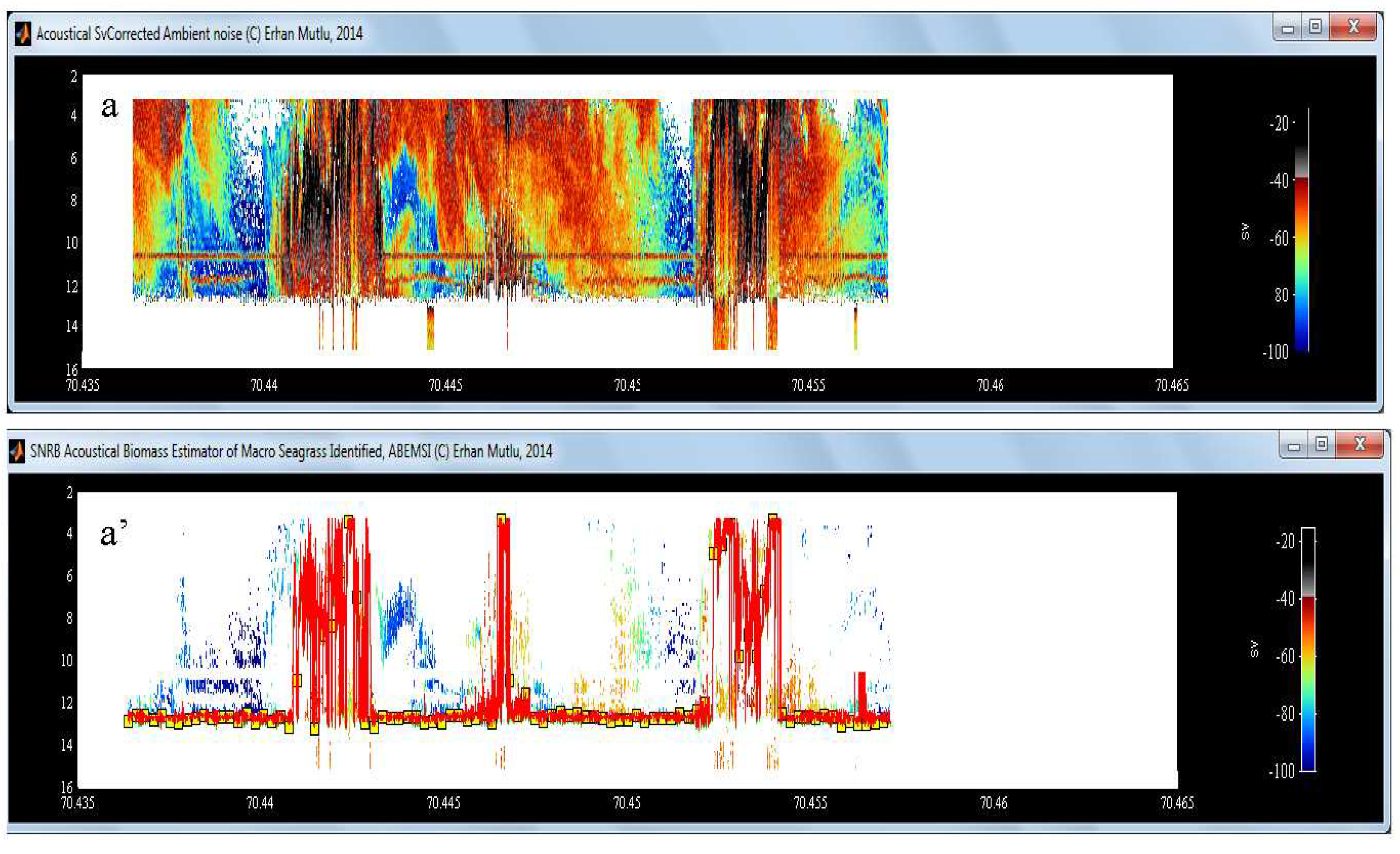
The SNR estimates were based on three different algorithms in the present study modifying the procedure slightly in a script, AbemsiR1 (see Mutlu and Balaban [58] for description of the abbreviation). Two different measurements were pre-required for the present study. These measurements would be fundamental reference data in a priority to the SNR solution. The background natural noise including electrical and physical ambient noises changes in time and space. Therefore, at least one measurement is recommended for each of two noise types during an acoustical survey. During the survey with a research vessel, some other acoustical devices are used for the measurements of other purposes such as water current, bottom depth sounding, fishing net sounding etc. Such instruments can interferer the echoes of the study echosounder, and are classified as artificial noise-generators. Furthermore, the interferences occurred owing to biological sound sources and sheering of echo returned from the bottom with echo (pulse) of the next pinging. Both noise measurements can be performed using listening mode of the echosounder and used as a hydrophone. During the present study, one noise measurement was conducted switching off the depth reader, fish finder (echosounder) or similar acoustical devices (e.g., ADCP) of the research vessel (ship) (Figure 2a) and the next measurement switching on the devices (Figure 2b).
Three methods for removal of background noise (b), interference (i) and variety (surface, volume and bottom) of reverberations (r) were cased conditionally with some additive functioning ranges (see Table 2, Figure 9) between measured (MSNR) [79] and expected (ESNR) data (e.g., in Figure 2) as follows:
if MSNRb > ESNRb, removal of the data,
if not, set ESNRb into the acoustical data for the corresponding depth, instead of -999 as suggested by De Robertis and Higginbottom [79],
if MSNRir > ESNRir, removal of the data,
if not, nothing done,
if MSNRir/MSNRb > a criterion value automatically estimated between the ratios for each acoustical data file, removal of the data,
if not, nothing changed (this option is useful tool for detection of air-bubble generated by SCUBA divers).
The expected SNR (ESNR) versus the water column depth was estimated using a logarithmic regression between acoustical data (Sv) without Time-Varied-Gain (TVG, one-way transmission loss, TL=20logR + 2Rα, where R is the range in m, and α is absorption coefficient in dB/m) and depth for both background noise (Figure 3a) and interference (Figure 3b).
2.3. Algorithm of “SheathFinder” & Leaf length and biomass (Sheathfinder1, and 2)
This script consisted of sections of simultaneous removal of weak and strong scatterers, and simultaneous calibration and fixation of the leaf and sheaths or vertical rhizome of Posidonia oceanica (Figure 4). All processes were visually performed looking at the calibration file. Visual calibration file is pre-required before switching to the next real process to estimate the biometrics. The calibration file possesses a section having the meadow (Figure 4d,e). In some temporal cases, the vertical rhizome and sheath could be too short for the detection or within the deadzone [5]. In these months, the filtration continues until leaf parts near the sheaths disappear on the enhanced echogram.
After fixation of the sheaths, the algorithm seeks the count-to-count echo upward to determine the leaves until there are a few gaps between the successive counts. The rule for the determination is that volume backscattering strength has to be in a decreasing trend from the bottom to top of the leaves.
After completing the seeking above the dead zone, this height reads the leaf length in a precision of one-eighth of the pulse width depending on number of strata entered in “Visual Analyzer”. Thereafter strong scatterers suchlike fish are removed from each leaf, and the EDSUs (Sv: volume backscattering strength in dB/m3 and Sa: area backscattering strength in dB/m2) are calculated following the methods as suggested by Simmonds and MacLennan [52]. Besides, the algorithm discards echo without sheath, and categorizes that as a false leaf (Figure 4e).
After finishing processing the acoustical data of a file, leaf biomass is assessed using different EDSUs in relations to the biometrics of the meadow in time [60]. Of the six different temporal relationships [60], the algorithm choices right month matched with month of the acoustical data over yearday. It shall choice the closest month if the yearday of the data is outside the six months.
Methodologically, each script needs an input file or data produced as an output file in MatLab format (*.mat) by the previous script throughout AbdezdeR1 to Sheathfinder2. Initially, AbdezdeR1 only needs output files in CSV format, processed by “Visual Analyzer” since the package of POSIBIOM cannot directly read file.dt4 in the current status.
The package is installed according to window size based on the pixels of the monitor or display owned by the users.
3. Results
Besides the data (acoustical data in *.CSV to *.mat) and auxiliary (baseline or coast map in format of *.bln to *.mat, reference noises in *.CSV, sheath calibration in *.mat, and coast blanking in *.bln to *.mat) files opening/loading, a main menu for controlling all processes is configured in a window called POSIBIOM (Figure 5).
3.1. Flowchart of POSIBIOM
The diagram shows the flowchart in order to finalize all analyses (Figure 5). There is also an option called “Tools” to plot results for leaf length and biomass distribution in format contour or line on the map.
To load the data for acoustical or other type data, opening in “File” is associated with that of Microsoft Window, embedded in the MatLab. For each analysis, opening files is specifically called from the menu (Figure 5). Files for analysis of “Lost Bottom” are opened in format of “*. CSV”, output of Visual Analyzer. The next analyses use format of “*.mat” as output of the previous successive analysis.
The output files are saved in a folder “AbdezdeOut”, created by the package, under the folder where the user opens the data for “Lost Bottom” analysis. The next analyses save the outputs into a folder “AbemsiOut”, and “PosiBiom” for “Noise & Reverberation”, and “SheathFinder & Leaf and Biomass” algorithms, respectively in the way aforementioned. In other word, the previous output files become input files for the next analysis. Output file of the last analysis (Figure 5) is in format of “*.xls*” for the users to use the data for their different purposes.
3.2. Lost Bottom and Dead Zone
This algorithm is purposed to correct the lost bottom, and then to estimate dead zone depth using three different equations (Equations, 1-4). After opening single or multiple input data files the users want to process (Figure 5), the algorithm needs also to open a coastline file from ‘Base Line for Map” before starting the analysis clicking “Lost Bottom” in “Analyses” in POSIBIOM menu (Figure 6).
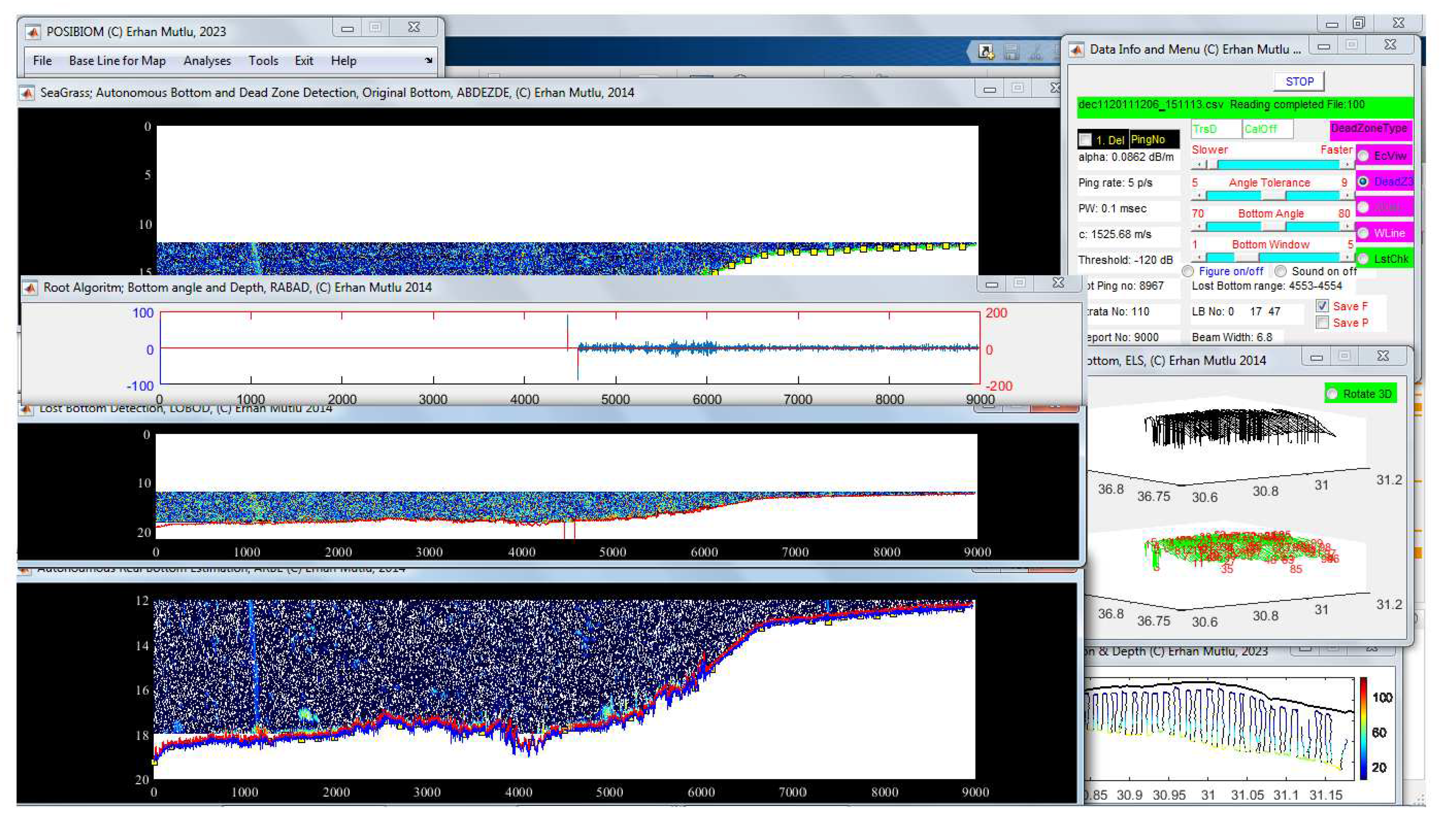
The algorithm starts to read each of the files sorted in an alphabetic order of A-to-Z after starting the analysis (Figure 7), and then a window appears to control the analysis (Appendix 3) and get information of the acoustical data and echosounder configuration during the sampling (Figure 7, Appendix 4). After all setting (transducer depth, calibration offset, types of dead zone estimates, save etc., Table 1) is performed in the window, the analysis proceeds tapping button START (Figure 7). Description of each option in Figure 7 is presented in Table 1 with their functions, case to use, recommendation and possible negatives.
Figure 7.
Graphical menu for control, configuration and info menu of “Lost Bottom” (see Table 1 for actions of each coded option and function with number).
Figure 7.
Graphical menu for control, configuration and info menu of “Lost Bottom” (see Table 1 for actions of each coded option and function with number).
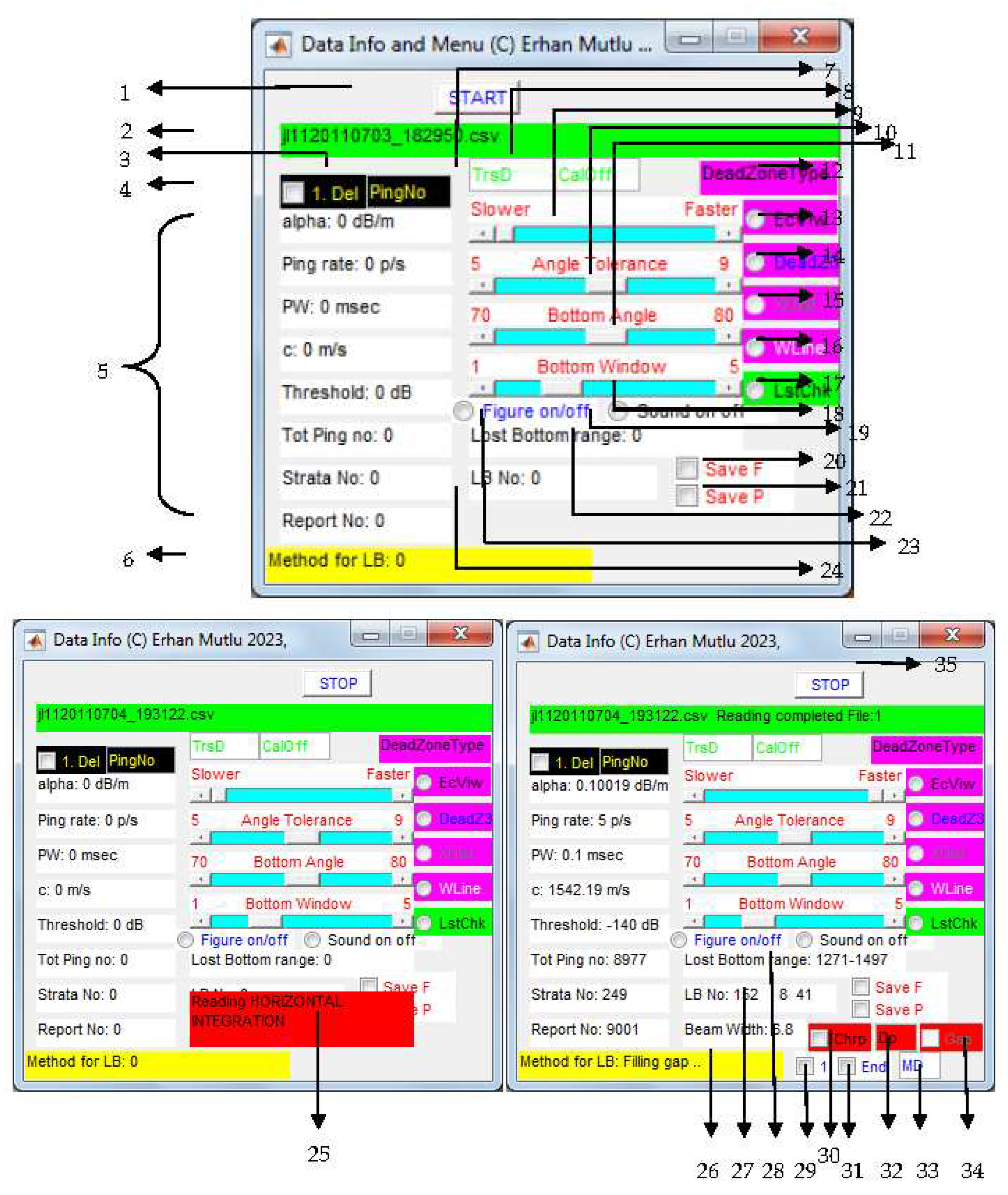
During the process with the “Lost Bottom”, enhanced echogram first appears in pings versus depth for unprocessed acoustical data with marks of the estimated lost bottoms in green lineation (Figure 8a). These lineation occurred based on the algorithm of bottom angle and bottom depth in the adjacent real bottoms (Figure 8b, the figure appearance is optional because of some cases, no 23 in Table 1). As the analysis progresses, bottom depth correction starts from the beginning to the end of the pings (Figure 8c, the figure appearance is optional because of some cases, no 23 in Table 1). If there is any spurious scatterer through the water column in front of the bottom, the processing cleans them in order to reach the bottom. Nevertheless, original acoustical data are saved into output file. After finishing the analysis for the lost bottom, the algorithm estimates the dead zone depths using the equations user selects, and then final enhanced echogram comes out in the screen. If user checks option “save P”, the final echogram is saved as format of *.jpeg (*, input filename). If user checks option “save F”, the final results with the variables necessary to the next analysis is saved as *.mat (*, input filename) to folder “AbdezdeOut”. Finally, the corrected bottom depth is plotted in line on a map after correction rate info appears on a 3D-plot to be checked by user to see uncorrected and corrected bottom depths (Figure 8e, e’, respectively).
From this example in Figure 8, the result showed a significant of correction rate on comparison of plot in Figure 8e with that in Figure 8e’. Overall, goodness of the correction was estimated in a percentage of more than 95 after all files (approximately 4000 files belonging to different seasons and years) were analyzed by the “Lost Bottom”. The plots in Figure 8d, e are reset every 100 files processed, and the analysis then needs to press START to continue the next files.
3.3. Noise, Reverberation and Interference
This algorithm is purposed to remove background natural noise, reverberation and interference (artificial noises) using three different conditional functions based on the SNR (Figure 9). After opening single or multiple input data files the users want to process (Figure 5), the algorithm also needs to open a coast file from ‘Base Line for Map” in the main menu, and needs two different noise files as described in Figure 2, Figure 3 and Figure 5 before the analysis. Starting the analysis is performed clicking “Noise” in the “Analyses” in the POSIBIOM menu (Figure 6). This algorithm first runs a subcall in association with “Noiseback1” to estimate the expected SNR (ESNR) for background noises and interferences (Figure 3).
The algorithm “Noise & Reverberation” is achieved depending on the configuration the users perform to configure the options flexibly; particularly for the reverberation intensified at the surface and water column (volume reverberation) (Figure 10a). The surface reverberation is sourced by the wavy sea, strong winds rocking/rolling the ship, and speed of its propel at stop.
The interference had different patterns in relation to the bottom depth, and pulse width, ping rate and frequency of the ship and researcher echosounder (Appendix 5).
The menu needs to enter an approximate maximum canopy height of the seagrass and the transducer draft depth installed during the survey, and if no entry, the default values appear (Figure 9, Table 2).
Figure 9.
Graphical menu for control, configuration and info menu of “Noise & Reverberation” (see Table 2 for actions of each coded option and function with number).
Figure 9.
Graphical menu for control, configuration and info menu of “Noise & Reverberation” (see Table 2 for actions of each coded option and function with number).
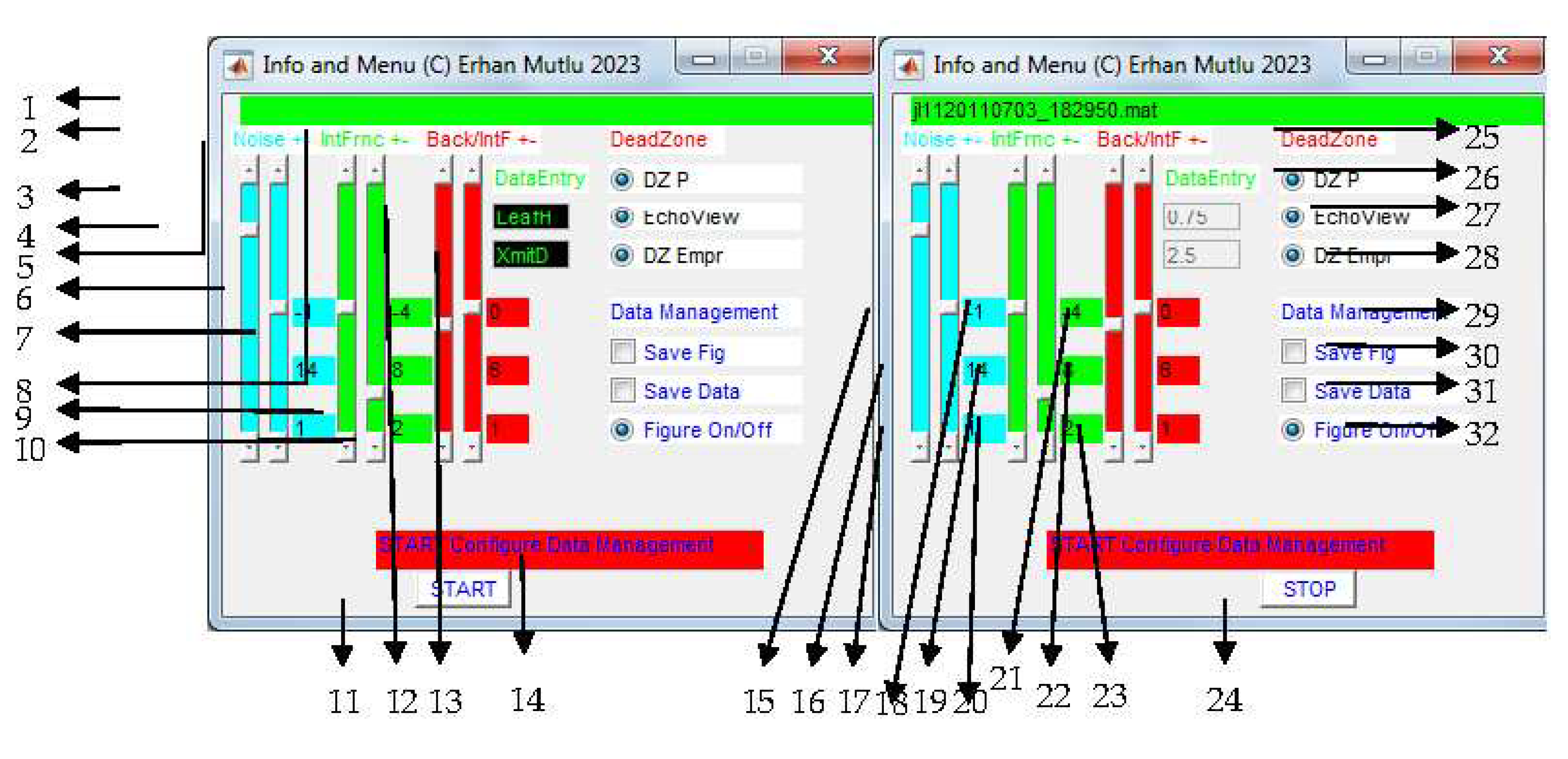
After finishing to run “Noiseback1”, the program calls a subprogram“Sheatfinder2” to start the process for the removal of the spurious echoes such as the noises, and reverberations. The subprogram demonstrates first output data, processed by the “Lost Bottom”, in an enhanced echogram (Figure 10a), and bottom depth and average dead zone line estimated by the methods the user checks in (option numbers of 26-28 in Figure 9). If any method is not checked by the user during the processing by “Lost Bottom”, the method option is disabled automatically in the analysis of “Noise & Reverberation” (Figure 9). The algorithm starts to fix the noises and reverberations for the removal after the trail of three conditions (Figure 10b, c) between the measured and expected SNR. Thereafter, the output file with the variables (Figure 10d) necessary to the next analyis, “SheathFinder, Leaf & Biomass” will be saved as format of “*.mat” in to a folder, “AbemsiOut” under folder, “AbdezdeOut” if the user wants to save the outputs (Figure 9, function no 31).
Figure 10.
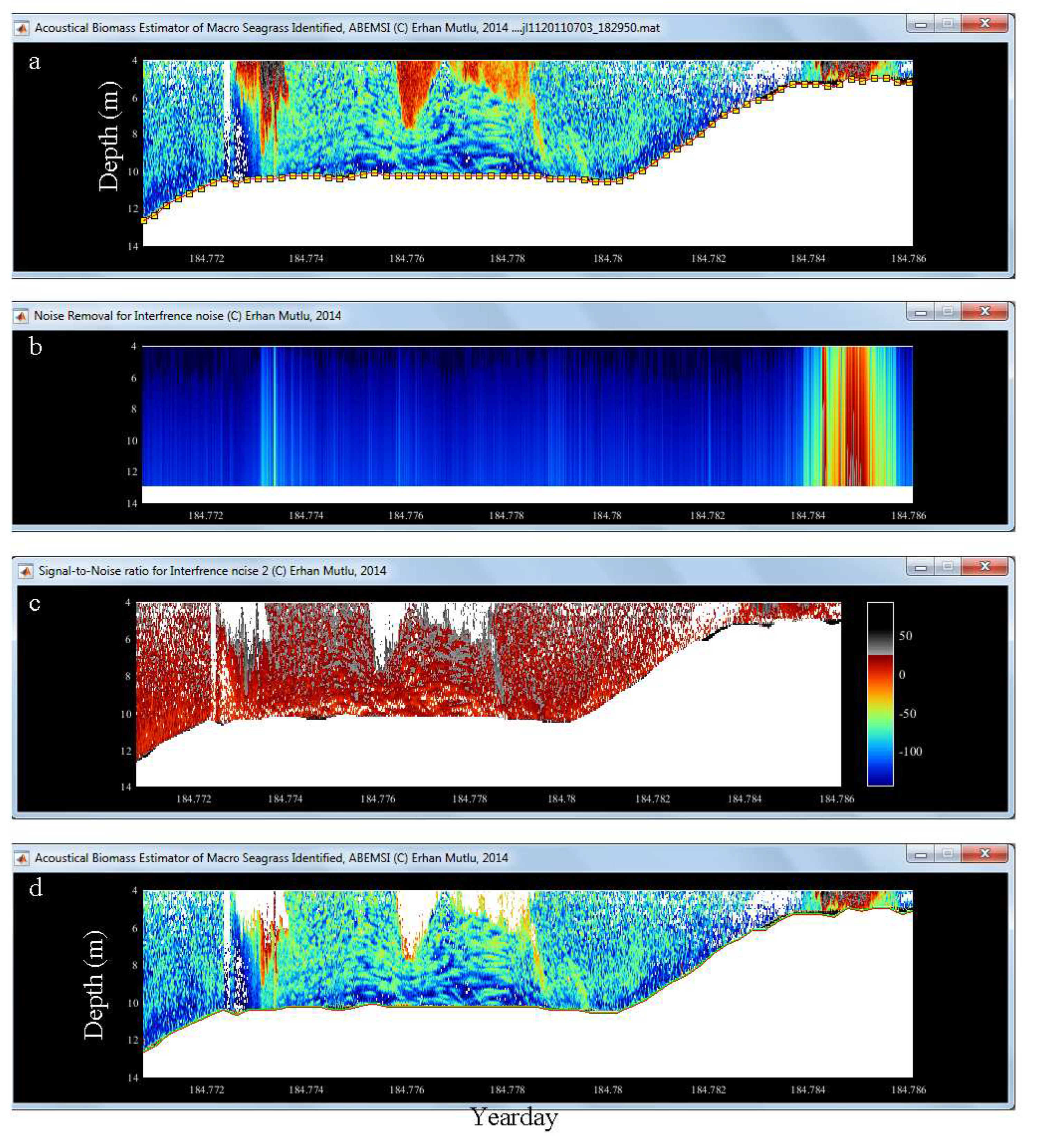
Graphical outputs of the “Noise & Reverberation” analysis. a) Enhanced echogram before the start of the analysis, b) an algorithm to figure out detection of the overall noises, spurious echoes (optional), c) the SNR for each background natural and artificial noise (optional), d) removed noises and reverberations, in this example the configuration needs optimum adjustments furthermore to remove the entire reverberations.
Figure 10.
Graphical outputs of the “Noise & Reverberation” analysis. a) Enhanced echogram before the start of the analysis, b) an algorithm to figure out detection of the overall noises, spurious echoes (optional), c) the SNR for each background natural and artificial noise (optional), d) removed noises and reverberations, in this example the configuration needs optimum adjustments furthermore to remove the entire reverberations.
The noise, especially interferences had different patterns extending down to the bottom in time and space (Appendix 5). This situation creates a lot of negative and spurious sources suchlike fake acoustical characteristic similar that of the sheaths and vertical rhizome. Besides, there is different reverberation rather than that generated by the ship propel; for instance, that generated by SCUBA divers as studying a purpose within beam of the transducer (Appendix 6). During the analysis both unrecovered and unfixed noises and reverberations are removed by the next analysis, “SheathFinder, leaf & Biomass”, and echoes through the canopy height are kept to the next analysis.
3.4. Leaf and Biomass Estimation
Recognition of different traits of P. oceanica in the algorithm was performed basing the descriptions on the experimental results obtained from Mutlu and Olguner [60]. After cleaning out of the spurious echoes from the acoustical data, the algorithm gives an opportunity for visual calibration to fix the seagrass (Figure 4). Therefore, this algorithm gives a favor for the users which are not much familiar with the acoustical theory. For the calibration, three sliders which guide the users with each of color scale specific to the each slider are available to remove weak, strong scatterers, and to fix the leaf and sheath or vertical rhizome, respectively (Table 3, Figs. 4, 11). For that, user needs only to load a file containing the seagrass from the main menu, POSIBIOM (Figure 5). Before starting the analysis, both acoustical and calibration data files are required to open (Figure 5). At the same time, the coast file is needed to plot results on map.
Compared to the other algorithms (Figure 7 and Figure 9), the present algorithm is the easiest and simplest graphical demonstration during the usage (Figure 11). There are some options to save or plot the estimated results (leaf biomass and length) based on the different EDSUs. Overall, the biomass estimate based on Sv is plotted on a map on the colored trackline (Appendix 7c, d). For the contour or line plots, a further option called ‘Tools’ was embedded in the main menu with some more graphical properties.
During the analysis, the biomass is estimated using a combination of Sv and Sa with eight equations formulated by Mutlu and Olguner [60]. When tapping “Result Table”, the results flow down ping-to-ping, but this option slows down the analysis. The algorithm saves the results comprising of three different estimate of the biomass, including other informative variables (file name, geographical coordinate, yearday informing time in format of day,hrs+min+s of a day, bottom depth, dead zone depth, canopy height (leaf height), the biomasses (based on Sv, Sa in “Cut” experiment, Sa in “Leaf” experiment [60], and month range of which the equation is used to estimate biometrics (Figure 12).
During the analysis, the algorithm starts to scan structure suchlike the sheath or vertical rhizome of the seagrass in ping-to-ping depending on the vertical resolution analyzed with “Visual Analyzer” (Figure 12a). The green scanning vertical line proceeds slower when determining the sheaths than that during absence of sheaths in the ping. There are two theories applied to remove the fake seagrass; one is presence/absence of the sheaths, and another is structure suchlike the sheaths whether to have real leaf or not as described in Material and Methods.
After completing to scan the sheaths and leaves, strong scatterers like fish individuals among the leaves are removed according range of the expected threshold of the Posidonia [60]. The next step is the biomass estimates of the leaves which are regressed with seasonal equations according the current sampling month [60], followed by saving the output data in a format of “*.xls” without variable names into an automatically created folder “PosiBiom” The variable names are in the order of each column as follows; geographical coordinates (latitude, longitude), yearday, bottom depth, canopy tip depth, leaf height (canopy height since orientation of leaves standing on the bottom; right, semi-flat and flat position, [62]), and three different successive biomasses (g/m2) estimated by Sv and Sa (“cut experiment”), and leaf calibration (“leaf experiment”) [60]. There is an auxiliary script, namely ”PosiDrwTool” in “Tools” of the main menu, POSIBIOM to draw distribution of the estimates in a format of trackline or contour (Appendix 7 and Appendix 8).
4. Discussion
The present study has discussed the advantages and disadvantages of the algorithm, POSIBIOM with the other acoustical commercial software to estimate bottom type and vegetation since the POSIBIOM is a production of the first study for Posidonia oceanica and its biometrics. Some scripts of the algorithm were related to solution of the general acoustical problems (e.g., lost bottom correction and noise and reverberation removal) during the post-processing of the acoustical data purposed for the other studies, such as fisheries acoustics. For such problems, there are commercial and professional software. In their some cases, a manual intervention is needed to correct the bottoms even if they have many functions for this matter. The mapping of macrophytes can be accomplished with the software developed for the submerged vegetation (Echo Submerged Aquatic Vegetation; EcoSAV, Visual Habitat and Visual Aquatic) by BioSonics Company. Further methods of vegetation acoustics were developed based on algorithms to classify bottom types [63,64,65,66]. They are OTCView, Echoplus, BioSonics VBT (Visual Bottom Typer), and EchoView [67,68,69,70]. However, previous studies on the vegetation acoustics have remained at the assessment of percent coverage and canopy height of the seagrass (e.g., van Rein et al. [50]; Lee and Lin [80]) depending on the limitation of echosounder parameters [81]. Unlike the POSIBIOM, there is overall a maximum bottom depth restriction with a depth value entered in the software to remove suchlike the seagrass or macrophytes at the greater depth. There were two attempts to calibrate the acoustical data to estimate the biometrics of the seagrass by developing the nonprofessional algorithm; one was based on data of VBT process [59], and the next one was based on “SheathFinder” to fix the sheaths/vertical rhizome [58]. The present study modified and revised the nonprofessional algorithms completely and significantly to be used professionally for the seagrass studies.
Regarding to the package POSIBIOM, one issue is the avoidance from the usage of the destructive methods to study the meadows under the protection [34,35,36]. Besides, the previous remote sensing techniques produced only coverage and mapping of the different habitats (e.g., Fakiris et al. [48]; Dimas et al. [49]). Compared to the techniques, the acoustical method is faster, more precise, and easier to ground-truth the data [2,50], and develop the algorithms to remove spurious scatterers [51]. Another issue is detection of the seagrass by the acoustical frequency. The meadow is detected well by a frequency of 206 (200) kHz to assess biomass variables even if the higher frequency (420 kHz, Biosonics inc.) is recommended to study the seagrass and vegetation acoustics. Quintino et al. [82] recommended 50 kHz to study soft bottom classification, but 200 kHz is good effective for the classification of the bottom types including seagrass.
Vegetation acoustics is not however easier at practice to process its data than the fish acoustics. The fisheries acoustics had many problems overcome during the processing [52]. In many cases, the macrophytes and seagrass had unstable relationships specifically with oscillation between the EDSUs and biometrics in time and space [60,61]. These all relationships biased the estimates besides the other scatterers were available suchlike as epiphytes on the leaves and fishes among the seagrass [35,59,61]. The meadow showed inconsistent linear relationships in some seasons [60] when its biological and physiological activities were intensified [83]. Another seagrass, C. nodosa produced a more stable relationships in time than P. oceanica performed [60,61]. The POSIBIOM regarded these matters to estimate biomass by using three different equations of the relationships established in each season [60]. However, any flower (only one flower found) and fruit of the meadow was not encountered during the all surveys of the present study. The flower and fruit which occurred often in the West Mediterranean Sea [84,85] would change the acoustical traits of the meadow in other parts of the Mediterranean coasts. The main factor producing the variation in the estimates is the strength and magnification of the physiological activities of the meadow, calcification, oxygen gas releasing, beam pattern (orientation), age/type (juvenile, middle and adult leaves) and hardness of the leaves, and bottom depth of the occurrence of the meadow [60,61,62,86,87,88,89,90]. The relationships used in the present study were established by means of an in/ex situ study at a bottom depth of 15 for each season. The 15 m was a critical range with its inconsistent biometrics in high variation between shallow and deep Posidonia [5,18]. The fish removal was standardized according to the results of the acoustical ranges of the meadows, but possible significant epiphytes could be disregarded for the removal. For this, SCUBA sampling was needed for assess acoustical contribution to the EDSUs of the meadow leaves by solving the forward model solution [60]. This was not a practical way for the clear biomass estimates with frequent SCUBA samplings as a destructive method. Mutlu and Olguner [61] estimated the contribution of a calcareous alga, Pneophyllum fragile to the EDSUs of leaves of C. nodosa, and the contributions remained below the threshold of the leaves depending on abundance (ind/m2) of the alga. Another calcareous alga, Hydrolithon boreale occurred recently on leaves of P. oceanica at the present study, its abundances were found to be low as compared of that of C. nodosa [35,61].
The POSIBIOM could be the best offer currently for the biometric estimates regarding the matters aforementioned, and some improvements are needed during the next studies to decrease possible disadvantages. There are some biases in estimating the biomass and bottom coverage compared to the estimates by SCUBA (Appendix 8 and Appendix 9). This could be due to misestimates of bottom recovery for the coverage and the equations established at 15 m for the biomass [60]. A bottom depth of 15 m was found to be critical depth for occurrence of the high variations of the biometrics [5,18]. The negatives/troubleshooting were discussed for each algorithm in Table 1, Table 2 and Table 3.
As a conclusion from the present to future studies featured to improve the algorithms;
The algorithm would open acoustical data of the different echosounders manufactured by other companies rather than that by BioSonics,
A way would be developed for reading the acoustical row data directly, needless of the post-processors,
The debugs would be considered to get rid of them if the feedback about that was returned by the users after the package would be a profession version converted to a programming language of C,
The multi-frequencies would be applied if the data was collected, and then the algorithm would be figured out and configured accordingly,
The experiments would be repeated to establish the relationships between the EDSUs and biometrics at the different bottom depths, else than 15 m,
Leaf types would be also taken into account of the equations of the relationships,
Mapping the results would be associated with different types of the coastal map,
Eventually, the software of the package would be hardware connected to the echosounder, which needs too much works associated with the electronics.
Author Contributions
Conceptualization, E.M.; data collection, E.M.; methodology, E.M.; writing-original draft preparation, E.M.; validation, E.M.; formal analysis, E.M.; investigation, E.M.; supervision, E.M.; funding acquisition, E.M. Author has read and agreed to the published version of the manuscript.
Funding
This research was funded by TÜBİTAK (The Scientific Technology and Research Council of Turkey), grant no: 110Y232, 117Y133.
Institutional Review Board Statement
Not applicable.
Informed Consent Statement
Not applicable.
Data Availability Statement
Not applicable.
Acknowledgments
The present study was carried out within the frameworks of two projects (grant no: 110Y232, 117Y133) funded by TÜBİTAK (The Scientific Technology and Research Council of Turkey). I thanked researchers and scholars of the projects and crew of the R/V “Akdeniz Su” for their helps on board and at laboratory.
Conflicts of Interest
The author declare no conflict of interest.
Appendix A
Appendix 1.
Coast line file downloaded from Marine Region [76] and then converted to formats of SURFER (Golden Software) and MatLab (MathWorks inc.). Each colored area is a large sector in polygon (13 polygons) consisting of polygons of the islands to use for mapping and blanking data outside the Islands as formatted by Marine Region [76].
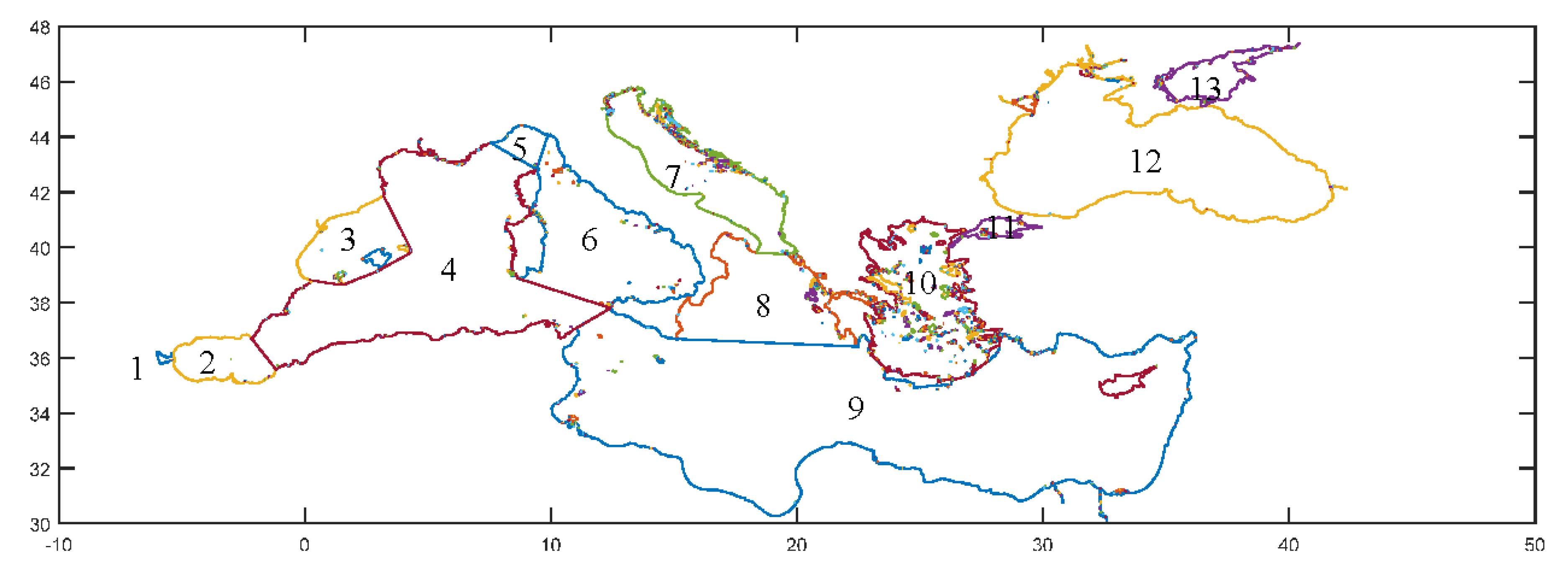
- Gibraltar Straits
- Alboran Sea
- Balearic Sea
- West Mediterranean Sea
- Ligurian Sea
- Tyrrhenian Sea
- Adriatic Sea
- Ionian Sea
- East Mediterranean Sea
- Aegean Sea
- Sea of Marmara
- Black Sea
- Azov Sea
Appendix 2.
Automatic appearance of option in a case of existence of misestimated bottom at the first pings owing to the volume or surface reverberations or the interferences.
Appendix 2.
Automatic appearance of option in a case of existence of misestimated bottom at the first pings owing to the volume or surface reverberations or the interferences.
Appendix 3.
Screen shot of analysis “Lost Bottom” during the processing. Two figures in the middle of left panel appear optionally when function “Figure on/off” is on.
Appendix 3.
Screen shot of analysis “Lost Bottom” during the processing. Two figures in the middle of left panel appear optionally when function “Figure on/off” is on.

Appendix 4.
Echosounder parameters during the data collection and *configuration parameters of Visual Analyzer during the post processing (see Figure 7).
Appendix 4.
Echosounder parameters during the data collection and *configuration parameters of Visual Analyzer during the post processing (see Figure 7).
| Info variables | Description |
|---|---|
| alpha | Absorption coefficient |
| Ping rate | Pulse rate per second |
| PW | Pulse width |
| c | Sound speed |
| Threshold | Minimum data collection threshold |
| Tot ping no* | Total number of pings |
| Strata* | Number of stratum (vertical resolution) |
| Report No* | Number of reporting data (horizontal resolution) |
| Beam width | Angle of main lobe of beam |
Appendix 5.
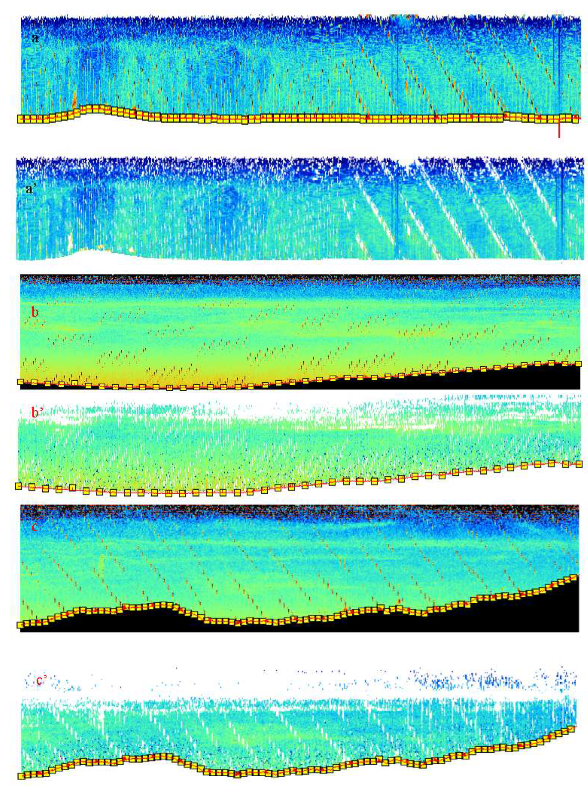
Removal of background noises; different patterns of the interferences. a, b, c) original data, and a’, b’, c’) removal of the interferences, respectively.
Appendix 5.
Removal of background noises; different patterns of the interferences. a, b, c) original data, and a’, b’, c’) removal of the interferences, respectively.
Appendix 6.
Removal background noise and reverberation; different patterns of the surface and volume reverberations produced by SCUBA divers, a) original data, a’) removal of the reverberations, respectively.
Appendix 6.
Removal background noise and reverberation; different patterns of the surface and volume reverberations produced by SCUBA divers, a) original data, a’) removal of the reverberations, respectively.
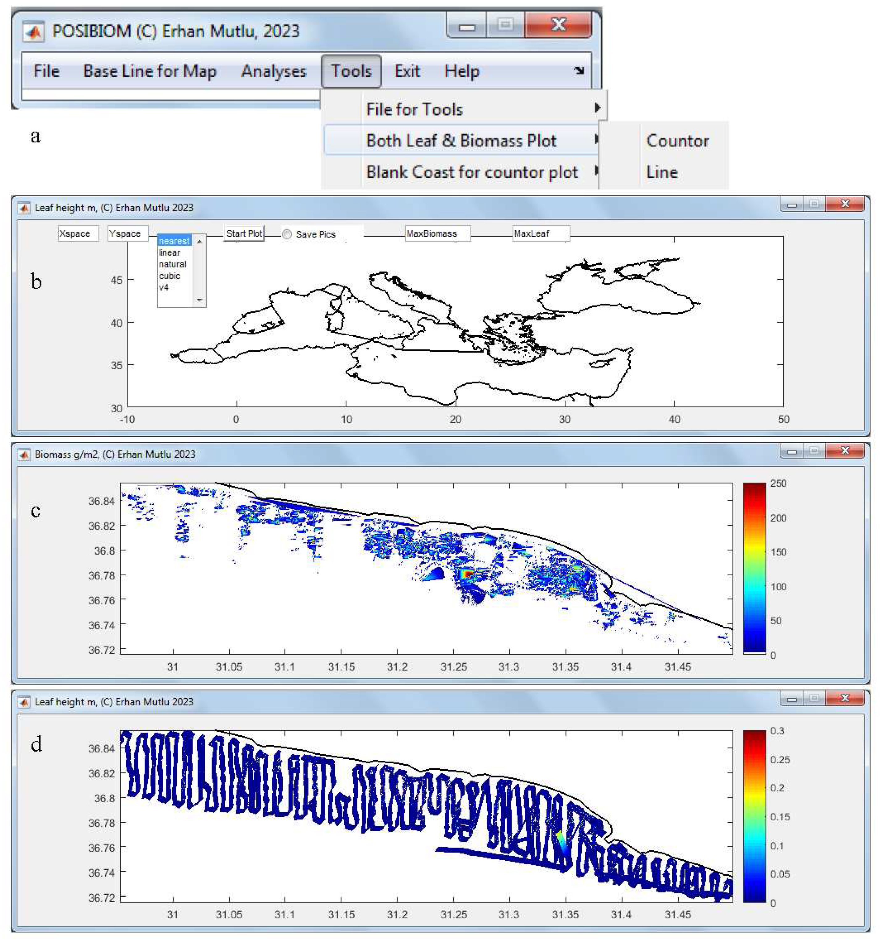
Appendix 7.
Tools menu to load files (a), to configure the plot of the map for instance here biomass (g/m2) in contour (b, c) or leaf length (m) in trackline (d) depending on maximum value the user sets. When selecting contour plot, some entries appear to configure interpolation to make grid (Xspace; longitude versus Yspace; latitude), interpolation type and save of the figure (b, c) and when selecting the line plot (b, d), an entry only for line width. The data was an example from July 2011 (c, d).
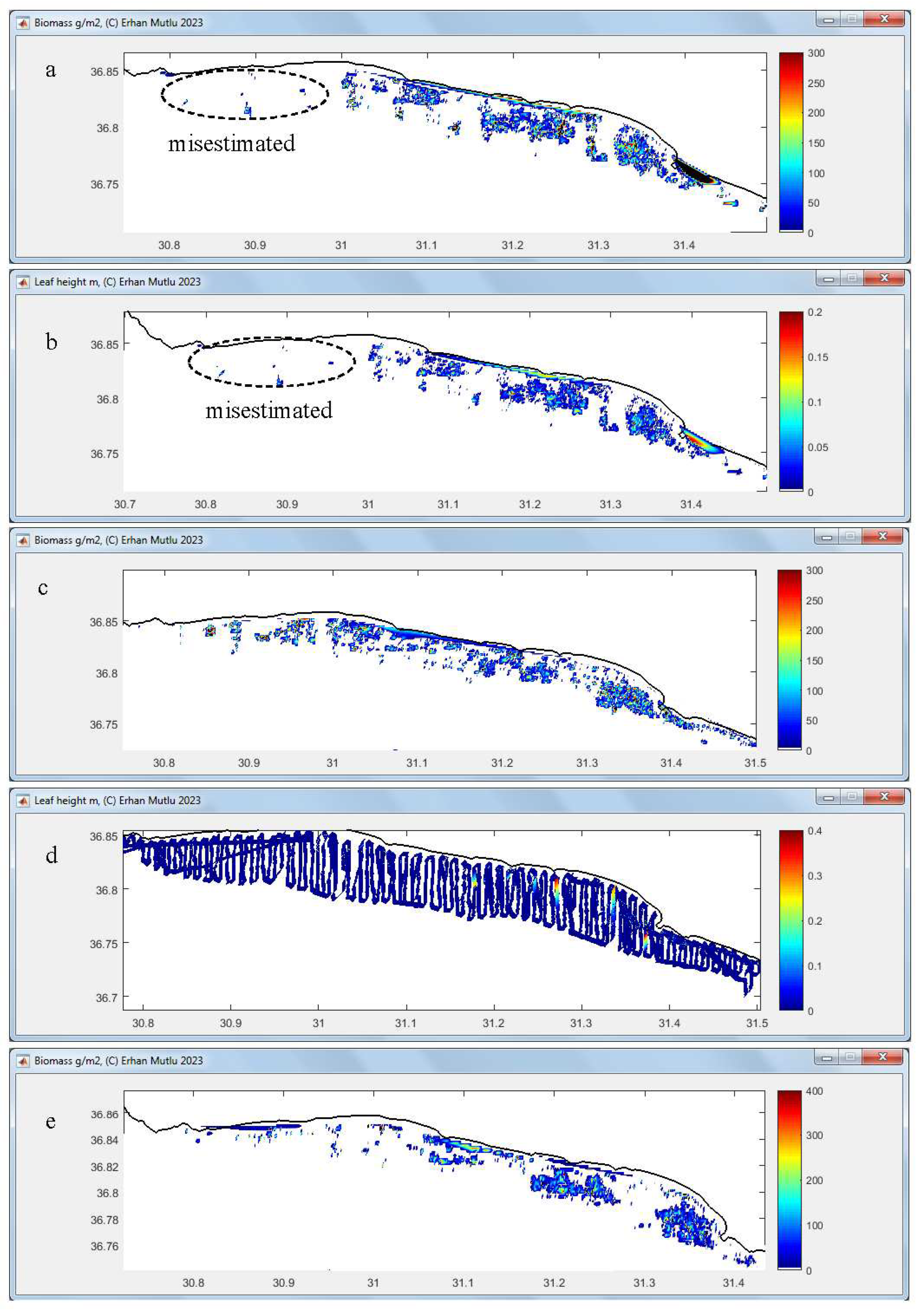
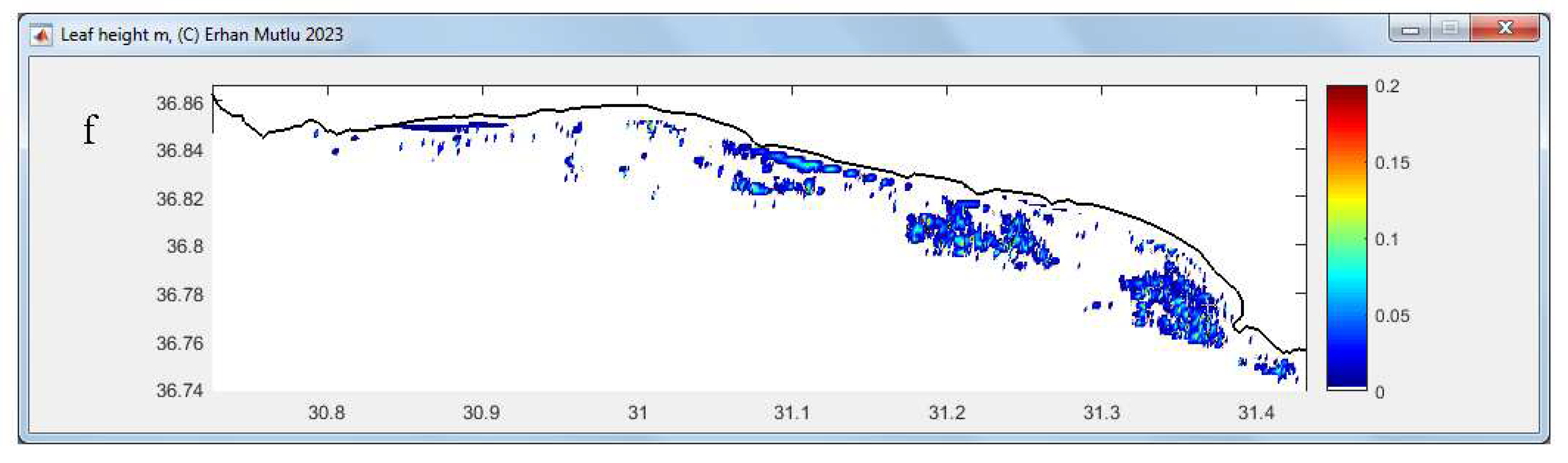
Appendix 8.
Outputs of ‘Tools” of the package program: a) leaf biomass ditribution (g/m2), and b) leaf length (m) in contour mode in December 2011, and c) and d) in contour mode and line mode in January 2012, and e) and f) in April 2012, respectively.
Appendix 8.
Outputs of ‘Tools” of the package program: a) leaf biomass ditribution (g/m2), and b) leaf length (m) in contour mode in December 2011, and c) and d) in contour mode and line mode in January 2012, and e) and f) in April 2012, respectively.
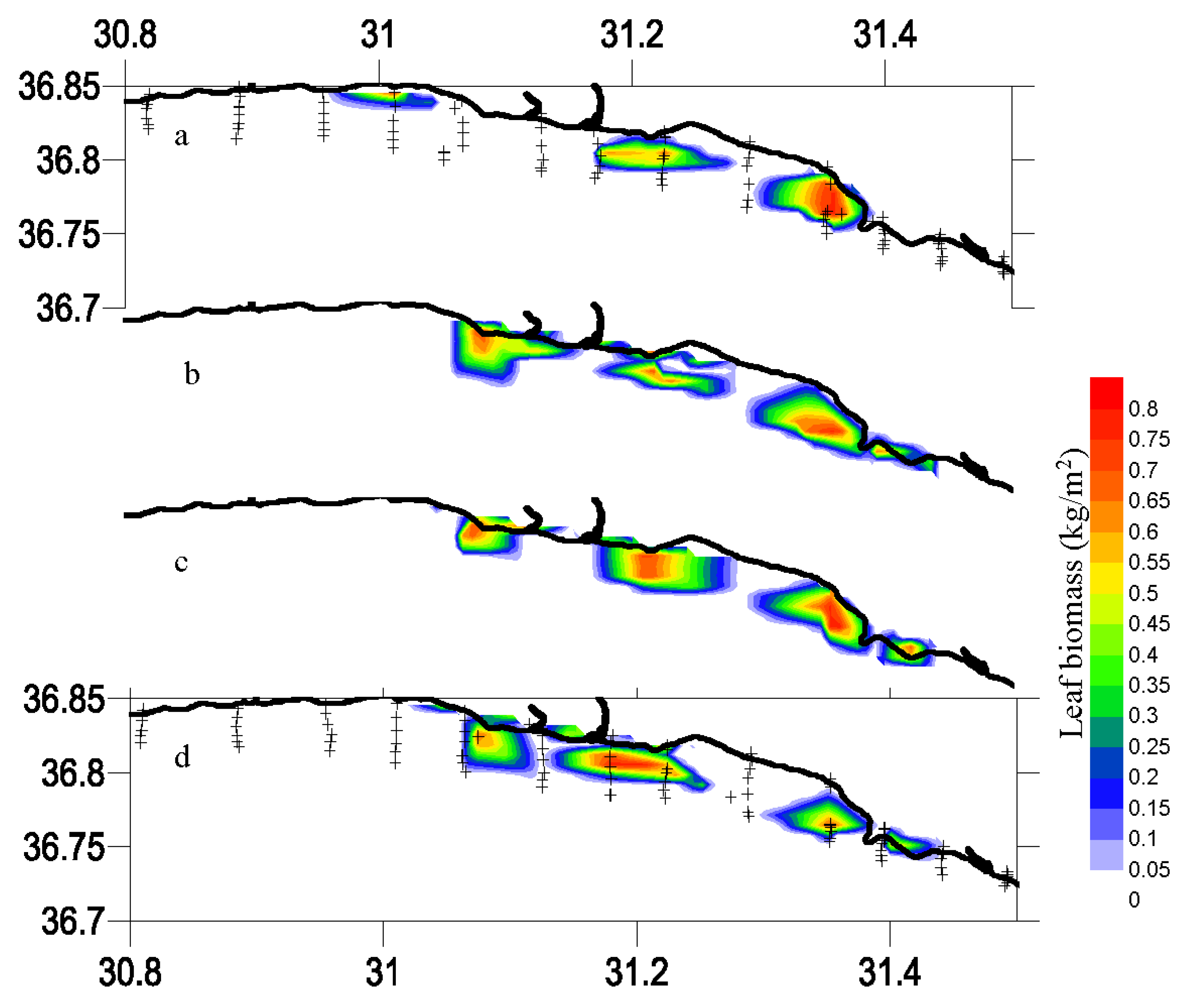
Appendix 9.
Posidonia oceanica: leaf biomass (kg/m2) estimated from SCUBA sampling in December 2011 (a), January 2012 (b), April 2012 (c), and July 2011 (d) to compare with estimated with acoustics (see Appendix 7 and Appendix 8 for the comparison). (+: sampling stations by SCUBA).
Appendix 9.
Posidonia oceanica: leaf biomass (kg/m2) estimated from SCUBA sampling in December 2011 (a), January 2012 (b), April 2012 (c), and July 2011 (d) to compare with estimated with acoustics (see Appendix 7 and Appendix 8 for the comparison). (+: sampling stations by SCUBA).
References
- Colantoni, P.; Gallignani, P.; Fresi, E.; Cinelli, F. Patterns of Posidonia oceanica (L.) DELILE Beds around the Island of Ischia (Gulf of Naples) and in adjacent waters. PSZNI Mar. Ecol. 1982; 3(1), 53–74. [Google Scholar] [CrossRef]
- Brown, C.J.; Smith, S.J.; Lawton, P.; Anderson, J.T. Benthic habitat mapping: A review of progress towards improved understanding of the spatial ecology of the seafloor using acoustic techniques. Estuar. Coast. Shelf Sci. 2011, 92, 502–520. [Google Scholar] [CrossRef]
- Pal, D.; Hogland, W. An overview and assessment of the existing technological options for management and resource recovery from beach wrack and dredged sediments: An environmental and economic perspective. J. Environ. Manag. 2022, 302, 113971. [Google Scholar] [CrossRef] [PubMed]
- Boudouresque, C.F.; Meinesz, A. Découverte de l’herbier de Posidonies. Cahier Parc Nation Port-Cros. 1982, 4, 1–79. [Google Scholar]
- Mutlu, E.; Olguner, C.; Gökoğlu, M.; Özvarol, Y. Seasonal growth dynamics of Posidonia oceanica in a pristine Mediterranean gulf. Ocean. Sci. J. 2022, 57, 381–397. [Google Scholar] [CrossRef]
- Vacchi, M.; De Falco, G.; Simeone, S.; Montefalcone, M.; Morri, C.; Ferrar, M.; Bianchi, C.N. Biogeomorphology of the Mediterranean Posidonia oceanica seagrass meadows. Earth Surf. Proc. Land. 2017, 42, 42–54. [Google Scholar] [CrossRef]
- Spalding, M.; Taylor, M.; Ravilious, C.; Short, F.; Green, E. The distribution and status of seagrasses. In: Green, E.P.; Short, F. (Eds.), World Atlas of Seagrasses. University California Press, 2003, pp. 5–26.
- Aires, T.; Marbà, N.; Cunha, R.L.; Kendrick. G.A.; Walker, D.I.; Serrão, E.A.; Duarte, C.M.; Arnaud-Haond, S. Evolutionary history of the seagrass genus Posidonia. Mar. Ecol. Prog. Ser. 2011, 421, 117–130. [Google Scholar] [CrossRef]
- Bianchi, C.N.; Morri, C.; Chiantore, M.; Montefalcone, M.; Parravicini, V.; Rovere, A. Mediterranean Sea biodiversity between the legacy from the past and a future of change. In: Science N (ed) Life in the Mediterranean Sea: a look at habitat changes, Stambler, N.; Publishers, New York, 2012, pp 1–55.
- Planton, S.; Lionello, P.; Artale, V.; Aznar, R.; Carrillo, A.; Colin, J.; Congedi, L.; Dubois, C.; Elizalde, A.; Gualdi, S.; Hertig, E.; Jacobeit, J.; Jorda, G.; Li, L.; Mariotti, A.; Piani, C.; Ruti, P.; Sanchez-Gomez, E.; Sannino, G.; Sevault, F.; Somot, S.; Tsimplis, M. The climate of the Mediterranean region in future climate projections. In: Lionello P (ed) The climate of the Mediterranean region, from the past to the future. Elsevier, Amsterdam, 2012, pp 449–502.
- Pergent, G.; Bazairi, H.; Bianchi, C.N.; Boudouresque, C.F.; Buia, M.C.; Calvo, S.; Clabaut, P.; Harmelin-Vivien, M.; Mateo, M.A.; Montefalcone, M.; Morri, C.; Orfanidis, S.; Pergent-Martini, C.; Semroud, R.; Serrano, O.; Thibaut, T.; Tomasello, A.; Verlaque, M. Climate change and Mediterranean seagrass meadows: a synopsis for environmental managers. Mediterr. Mar. Sci. 2014, 15(2), 462–473. [Google Scholar] [CrossRef]
- Bernier, P.; Guidi, J.-B.; Biittcher, M.E. 1997. Coastal progradation and very early diagenesis of ultramafic sands as a result of rubble discharge from asbestos excavations (northern Corsica, western Mediterranean). Mar. Geol. 1997, 144, 163–175. [Google Scholar] [CrossRef]
- Peirano, A.; Damasso, V.; Montefalcone, M.; Morri, C.; Bianchi, C.N. Effects of climate, invasive species and anthropogenic impacts on the growth of the seagrass Posidonia oceanica (L.) Delile in Liguria (NW Mediterranean Sea). Mar. Pollut. Bull. 2005, 50, 817–822. [Google Scholar] [CrossRef]
- de Mendoza, F.P.; Fontolan, G.; Mancini, E.; Scanu, E.; Scanu, S.; Bonamano, S.; Marcelli, M. Sediment dynamics and resuspension processes in a shallow-water Posidonia oceanica meadow. Mar. Geol. 2018, 404, 174–186. [Google Scholar] [CrossRef]
- Bonamano, S.; Piazzolla, D.; Scanu, S.; Mancini, E.; Madonia, A.; Piermattei, V.; Marcell, M. Modelling approach for the evaluation of burial and erosion processes on Posidonia oceanica meadows. Estuar. Coast. Shelf Sci. 2021, 254, 107321. [Google Scholar] [CrossRef]
- Mateo-Ramírez, Á.; Marina, P.; Martín-Arjona, A.; Bañares-España, E.; García Raso, J.E.; Rueda, J.L.; Urra, J. Posidonia oceanica (L.) Delile at its westernmost biogeographical limit (northwestern Alboran Sea): Meadow features and plant phenology. Oceans 2023, 4, 27–48. [Google Scholar] [CrossRef]
- Mutlu, E.; Olguner, C.; Özvarol, Y.; Gökoğlu, M. Spatiotemporalbiometrics of Cymodocea nodosa in a western Turkish Mediterranean coast. Biologia, 2022, 77(3), 649–670. [CrossRef]
- Mutlu, E.; Duman, G.S.; Karaca, D.; Özvarol, Y. , Şahin, A. Biometrical Variation of Posidonia oceanica with different bottom types along the entire Turkish Mediterranean coast. Ocean Sci. J. 2023, 58, 9. [Google Scholar] [CrossRef]
- Lawton, J.H. What do species do in ecosystems? Oikos 1994, 71, 367–374. [Google Scholar] [CrossRef]
- Ingrosso, G.; Abbiati, M.; Badalamenti, F.; Bavestrello, G.; Belmonte, G.; Cannas, R.; Benedetti-Cecchi, L.; Bertolino, M.; Bevilacqua, S.; Bianchi, C.N.; et al. Mediterranean Bioconstructions Along the Italian Coast. Adv. Mar. Biol. 2018, 79, 61–136. [Google Scholar]
- Edgar, G.J.; Shaw, C. The production and trophic ecology of shallow-water fish assemblages in southern Australia. 3. General relationships between sediments, seagrasses, invertebrates and fishes. J. Exp. Mar. Biol. Ecol. 1995, 194, 107–131. [Google Scholar] [CrossRef]
- Buia, M.C.; Gambi, M.C.; Zupo, V. Structure and functioning of Mediterranean seagrass ecosystems: An overview. Biol. Mar. Mediterr. 2000, 7, 167–190. [Google Scholar]
- Mazzella, L.; Scipione, M.B.; Buia, M.C. Spatio-temporal distribution of algal and animal communities in a Posidonia oceanica (L.) Delile meadow. Mar. Ecol. 1989, 10, 107–129. [Google Scholar] [CrossRef]
- Francour, P. Fish assemblages of Posidonia oceanica beds at Port-Cros (France, NW Mediterranean): Assessment of composition and long-term fluctuations by visual census. Mar. Ecol. 1997, 18, 157–173. [Google Scholar] [CrossRef]
- Dauby, P.; Bale, A.J.; Bloomer, N.; Canon, C.; Ling, R.D.; Norro, A.; Robertson, J.E.; Simon, A.; Théate, J.M.; Watson, A.J.; et al. Particle fluxes over a Mediterranean seagrass bed: A one-year sediment trap experiment. Mar. Ecol. Prog. Ser. 1995, 126, 233–246. [Google Scholar] [CrossRef]
- Mateo, M.A.; Sanchez-Lizaso, J.L.; Romero, J. Posidonia oceanica “banquettes”: A preliminary assessment for an ecosystem carbon and nutrient budget. Mar. Ecol. Prog. Ser. 2003, 151, 43–45. [Google Scholar] [CrossRef]
- Guala, I.; Simeone, S.; Buia, M.C.; Flagella, S.; Baroli, M.; De Falco, G. Posidonia oceanica ‘banquette’ removal: Environmental impact and management implications. Biol. Mar. Mediterr. 2006, 13, 149–153. [Google Scholar]
- Fonseca, M.S.; Koehl, M.A.R.; Kopp, B.S. Biomechanical factors contributing to self-organization in seagrass landscapes. J. Exp. Mar. Biol. Ecol. 2007, 340, 227–246. [Google Scholar] [CrossRef]
- Den Hartog, C. Structure, function, and classification in seagrass communities. In: McRoy CP, Helfferich C (eds) Seagrass ecosystems: a scientific perspective. Marcel Dekker, New York, 1977, pp 89–121.
- Catucci, E.; Scardi, M. Modeling Posidonia oceanica shoot density and rhizome primary production. Sci. Rep. UK. 2020, 10, 16978. [Google Scholar] [CrossRef] [PubMed]
- Marba, N.; Duarte, C.M.; Holmer, M.; Martinez, R.; Basterretxea, G.; Orfila, A.; Jordi, A.; Tintore, J. Effectiveness of protection of seagrass (Posidonia oceanica) populations in Cabrera national park (Spain). Environ. Conserv. 2002, 29(04), 509–518. [Google Scholar] [CrossRef]
- Orth, R.; Carruthers, T.; Dennison, W.; Duarte, C.; Fourqurean, J.; Heck, K.L.; Hughes, A.R.; Kendrick, G.A.; Kenworthy, W.J.; Olyarnik, S.; Short, F.T.; Waycott, M.; Williams, S.L. A global crisis for seagrass ecosystems. Bioscience 2006, 56, 987–996. [Google Scholar] [CrossRef]
- Gobert, S.; Sartoretto, S.; Rico-Raimondino, V.; Andral, B.; Chery, A.; Lejeune, P.; Boissery, P. Assessment of the ecological status of Mediterranean French coastal waters as required by the water framework directive using the Posidonia oceanica rapid easy index: PREI. Mar. Pollut. Bull. 2009, 58(11), 1727–1733. [Google Scholar] [CrossRef]
- Pergent, G.; Pergent-Martini, C.; Boudouresque, C.F. Utilisation de l’herbier a Posidonia oceanica comme indicateur biologique de la qualite du milieu littoral en Mediterranee: Etat des connaissances. Mesogee, 1995, 54, 3–27. [Google Scholar]
- Mutlu, E.; Karaca, D.; Duman, G.S.; Şahin, A.; Özvarol, Y.; Olguner, C.; 2023b. Seasonality and phenology of an epiphytic calcareous red alga, Hydrolithon boreale, on the leaves of Posidonia oceanica (L) Delile in the Turkish water. Environ. Sci. Pollut. Res. 2023, 30, 17193–17213. [Google Scholar] [CrossRef]
- Gobert, S.; Lefebvre, L.; Boissery, P.; Richir, J. A non-destructive method to assess the status of Posidonia oceanica meadows. Ecol. Indicat. 2020, 119, 106838. [Google Scholar] [CrossRef]
- McGonigle, C.; Grabowski, J.H.; Brown, C.J.; Weber, T.C.; Quinn, R. Detection of deep water benthic macroalgae using image-based classification techniques on multibeam backscatter at Cashes Ledge, Gulf of Maine, USA. Estuar. Coast. Shelf Sci. 2011, 91, 87–101. [Google Scholar] [CrossRef]
- Jaubert, J.M.; Chisholm, J.R.M.; Minghelli-Roman, A.; Marchioretti, M.; Morrow, J.H.; Ripley, H.T. Re-evaluation of the extent of Caulerpa taxifolia development in the northern Mediterranean using airborne spectrographic sensing. Mar. Ecol. Prog. Ser. 2003, 263, 75–82. [Google Scholar] [CrossRef]
- Robinson, K.A.; Ramsay, K.; Lindenbaum, C.; Frost, N.; Moore, J.; Wright, A.P.; Petrey, D. Predicting the distribution of seabed biotopes in the southern Irish Sea. Continent. Shelf Res. 2011, 31, 120–131. [Google Scholar] [CrossRef]
- Mielck, F.; Bartsch, I.; Hass, H.C.; Wölfl, A.-C.; Bürk, D.; Betzler, C. Predicting spatial kelp abundance in shallow coastal waters using the acoustic ground discrimination system RoxAnn. Estuar. Coast. Shelf Sci. 2014, 143, 1–11. [Google Scholar] [CrossRef]
- Noiraksar, T.; Sawayama, S.; Phauk, S.; Komatsu, T. Mapping Sargassum beds off the coast of Chon Buri Province, Thailand, using ALOS AVNIR-2 satellite imagery. Bot. Mar. 2014, 57(5), 367–377. [Google Scholar] [CrossRef]
- Randall, J.; Hermand, J.-P.; Ernould, M.-E.; Ross, J.; Johnson, C. Measurement of acoustic material properties of macroalgae (Ecklonia radiata). J. Exp. Mar. Biol. Ecol. 2014, 461, 430–440. [Google Scholar] [CrossRef]
- Randall, J.; Johnson, C.R.; Ross, J.; Hermand, J.-P. Acoustic investigation of the primary production of an Australian temperate macroalgal (Ecklonia radiata) system. J. Exp. Mar. Biol. Ecol. 2020, 524, 151309. [Google Scholar] [CrossRef]
- Ware, S.; Anna-Leena, D. Challenges of habitat mapping to inform marine protected area (MPA) designation and monitoring: An operational perspective. Mar. Pol. 2020, 111, 103717. [Google Scholar] [CrossRef]
- Vis, C.; Hudon, C.; Carignan, R. An evaluation of approaches used to determine the distribution and biomass of emergent and submerged aquatic macrophytes over large spatial scales. Aquat. Bot. 2003, 77, 187–201. [Google Scholar] [CrossRef]
- Hossain, M.S.; Mazlan, H. Potential of Earth Observation (EO) technologies for seagrass ecosystem service assessments. Inter. J. Appl. Earth Observ. Geoinform. 2019, 77, 15–29. [Google Scholar] [CrossRef]
- McCarthy, E.; Sabol, B. Acoustic characterization of submerged aquatic vegetation: military and environmental monitoring applications. In: Oceans 2000 MTS/IEEE Conference and Exhibition. Providence, USA, 2000, pp. 1957–1961.
- Fakiris, E.; Zoura, D.; Ramfos, A.; Spinos, E.; Georgiou, N.; Ferentinos, G.; Papatheodorou, G. Object-based classification of sub-bottom profiling data for benthic habitat mapping. Comparison with sidescan and RoxAnn in a Greek shallow-water habitat. Estuar. Coast. Shelf Sci. 2018, 208, 219–234. [Google Scholar] [CrossRef]
- Dimas, X.; Fakiris, E.; Christodoulou, D.; Georgiou, N.; Geraga, M.; Papathanasiou, V.; Orfanidis, S.; Kotomatas, S.; Papatheodorou, G. Marine priority habitat mapping in a Mediterranean conservation area (Gyaros, South Aegean) through multi-platform marine remote sensing techniques. Front. Mar. Sci. 2022, 9, 953462. [Google Scholar] [CrossRef]
- van Rein, H.; Brown, C.J.; Quinn, R.; Breen, J.; Schoeman, D. An evaluation of acoustic seabed classification techniques for marine biotope monitoring over broad-scales (>1 km2) and meso-scales (10 m2-1 km2). Estuar. Coast. Shelf Sci. 2011, 93, 336–349. [Google Scholar] [CrossRef]
- Urick, R.J. Principles of Underwater Sound. Third edition. Peninsula, California, 2013.
- Simmonds, J.; Maclennan, D. Fisheries acoustics: theory and practice. 2nd edition, Blackwell publishing, 2005, 456.
- Depew, D.C.; Stevens, A.W.; Smith, R.E.H.; Hecky, Rt.E. Detection and characterization of benthic filamentous algal stands (Cladophora sp.) on rocky substrata using a high-frequency echosounder. Limnol. Oceanogr. Methods, 2009, 7, 693–705. [Google Scholar] [CrossRef]
- Monpert, C.; Legris, M.; Noel, C.; Zerr, B.; Caillec, J.M.L. Studying and modeling of submerged aquatic vegetation environments seen by a single beam echosounder. Proceedings of Meetings on Acoustics: Acoustical Society of America, 2012, 17, 070044. [Google Scholar] [CrossRef]
- Llorens-Escrich, S.; Tamarit, E.; Hernandis, S.; Sánchez-Carnero, N.; Rodilla, M.; Pérez-Arjona, I.; Moszynski, M.; Puig-Pons, V.; Tena-Medialdea, J.; Espinosa, V. Vertical configuration of a side scan sonar for the monitoring of Posidonia oceanica meadows. J. Mar. Sci. Engineer. 2021, 9, 1332. [Google Scholar] [CrossRef]
- Shao, H.; Minami, K.; Shirakawa, H.; Kawauchi, Y.; Matsukura, R.; Tomiyasu, M.; Miyashita, K. Target strength of a common kelp species, Saccharina japonica, measured using a quantitative echosounder in an indoor seawater tank. Fish. Res. 2019, 214, 110–116. [Google Scholar] [CrossRef]
- Minami, K.; Kita, C.; Shirakawa, H.; Kawauchi, Y.; Shao, H.; Tomiyasu, M.; Iwahara, Y.; Takahara, H.; Kitagawa, T.; Miyashita, K. Acoustic characteristics of a potentially important macroalgae, Sargassum horneri, for coastal fisheries. Fish. Res. 2021, 240, 105955. [Google Scholar] [CrossRef]
- Mutlu, E.; Balaban, C. New algorithms for the acoustic biomass estimation of Posidonia oceanica: a study in the Antalya gulf (Turkey). Fresen. Environ. Bull. 2018, 27(4), 2555–2561. [Google Scholar]
- Olguner, C.; Mutlu, E. Acoustic estimates of leaf height and biomass of Posidonia oceanica meadow in Gulf of Antalya, the eastern Mediterranean. COMU. J. Mar. Sci. Fish. 2020, 3(2), 79–94.
- Mutlu, E.; Olguner, C. Acoustic scattering properties of seagrass: In/ex situ measurements of Posidonia oceanica. Medit. Mar. Sci. 2023, 24(2), 272–291. [Google Scholar] [CrossRef]
- Mutlu, E.; Olguner, C. Acoustic scattering properties of a seagrass, Cymodocea nodosa: In-situ measurements. Bot. Mar. 2023 (under revision).
- Mutlu, E.; Olguner, C. Density-depended acoustical identification of two common seaweeds (Posidonia oceanica and Cymodocea nodosa) in the Mediterranean Sea. Thalassas. 2023. [Google Scholar] [CrossRef]
- Bakiera, D.; Stepnowski, A. Method of the sea bottom classification with a division of the first echo signal. Proceedings of the XIIIth Symposium on Hydroacoustics. 1996, 55–60. [Google Scholar]
- Bezdek, J.C. Pattern Recognition with Fuzzy Function Algorithms. Plenum Press. New York. 1981, 43–93. [Google Scholar]
- Burczynski, J. Bottom classification. BioSonics Inc. 4027 Leary Way NW, Seattle WA, 98107, USA. 1999, 14p.
- Stepnowski, A.; Moszynski, M.; Komendarczyk, R.; Burczynski, J. Visual real-time Bottom Typing System (VBTS) and neural networks experiment for seabed classification. Proceedings of the 3rd European Conference on Underwater Acoustics, Heraklion, Crete. 1996, 685-690.
- Chivers, R.C. New acoustic processing for underway surveying. The Hydrographic Journal. 1990, 56, 9–17. [Google Scholar]
- Orlowski, A. Application of multiple echoes energy measurements for evaluation of sea bottom type. Oceanologia. 1984, 19, 61–78. [Google Scholar]
- Pouliquen, E.; Lurton, X. Sea-bed identification using echo-sounder signals. Proceedings of the European Conference on Underwater Acoustics. Elsevier Applied Science, London and New York, 1992, 535-539.
- Tegowski, J. Acoustical classification of the bottom sediments in the southern Baltic Sea. Quaternary International. 2005, 130, 153–161. [Google Scholar] [CrossRef]
- Kruss, A.; Blondel, Ph.; Tegowski, J. Acoustic properties of macrophytes: comparison of single-beam and multibeam imaging with modeling results. Proceedings of the 11th European Conference on Underwater Acoustics. 2012, 168–175. [Google Scholar]
- Maceina, M.J.; Shireman, J.V. The use of a recording fathometer for determination of distribution and biomass of hydrilla. J. Aquat. Plant Manag. 1980, 18, 34–39. [Google Scholar]
- Winfield, I.; Onoufriou, C.; O’Connel, M.; Godlewska, M.; Ward, R.; Brown, A.; Yallop, M. Assessment in two shallow lakes of a hydroacoustic system for surveying aquatic macrophytes. Hydrobiologia. 2007, 584, 111–119. [Google Scholar] [CrossRef]
- Mutlu, E.; Balaban, C.; Gokoglu, M.; Ozvarol, Y.; Olguner, M.T. Acoustical density-dependent calibration of the dominant sea meadows and seagrasses and monitoring of their distribution. TUBITAK, Ankara, TUBITAK Project Final Report 110Y232, 2014, p 368.
- Mutlu, E.; Özvarol, Y.; Şahin, A.; Duman, G.S.; Karaca, D. Acoustical determination of biomass quantities and monitoring of distribution of Posidonia oceanica meadows on the Turkish entire coasts in the Eastern Mediterranean. TUBITAK, Ankara, TUBITAK Project Final Report, 117Y133, 2020, p 190.
- Marine Region. 20 March 2023. Available online: https://marineregions.org/accessed in March.
- EchoView. 20 December 2022. Available online: https://support.echoview.com/WebHelp/RH8_Popups/Phenomena/ Acoustic_beam_dead _zone_referenced.htm#:~:text=The%20deadzone %20is%20an%20area,areas%20with%20steep%20bottom%20topographyaccessed in December.
- Mello, L.G.S.; Rose, G.A. The acoustic dead zone: theoretical vs. empirical estimates, and its effect on density measurements of semi-demersal fish. ICES J. Mar. Sci. 2009, 66, 1364–1369. [Google Scholar] [CrossRef]
- De Robertis, A. ; Higginbottom,, I. A post-processing technique to estimate the signal-to-noise ratio and remove echosounder background noise. ICES J. Mar. Sci, 2007; 64(6), 1282–1291. [Google Scholar]
- Lee, W.S.; Lin, C.Y. Mapping of tropical marine benthic habitat: Hydroacoustic classification of coral reefs environment using single-beam (RoxAnn™) system. Continen. Shelf Res. 2018, 170, 1–10. [Google Scholar] [CrossRef]
- Lurton, X. An Introduction to Underwater Acoustics. Springer, 2002.
- Quintino, V.; Freitas, R.; Mamede, R.; Ricardo, F.; Rodrigues, A.M.; Mota, J.; Pe’rez-Ruzafa, A.; Marcos, C. Remote sensing of underwater vegetation using single-beam acoustics. ICES J. Mar. Sci. 2010, 67, 594–605. [Google Scholar] [CrossRef]
- Canals, M.; Ballesteros, E. Production of carbonate particles by phytobenthic communities on the Mallorca-Menorca shelf, northwestern Mediterranean Sea. Deep-Sea Res. Part II. 1997, 44, 611–629. [Google Scholar] [CrossRef]
- Terrados, J.; Medina-Pons, F.J. Inter-annual variation of shoot density and biomass nitrogen and phosphorus content of the leaves and epiphyte load of the seagrass Posidonia oceanica (L.) Delile off Mallorca Western Mediterranean. Sci. Mar. 2011, 75, 61–70. [Google Scholar] [CrossRef]
- Sghaier, Y.R.; Zakhama-Sraieb, R.Y.M.; Charfi-Cheikhrouha, F. Patterns of shallow seagrass (Posidonia oceanica) growth and flowering along the Tunisian coast. Aquat. Bot. 2013, 104, 185–192. [Google Scholar] [CrossRef]
- Mavko, G.; Mukerji, T.; Dvorkin, J. The rock physics handbook. Cambridge University Press. 1998. [Google Scholar]
- Merriam, C.O. Depositional history of lower Permian (Wolfcampian - Leonardian) carbonate buildups, Midland Basin, Upton County, Texas. M.S. thesis, Texas A&M University. 1999.
- Aleman, P.B. Acoustic impedance inversion of lower Permian carbonate buildups in the Permian Basin, Texas. Master Thesis, . The Office of Graduate Studies of Texas A&M University, 2004, 99.
- Mateo, M.A.; Romero, J.; Perez, M.; Littler, M.M.; Littler, D.S. Dynamics of millenary organic deposits resulting from the growth of the Mediterranean seagrass Posidonia oceanica. Estuar. Coast. Shelf Sci. 1997, 44, 103–110. [Google Scholar] [CrossRef]
- Enriquez, S.; Schubert, N. Direct contribution of the seagrass Thalassia testudinum to lime mud production. Nature Communications, 2004; I, 5, 3835. [Google Scholar]
Figure 1.
Schematic configuration (continuous line) and projection (dashed line colored in gray) of the successive pings (Rp: previous range, Rc: current range, and Rn: the next range) by the transducers to estimate dead zone. θ: beam angle, τ: pulse width, β: angle of bottom slope, Hd, horizontal distance to previous or next ping, Vd, vertical distance to bottom depth referring previous or next ping. DZ is dead zone height of flat bottom, and DZ1 is the height of the angled bottom referring to Rc. The shortest range is here Rn for the present study, and TSD in equation 4 for EchoView method.
Figure 2.
Acoustical data measurements on enhanced echogram during the listening mode of the echosounder when the ship echosounder was off (a) and on (b).
Figure 2.
Acoustical data measurements on enhanced echogram during the listening mode of the echosounder when the ship echosounder was off (a) and on (b).
Figure 3.
Acoustical data profile versus the depth (see Figure 2) for estimates of the expected SNRb (a) and SNRir (b). Red line denotes the Sv without TVG, blue line Sv with TVG, and green line regression curve.
Figure 3.
Acoustical data profile versus the depth (see Figure 2) for estimates of the expected SNRb (a) and SNRir (b). Red line denotes the Sv without TVG, blue line Sv with TVG, and green line regression curve.
Figure 4.
An example file or data to calibrate the meadow; unprocessed data (a), removal weak scatterers (b), removal of strong scatterers (c), removal and filter of leaf (red continuous line denotes the bottom, green the dead zone) (d) and vertical rhizome and sheaths (e) on the enhanced echogram.
Figure 4.
An example file or data to calibrate the meadow; unprocessed data (a), removal weak scatterers (b), removal of strong scatterers (c), removal and filter of leaf (red continuous line denotes the bottom, green the dead zone) (d) and vertical rhizome and sheaths (e) on the enhanced echogram.
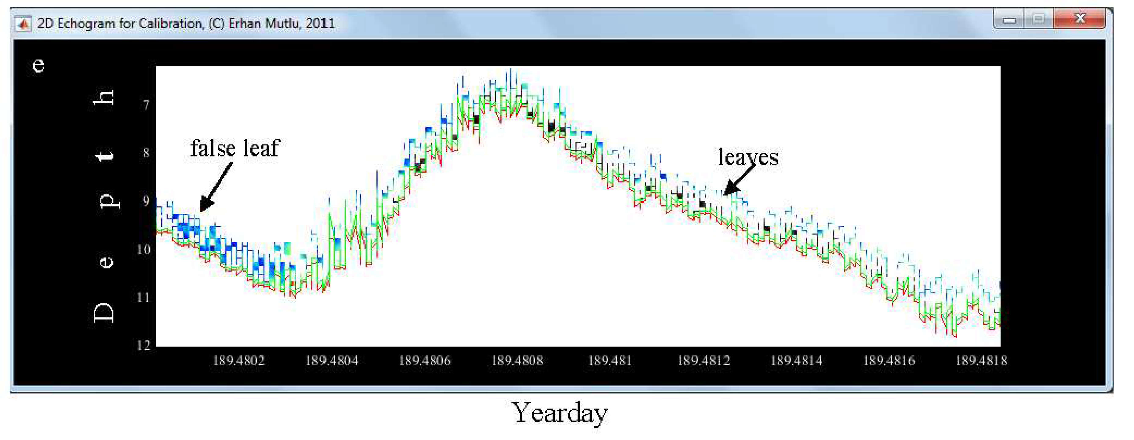
Figure 5.
Running order to estimate leaf length and biomass of the meadow in main menu, POSIBIOM.
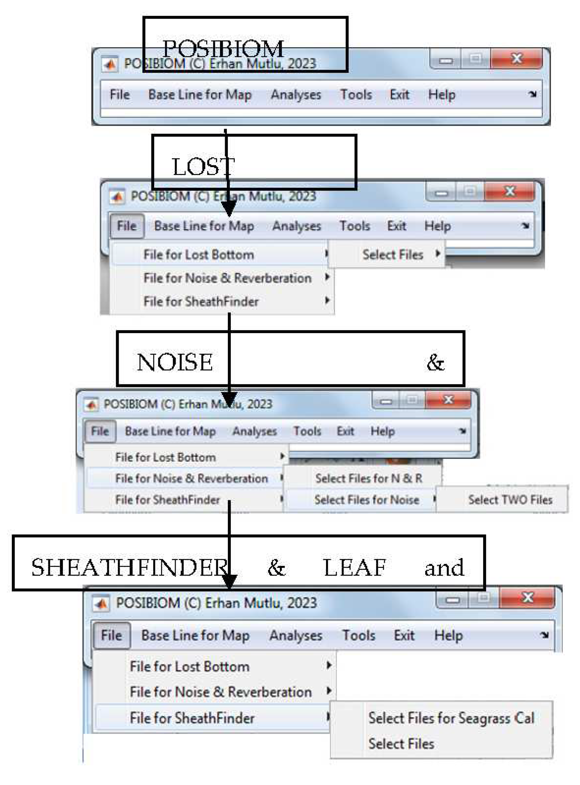
Figure 6.
The procedure followed to start the “Lost Bottom” analysis. a) Loading the coast line for map, and b) starting the analysis.
Figure 6.
The procedure followed to start the “Lost Bottom” analysis. a) Loading the coast line for map, and b) starting the analysis.
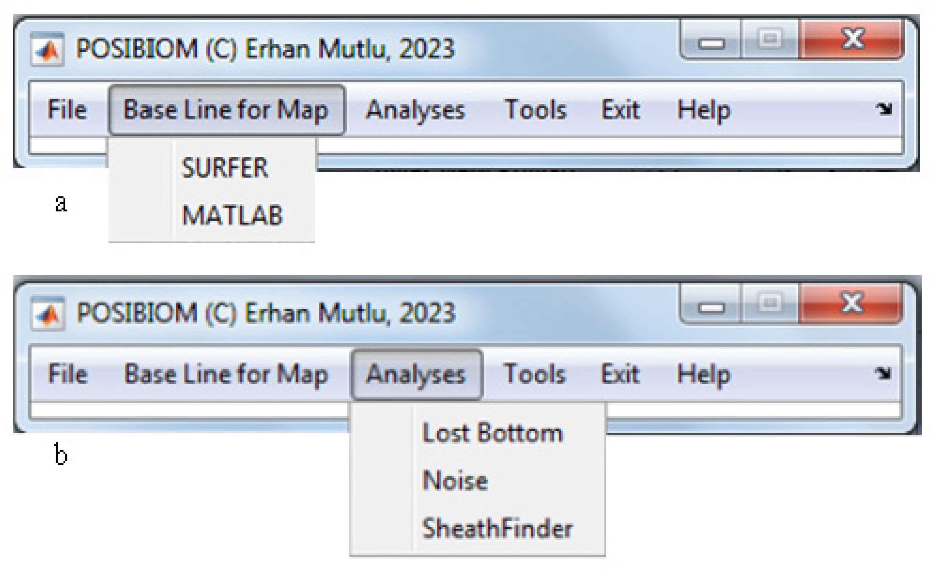
Figure 8.
Graphical outputs of the “Lost Bottom” analysis. a) Enhanced echogram before start of the analysis (green vertical lines denote the fixed lost bottom), b) an algorithm to figure out detection of the lost bottom regarding to the bottom angle and depth (blue vertical line is bottom angle, red line bottom depth), c) correction in progress after starting analysis (red vertical lines to be corrected in progress, d) bottom depth on coastal map after correction completed, e) Uncorrected bottom depth in 3D plot (vertical lineation denotes lost the bottom, e’) corrected bottom depth in 3D after finishing the analysis.
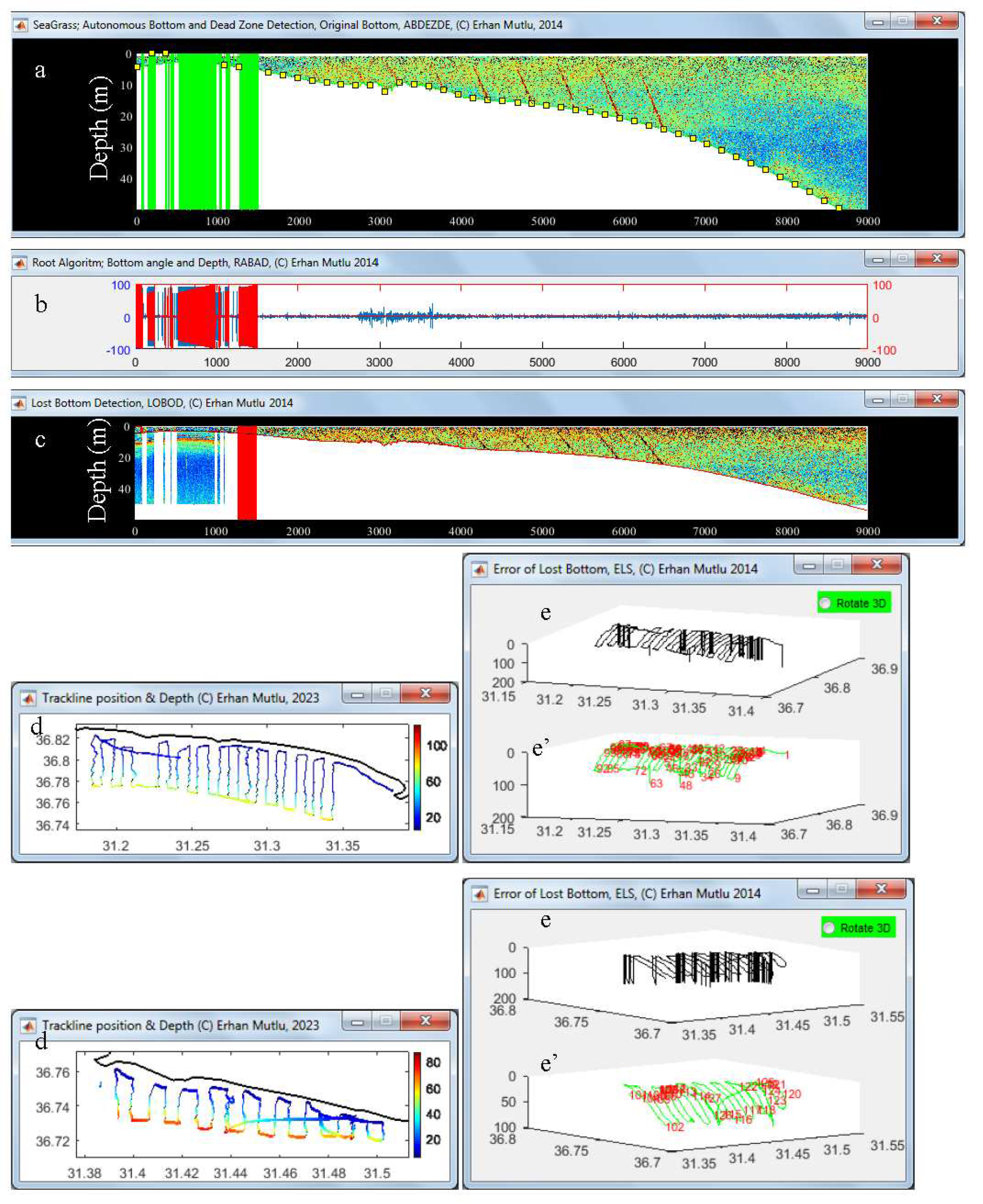
Figure 11.
Graphical menu for control, settings and info menu of “SheathFinder & Leaf and Biomass” (see Table 3 for actions of each coded option and function with number).
Figure 11.
Graphical menu for control, settings and info menu of “SheathFinder & Leaf and Biomass” (see Table 3 for actions of each coded option and function with number).
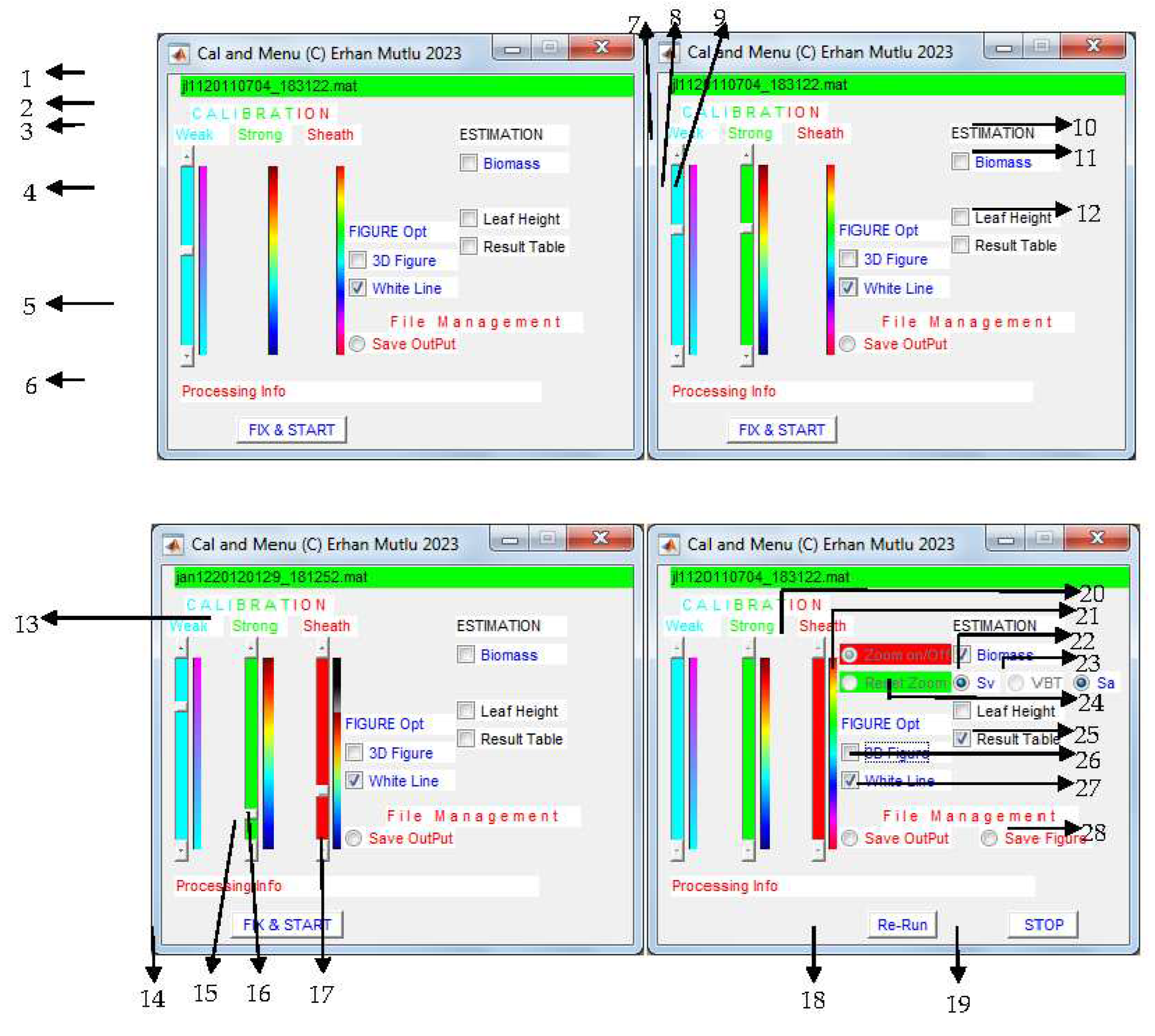
Figure 12.
Fixation and estimates of leaves of the seagrass during the analysis of the acoustical data by the “SheathFinder& Leaf and Biomass”; a) scanning sheaths or vertical rhizome by green vertical line to determine fake or real seagrass, b) estimates of the seagrass after the analysis of current file is finished (green line denotes the canopy height), and c) Result table when checking the option (option no 25 in Figure 11).
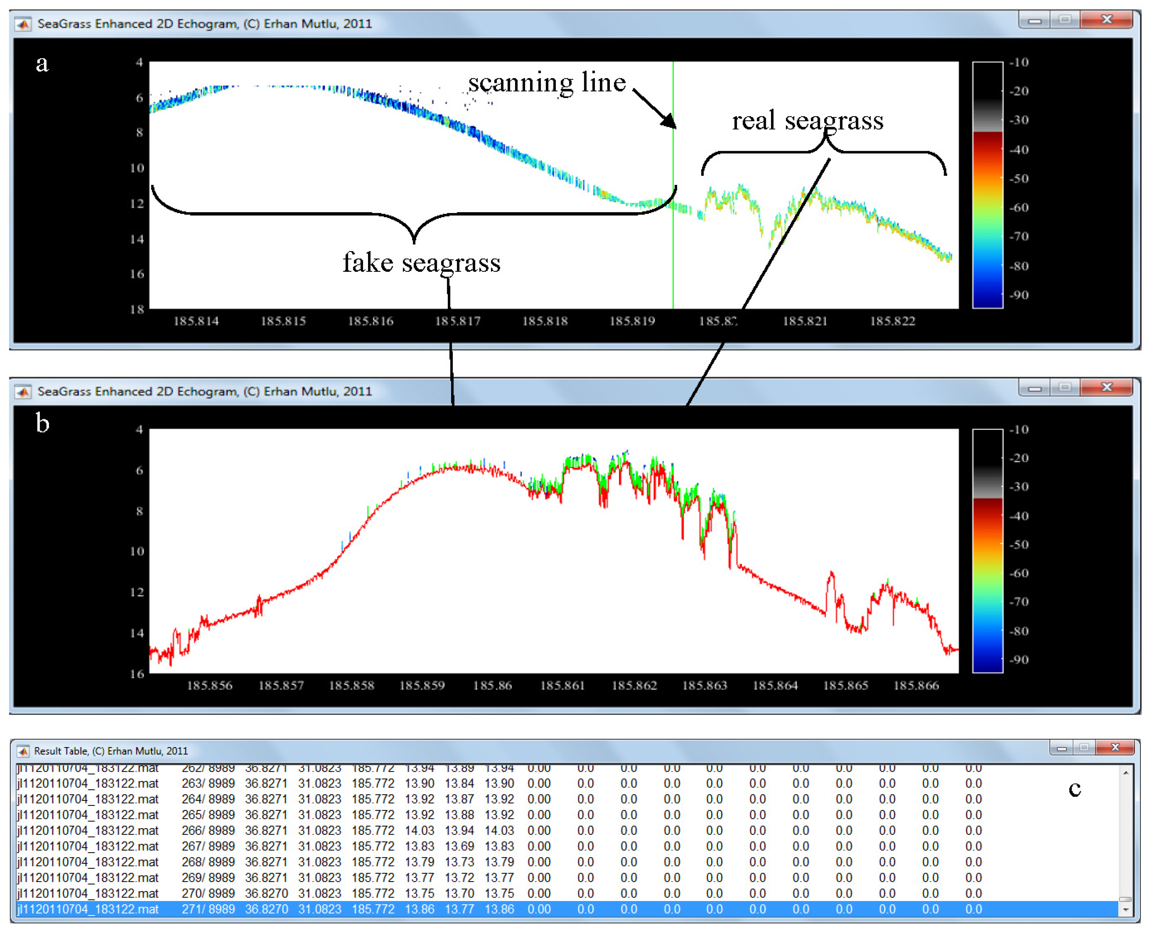
Table 1.
Fast manual to use an algorithm of “Lost Bottom” with function, if case, recommendation and Troubleshooting/negatives for each option with number (see Figure 7 for the numbers).
Table 1.
Fast manual to use an algorithm of “Lost Bottom” with function, if case, recommendation and Troubleshooting/negatives for each option with number (see Figure 7 for the numbers).
| No | Function | Case | Recommendation | Troubleshooting/negatives |
|---|---|---|---|---|
| 1 | Starting processing | First configure setting | Need to press START button after every 100 files processed | |
| 2 | Input data file name for process | |||
| 3 | Deletion of pings from the beginning | No bottom echo Bottom misestimated at the first ping |
Enter last ping no to delete | Possible to estimate wrong bottom |
| 4 | To delete the pings | Check the box | ||
| 5 | Data info of the acoustical file | Fixed during the data collection | See Appendix 4 | |
| 6 | Info for processing methods to estimate correct bottom | Auto-decision for cases (chirping, running average, filling gap) Process in cycle |
Allow auto-decision as long as possible Auto-switching to block solution in time |
Takes time; 1. for block lost bottoms 2. Single ping lost bottom in cycle |
| 7 | Transducer depth | Deployment Below surface | Required for real depth | Enter 0 if transducer at surface |
| 8 | Calibration offset | Deviation in echosounder calibration from reference ball | Acoustic data correction If less, + difference If more, - difference |
If not, uncorrected data Possible to misestimate biomass |
| 9 | Manual intervention to speed up the process | Time consuming more than usual Takes time more than 10 mins |
Step-to-step slide forward until ‘Lost bottom range’ changes (see 28) | Speed up immediately faster resulted in misestimated bottom in some case |
| 10 | ± Bottom angle | Steepness of bottom | Use default setting Too steep, adjust with bottom angle together |
Suboptimum setting detects wrong bottom |
| 11 | Bottom angle | Cliff bottom No bottom echo, too deep |
Use default setting Increase angle at highly rough sea Increase or decrease angle to estimate the deepest depth |
Strong scatterers estimated as bottom |
| 12 | Label for dead zone estimation by 3 methods | Method of the present study embedded (see Figure 1). | Obligation | Angle estimation based on ping-to-ping, not distance |
| 13 | Echo View’s dead zone | Optional, EchoView [77] |
Click for future process | Works well if GPS reports every ping |
| 14 | Alternative dead zone | Optional, Mello and Rose [78] |
Click for future process | Works well, regardless of GPS reporting every ping |
| 15 | Calculation of dead zone based on GPS coordinate distance | Disabled due to its troubleshooting | The GPS reports geographical coordinates once every one second, not every ping | |
| 16 | White line | Optional, white area between bottom depth and dead zone | optional | |
| 17 | Last check to estimate real bottom last time | Misestimated bottom still available after the process | Optional if necessary | If bottom echo is weak, change the estimated bottom completely |
| 18 | ± next bottom tracking range | Steepness of cliff bottom | Narrowing and widening the window | Jump to the strong scatterers |
| 19 | Sounding on/off the angles | Slowing the process | ||
| 20 | Saving the output data | Use for the next algorithm | optional | If step up to the next analysis, must be on |
| 21 | Saving the enhanced echogram by the corrected bottom | Optional for see the results later | Check button when user does not monitor the process | |
| 22 | Current ping range of lost bottom detected | |||
| 23 | Showing root algorithm to detect availability of lost bottom | To see goodness of the estimation of correct bottom | optional | Slowing the process |
| 24 | Current number of lost bottom detected, Loop for auto-decision of lost-bottom correction |
|||
| 25 | Showing progress status in reading the data | |||
| 26 | See 6 | |||
| 27 | See 24 | |||
| 28 | See 22 | |||
| 29 | Recovery of the real bottom (see 31, 33) from the beginning of the data to 500 pings ahead | Bottom detected too shallow or too deep | Useful for the cases | Appear after data reading complete Misrecognize the water column depth as bottom if strong scattering layer exist above the depth |
| 30 | “Chirping” method for manual intervention to recover real bottom in lost bottom range | Time consuming more than usual Takes time more than 10 mins Lost bottom range in cycle and same ping values (see 9, 22, 28) |
Useful for the cases looking at function 27, 28 in cycle | Selection of the water column depth close to the bottom if strong scattering layer exist above the depth, resulted in misestimated bottom in some case (see 32) |
| 31 | Recovery of the real bottom (see 29, 33) from the last data to 500 pings backward | Bottom detected too shallow or too deep | Useful for the cases | Appear after data reading complete Selection the water column depth close to the bottom if strong scattering layer exist above the depth |
| 32 | Water column depth for cases in 30 | Bottom detected too shallow or too deep | Useful for the cases | Appear after a certain number of iteration of the loop in function no 22, 27, but early view when sliding the speed (no 9) toward the faster, Selection of the water column depth close to the bottom if strong scattering layer exist above the depth (see 30) |
| 33 | Water column depth for recovery of the real bottom (see 29, 31) | Bottom detected too shallow or too deep | Useful for the cases | Appear after data reading complete Selection of the water column depth close to the bottom if strong scattering layer exist above the depth |
| 34 | “Filling Gap” method for manual intervention to recover real bottom in lost bottom range | Disabled | Not used currently | |
| 35 | Stopping the analysis | User stops the analysis | Do not stop if misestimating bottom depth in some data files, process again later when all files completed |
Stop after the current file processing is finished |
Table 2.
Fast manual to use an algorithm of “Noise & Reverberation” with function, case, recommendation and Troubleshooting/negatives for each option with number (see Figure 9 for the numbers).
Table 2.
Fast manual to use an algorithm of “Noise & Reverberation” with function, case, recommendation and Troubleshooting/negatives for each option with number (see Figure 9 for the numbers).
| No | Function | Case | Recommendation | Troubleshooting/negatives |
|---|---|---|---|---|
| 1 | Data file name to read | Label name | ||
| 2 | Background noise ± | label | ||
| 3 | Background noise threshold | Could adjust threshold during analysis if noise not organized well for removal | Slide up and down accordingly | Depending on background noise data measured in listening mode and signal-to-noise ratio estimated (S/N) Possible spatiotemporal changes in the noise measurements |
| 4 | ± background noise threshold for removal | threshold insufficient to detect background noise | Slide up and down to increase and decrease range of the threshold fixed (see 3) | The faster adjustment the less targets (seagrass) |
| 5 | Interference & reverberation noise ± | Label name | ||
| 6 | Interference & reverberation noise threshold | Could adjust threshold during analysis if such noise not detected well | Slide up and down accordingly | Depending on Interference & reverberation noise data measured in listening mode Spatiotemporal changes in the noise measurements |
| 7 | ± Interference & reverberation noise threshold for removal of spurious targets | threshold insufficient to detect Interference & reverberation noise | Slide up and down to increase and decrease range of the threshold fixed (see 6) | The faster adjustment the less targets (seagrass) If no noise data file for Interference & reverberation noise, background noise data file needed |
| 8 | background noise /interference & reverberation noise ratio ± | Label name | ||
| 9 | background noise /interference & reverberation ratio | Alternative method for removal such noises Could adjust threshold during analysis if noise not detected well |
Slide up and down accordingly looking at echogram | Depending on both background and Interference & reverberation noise data measured in listening mode Spatiotemporal changes in the noise measurements |
| 10 | ± background noise /interference & reverberation noise threshold for removal | threshold insufficient to detect Interference & reverberation noise | Slide up and down to increase and decrease range of the threshold fixed (see 9) | The faster adjustment the less targets (seagrass) If no noise data file for Interference & reverberation noise, background noise data file needed |
| 11 | Start analysis | Start button | After all setting done in data entry (see 12, 13) | Cannot change the data entry after functioning (see 12, 13) |
| 12 | Canopy height of seagrass | Change the default setting if necessary | First look at the canopy height at maxima in the echogram for a survey | Need a rough value, but not more than 1 m After starting analysis the entry disabled |
| 13 | Transducer depth at draft of R/V | Deployment depth below surface | Measurement for real bottom depth | Enter 0 if transducer at surface After starting analysis the entry disabled |
| 14 | info to start or stop | Label name | ||
| 15 | Info for lower limit of background S/N ratio | No detection still if correct S/N threshold set up | Use 3 and 4 in the case | Upper limit setting not independent |
| 16 | Info for background S/N ratio | No detection still if correct S/N threshold set up | Use 3 and 4 in the case | Lower and upper limit setting not independent |
| 17 | Info for upper limit of background S/N ratio | No detection still if correct S/N threshold set up | Use 3 and 4 in the case | lower limit setting not independent |
| 18 | Info for lower limit of Interference & reverberation S/N ratio | No detection still if correct S/N threshold set up | Use 6 and 7 in the case | Upper limit setting not independent |
| 19 | Info for Interference & reverberation S/N ratio | No detection still if correct S/N threshold set up | Use 6 and 7 in the case | Lower and upper limit setting not independent |
| 20 | Info for upper limit of Interference & reverberation S/N ratio | No detection still if correct S/N threshold set up | Use 6 and 7 in the case | lower limit setting not independent |
| 21 | Info for background noise /interference & reverberation S/N ratio | No detection still if correct S/N threshold set up | Use 9 and 10 in the case | Upper limit setting not independent |
| 22 | Info for background noise /interference & reverberation S/N ratio | No detection still if correct S/N threshold set up | Use 9 and 10 in the case | Lower and upper limit setting not independent |
| 23 | Info for upper limit of background noise /interference & reverberation S/N ratio | No detection still if correct S/N threshold set up | Use 9 and 10 in the case | lower limit setting not independent |
| 24 | Stopping the analysis | User wants to stop the analysis | Do not stop if misestimated noise removal in some data files, process that later again when all files completed |
Stop after the current file processing, not immediately |
| 25 | Dead Zone and methods | Label name | ||
| 26 | Dead zone estimated by the present study | Optional, Present study, |
Click on to involve that into average Dead Zone calculation, or not | Angle estimation based on ping-to-ping, not distance, Need to include the most precise methods of dead zone for average, At least one of three methods required for the next analysis |
| 27 | Echo View’s dead zone | Optional, EchoView [77] |
If available in the input data, option enable | Works well if GPS reports every ping, At least one of them required for the next analysis |
| 28 | Alternative dead zone | Optional, Mello and Rose [78] |
If available in the input data, option enable | Works well, regardless of GPS reporting every ping, At least one of them required for the next analysis |
| 29 | Data management to save output data, or figure, or to show S/N solution figures | Label name | ||
| 30 | Saving the enhanced echogram by the corrected bottom | Optional to see the results later | Check button when user does not monitor the process | |
| 31 | Saving the processed data | Use for the next algorithm | optional | If stepping to the next analysis, must be on |
| 32 | Only S/N solution figures | To show the figures | optional | Slow down the analysis |
Table 3.
Fast manual to use an algorithm of “SheathFinder & Leaf and Biomass” with function, case, recommendation and Troubleshooting/negatives for each option with number (see Figure 11 for the numbers).
Table 3.
Fast manual to use an algorithm of “SheathFinder & Leaf and Biomass” with function, case, recommendation and Troubleshooting/negatives for each option with number (see Figure 11 for the numbers).
| No | Function | Case | Recommendation | Troubleshooting/negatives |
|---|---|---|---|---|
| 1 | Current input file name on process | Updating by file to file | ||
| 2 | Title for removal of spurious weak and strong scatterers, and sheaths | label | ||
| 3 | Label of weak scattering removal | label | ||
| 4 | Calibration threshold setting to remove weak scatterers | High background noise, some weak zooplankton layers | Adjust neither less nor more looking at the enhanced echogram | A good calibration data for showing clear seagrass |
| 5 | Color scale to guide user to slide up or down for weak scatterers removal | colorbar | Colors cannot fit to the acoustical data echogram in some cases, looking at the echogram | |
| 6 | current info while processing the data | Strong scattering removal takes time | ||
| 7 | Label of strong scattering removal | label | ||
| 8 | Calibration threshold setting to remove strong scatterers | Reverberation, interference, Fishes and schools, compact zooplankton layers | Adjust neither less nor more looking at the enhanced echogram | A good calibration data needed for showing clear seagrass, appears after function 4 completed |
| 9 | Color scale to guide user to slide up or down for strong scatterers removal | colorbar | Colors cannot fit to the acoustical data echogram in some cases, looking at the echogram | |
| 10 | Title to show results in figure and table of the estimation | label | ||
| 11 | Showing figure for estimated biomass on map with trackline | Optional, | Use “tools” after the analysis completed | Slowing the analyses, trackline width constant |
| 12 | Showing figure for estimated leaf (canopy) length on map with trackline | Optional, | Use “tools” after the analysis completed | Slowing the analyses, trackline width constant |
| 13 | Label of sheaths fixation and removal | label | ||
| 14 | Fixing the settings and then start the analysis | All settings completed | Functions in 20 and 21 will be disabled after the start, Press START button after every 100 files processed |
|
| 15 | Calibration threshold setting to fix and remove the sheath | Calibration to fix sheath threshold | Adjust neither less nor more looking at the enhanced echogram until sheath disappear, Fix threshold ligule if sheath too short in time, use functions 20 and 21, if not well fixing settings, restart from function 4 |
A good calibration data needed for showing clear seagrass with sheaths, too short sheath could not be detected in time of year, appears after function 8 completed |
| 16 | Color scale to guide user to slide up or down for fixing and removing sheath | colorbar | Colors cannot fit to the acoustical data echogram in some cases, looking at the echogram | |
| 17 | Saving outputs into file in *.xls format | For mapping the biomass and canopy height later | Use the” tools” or other mapping software | Three different biomass estimation, some could be different from each other |
| 18 | Re-start the analysis from the beginning | Not well works for the estimates | Use the option when case needed | All settings needed from the beginning |
| 19 | Stopping the analysis | User stops the analysis | Use in case of function 18 | Stop after the current file completed, not immediately |
| 20 | Zooming on the main echogram | Fixing sheaths better for large file | Use the options | No way for zoom back to previous appearance, Use function 19, Disabled after starting analysis |
| 21 | Zoom back to original size of the echogram | To select better sheaths on the echogram | Use the option when case needed | Disabled after starting analysis |
| 22 | Method VBT to estimate biomass | Disabled | Need of the VBT software | |
| 23 | Method to map estimate biomass based on Sa | Only estimates using regression between biomass and Sa | use if necessary | Slowing down the processing, appear only after checking function 11, Estimates (Sa and Sv) always available in the output file |
| 24 | Method to map estimate biomass based on Sv | Only estimates using regression between biomass and Sv | Use if necessary | Slowing down the processing, appear only after checking function 11, Estimates (Sa and Sv) always available in the output file |
| 25 | Show the complex estimates with many variables in a scrolling Table | optional | optional | Slowing down the processing, Click off/on not to show the results |
| 26 | Show 3D curtain enhanced echogram | optional | optional | Slowing down the processing, |
| 27 | White line on 2D echogram | Optional, white area between bottom depth and dead zone | optional | Not in 3D echogram |
| 28 | Save figures for mapping biomass or leaf height | When function 11 or 12 checked, respectively or both | Optional, use the “tools” or other mapping software later | Saving after finishing all files processing, see function 11 and 12, appear only after checking function 11 or 12 |
Disclaimer/Publisher’s Note: The statements, opinions and data contained in all publications are solely those of the individual author(s) and contributor(s) and not of MDPI and/or the editor(s). MDPI and/or the editor(s) disclaim responsibility for any injury to people or property resulting from any ideas, methods, instructions or products referred to in the content. |
© 2023 by the authors. Licensee MDPI, Basel, Switzerland. This article is an open access article distributed under the terms and conditions of the Creative Commons Attribution (CC BY) license (http://creativecommons.org/licenses/by/4.0/).
Copyright: This open access article is published under a Creative Commons CC BY 4.0 license, which permit the free download, distribution, and reuse, provided that the author and preprint are cited in any reuse.


