
Submitted:
18 June 2023
Posted:
19 June 2023
You are already at the latest version
Abstract
Road intersections are made of asphalt pavement, a popular road surface material used worldwide. The pavement may suffer deformities and deterioration, resulting in higher maintenance expenses and an elevated likelihood of road accidents, due to factors such as heavy vehicles and environmental variables like temperature and rainfall. To tackle these obstacles, researchers have devised several machine-learning algorithms and optimization techniques. These tools aim to forecast and scrutinize pavement deformation, with the goal of refining pavement design and maintenance approaches, as well as obtaining a more comprehensive comprehension of the factors that impact pavement effectiveness. This paper shows that heavy vehicles contribute significantly more to road erosion, and the retention and braking of vehicles greatly impact roadways. We also emphasize the statistical errors computed on the actual data range and demonstrate the results of the multilayer perceptron (MLP) model. The MLP model used the lath erosion standard to simulate future impact. Even though the model given is based on a small sample of data from one intersection, its estimates for road erosion in a year were found to be accurate when contrasted to real data. Controlling traffic flow can significantly improve road conditions, reducing erosion decay by reducing the time spent at intersections and other parameters. We conclude that machine learning can help control traffic flow, which can significantly improve road conditions, reducing vehicle time stretches at intersections.
Keywords:
Regression
; Modeling erosion coefficients
; Simulation
; Back propagation
; Lath and nail method
1. Introduction
The study of the impact of traffic flow on the deformation of asphalt surfaces is an important research area in transportation engineering. Understanding how vehicles affect asphalt deformation can aid in the development of more durable and cost-effective roadways. Road degradation depends on traffic flow.
Current road construction is based on solid calculations, including weather conditions, the number of vehicles, etc. These calculations generally assume a minimum road lifespan of 10 years, which can go up to 35 years. This research has shown, however, that we cannot assume this calculation is correct because intersections can alter traffic flow, which in turn influences road erosion. This study models, maps, and correlates the connection between traffic flow and road erosion using data from a single intersection. According to the findings, ten years may not even be the absolute minimum that a road segment at an intersection can expect to last. The model relies heavily on traffic flow parameters but ignores environmental factors like temperature and humidity because it only considers a single junction and a small amount of data.
To study this phenomenon, data from videos was extracted and processed to acquire real-time vehicle movement and asphalt impact data. Following that, patterns and correlations between traffic flow and asphalt deformation can be found by analyzing the data using computational algorithms, such as the backpropagation algorithm. Additionally, analyzing this data can help identify critical factors that affect asphalt deformation and assist in developing predictive models to estimate asphalt's lifespan. The results of this research are modeled using machine learning (ML) technique with the previously mentioned limitations.
The outline of the research is as follows: The introduction and review of literature offer a concise summary of the existing research in this field. The methods used to calculate erosion rates in the future are outlined in the methodology section. Using the proposed models, the results section summarizes the research findings and discusses their implications. Lastly, the conclusion gives specific ideas and directions for future study.
2. Materials and Methods
Asphalt pavement deformation, particularly rutting deformation, is a major concern in the transportation industry due to its adverse effects on road safety and performance. Numerous studies have been carried out in order to gain an understanding of the underlying causes and make predictions regarding the deformation that big vehicle loads will have on asphalt surfaces. One of which is a prediction model for asphalt pavement deformation using artificial neural networks. The model considered various environmental factors, such as temperature and rainfall, in addition to traffic volume. The model accurately predicted heavy vehicle load asphalt pavement deformation [1,2]. Laboratory tests examined asphalt's rutting deformation under heavy-load vehicles [3]. Tire pressure and axle load impacted rutting. Axle load and tire pressure affected asphalt pavement rutting, according to the findings.
Similarly, [4] presented a prediction model for asphalt pavement deformation using an artificial neural network. Different data parameters were used to train and validate the model. Results indicated that the model was able to accurately predict the deformation of asphalt pavement under heavy vehicle loads. The support vector machine (SVM) optimized using a genetic algorithm (GA) and created by [5] predicts asphalt pavement rutting based on field test data and was evaluated using mean absolute error, root mean square error, and correlation coefficient. The model accurately predicted asphalt pavement rutting. Likewise, [6] investigated asphalt pavement deformation using a genetic algorithm optimized back-propagation neural network. Root mean square error and correlation coefficient were used to evaluate the field test-based model. The findings proved that the model accurately predicted the deformity of asphalt pavement.
[7,8] investigated the relationship between traffic flow and asphalt deformation using video data extraction and processing. The study analyzed the data with a back-propagation algorithm to determine the impact of traffic flow on asphalt deformation. Findings indicated that traffic flow significantly affected asphalt deformation, and the model had good accuracy in predicting the deformation. Finally, [9,10] studied the effects of vehicle speed on rutting deformation of asphalt pavement using real-time traffic data. The study used a regression analysis to identify the relationship between vehicle speed and rutting deformation. Deformation caused by rutting was found to be significantly affected by vehicle speed.
The Yong study analyzed the effects of graphene on asphalt's performance and the effectiveness of sma in pavement. Based on a Gansu Province highway project, graphene enhanced asphalt was used [11]. To prepare CRCM asphalt, which includes CRCM-SBS, CRCM-Sasobit/BRF, and CRCM-RARX, the same amount of crumb rubber and various amounts of composite additives were added [12]. Long-term road performance is assessed and predicted for self-ice-melting asphalt surfaces equipped with salt-storage materials in this lab study [13]. Employing Dynamic Mechanical Analysis, Ma tested three variations of an asphalt mixture used for the surface course and six standard RIOHTrack structures [14]. Xiao proposes a new fatigue life prediction that takes temperature load into account [15], which could be disregarded in inspections of steel deck welds on suspension bridges subjected to dynamic vehicle load. Liu makes use of the data that is reflective of the weather for a period of twenty-four hours during the summer [16]. Two-dimensional image technology obtains air-void data acquired from rutting sample sections with varied loading cycles (500, 1000, 1500, 2000, 2500, and 3000 times) [17]. Wu intends to conduct a comprehensive investigation to determine the law of skid resistance attenuation of SMA pavement [18]. Langa examines how high-density polyethylene (HDPE) modified asphalt binder changes in terms of its physical, rheological, and thermal properties after soybean oil is added [19].
To aid in the right decision-making processes, a long-term strategy for pavement preservation should include a thorough evaluation of the current road state. To predict flexible pavements' durability over time, [20] puts forward integrating Non-Destructive Testing (NDT) and ground truth data. Shaffie proves RSM's statistical efficacy [21]. Cao simulates the thermodynamic, diffusion, and adhesion effects of asphalt cement aging using molecular dynamics [22]. [23] carried out a model-based farm-scale exploratory study using two farms as case studies. In [24], researchers looked at 15 extracts from the peels of 5 different cultivars to determine their phytochemical makeup, antioxidant activity, tyrosinase influence, in vitro SPF, and cytotoxicity. As the service life increases, the actual load-carrying capacity of bridges gradually decreases due to the combined action of the environmental corrosion and repeated vehicle loads, resulting in shortened bridge service life. Nie study fatigue reliability analysis and traffic load control of steel bridges based on artificial neural network [25]. The fatigue reliability index of a steel girder bridge over its whole life is investigated based on artificial neural networks. Hussein wants to emphasize the significance of planning marsh management, which may revitalize the marshes' natural world before drying through the Center for Marsh Revitalization in southern Iraq [26]. Cepa presents the main types of sensors and their applications in tunnels [27]. Assessing pavement condition effectively helps with making good decisions and provides longer-lasting pavement mixes, as discussed in [28].
3. Methodology
Traffic flow's effect on road conditions is the study's main objective. Machine learning algorithms are used to analyze and simulate traffic flow data. In order to measure different types of asphalt erosion or decay a different measuring method can be applied [29]. Research results focus on the lath and nail method and future erosion coefficient will be lath and nail method related. For the lath and nail method, the changes in the pavement are measured by using an aluminum lath that is 4 meters in length. Typically, they have a rectangular cross-section and are made of solid wood or light metal, leaving no room for speculation. It is crucial that the measuring lath has no fewer than two supports. Figure 1 displays a sand patch and lath-and-nail method.
Samples and data are collected at the intersection of roads M223 and R363 near Tuzla, Bosnia and Herzegovina. The data is collected at the crossing point entrance from Tuzla city side where black-top thickness layers are 7cm and 5cm where the 5 cm layer is the best one liable for connection with the tire while the other one is obligated for the heap pressure taking care of, also the path width given to be 2.75 m and the black-top blend qualities given as BB11s for the top layer and AGNS 22sA for the base layer with the tampon thickness given in reach from 31 to 40 cm. For this location, the traffic flow data is obtained from two different sources.
First source is a video document source using road surveillance cameras with a 15-day period, which was used for sampling. A linear support vector machine model extracts vehicle number, class, speed, heading, and time from the recorded footage [8]. The weather and temperature factors are not considered as the measurements and modeling is performed on nearby lanes. Figure 2 depicts the detection of on-road vehicles in an area of interest, a key data collection point [8]. HOG and SVM gather data in the region of interest. HOG data includes boundaries from vehicle-free and vehicle-present images.
Positive set is a region of interest with identified vehicles excluded from source recordings., likewise the negative set is no vehicles from roads, structures, etc. 2954 images of vehicles make up the positive training set. The negative training set has 2860 vehicle-free images. A 64x64 pixel resolution is applied to these images. We count the number of directions in each square. Find more than 9 directions. Each square has 8 pixels that show us which way things are pointing. We create histograms with 2 squares for every larger square. This results in a new, smaller image that depicts the various directions in the original image. It has a size of only 16 by 16 pixels.
HOG descriptor, spatial picture vector, and situated angles histogram make up element vector. With given details, a Linear SVM can precisely identify objects of significance and those that are not. 70% and 30% of the train and test sets received the new vector. The utilized clip sets have 98-100% precision [8].
As mentioned before from the video data, we have identified breakdown of vehicle’s type, time, travel direction and stopping action at the intersection for the 15-day period.
Second source of traffic data is governmental sensor flow data between 10/26/2015-06/12/2020. The actual sensor flow measurements are taken on the main Tuzla-Sarajevo Freeway. The data contains type, number of vehicles, and direction of travel.
The input dataset is created by combining video data with traffic department sensor data and road erosion measurements as follows:
- Number of LW vehicles—The complete count of light vehicles (LW) for a given interval;
- HW vehicle count—The overall count of heavy vehicles (HW) for a particular period;
- Date range (h)—From 27.10.2015 to 12.06.2020, inclusive, to determine specified intervals;
- Time on the intersection/junction (h) for HW—Determined from footage data averages and multiplied by the total number of (HW) vehicles;
- Time on the intersection/junction (h) for LW—The total count of (LW) vehicles multiplied by the average value derived from video data;
- Number of HW that are coming to a full stop—Calculated with respect to the percentage amount;
- Road erosion (lath)— Machine learning models use percentage assumptions;
Daily datasets are created for the two road intersection lanes. This study ignores weather and temperature because the lanes are adjacent. The total amount of records that comprise the final data set is 3382 days across the two lanes. Table 1 shows examples of the dataset based on daily left lane traffic flow [9].
With Lath measurement of 60 mm in 2020 used as output parameter, we have applied machine learning/ regression methods to develop a model for erosion coefficient prediction. Assuming linear decay, we have trained the model to associate the vehicle behavior to road decay over time. We used decision tree, linear, random forest, and gradient boosting regression models [9].
As explained before the aim of research is to measure that impact by combining experimental and theoretical data sets and to apply machine learning methods (ML) or neural networks which are basic versions similar to a human brain that involve input, hidden and output layers. Our objective is to generate meaningful outputs for a provided input. After implementing different ML methods, which were tested out, results have shown that the multilayer-perceptron-back propagation algorithm was able to correlate input and output data parameters [9]. The most common neural network approach is called a multi-layer perceptron (MLP). The neurons and hidden layer are arranged such that in each layer, the nodes only get inputs from the nodes in the previous layer and only send their outputs to the nodes in the next layer [30]. The input data set is traffic flow, and the output is road erosion. After running different error matrices, the MLP model was confirmed to be accurate and was used for future road erosion prediction. Throughout training, the MLP learns to recognize input-output correlations. MLP can learn a non-linear regression approximation from input variables and a target or output value. Figure 3 illustrates an MLP framework with a single concealed layer.
The left side displays a set of input parameters denoted by x that are actually elements from Table 1. On-road degradation measured by lath-nail technique is the target value or Y(x). The hidden layer weights are recalibrated through the process of determining the amount by which the target values differ from the predicted values.
3. Results and Discussion
Erosion of roads and how it affects the flow of traffic are discussed. The predicted "lath" measurements are put forward in this paper. Figure 4 depicts the MLP model's prediction for the "lath" dataset set compared to the actual statistical value.
The test stage includes 30 % of the dataset, the calculation of the overall test set average absolute difference is 4.88 %, R2=0.9948 and (Mean squared error) MSE=0.00042. Enhancements to the model are range- and size-dependent.
Figure 4 presents a prediction based on the normalized and linearized samples. The MLP projections use a dataset that has been arbitrarily divided into 70% training data and 30% testing data. Stochastic gradient descent is used for optimization, and the back-propagation algorithm is used for learning in the MLP model, with square error as the loss function. Table 2 gives a sample of test set. Last column (Predicted value) shows MLP results so we can compare to measured/statistical values (Road erosion (lath). MLP takes rest of the table as input.
MLP prediction is accurate because predicted and measured values match. Heavy vehicles erode roads, as shown.
In Table 3, we show the result from right lane learned data set, meaning based on trained MLP model, we input new data points to understand the underlying impact of different inputs.
Actual measurement of road erosion (lath) 4.6 years after road is completed is 60 mm. The limitations are related to the dataset as only data from one intersection was used for modeling. Traffic can drastically alter street conditions. Using AI, we can predict the erosion and significantly improve control of the traffic flow to optimize road erosion due to the traffic. The real test uses measurements from the 2nd intersection. The introduction to a new intersection data is the next step before the model is applied. The "Lath" measurement can be seen in Figure 5.
With the "Lath" standards reading equal to 16 mm. The "Lath" standards reading can be confirmed from the Figure 5 and at the back the "Sand" measurements can be seen too.
In Figure 6, intersections sketch is provided with indicated points of observations.
All the measurements are summarized in Table 4, and all of them are for T1 location.
Both Table 4 input parameters are derived from traffic/statistical data, and the time interval is identical to that of the initial intersection. Table 4's first two parameters determine the next three parameters. Since the first intersection was observed at 25 m and the second at 75 m, the values have to be considerably smaller than those from the first intersection. MLP Road erosion (lath) model prediction is 16.62 mm.
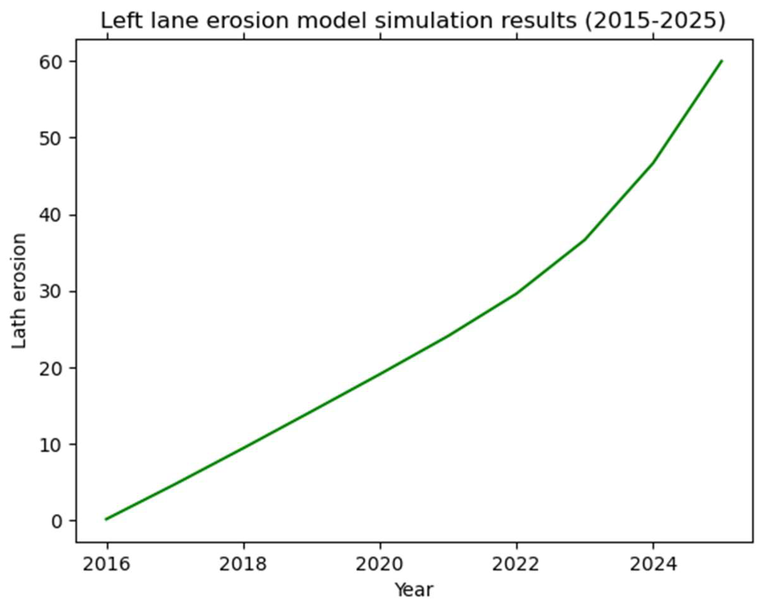
Finally, MLP that learned from right lane is used to predict the behavior in the left lane. This impact is shown in Table 5 and Figure 8 and lane left lane location is shown in Figure 7 as T2 point.
The following inputs for heavy and light vehicles are calculated by applying the known spectrum of past years which is later used to calculate the number of vehicles in the future. Other input variables are calculated with respect to the average and percentage values for the left lane which is explained in detail before.
5. Conclusions
As AI and image processing technology improve, future research in engineering will have access to new data and research fields will arise. This research measures the impact and suggests ways to make way roads safer and last longer. We studied the impact of heavy vehicles on road erosion at a specific intersection in Bosnia and Herzegovina. The study found that vehicle retention and braking affect roadways greatly, but there are limitations to the study based on the amount of data used, the lack of weather data, and the use of civil engineering measurements. The study suggests the need for more research on traffic flow control and its impact on road conditions, as well as the impact of climate and vehicle gas consumption on road development planning. Additionally, future research could explore the impact of smart traffic flow solutions on road conditions.
Author Contributions
Conceptualization, Sabahudin Vrtagic and Edis Softic; methodology, Sabahudin Vrtagic.; software, Sabahudin Vrtagic.; validation, Sabahudin Vrtagic, Fatih Dogan and Milan Dordevic; formal analysis, Muhammed Codur; investigation, Mario Hoxha.; resources, Mario Hoxha.; data curation, Sabahudin Vrtagic.; writing—original draft preparation, Sabahudin Vrtagic.; writing—review and editing, Fatih Dogan and Mario Hoxha.; visualization, Sabahudin Vrtagic; supervision, Sabahudin Vrtagic; project administration, Sabahudin Vrtagic and Mario Hoxha. All authors have read and agreed to the published version of the manuscript.
Funding
This research received no external funding.
Conflicts of Interest
The authors declare no conflict of interest.
References
- Keskin, M.; Karacasu, M. Artificial Neural Network Modelling for Asphalt Concrete Samples with Boron Waste Modification. Journal of Engineering Research 2021. [CrossRef]
- Zhang, Q.; Chen, Y.; Li, X. Rutting in Asphalt Pavement under Heavy Load and High Temperature. Asphalt Material Characterization, Accelerated Testing, and Highway Management 2009. [CrossRef]
- Nian, T.; Li, J.; Li, P.; Liu, Z.; Guo, R.; Ge, J.; Wang, M. Method to Predict the Interlayer Shear Strength of Asphalt Pavement Based on Improved Back Propagation Neural Network. Construction and Building Materials 2022, 351, 128969. [Google Scholar] [CrossRef]
- Issa, A.; Samaneh, H.; Ghanim, M. Predicting Pavement Condition Index Using Artificial Neural Networks Approach. Ain Shams Engineering Journal 2022, 13, 101490. [Google Scholar] [CrossRef]
- Nguyen, H.-L.; Le, T.-H.; Pham, C.-T.; Le, T.-T.; Ho, L.S.; Le, V.M.; Pham, B.T.; Ly, H.-B. Development of Hybrid Artificial Intelligence Approaches and a Support Vector Machine Algorithm for Predicting the Marshall Parameters of Stone Matrix Asphalt. Applied Sciences 2019, 9, 3172. [Google Scholar] [CrossRef]
- Reza Kashyzadeh, K.; Amiri, N.; Ghorbani, S.; Souri, K. Prediction of Concrete Compressive Strength Using a Back-Propagation Neural Network Optimized by a Genetic Algorithm and Response Surface Analysis Considering the Appearance of Aggregates and Curing Conditions. Buildings 2022, 12, 438. [Google Scholar] [CrossRef]
- Chang, Y.; Wang, Y.; Sun, C.; Zhang, P.; Xu, W. Day-to-Day Dynamic Traffic Flow Assignment Model under Mixed Travel Modes Considering Customized Buses. Sustainability 2023, 15, 5440. [Google Scholar] [CrossRef]
- Vrtagić, S.; Softić, E.; Ponjavić, M.; Stević, Ž.; Subotić, M.; Gmanjunath, A.; Kevric, J. Video Data Extraction and Processing for Investigation of Vehicles’ Impact on the Asphalt Deformation Through the Prism of Computational Algorithms. Traitement du Signal 2020, 37, 899–906. [Google Scholar] [CrossRef]
- Vrtagić, S. et al. Traffic Flow Influence on the Bitumen Distortion Through the Back Propagation Algorithm Based on the Real on Road Formed Dataset Parameters. In: Ademović, N., Mujčić, E., Akšamija, Z., Kevrić, J., Avdaković, S., Volić, I. (eds) Advanced Technologies, Systems, and Applications VI. IAT 2021. Lecture Notes in Networks and Systems, vol 316. Springer, Cham. [CrossRef]
- Khan, M.I.; Ullah, H.; Khan, K.M.; Khan, K.; Arifuzzaman, Md. EVALUATION OF SPEED EFFECT OF VEHICLES ON ASPHALT PAVEMENT. Proceedings of International Structural Engineering and Construction 2015, 2. [Google Scholar] [CrossRef]
- Kotek, P.; Kováč, M. Comparison of Valuation of Skid Resistance of Pavements by Two Device with Standard Methods. Procedia Engineering 2015, 111, 436–443. [Google Scholar] [CrossRef]
- Yong, P.; Tang, J.; Zhou, F.; Guo, R.; Yan, J.; Yang, T. Performance Analysis of Graphene Modified Asphalt and Pavement Performance of SMA Mixture. PLOS ONE 2022, 17, e0267225. [Google Scholar] [CrossRef]
- Gong, F.; Lin, W.; Chen, Z.; Shen, T.; Hu, C. High-Temperature Rheological Properties of Crumb Rubber Composite Modified Asphalt. Sustainability 2022, 14, 8999. [Google Scholar] [CrossRef]
- Ansar, M.; Sikandar, M.A.; Althoey, F.; Tariq, M.A.U.R.; Alyami, S.H.; Elsayed Elkhatib, S. Rheological, Aging, and Microstructural Properties of Polycarbonate and Polytetrafluoroethylene Modified Bitumen. Polymers 2022, 14, 3283. [Google Scholar] [CrossRef] [PubMed]
- Zhang, H.; Guo, R. Investigation of Long-Term Performance and Deicing Longevity Prediction of Self-Ice-Melting Asphalt Pavement. Materials 2022, 15, 6026. [Google Scholar] [CrossRef] [PubMed]
- Ma, Z.; Wang, X.; Wang, Y.; Zhou, X.; Wu, Y. Long-Term Performance Evolution of RIOHTrack Pavement Surface Layer Based on DMA Method. Materials 2022, 15, 6461. [Google Scholar] [CrossRef] [PubMed]
- Xiao, X.; Zhang, H.; Li, Z.; Chen, F. Effect of Temperature on the Fatigue Life Assessment of Suspension Bridge Steel Deck Welds under Dynamic Vehicle Loading. Mathematical Problems in Engineering 2022, 2022, 1–14. [Google Scholar] [CrossRef]
- Liu, P.; Kong, X.; Du, C.; Wang, C.; Wang, D.; Oeser, M. Numerical Investigation of the Temperature Field Effect on the Mechanical Responses of Conventional and Cool Pavements. Materials 2022, 15, 6813. [Google Scholar] [CrossRef] [PubMed]
- Zhao, K.; Yang, H.; Wang, W.; Wang, L. Characterization of Rutting Damage by the Change of Air-Void Characteristics in the Asphalt Mixture Based on Two-Dimensional Image Analysis. Materials 2022, 15, 7190. [Google Scholar] [CrossRef]
- Gkyrtis, K.; Plati, C.; Loizos, A. Mechanistic Analysis of Asphalt Pavements in Support of Pavement Preservation Decision-Making. Infrastructures 2022, 7, 61. [Google Scholar] [CrossRef]
- Shaffie, E.; Jaya, R.P.; Ahmad, J.; Arshad, A.K.; Zihan, M.A.; Shiong, F. Prediction Model of the Coring Asphalt Pavement Performance through Response Surface Methodology. Advances in Materials Science and Engineering 2022, 2022, 1–17. [Google Scholar] [CrossRef]
- Cao, W.; Fini, E. A Molecular Dynamics Approach to the Impacts of Oxidative Aging on the Engineering Characteristics of Asphalt. Polymers 2022, 14, 2916. [Google Scholar] [CrossRef]
- Aguerre, V.; Chilibroste, P.; Casagrande, M.; Dogliotti, S. Exploring Alternatives for Sustainable Development of Mixed Vegetable Beef-Cattle Family Farm Systems in Southern Uruguay. Agrociencia Uruguay 2022, 26. [Google Scholar] [CrossRef]
- Ansar, M.; Sikandar, M.A.; Althoey, F.; Tariq, M.A.U.R.; Alyami, S.H.; Elsayed Elkhatib, S. Rheological, Aging, and Microstructural Properties of Polycarbonate and Polytetrafluoroethylene Modified Bitumen. Polymers 2022, 14, 3283. [Google Scholar] [CrossRef] [PubMed]
- Gaweł-Bęben, K.; Czech, K.; Strzępek-Gomółka, M.; Czop, M.; Szczepanik, M.; Lichtarska, A.; Kukula-Koch, W. Assessment of Cucurbita Spp. Peel Extracts as Potential Sources of Active Substances for Skin Care and Dermatology. Molecules 2022, 27, 7618. [Google Scholar] [CrossRef] [PubMed]
- Czarnecki, A.A.; Nowak, A.S. Time-Variant Reliability Profiles for Steel Girder Bridges. Structural Safety 2008, 30, 49–64. [Google Scholar] [CrossRef]
- Moharekpour, M.; Liu, P.; Oeser, M. Evaluation and Improvement of the Current CRCP Pavement Design Method. Materials 2022, 16, 358. [Google Scholar] [CrossRef] [PubMed]
- Hussein, A.A.K.; Asal, A.A. Drying Water and Its Impact on the Vital System in the Marshes of Southern Iraq. IOP Conference Series: Earth and Environmental Science 2023, 1129, 012032. [Google Scholar] [CrossRef]
- Ergun, M.; Iyinam, S.; Iyinam, A.F. Prediction of Road Surface Friction Coefficient Using Only Macro- and Microtexture Measurements. Journal of Transportation Engineering 2005, 131, 311–319. [Google Scholar] [CrossRef]
- Pedregosa, F.,et. al., Scikit-learn: Machine Learning in Python, Journal of Machine Learning Research, vol. 12, pp. 2825–2830, 2011. arXiv:1201.0490.
Figure 1.
Visualizing data collection with sand patch and lath/nail method.
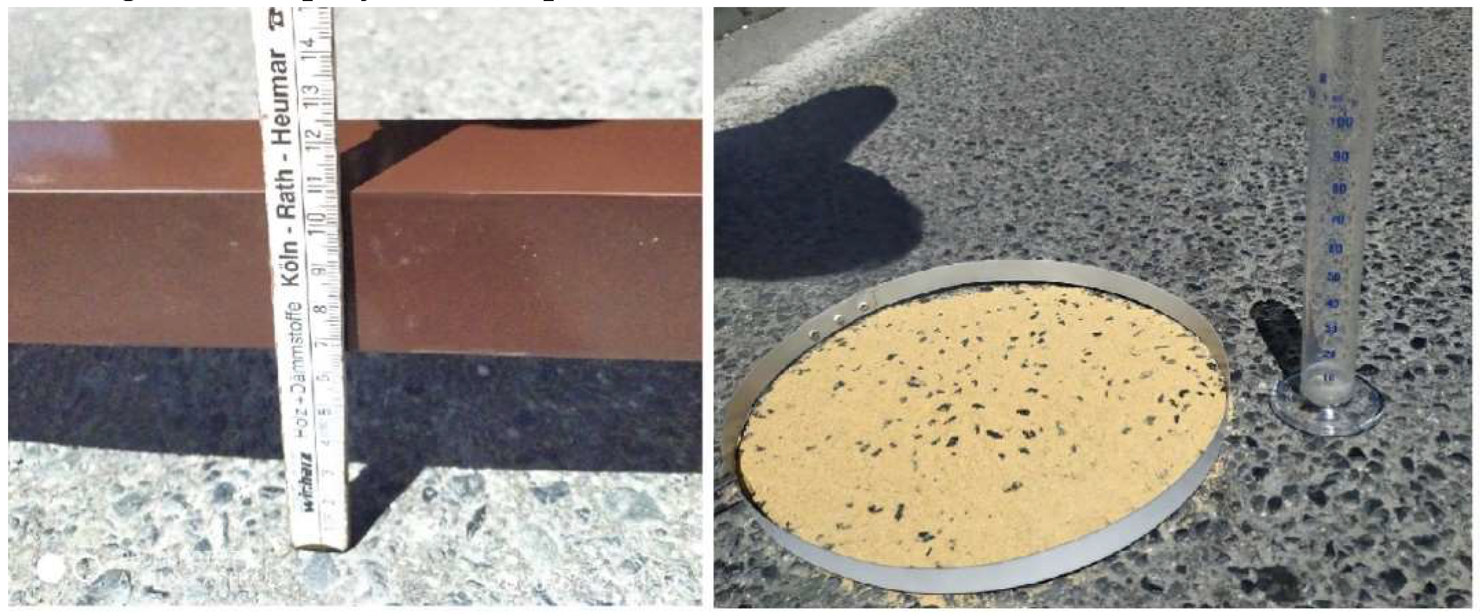
Figure 2.
Linear-SVM vehicle detection and classification.
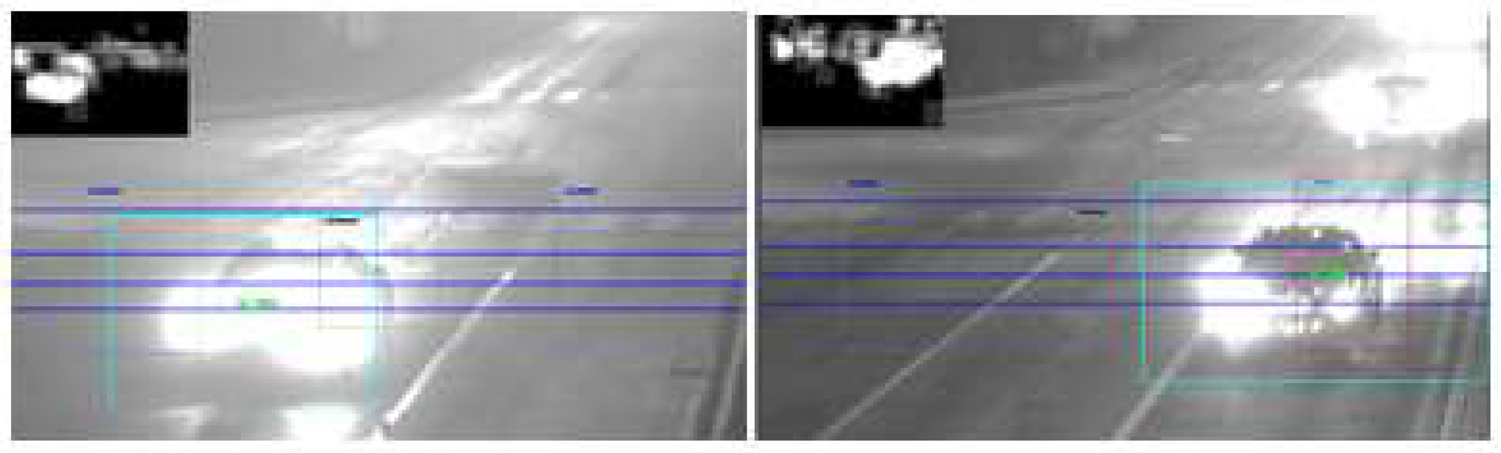
Figure 3.
MLP with one hidden layer.
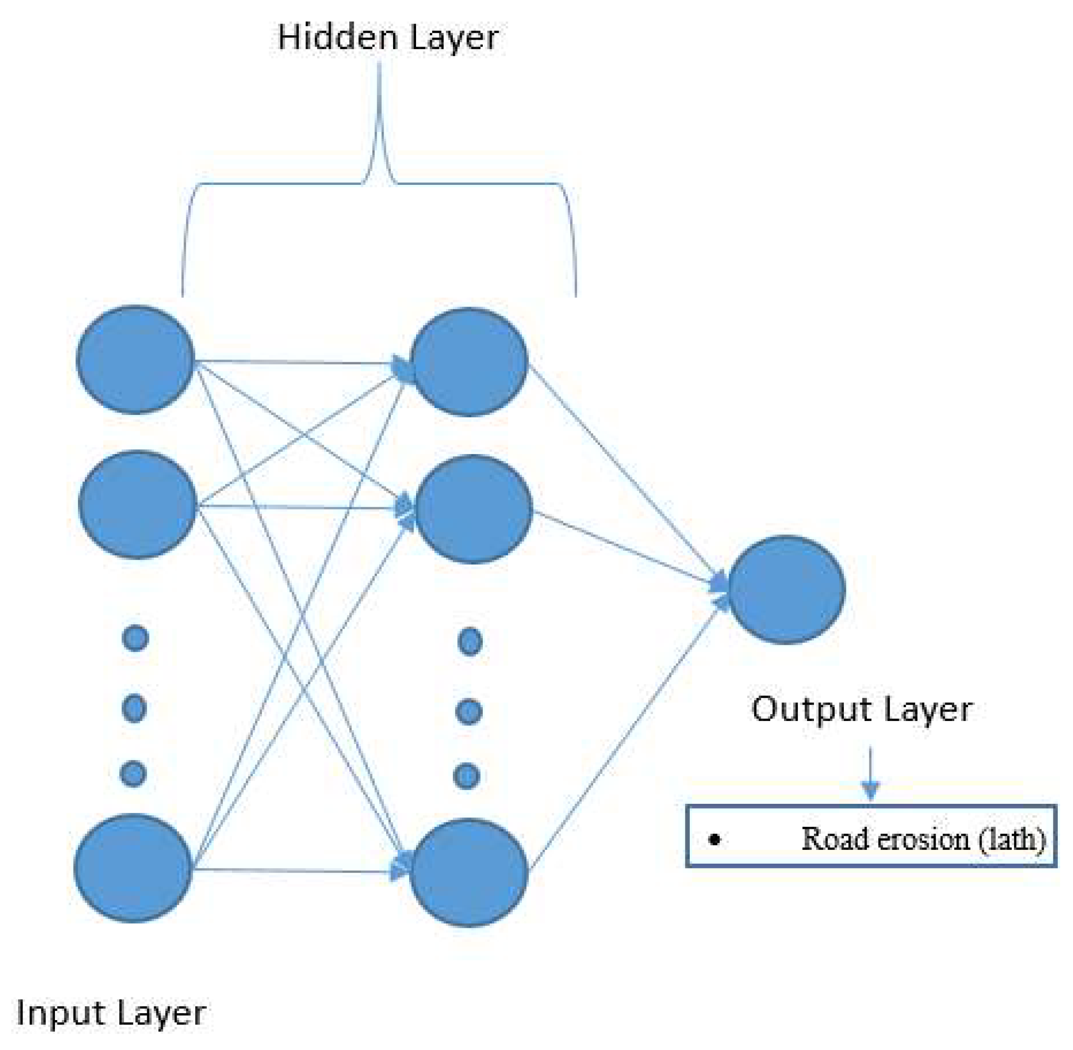
Figure 4.
MLP "lath" predictions vs measured statistical value.
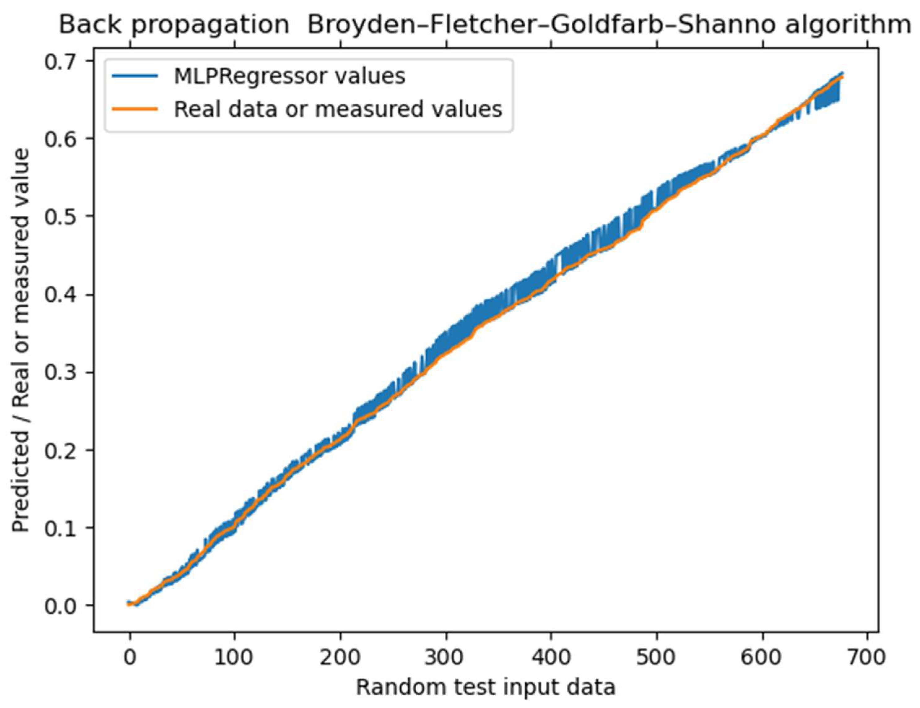
Figure 5.
"Lath" with measurements taken 75m from the intersection.
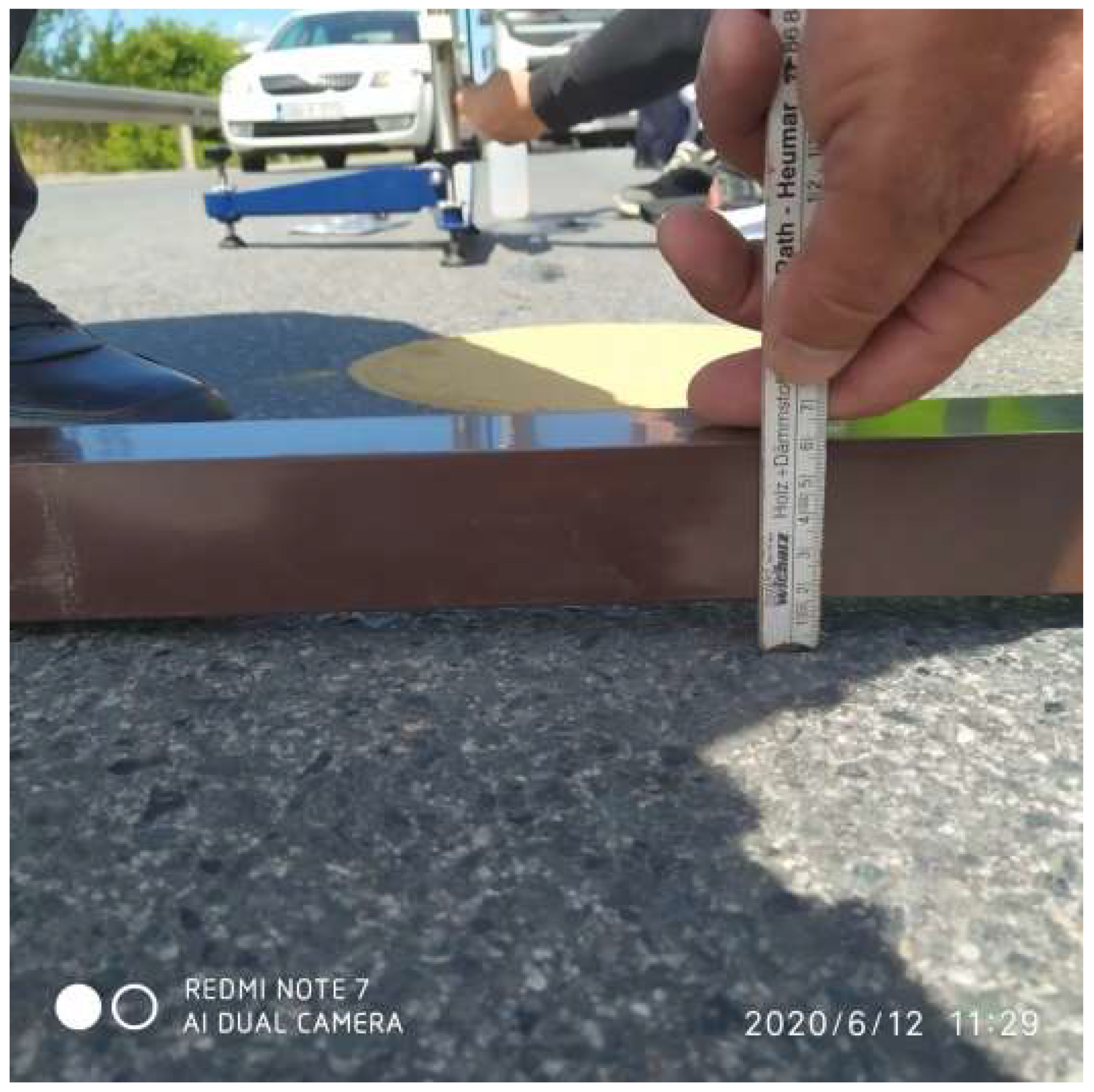
Figure 6.
Intersection two sketch with indicated points of observations as T1 and T2 (meter).
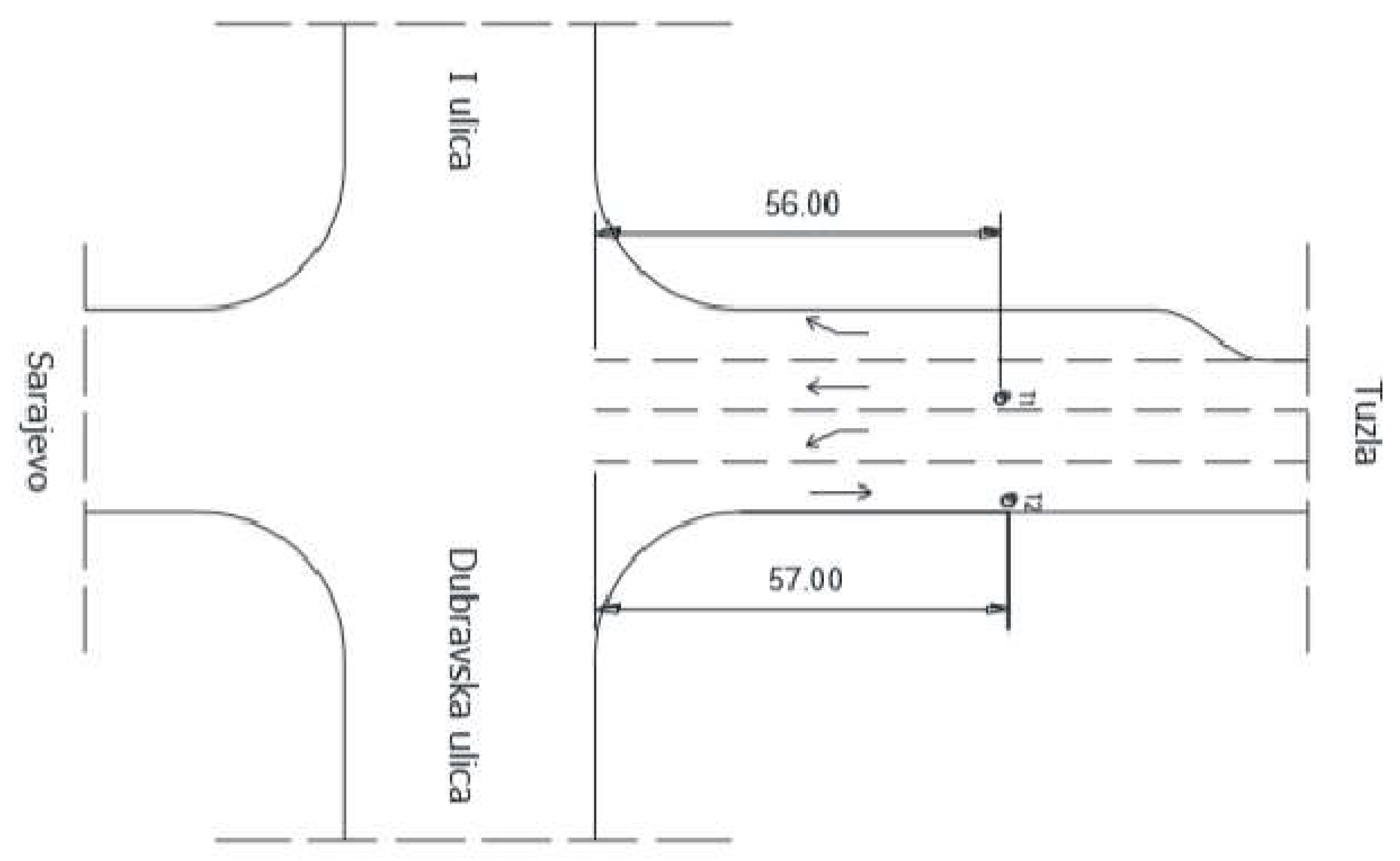
Figure 7.
A visual representation of the intersection used. T1 lane is used to teach AI the erosion and T2 is used for prediction.
Figure 7.
A visual representation of the intersection used. T1 lane is used to teach AI the erosion and T2 is used for prediction.
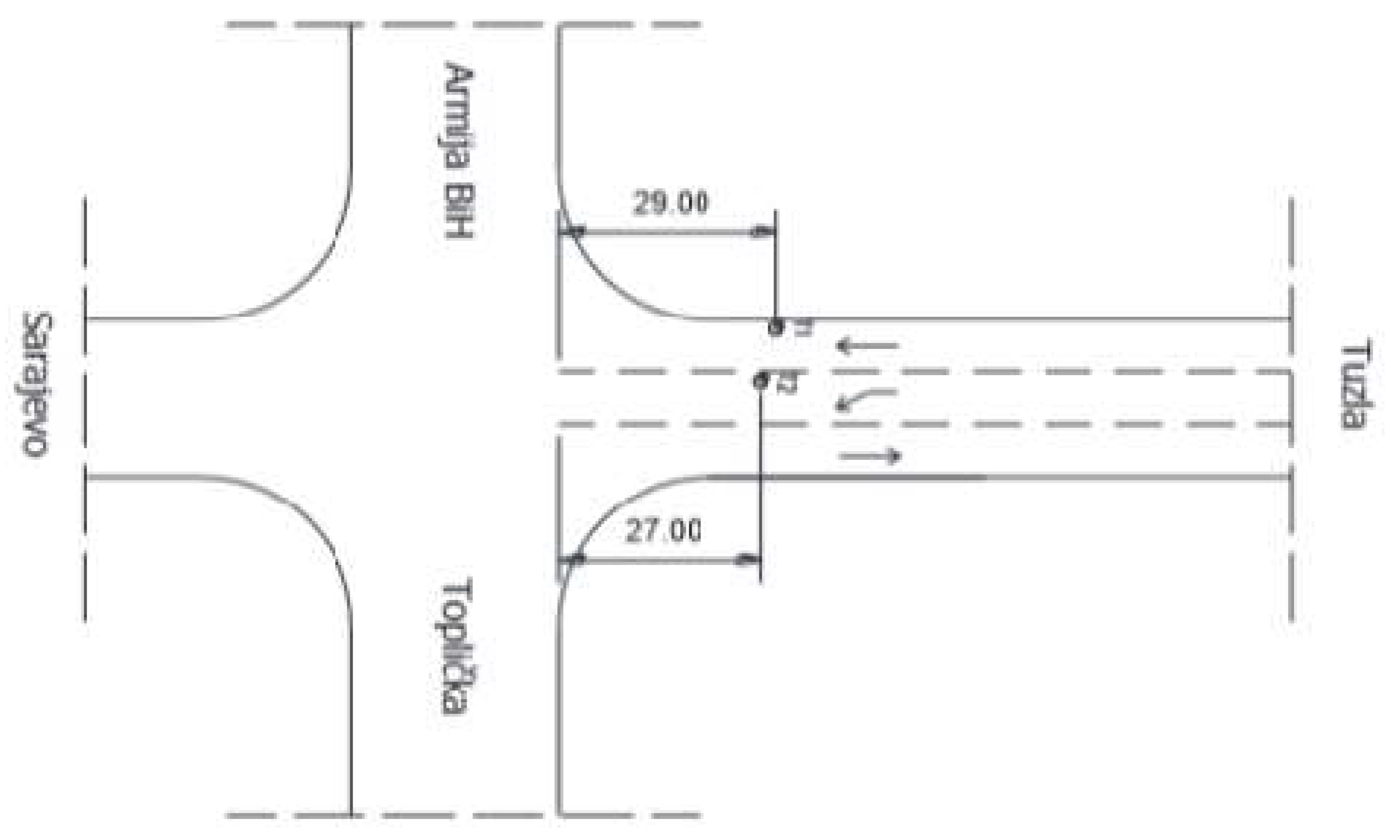
Figure 8.
Model based visualization for the 10-year road erosion (lath).

| Day | # of LW vehicle | # of HW vehicle | Time period (h) | Time on junction (h) HW | Time on junction (h) LW | # of HW going to a complete stop | Road erosion (lath) |
|---|---|---|---|---|---|---|---|
| 1 | 2977 | 225 | 24 | 0.87 | 9.74 | 51 | 0.021 |
| 2 | 6235 | 424 | 48 | 1.64 | 20.40 | 96 | 0.041 |
| 3 | 9423 | 625 | 72 | 2.42 | 30.83 | 142 | 0.062 |
| 4 | 12784 | 839 | 96 | 3.25 | 41.83 | 190 | 0.083 |
| 5 | 16018 | 996 | 120 | 3.86 | 52.41 | 225 | 0.103 |
| 6 | 18627 | 1069 | 144 | 4.15 | 60.95 | 242 | 0.124 |
| 7 | 21828 | 1251 | 168 | 4.85 | 71.42 | 283 | 0.145 |
| 8 | 24944 | 1437 | 192 | 5.57 | 81.62 | 325 | 0.166 |
| # of LW vehicle | # of HW vehicle | Time period (h) | Time on junction (h) HW | Time on junction (h) LW | # of HW going to a full stop | Road erosion (lath) | Predicted value |
|---|---|---|---|---|---|---|---|
| 11551382 | 1144688 | 40584 | 57.51 | 9787.6 | 10064 | 16 | 16 |
| 11551382 | 1144688 | 40584 | 100 | 19000 | 20000 | 30 | 30 |
| # of LW vehicle | # of HW vehicle | Time period (h) | Time on junction (h) HW | Time on junction (h) LW | # of HW going to a full stop | Predicted value |
|---|---|---|---|---|---|---|
| 0 | 0 | 0 | 0 | 0 | 0 | 0.021 |
| 1000000 | 100000 | 10000 | 400 | 100 | 100 | 0.41 |
| 1000000 | 100000 | 10000 | 4000 | 100 | 1000 | 7.18 |
| 1157278 | 156707 | 8544 | 575 | 4057 | 35385 | 13.5 |
| # of LW vehicle | # of HW vehicle | Time period (h) | Time on junction (h) HW | Time on junction (h) LW | # of HW going to a full stop | Road erosion (lath) | Road erosion (sand) | Road erosion (SRT) |
|---|---|---|---|---|---|---|---|---|
| 11551382 | 1144688 | 40584 | 4206 | 5049 | 40000 | 16.62 | 60 | 40 |
Table 5.
Road erosion (lath) value predictions for the left lane.
| YEAR | # of LW vehicle | # of HW vehicle | Time period (h) | Time on junction (h) HW | Time on junction (h) LW | # of HW going to a full stop | Road erosion (lath) |
|---|---|---|---|---|---|---|---|
| 2016 | 1260235 | 59554 | 8760 | 231.0 | 4123.6 | 9410 | 0.19 |
| 2017 | 2466064 | 116648 | 17520 | 452.4 | 8069.1 | 18431 | 4.73 |
| 2018 | 3703982 | 176937 | 26280 | 686.2 | 12119.7 | 27957 | 9.44 |
| 2019 | 4973366 | 242763 | 35040 | 941.5 | 16273.2 | 38357 | 14.25 |
| 2020 | 6244993 | 307140 | 43800 | 1191.1 | 20434.0 | 48529 | 19.10 |
| 2021 | 7544905 | 375202 | 52560 | 1455.1 | 24687.4 | 59282 | 24.10 |
| 2022 | 8873103 | 446951 | 61320 | 1733.3 | 29033.3 | 70619 | 29.63 |
| 2023 | 10229586 | 522386 | 70080 | 2025.9 | 33471.8 | 82538 | 36.66 |
| 2024 | 11614355 | 601507 | 78840 | 2332.7 | 38002.9 | 95039 | 46.68 |
| 2025 | 13027410 | 684314 | 87600 | 2653.8 | 42626.5 | 108122 | 59.98 |
Disclaimer/Publisher’s Note: The statements, opinions and data contained in all publications are solely those of the individual author(s) and contributor(s) and not of MDPI and/or the editor(s). MDPI and/or the editor(s) disclaim responsibility for any injury to people or property resulting from any ideas, methods, instructions or products referred to in the content. |
© 2023 by the authors. Licensee MDPI, Basel, Switzerland. This article is an open access article distributed under the terms and conditions of the Creative Commons Attribution (CC BY) license (http://creativecommons.org/licenses/by/4.0/).
Copyright: This open access article is published under a Creative Commons CC BY 4.0 license, which permit the free download, distribution, and reuse, provided that the author and preprint are cited in any reuse.


