
Submitted:
16 June 2023
Posted:
19 June 2023
You are already at the latest version
Abstract
Friction has long been an important issue in multibody dynamics. Static friction models apply appropriate regularization techniques to convert the stick inequality and the non-smooth stick-slip transition of Coulomb’s approach into a continuous and smooth function of the sliding velocity. However, a regularized friction force is not able to maintain long-term stick. That is why, dynamic friction models were developed in the last decades. The friction force depends herein not only on the sliding velocity but also on internal states. The probably best known representative, the LuGre friction model, is based on a fictitious bristle but realizes a too simple approximation. The recently published second order dynamic friction model describes the dynamics of a fictitious bristle more accurately. Its performance is compared here to stick-slip friction models, developed and launched not long ago by commercial multibody software packages.
Keywords:
Dynamic Friction Model
; Commercial Stick-Slip Friction Models
; Long-term Stick
; Multibody Dynamics
1. Introduction
Friction has long been an important issue in multibody dynamics. Today, static and dynamic friction force models are applied in multibody dynamics [1]. Static friction models usually apply appropriate regularization techniques to convert the stick inequality and the non-smooth stick-slip transition of Coulomb’s approach into a continuous and smooth function of the sliding velocity. However, a regularized friction force is not able to maintain long-term stick. That is why, dynamic friction models were developed in the last decades. The friction force depends herein not only on the sliding velocity but also on internal states. The probably best known representative, the LuGre friction model, is based on a fictitious bristle but realizes a too simple approximation [2]. A second order dynamic friction model describes the dynamics of a fictitious bristle more accurately. It was introduced in [2] as a reference and performed well in standard stick-slip examples as well as in a more practical model of a festoon cable system. In the present paper the second order dynamic friction model is compared to stick-slip friction models, developed and launched not long ago by commercial multbody software packages. They are presented and analyzed in [3]. It turns out that the concepts of ADAMS and Recurdyn are quite similar but different from the Simpack stick-slip model. That is why, just the ADAMS and the Simpack approaches are used here for the comparison with the second order dynamic friction model.
2. Static and Dynamic Friction Models
The idealized friction model of Coulomb simply distinguishes between sticking and sliding, Figure 1a. The friction force depends on the sliding velocity v and is realized by by combining an inequality with a simple relation
The friction force is proportional to the normal force and characterized by the parameters and , which specify the static and the dynamic coefficients of friction.
Coulomb’s dry friction approach, as defined in Equation (1), is practically unusable in general multibody dynamics because of the inequality representing stick. That is why, dry friction is usually approximated by an unambiguous function, Figure 1b. The regularized characteristics introduces the fictitious velocity , which defines the width of the regularization interval and the dynamic velocity , that characterizes at the range of full sliding, where the simple relation applies. The transitions from the value pairs and as well as are usually modeled by sufficiently smooth functions, like polynomials or trigonometric functions.
Static friction models are widely used in multibody dynamics and control theory. They are able to reproduce stick-slip effects in standard and in a more practical application [2]. Even much simpler regularizations, assuming by just one unique friction value, are in good conformity to dynamic measurements [4]. However, static friction models cannot maintain long-term stick. They describes the friction force just as a function of the sliding velocity . Figure 1b defines a commonly used regularized friction characteristics by a set of “static” () and “dynamic” () friction parameters. However, the use of dynamic friction parameters is no essential criteria for a dynamic friction model, as erroneously assumed in [6].
Dynamic friction models are characterized by the use of internal states. The friction force is then defined by a more complex function , where s collects the internal states. Dynamic friction models are able to reproduce stick-slip effects and maintain long-term stick [5].
A software capable formulation of a friction force model takes also the friction model parameters into account. Then, characterizes a static and a dynamic friction model, where p collects the friction model parameters.
The well known LuGre friction model uses the displacement z of a fictitious bristle as an internal state. However, as demonstrated in [2], the LuGre approach represents just a first step approximation to the dynamics of a massless bristle, which results in several drawbacks of this dynamic friction model. If the mass of the fictitious bristle is also taken into account, this results in a second order dynamic friction model, which was introduced in [2] as a reference and performed well in standard stick-slip examples and in a more practical model of a festoon cable system.
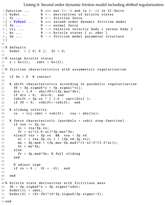
The second order bristle dynamics is defined by
where approximates the inertia force of the fictitious bristle, describes the friction force, models the bristle as a visco-elastic element, and represents the component of the contact point velocity that is perpendicular to the contact normal. Just as with the LuGre model, and describe the stiffness and the damping of the fictitious bristle. The fictitious mass of the bristle is defined by
which represents the aperiodic case of the homogenous second order differential equation (2) thus avoiding unwanted oscillations of the fictitious bristle. The second order dynamic bristle model implies with two internal states. It is provided as a Matlab function in the Appendix by Listing 4.
The stick-slip models of Adams and RecurDyn describe the dynamic friction force just as a function of the contact point velocity and approximate the static friction force by a two-dimensional function , where x is a fictitious displacement [3]. A smooth function of the contact point velocity , which is not explained in detail in the user manual, describes the transition from to . The fictitious displacement serves as an internal state and generates the static friction force or the static friction coefficient as a nonlinear function of x by adding a viscous damping term.
Simpack provides a stick-slip model which realizes, like the Coulomb’s approach in Figure 1a, a sudden drop from the static to the dynamic friction coefficient [3]. In the adhesion region the friction force is approximated by a visco-elastic element whose deflection again represents an internal state of this stick-slip model.
3. Long-term stick of the second order dynamic friction model
By applying an appropriate horizontal shift to the regularized friction characteristics, as indicated in Figure 1c, the second order dynamic friction model can maintain long-term stick. The steady state solution ( and ) of the fictitious bristle dynamics (2) provides the required sticking force as
The second order dynamic friction model describes here the transition from the static to the dynamic friction force by a cubic polynomial and defines the friction force in the regularization range by a parabolic function. Then
delivers the corresponding horizontal shift. The static friction force is defined by and adjusts the horizontal shift to the sign of the required sticking force value.
Figure 2 provides a simple test-bench which is used here to demonstrate the long-term sticking quality of the second order dynamic friction model and in the following for a comparison to the stick-slip models of ADAMS and Simpack.
A body of unit mass is in contact to a horizontal rough plate. It is exposed to a horizontal force , which is continously increased in the interval from to the final value . The friction parameters , and , model a regularized friction characteristics as defined in Figure 1b. The bristle parameters are adjusted to the body and the friction parameters by estimation a reference friction force of and defining a reference bristle deflection of . Then, provides the bristle stiffness. The reference friction force corresponds with a reference mass of which provides the damping of the fictitious bristle as if a viscous damping rate of is assumed hereby.
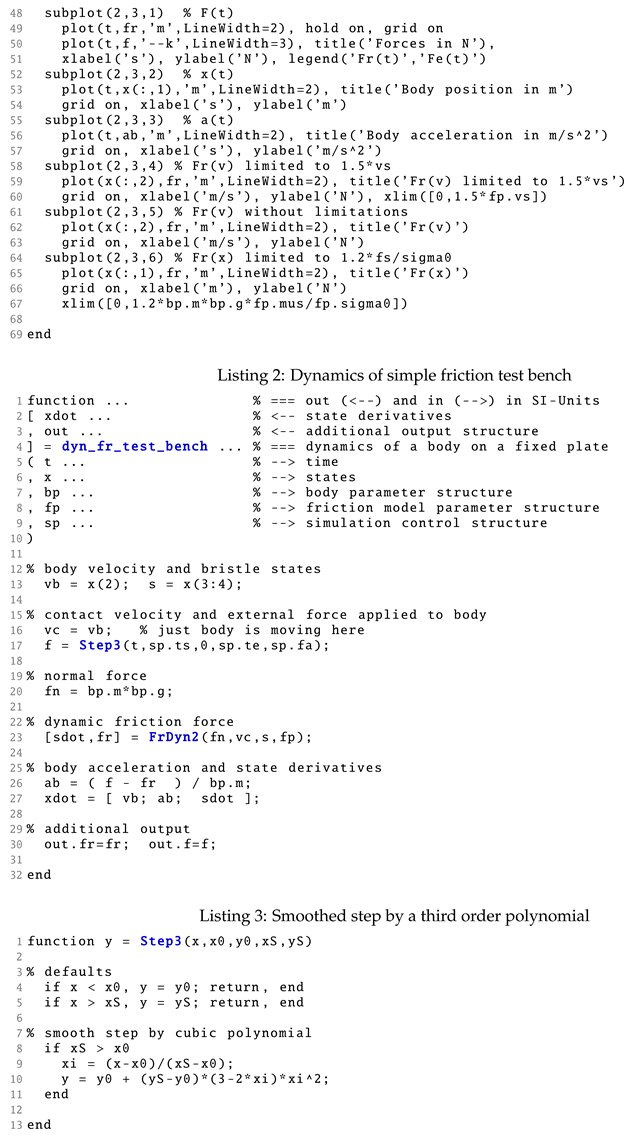
The Matlab script, provided in the Appendix by Listing 1, performs simulations with different step durations. It applies the standard implicit solver ode15s where the default tolerances are changed to RelTol=1.e-6 and AbsTol=1.e-9 because the reference bristle deflection was chosen very small in this example. The Matlab function dyn_fr_test_bench, provided in the Appendix by Listing 2, computes the dynamics of the simple friction test bench including the second order dynamic friction model as a set of first order differential equations. The Matlab functions Step3 and FrDyn2, defined in the Appendix by Listings 3 and 4 provide the step input and the dynamics of the second order friction model. The simulation results, plotted in Figure 3 demonstrate that the second order dynamic friction model perfectly maintains long-term stick.
The excitation force is slowly increased in the time interval from to 99 % of the static friction force , which is given here by . In the subsequent time interval the force is kept constant. The friction force , generated by the second order dynamic friction model counteracts the excitation force , upper left plot in Figure 3. Note that the friction force, as defined by the free body diagram in Figure 3b, points in the opposite direction of the contact point velocity. The tip of the bristle sticks to the ground because the excitation force does not exceed the static friction force. Then, the bristle deflection z coincides with the body displacement u and provides the friction force as a function of the bristle deflection , as demonstrated by the lower right plot in Figure 3. As a consequence, the body shifts slightly and comes to a stand-still at the steady state value of . The friction force diagram in the upper right plot of Figure 3, shows that the second-order dynamic friction model can reproduce the ambiguous part of Coulomb’s friction law at vanishing contact point velocities .
A static friction model describes the friction force just as a function of the sliding velocity, . A typical regularization without any horizontal shift is illustrated in Figure 1. A static friction model can reproduce the required friction force but definitely cannot maintain stick for longer time intervals, Figure 4.
In the regularization range, the friction force characteristics is described by a parabolic function. This pre-defined function, plotted in the right graph of Figure 4 by a thin dashed line, perfectly coincides with the computed friction force plotted by a solid thick line. The parabola delivers the required steady state friction force of at the velocity of . As a consequence, the body does not come to rest but continues to move inexorably at this velocity.
4. Break-away and stick-slip transition
The friction test-bench, defined in Figure 2, consists of a body in contact to a horizontal rough plate. The excitation force is now slowly increased within from to the final value , which exceeds the adhesion limit of by 5 %. The excitation force modeled by a third order polynomial reaches the adhesion limit at time .
The simulation results are plotted in Figure 5. The dashed blue line, the solid black line, and the dotted red line represent the results computed with the second order dynamic friction model (FrDyn2), the ADAMS stick-slip model, and the Simpack stick-slip model.
At first (), the body remains in a quasi-static equilibrium, where the slowly increasing excitation force is perfectly counteracted by a friction force generated by each of the friction models, as demonstrated in Figure 5a where the lines for and perfectly coincide in the time interval . In general, the friction models under consideration generate friction forces depending not only on the contact velocity but also on internal states. The FrDyn2 model uses the displacement z of a fictitious bristle and its time derivative as internal states . In the quasi-static equilibrium mode the velocity of the body and the time derivative of the bristle deflection are negligible small and . In this mode the tip of the fictitious bristle sticks to the ground, which results in a bristle deflection that equals the body displacement . The compliance of the fictitious bristle is modeled by a viscous force element, . In the quasi-static equilibrium mode the body acceleration is negligible small too, as indicated in Figure 5b by the time history in the time interval . According to Equation (2) the friction force generated by the FrDyn2 model corresponds then to the elastic part of the bristle force, . The quasi-static force equals the static friction force at the reference displacement of
The adhesion range is characterized by a vanishing sliding velocity () and extends here to displacements in the range of . In this range the friction force is generated as a function of the displacement, where the FrDyn2 model and the stick-slip model of Simpack apply a linear and the stick-slip model of ADAMS a nonlinear digressive function, Figure 5f. The ADAMS manual does not specify the type of nonlinearity but as indicated by the solid black line in Figure 5f it approaches the limit value at the reference displacement defined in (6) with a vanishing inclination.
The stick-slip model of Simpack is based on Coulomb’s approach, where the friction force drops in an instant from the static to the dynamic value as soon as the excitation force exceeds the static friction force at , Figure 5a and Figure 5d in particular. The transition from the static to the dynamic friction force are modeled in the FrDyn2 and the ADAMS stick-slip model as functions of the velocity v controlled by the parameters and . The FrDyn2 model applies a cubic polynomial which is shifted in the horizontal direction to maintain stick at , as indicated in Figure 1. As can be seen by inspecting Figure 5e, the FrDyn2 model generates a friction force characteristics (dashed blue line) which reproduces the pre-defined and horizontally shifted one (magenta colored circles) nearly perfectly. The friction characteristics produced by the ADAMS stick-slip model is quite similar (solid black line). Most likely, ADAMS models the transition by a 5th order polynomial. As a consequence, the FrDyn2 and the ADAMS stick-slip models produce slightly and slightly more delayed drops in the time histories of the computed friction forces, Figure 5d.
Figure 5b and Figure 5c illustrate the break-away effect at by the time histories of the body acceleration and the body displacement . All friction models under consideration approximate sliding at by a constant friction force . Viscous components in the friction force are not considered here. The free body diagram in Figure 2b delivers the linear momentum
for the body of mass . At which includes the applied force is defined by and the friction force is represented by its dynamic value . Then, the maximum acceleration of the body is defined by
which is exactly reproduced by the friction models, Figure 5b.
5. Dynamic Response
A pulse load excitation, performed in [2], revealed the tendency of dynamic friction models to produce dynamic overshoots in the friction force time histories. That is why, the test-bench defined in Figure 2 is now exposed to excitation forces where the amplitude is 5 % less than the static friction force and the step duration is varied from to . The corresponding simulation results are shown in Figure 6. The solid thin grey line represents the excitation force , the dashed blue line, the solid black line, and the dotted red line mark the friction forces computed with the FrDyn2, the ADAMS stick-slip, and the Simpack stick-slip models.
The time histories of the friction forces perfectly coincide with the excitation force at a step duration of , Figure 6a. All friction models operate here in a quasi-static sticking mode where the friction forces are practically generated as a function of the body displacement, as already illustrated in Figure 5e and in this specific case by Figure 7.
The forces generated by the friction models depend here practically not on the velocity but only on the displacement of the body u, Figure 7a and Figure 7b. In case of the FrDyn2 and the Simpack stick-slip models holds, which provides the friction force at the steady state displacement , as indicated in Figure 7b and Figure 7c by thin dashed black lines. ADAMS models the friction force a quasi-static sticking mode by a strongly nonlinear and degressive function of the displacement. The ADAMS manual does not specify this function but the simulation results provide the friction force at the steady state displacement , Figure 7b and Figure 7c. As expected from the time histories plotted in Figure 6a, the time histories of the body displacement reach their steady state values and at without any overshoots, Figure 7c.
In a quasi-static mode the tip of the fictitious bristle, which forms the basis of the FrDyn2 model, sticks to the ground. Then, the linear momentum (7) of the body in the simple friction test bench simplifies to
where the quasi-static friction force is generated by the bristle compliance and holds in addition. The simplified equation of motion (9) is characterized by the eigen-frequency and delivers the value and its of corresponding oscillation period as
As a consequence, even a rather short step duration of will still represent a subcritical excitation of the simple friction test bench. The time histories of the friction forces exhibit just a tiny overshoot at , Figure 6b.
The situation becomes complicated for step durations , Figure 6c and Figure 6d. The Simpack stick-slip model (dotted red line) generates now significant overshoots, which amount to
The values exceed the steady state value by % and % and even the static friction value by % and %, which calls into question the physical basis of this stick-slip model. The time histories of the friction forces generated by the FrDyn2 and the ADAMS stick-slip models (dashed blue and solid black lines) differ somehow. But both models limit the friction force to the static value , as expected from friction models, in general.
The friction models generate now friction forces which strongly depend on the body velocity and the body displacement u, Figure 8a and Figure 8b.
The Simpack stick-slip model (dotted red line) generates a time history of the body displacement which approaches the quasi steady state value with a small overshoot shortly after the step duration of , Figure 8c. The FrDyn2 model overshoots and partly slides resulting in displacements at which exceed with the quasi steady state value of significantly. Hence, the FrDyn2 model generates a dynamic break-away effect at high frequent excitation loads, which are close (here 95 %) to the static friction force. The time history of the body displacement shows a strange behavior for the ADAMS stick-slip model, solid black line in Figure 8c. At first (), it approaches the quasi steady state value of the FrDyn2 and Simpack solution and then () it starts to decrease very slowly but the simulated time interval is too short to indicate a limit value.
A simulation with the ADAMS stick-slip model over a longer time period results in the time history of the body displacement as plotted in Figure 9,
where the section shown in Figure 8c has a light grey background. It seems that ADAMS applies in its stick-slip model different time constants for the increase and decrease of the body displacement . The force excitation with a step duration of is much faster than the dynamics of the friction test bench. The body displacement reaches its maximum value at which corresponds to oscillation period computed in (10). The decay from the maximum displacement to the steady state value takes about , which is fourteen times as much. This strange behavior was also reported in [3] where pulse loads are applied to a single mass resting on a horizontal plate. At the end of a series of impulse loads each of magnitude , the body returned to its initial position. However, in the present example a small but permanent deviation of remains, Figure 9. This indicates that the ADAMS stick-slip model also tends to slip partly, when high frequent excitation loads close to the static friction force are applied.
6. The festoon cable system model
A planar model of a festoon cable system is used in [2] to asses different friction models in a more practical example. The model consists of three cable and two trolley masses, Figure 10.
At the beginning the towing trolley is fixed at . The equilibrium position of the cable system places the trolleys at , , and locates the cable masses at , , , as well as . The non-holonomic constraint relates the movements of the towing trolley to a pre-defined velocity profile . The velocity profile, defined by the solid grey lines in Figure 11a, models an extension maneuver, which moves the towing trolley from the initial position to a final position of .
The Matlab simulation with the second order dynamic friction model (FrDyn2) generates the output at every simulation step. It applies the ode15s solver with error tolerances of RelTol=1.e-6 and AbsTol=1.e-9. The ADAMS and Simpack simulations were performed with an output step size of . The dashed blue, the solid black, and the dotted red lines mark the results obtained by the FrDyn2, the ADAMS, and the Simpack stick-slip models.
The movement of the towing trolley ends at . After that the trolleys perform to and fro motions which at are indicated by sign changes in the time histories of trolley velocities and . An arrow pointing from over down to highlights such an event, in particular. The dynamic motions of the cable masses induce variations in the normal forces and acting between the trolleys and the rail, Figure 11b. The time histories of the velocities , and the normal forces , generated with FrDyn2 and the stick-slip models of ADAMS and Simpack match nearly perfectly. However, the time histories of the friction forces , exhibit some discrepancies, Figure 11c. In particular when the trolley velocities change their signs or during a sticking period of trolley 2.
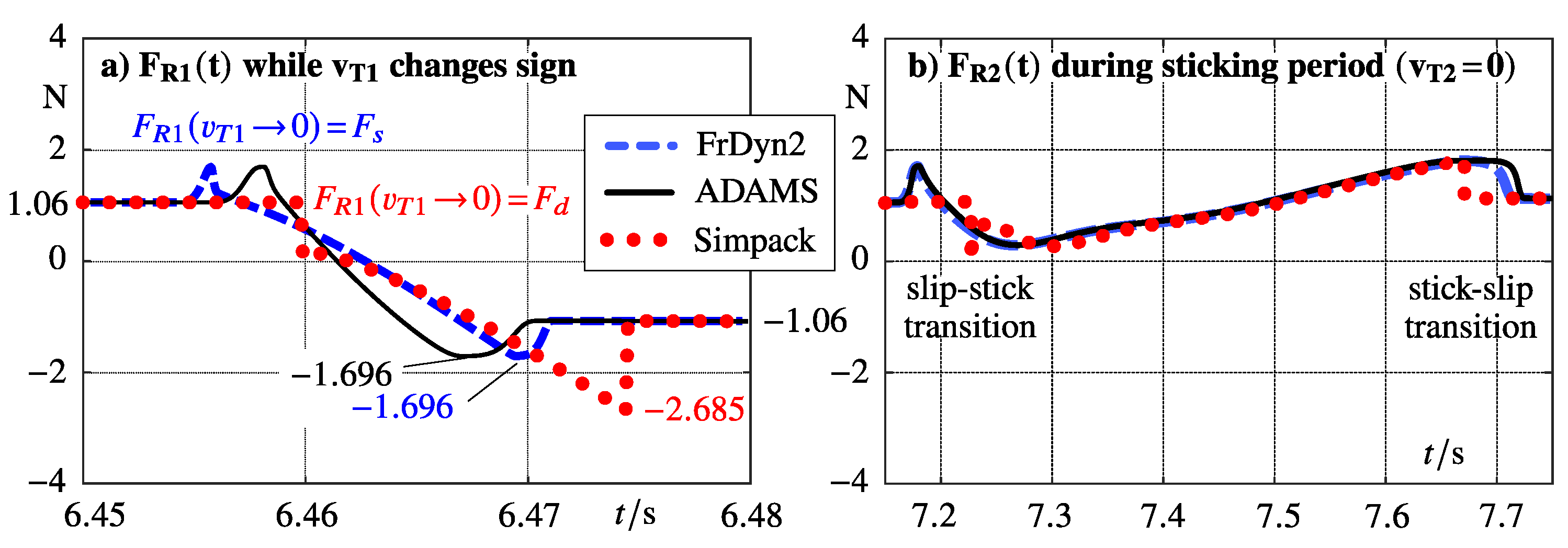
The plots in Figure 12 focus on a sign change of the trolley velocity at and a sticking period of trolley 2 in the time interval .
In the very short time interval the normal force between trolley 1 and the rail amounts to as indicated in Figure 11b. The friction values defined in Figure 10 provide in this case a static friction force of and a dynamic friction force of . At times and the first trolley is in a full sliding mode, indicated in Figure 12a by the friction forces and . These sliding modes are perfectly reproduced by the friction models under consideration. Shortly before the sign change in the trolley velocity the friction forces computed by the FrDyn2 and the ADAMS stick slip model make use of the Stribeck effect, which models a velocity dependent transition from the static to the dynamic friction force and vice versa. The Simpack stick-slip model approaches with the dynamic force value and does not reproduce a potential velocity dependent increase of the friction force. The FrDyn2 and the Simpack stick-slip models describe the friction force at by a linear spring, whereas the ADAMS stick slip model uses a nonlinear approach. That is why, the FrDyn2 model (dashed blue line) corresponds in the time interval more to the Simpack (dotted red line) than to the ADAMS stick-slip model (solid black line). The friction forces of the FrDyn2 and the ADAMS stick-slip models are limited to the static value , which results in at . However, The Simpack stick-slip model overshoots and produces the peak-value of which exceeds by nearly 60 % the static friction force or , respectively.
The sticking period is represented quite similar by the friction models under consideration, Figure 12b. Again, the FrDyn2 and the ADAMS stick slip models increase the friction forces from the dynamic to the static value when approaching stand-still at . However, the small time delay of the peak values visible in Figure 12a is not noticeable because of the large time interval applied in this plot. The Simpack stick-slip model is based on the Coulomb’s approach which results in the discontinuities at the slip-stick and stick-slip transitions in the dotted red line.
7. Discussion
The present manuscript compares a second order dynamic friction model (FrDyn2) with the commercial stick-slip models of ADAMS and Simpack. The FrDyn2 model was introduced in [2] as a reference and tested versus the LuGre and a simple regularized friction model. The stick-slip models of ADAMS and Simpack as well as RecurDyn are described and investigated in [3].
The comparison is performed here with a simple friction test bench and a more practical model of a festoon cable system. All models can maintain long-term stick. The FrDyn2 model corresponds partly to the ADAMS and partly to the Simpack stick slip models. The FrDyn2 and the ADAMS stick-slip models show dynamic break-away effects at high frequent excitation loads, which are close (here 95 %) to the static friction force. The Simpack stick-slip model avoids dynamic break-away effects by overshoots in the friction force that far exceed the static friction force. ADAMS models the decay of a friction force overshoot much slower than the increase, whereas the FrDyn2 model considers in both cases the dynamics of the fictitious bristle.
The FrDyn2 model is based on a fictitious bristle characterized by its mass, stiffness and damping. The fictitious mass of the bristle is automatically adjusted to the stiffness and damping parameters. The pre-defined friction force characteristics is described here by piecewise defined polynomials but not limited to this. The bristle parameters can easily be derived from estimated reference friction forces and estimated bristle deflections. The results obtained by the FrDyn2 model are reliable and based on the physical nature of the friction model approach, which makes the second order dynamic friction model to a suitable alternative to commercial stick-slip models.
Author Contributions
Both authors validated the results, wrote, and reviewed the manuscript. Georg Rill developed the second order dynamic friction model, performed the Matlab Simulations, and produced the figures. Matthias Schuderer performed the simulations with the ADAMS and the Simpack stick-slip models. Both authors have read and agreed to the published version of the manuscript.
Data Availability Statement
The Appendix A provides a Matlab script and functions which realize the simple friction test bench including the second order dynamic friction model.
Conflicts of Interest
The authors declare no conflict of interest.
Appeindix A. Simple friction test bench realized in Matlab

References
- Marques, F.; Paulo Flores, P.; Pimenta Claro, J. C.; Lankarani, H. M. A survey and comparison of several friction force models for dynamic analysis of multibody mechanical systems. Nonlinear Dyn2016(86) pp. 1407–1443. Available online: https://link.springer.com/article/10.1007/s11071-016-2999-3 (accessed on 10 June 2023).
- Rill, G.; Schaeffer, T.; Schuderer, M. LuGre or not LuGre.Multibody Syst Dyn 2023. [CrossRef]
- Schuderer, M.; Rill, G.; Schaeffer, Th.; Schulz, C. Friction Modeling from a Practical Point of View. In Proceedings of the ECCOMAS Thematic Conference on Multibody Dynamics July 24–28 2023 Lisbon, Portugal.
- Pires, I.; Ayala, H.; Weber, H. Ensemble Models for Identification of Nonlinear Systems with Stick-Slip. ENOC 2020+2, Lyon, France 2022. Available online: https://enoc2020.sciencesconf.org/386539/document (accessed on 10 June 2023).
- Jing, Q.; Mi, N. Investigation of Selection Mechanism of Friction Models in Multibody Systems. In Proceedings of 5th International Conference on Vehicle, Mechanical and Electrical Engineering (ICVMEE) 2019 pp. 251–260. Available online: https://www.scitepress.org/Papers/2019/88736/88736.pdf (accessed on 10 June 2023).
- Chaturvedi, E.; Mukherjee, J.; Sandu, C. A novel dynamic dry friction model for applications in mechanical dynamical systems. In Proceedings of the Institution of Mechanical Engineers, Part K: Journal of Multibody Dynamics 2023.
Figure 1.
Dry friction: a) Coulomb’s approach, b) regularized approximation, c) shifted regularization.
Figure 1.
Dry friction: a) Coulomb’s approach, b) regularized approximation, c) shifted regularization.
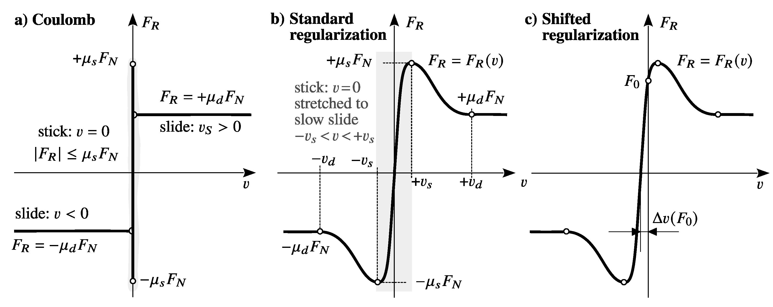
Figure 2.
Simple friction test-bench.
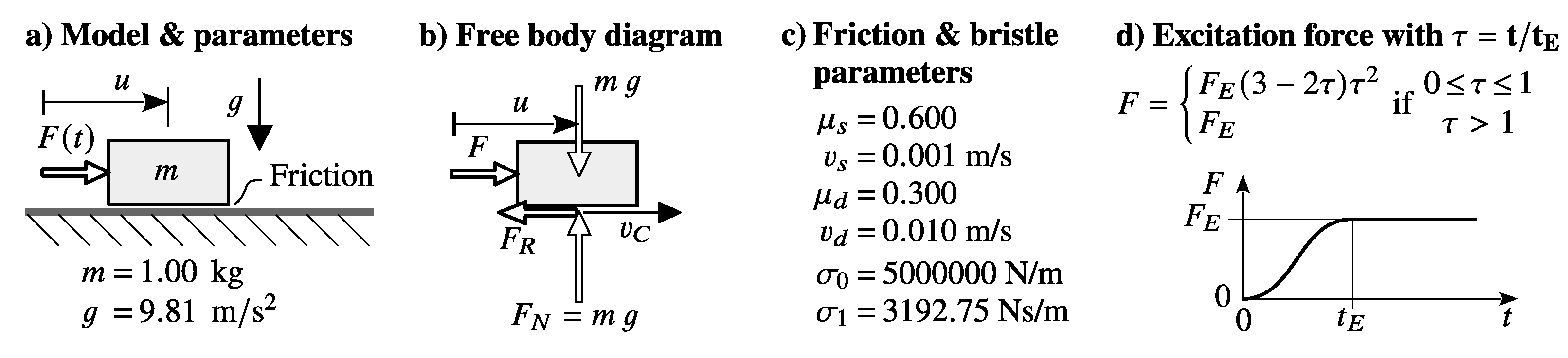
Figure 3.
Long-term stick potential of second order dynamic friction model.
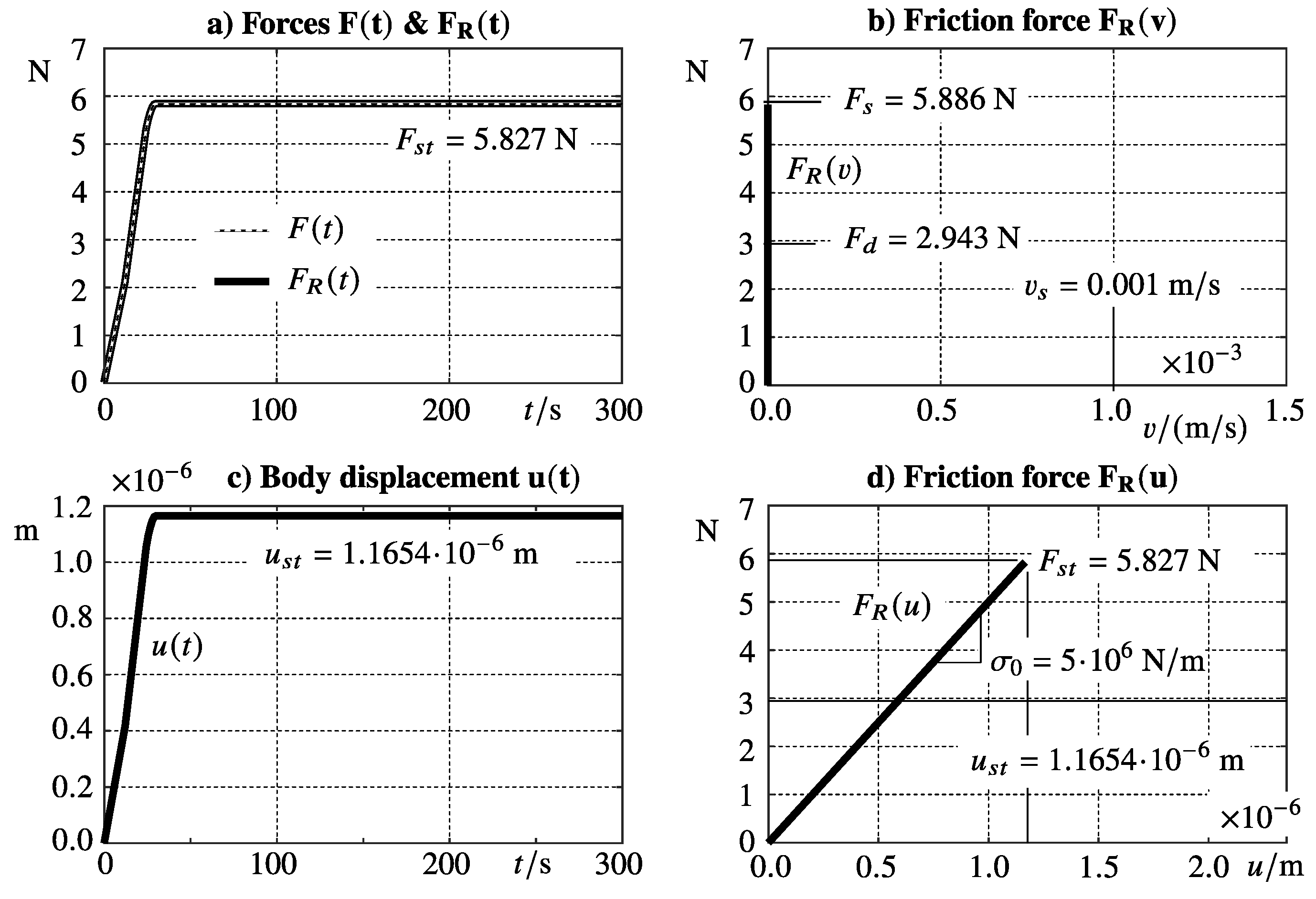
Figure 4.
Slow sliding approximates sticking at a standard static friction model.
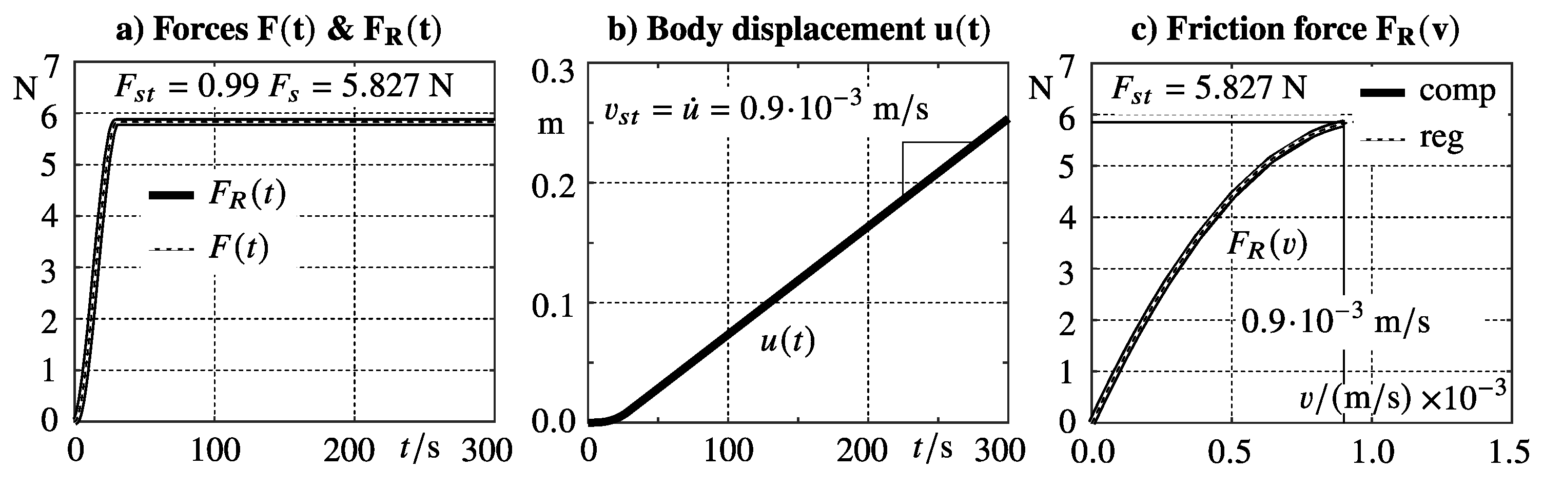
Figure 5.
Friction test-bench simulation results with a force that exceeds the adhesion limit.
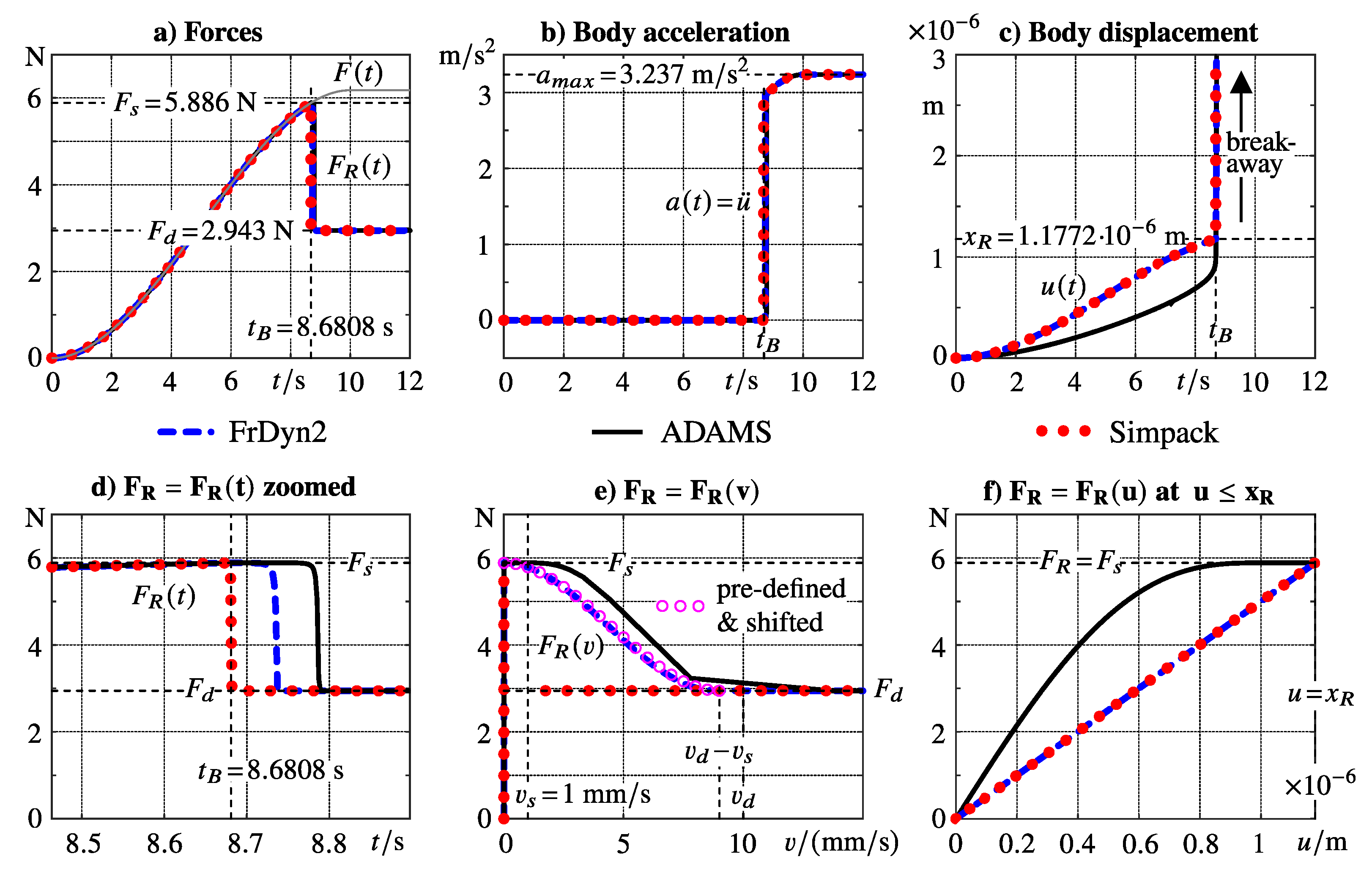
Figure 6.
Dynamic friction forces resulting from step force excitation with different durations.
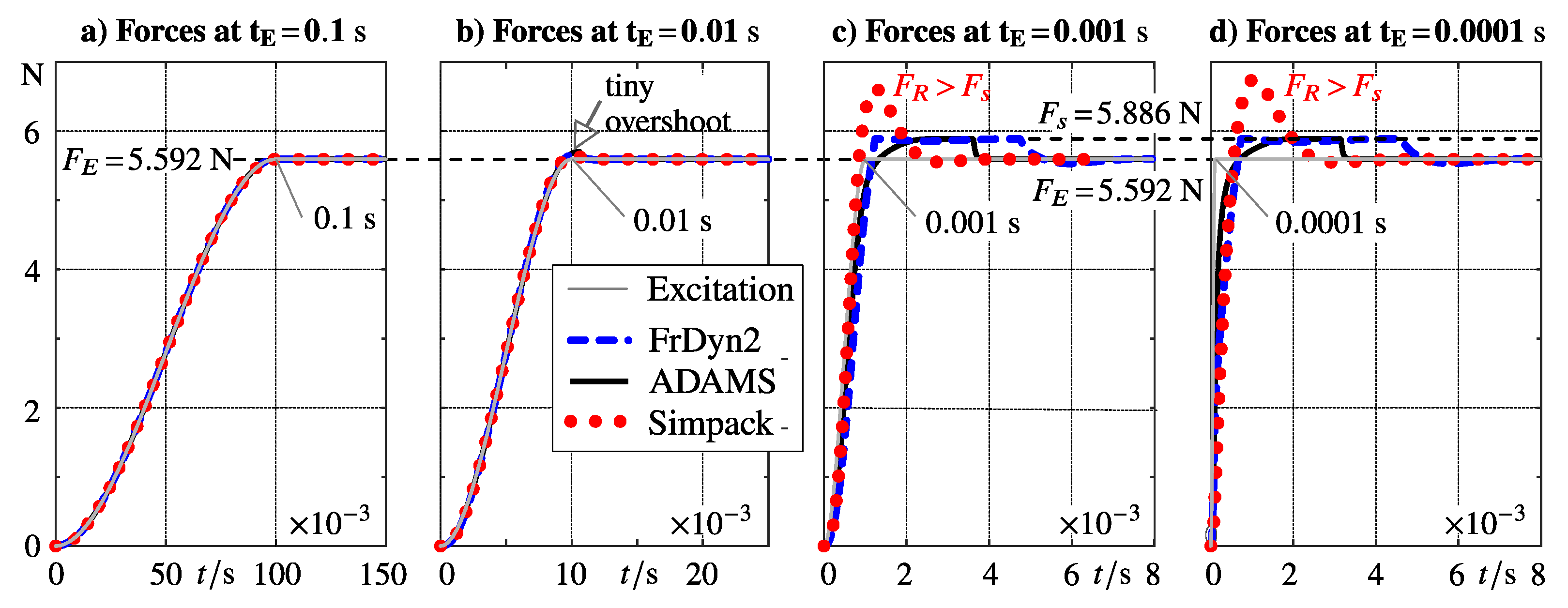
Figure 7.
Friction force characteristics and body displacements at a step duration of .
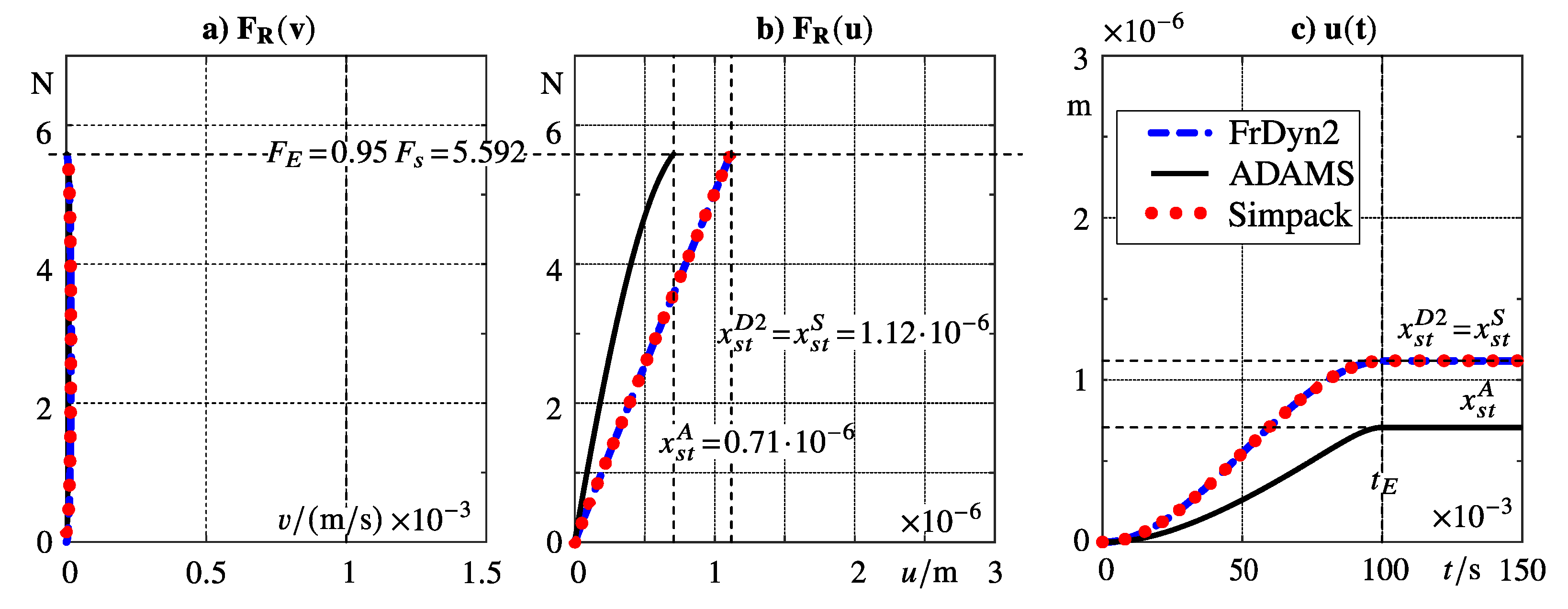
Figure 8.
Friction force characteristics and body displacements at a step duration of .
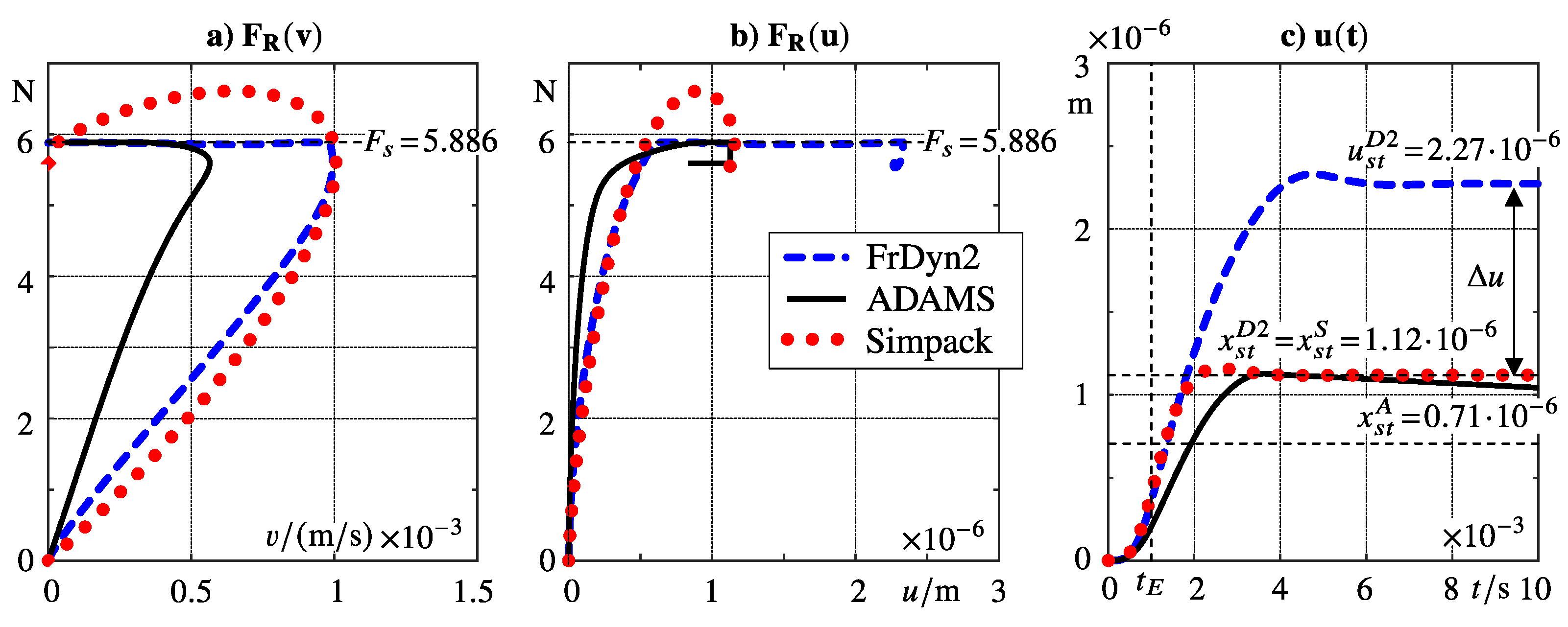
Figure 9.
Body displacements generated with ADAMS at a step duration of .
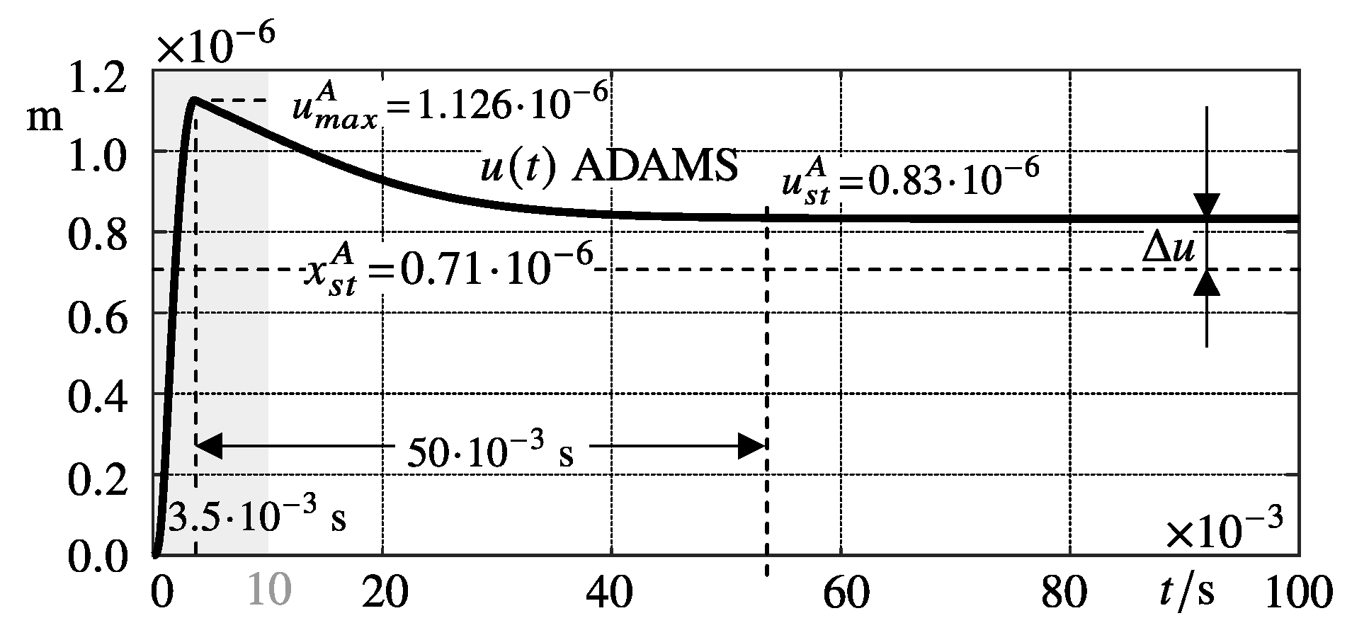
Figure 10.
Multibody model of a crane festoon system as defined in [2].
Figure 10.
Multibody model of a crane festoon system as defined in [2].
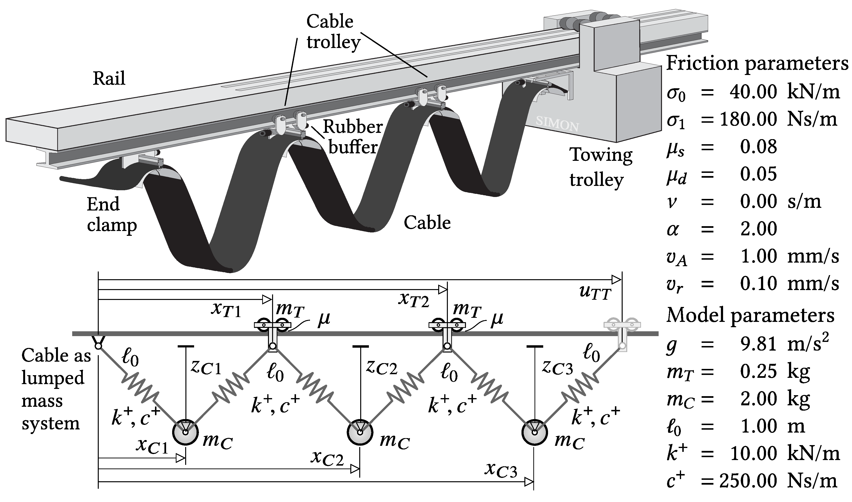
Figure 11.
Results of a simulated festoon extension maneuver.
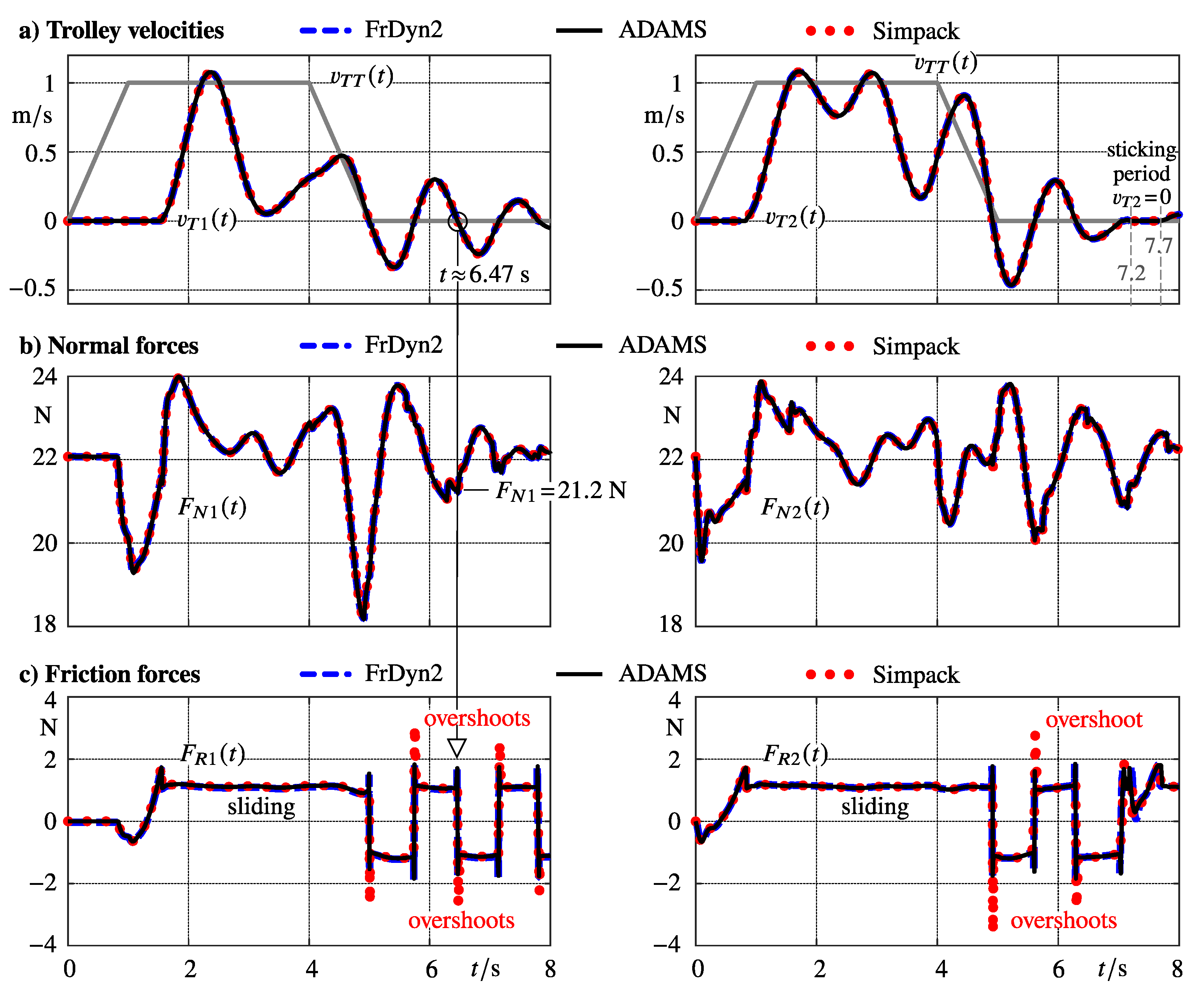
Figure 12.
Friction forces in specific time intervals.
Disclaimer/Publisher’s Note: The statements, opinions and data contained in all publications are solely those of the individual author(s) and contributor(s) and not of MDPI and/or the editor(s). MDPI and/or the editor(s) disclaim responsibility for any injury to people or property resulting from any ideas, methods, instructions or products referred to in the content. |
© 2023 by the authors. Licensee MDPI, Basel, Switzerland. This article is an open access article distributed under the terms and conditions of the Creative Commons Attribution (CC BY) license (http://creativecommons.org/licenses/by/4.0/).
Copyright: This open access article is published under a Creative Commons CC BY 4.0 license, which permit the free download, distribution, and reuse, provided that the author and preprint are cited in any reuse.


