

Submitted:
16 June 2023
Posted:
16 June 2023
You are already at the latest version
Abstract
We propose a method of cooling nuclear spin systems of solid-state nanostructures by application of a time-dependent magnetic field synchronized with spin fluctuations. Optical spin noise spectroscopy is considered as the method of fluctuation control. Depending on the mutual orientation of the oscillating magnetic field and the probe light beam, cooling might be either provided by dynamic spin polarization in an external static field or result from population transfer between spin levels without build-up of a net magnetic moment (“true cooling”).
Keywords:
nuclear spin
; spin noise
; nanostructure
; dynamic polarization
; spin temperature
1. Introduction
The energy transfer between nuclear spins and phonons in solids is known to be extremely slow, especially if the crystal lattice is kept at a cryogenic temperature, so that the spin-lattice relaxation time can reach hours [1,2]. At the same time, energy exchange between nuclear spins due to their magneto-dipole interaction occurs on the spin-spin relaxation timescale of approximately 0.1 millisecond. Off-diagonal elements of the density matrix of the nuclear spin system (NSS) decay within approximately the same time. As a result, the NSS reaches internal equilibrium characterized by a spin temperature that can be many orders of magnitude lower than the lattice temperature, deep into the micro- or even nanoKelvin range [2]. Over the years that passed since the first experimental demonstration of the nuclear spin temperature [3], several methods were developed for cooling the NSS down to ultra-cryogenic temperatures.
Application of an oscillating magnetic field to the nuclear spin system (NSS) is known to warm it up. If an external static magnetic field is applied, this effect amounts to depolarization of nuclear spins and peaks up at NMR frequencies [1]; in zero external field, it manifests itself as a decrease of magnetic susceptibility of the NSS [4]. The question arises whether it is possible to create conditions under which an oscillating field would act in the opposite way, cooling the NSS?
From general considerations, this might be possible if the oscillating field is synchronized with nuclear spin fluctuations. The rate of changing the NSS energy under influence of the field equals
where is the total magnetic moment of the NSS. To provide a net change of the NSS energy, must be correlated with the field; in particular, if an oscillating magnetic field is applied, the averaged over the period time derivative of the energy reads
It is easy to show that in macroscopic solids, where spin fluctuations are negligible, the field-induced change of energy always results in heating up the NSS. Indeed, the mean magnetic moment induced by the field equals . Now, as follows from Eq.(2),
where is the nuclear spin temperature. Here we used the well-known result of the fluctuation-dissipation theorem in the high-temperature limit [5]: . One can see from Eq.(3) that the oscillating field pumps energy into the NSS in case of positive and out of it in case of negative . In both cases, the absolute value of increases, i.e. the interaction of the oscillating magnetic field with the average magnetic moment induced by this field always warms up the NSS.
However, if we are dealing with a finite-size NSS of a nanostructure, its magnetic moment includes a nonzero fluctuating part : . Let us suppose that we can measure in real time. This can be done, for instance, by optical spin noise spectroscopy [6]. Then we can apply an oscillating field in such a way that it would correlate with the nuclear spin fluctuation so that the average product of time derivative of and the magnetic moment would be nonzero:
The resulted energy influx to the NSS would not depend on the NSS spin temperature, as distinct from the warm-up process, and would be linear in the magnetic field (and, consequently, its sign could be made positive or negative at will of the experimentalist). This opens up a possibility of cooling the NSS to low positive or negative temperatures.
In the following, two examples of experimental arrangement in which nuclear spins can be cooled by oscillating magnetic fields are considered. In the first example, application of a constant magnetic field is necessary; here cooling of the NSS is provided by the build-up of nuclear spin polarization parallel or antiparallel to this field. In the second example, the NSS cooling amounts to population change of energy levels of nuclear spins split by Zeeman, spin-spin or quadrupole interactions, and is not necessarily accompanied by net spin polarization (“true cooling”).
2. Dynamic spin polarization by oscillating magnetic field in a static external field
We consider the experimental geometry shown in Figure 1
A constant magnetic field is applied along the axis X. The Z component of the total magnetic moment of the probed volume, , is measured, and the time-dependent magnetic field
is applied along Y. Here is an adjustable transformation factor. One should note, that Eq.(1) is an idealization: in fact, the time-dependent field will inevitably contain an uncontrollable random contribution due to e.g. conversion of the photonic shot noise in the optical channel. The detrimental effect of this noise field will be considered later in Section 4.
Qualitatively, the effect of the time-dependent field on the nuclear magnetic moment is explained by the scheme shown in Figure 2. As is correlated with , the latter is turned always in the same direction, feeding the X-component of magnetization. At the same time, is turned so that it tends to compensate , reducing the amplitude of the transverse spin fluctuation. The latter is on average restored within the transverse relaxation time . On the other hand, since the longitudinal relaxation time is much longer than , accumulates and becomes much greater than the average fluctuation.
The quantitative description of this process is provided by dynamic equations for the components of the magnetic moment :
where is the nuclear gyromagnetic ratio.
In the following, we will develop these equations in the rotating-frame representation. It is the standard technique for the NMR theory, but as we are dealing with fluctuating magnetic moments, we choose to present a detailed derivation of the rotating-frame counterpart of Eqs.(6). In terms of the magnetic moment components in the coordinate frame rotating with the Larmor frequency , and ,
Substituting these expressions into Eq.(6) we obtain
Multiplying the 2nd equation in Eq.(8) by and the 3rd one by and adding up these two equations, we obtain the equation for the time derivative of :
Similarly, by multiplying the 2nd equation in Eq.(8) by and the 3rd one by and subtracting, we obtain the equation for the time derivative of :
The 1st equation in Eqs.(8), Eq.(9) and Eq.(10) form the system of equations for the magnetic moment components in the rotating frame:
By using the identities and , and neglecting terms oscillating at double frequency, Eq.(11) is reduced to
Averaging of the first equation in Eqs.(12) yields the equation for the mean value of :
where and are fluctuations of Z and Y components of the magnetic moment in the rotating frame, whose mean values remain zero. Further, assuming , where is the fluctuation of the X-component of magnetic moment, one can replace in the second and third equations in Eqs.(12) with its average given by Eq.(13)
The equations for fluctuations and are obtained from second and third equations in Eqs.(12) by adding to their right-hand sides Langevin forces and [5] with correlation functions
The factors and are found from the condition that in the absence of the time-dependent field, i.e. when , the mean squared values and take their thermodynamically equilibrium form. In the case of weak spin polarization, i.e. when , where I is the spin of a single nucleus and N is the number of nuclei in the probed volume,
The correlation function of a random value x(t) described by the Langevin equation , equals [5]. From Eqs.(12), (14) and (15) we then find
At nonzero , . Therefore,
The equation for (see Eq.(13)) now takes the form
Its stationary solution is
The spin polarization of nuclei in the probed volume is then equal to
Where
And
At small
At large the nuclear polarization saturates, approaching the value , which is times larger than its mean squared fluctuation at thermodynamic equilibrium.
One can easily check that Eq.(18) indeed describes the cooling process of the nuclear spin system. Multiplying it by the constant field B||X, we arrive to the equation of the energy balance in the NSS:
where is the energy influx into the NSS. In the limit of small , when transverse spin fluctuations are not suppressed,
As follows from Eq.(7),
Comparing Eqs.(25) and (26), we find that
in full agreement with Eq.(1). However, we note that cooling in this experimental geometry occurs via dynamic polarization: transverse spin fluctuations are turned so as to build up a net magnetization along X, besides the polarity of this magnetization is defined by the sign of transformation coefficient and does not depend on the polarity of the static field B. This is similar to what happens when nuclear spins are cooled via dynamic polarization by electrons [7]: the spin temperature is reduced because the Zeeman energy of the NSS changes, as spins are polarized along or opposite to the static external field. One can change the sign of the Zeeman energy acquired by the NSS and, therefore, the sign of spin temperature, by changing the polarity of the static field. No cooling is possible if there is no static field, because in that case the Zeeman energy would be zero.
3. “True cooling” of nuclear spins by oscillating magnetic fields
In this section, we consider the experimental arrangement that allows one to cool nuclear spins to certain sign of spin temperature irrespective of the polarity of the external static field. As distinct from the case considered in the previous Section, the field is applied parallel to the probe beam along Z (see Figure 3). An electronic circuit ensures that is delayed with respect to the magnetization fluctuation by quarter period of spin precession in the static field B directed along X.
The dynamics of the cartesian components of magnetic moment in this case is described by the following equations:
Presenting the transverse components in the form given by Eq.(7), we find that
Substituting this result into the first equation in Eq.(29) and taking the ensemble average, one obtains the equation for the X-component of the magnetic moment:
It is easy to show that the equations for mean squared transverse components, derived from Eq.(29), appear to be the same as in the previous Section. Therefore, the absolute value of the spin polarization will be given by Eq.(20). However, comparing Eqs.(13) and (30), one can see that the sign of , that builds up under influence of the field , now depends on the polarity of B. Consequently, the sign of Zeeman energy does not depend on the polarity of B and is solely determined by the sign of transformation coefficient .
Imagine now that each nuclear spin is subjected to a local magnetic field with the strength , besides polarities of these fields are random. It follows from Eq.(30) that the average magnetization of the NSS in this case will remain close to zero, while the energy will increase in absolute value, and consequently the absolute value of spin temperature will decrease. This is what we would like to call “true cooling”: the spin temperature is reduced in absolute value, while no net magnetization builds up.
In real nanostructured solids, a similar situation can occur due to spin-spin or quadrupole interactions. If no external magnetic field is applied, energy levels of the nuclear spin can still be split by internal magnetic fields created by other nuclear spins or, in case of spins I>1/2, by quadrupole interaction with electric field gradients. Such gradients are ubiquitous in nanostructures due to almost unavoidable internal strains. In particular, quadrupole splitting results in appearance of distinct peaks at frequencies of the order of 10 kHz, clearly observed in the nuclear spin warm-up spectra [8] in GaAs. The splitting can become greater in intentionally strained structures or e.g. self-assembled quantum dots [9,10,11]. If this splitting is much larger than the characteristic energy of dipole-dipole interactions that defines the transverse relaxation time , one can describe the dynamic of populations of these two levels by a 2x2 density matrix, which is conveniently expanded over the Pauli matrices. The coefficients of this expansion can be considered as components of the pseudospin ½ [12]. This way, the theoretical description of spin dynamics of the pair of quadrupole-split levels reduces to solving a system of equations analogous to Eq.(28), where spin components along Z, X and Y are replaced with the population difference of the two levels, real and imaginary parts of the off-diagonal element of the density matrix, correspondingly. Therefore, the overall picture of cooling of quadrupole-split nuclear spins should be similar to that of cooling in an external static field, the cooling rate being dependent on specific matrix elements of the field between quadrupole-split levels.
As shown in Ref.[13], quadrupole, dipole-dipole and Zeeman reservoirs in semiconductor structures are effectively coupled even at quadrupole splitting exceeding 10 kHz. Therefore, the “true” cooling of the quadrupole reservoir would result in establishing a low spin temperature in the entire NSS, which can be detected by measuring its susceptibility to weak probe magnetic fields via e.g. Faraday rotation induced by the Overhauser field [14].
4. Limitations of the method and numerical estimates
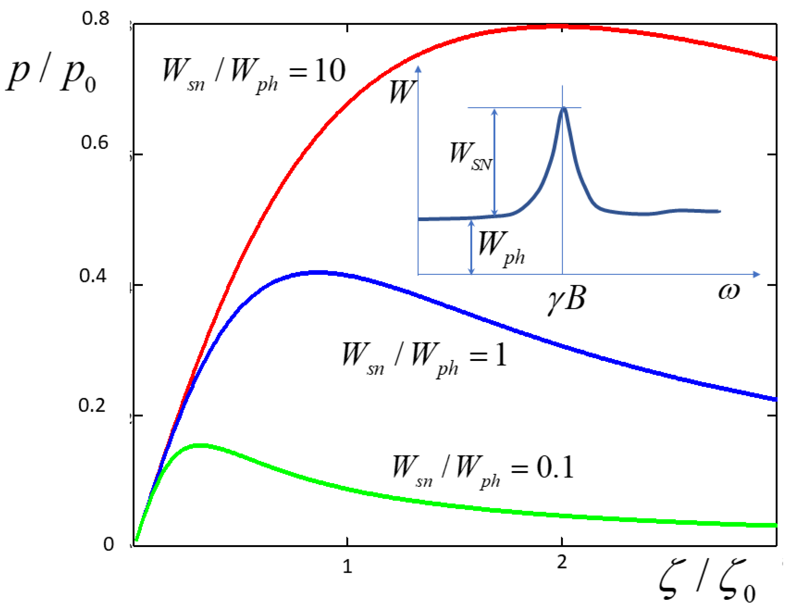
The main limitation of the method comes from the background noise in the optical channel, which, being amplified and converted into the current in the magnetic coil, gives rise to a noise magnetic field that warms up the nuclear spin system. Up-to-date spin noise spectroscopy can successfully fight all sources of noise except the shot noise of photons in the probe beam [6]. This photonic noise results in fluctuations of the Faraday rotation angle with the flat spectral power density inversely proportional to the fluence of the probe beam. A typical spectrum of Faraday rotation noise of a spin system in a transverse magnetic field is shown in the inset to Figure 4.
If the spectral power density (SPD) of photonic noise is , while that of the spin noise at the resonance peak is , transformation of the photonic noise by the circuitry results in the random magnetic field with the SPD equal to
This random field induces depolarization of nuclear spins at the rate
where is given by Eq.(22). Therefore, to take into account spin depolarization, or warm-up, due to the photonic noise, one should replace in Eqs.(19)-(21) with defined as
The dependences of spin polarization on the transformation coefficient for different ratios of spectral power densities of the spin noise and the background photonic noise are plotted in Figure 4. One can see that the warm-up due to the background noise results in a decrease of polarization at large . The polarization that can be reached at optimal rather weakly depends on ; actually it amounts to a considerable fraction of once the spin noise peak is discernible over the photonic noise background.
To estimate the effect in numbers, one needs to consider a specific object. The possibility to detect the nuclear spin fluctuations optically has been already demonstrated experimentally in bulk GaAs [15]. We propose to use GaAs/AlGaAs microcavity structures, which vastly improve the sensitivity of the method [16,17]. In order to estimate the efficiency of nuclear spin cooling by oscillating fields, we assume using of an optical microcavity with a GaAs active layer, similar to one studied in Ref.[14]. With the thickness of the active layer of 0.35 and the beam diameter of 2, the probed volume is approximately 1 and the number of nuclei in the probed volume is . The probe beam makes about 1000 round trips inside the cavity, which results in the effective optical path mm. The Faraday rotation angle , induced by the Overhauser field of nuclear fluctuations, , equals
where the nuclear Verdet constant is mrad/(cm.G) [14]. The mean squared Overhaused field of the projection of the nuclear spin fluctuation on the structure axis Z equals:
where 5.3T is the maximum Overhauser field reached when all the nuclear spins are fully polarized.
Thus, the mean squared fluctuation of the Faraday angle equals
Substituting here the structure parameters, we obtain . The frequency range of the fluctuating Faraday signal induced by nuclear spins is determined by the inverse of the spin-spin relaxation time . The mean squared fluctuation of the polarization plane due to the photonic noise of the probe beam with the intensity J in the frequency band 1/Т2 is
Taking equal these two values, we obtain the light intensity under which the spin noise has the same SPD as the photonic one, , which corresponds, with the photon energy of 1.4 eV, to the probe beam transmitted power of 0.7 mW. This is a realistic value for this kind of experiment.
With the typical seconds, one gets, according to Eq.(21), that corresponds, for , to the maximum polarization and maximum Overhauser field of 80 G. Such effective fields are easily detected and measured with optical methods, e.g. by Faraday rotation [14]. These values of polarization and Overhauser field are reached at , which corresponds to the amplitude of the field about mG.
On the whole, the estimated values of experimental parameters and the expected magnitude of the outcome suggest that observation of the effect in GaAs-based microcavity structures is quite realistic. Using more sophisticated structures, e.g. ones with quantum dots in the microcavity, might further enhance the achievable nuclear spin polarization via reducing the number of spins in the probed volume.
5. Conclusions
We have proposed a theoretical background for development of a new method of nuclear spin cooling, which does not involve dynamic polarization by electrons. In fact, the NSS is cooled by an “optical Maxwell demon”, which monitors nuclear spin fluctuations and controls the external magnetic field in a way to pump energy to NSS or out of it. In one of the considered examples, a net nuclear magnetization is built up along certain direction defined by the experimental geometry, similarly to dynamic polarization by spin-polarized electrons. In the other experimental arrangement, the cooling that is not accompanied by the magnetization build-up, or “true cooling” can be realized. Numerical estimates for a GaAs-based microcavity structure demonstrate feasibility of the proposed method. The efficiency of spin cooling can be enhanced by using a quantum dot structure with the reduced total number of nuclear spins.
Author Contributions
Conceptualization, methodology, software, validation, formal analysis, investigation, acquisition, data curation, writing—original draft preparation, writing—review and editing, visualization, supervision, project administration, funding acquisition, K.V.K. All authors have read and agreed to the published version of the manuscript.
Funding
This work was supported by Russian Science Foundation, grant number 22-42-09020.
Acknowledgments
The author thanks D.S.Smirnov for fruitful discussions.
Conflicts of Interest
The authors declare no conflict of interest. The funders had no role in the design of the study; in the collection, analyses, or interpretation of data; in the writing of the manuscript; or in the decision to publish the results.
References
- Abragam, A. The Principles of Nuclear Magnetism; Clarendon Press: Oxford, 1961. [Google Scholar]
- Goldman, M. Spin Temperature and Nuclear Magnetic Resonance in Solids— International Series of Monographs on Physics; Clarendon: Oxford, UK, 1970. [Google Scholar]
- Purcell, E.M.; Torrey, H.C.; Pound, R.V. Resonance Absorption by Nuclear Magnetic Moments in a Solid. Phys. Rev. 1946, 69, 37. [Google Scholar] [CrossRef]
- Litvyak, V.M.; Cherbunin, R.V.; Kalevich, V.K.; Lihachev, A.I.; Nashchekin, A.V.; Vladimirova, M.; Kavokin, K.V. Warm-up spectroscopy of quadrupole-split nuclear spins in n-GaAs epitaxial layers. Phys. Rev. B 2021, 104, 235201. [Google Scholar] [CrossRef]
- Landau, L.D.; Lifshitz, E.M. Statistical Physics, 3rd ed.; Butterworth-Heinemann: Oxford, 1980. [Google Scholar]
- Zapasskii, V.S. Spin-noise spectroscopy: from proof of principle to applications. Advances in Optics and Photonics 2013, 5, 131–168. [Google Scholar] [CrossRef]
- Dyakonov, M.I. Spin Physics in Semiconductors, 2nd ed.; Springer Series in Solid-State Sciences Vol. 157; Springer: Berlin, 2017. [Google Scholar]
- Vladimirova, M.; Cronenberger, S.; Colombier, A.; Scalbert, D.; Litvyak, V.M.; Kavokin, K.V.; Lemai, A. Simultaneous measurements of nuclear-spin heat capacity, temperature, and relaxation in GaAs microstructures. Phys. Rev. B 2022, 105, 155305. [Google Scholar] [CrossRef]
- Flisinski, K.; Gerlovin, I.Y.; Ignatiev, I.V.; Petrov, M.Y.; Yu, S.; Yakovlev, D.R.; Reuter, D.; Wieck, A.D.; Bayer, M. Optically detected magnetic resonance at the quadrupole-split nuclear states in (In,Ga)As/GaAs quantum dots. Phys. Rev. B 2010, 82, 081308(R). [Google Scholar] [CrossRef]
- Chekhovich, E.A.; Kavokin, K.V.; Puebla, J.; Krysa, A.B.; Hopkinson, M.; Andreev, A.D.; Sanchez, A.M.; Beanland, R.; Skolnick, M.S.; Tartakovskii, A.I. Structural analysis of strained quantum dots using nuclear magnetic resonance. Nat. Nanotechnol. 2012, 7, 646. [Google Scholar] [CrossRef] [PubMed]
- Dzhioev, R.I.; Korenev, V.L. Stabilization of the electron-nuclear spin orientation in quantum dots by the nuclear quadrupole interaction. Phys. Rev. Lett. 2007, 99, 037401. [Google Scholar] [CrossRef] [PubMed]
- Meier, F.; Zakharchenja, B.P. (Eds.) Optical Orientation; North-Holland: Amsterdam, 1984. [Google Scholar]
- Vladimirova, M.; Cronenberger, S.; Scalbert, D.; Ryzhov, I.I.; Zapasskii, V.S.; Kozlov, G.G.; Lemaître, A.; Kavokin, K.V. Spin temperature concept verified by optical magnetometry of nuclear spins. Phys. Rev. B 2018, 97, 041301(R). [Google Scholar] [CrossRef]
- Giri, R.; Cronenberger, S.; Glazov, M.M.; Kavokin, K.V.; Lemaître, A.; Bloch, J.; Vladimirova, M.; Scalbert, D. Nondestructive Measurement of Nuclear Magnetization by Off-Resonant Faraday Rotation. Phys. Rev. Lett. 2013, 111, 087603. [Google Scholar] [CrossRef] [PubMed]
- Berski, F.; Hübner, J.; Oestreich, M.; Ludwig, A.; Wieck, A.D.; Glazov, M. Interplay of Electron and Nuclear Spin Noise in n-Type GaAs. Phys. Rev. Lett. 2015, 115, 176601. [Google Scholar] [CrossRef] [PubMed]
- Ryzhov, I.I.; Poltavtsev, S.V.; Kavokin, K.V.; Glazov, M.M.; Kozlov, G.G.; Vladimirova, M.; Scalbert, D.; Cronenberger, S.; Kavokin, A.V.; Lemaître, A.; Bloch, J.; Zapasskii, V.S. Measurements of nuclear spin dynamics by spin-noise spectroscopy. Appl. Phys. Lett. 2015, 106, 242405. [Google Scholar] [CrossRef]
- Ryzhov, I.I.; Kozlov, G.G.; Smirnov, D.S.; Glazov, M.M.; Efimov, Y.P.; Eliseev, S.A.; Lovtcius, V.A.; Petrov, V.V.; Kavokin, K.V.; Kavokin, A.V.; Zapasskii, V.S. Spin noise explores local magnetic fields in a semiconductor. Sci. Rep. 2016, 6, 21062. [Google Scholar] [CrossRef] [PubMed]
Figure 1.
Scheme of the experiment on dynamic spin polarization in a constant magnetic field perpendicular to the structure axis. Red arrow shows the direction of the probe beam of linearly polarized light with the fluence J. Fluctuations of its polarization plane induced by spin fluctuations in the sample, detected with the polarimetric device, form the spin noise signal used to control the current in the magnetic coil that creates the time-dependent magnetic field .
Figure 1.
Scheme of the experiment on dynamic spin polarization in a constant magnetic field perpendicular to the structure axis. Red arrow shows the direction of the probe beam of linearly polarized light with the fluence J. Fluctuations of its polarization plane induced by spin fluctuations in the sample, detected with the polarimetric device, form the spin noise signal used to control the current in the magnetic coil that creates the time-dependent magnetic field .
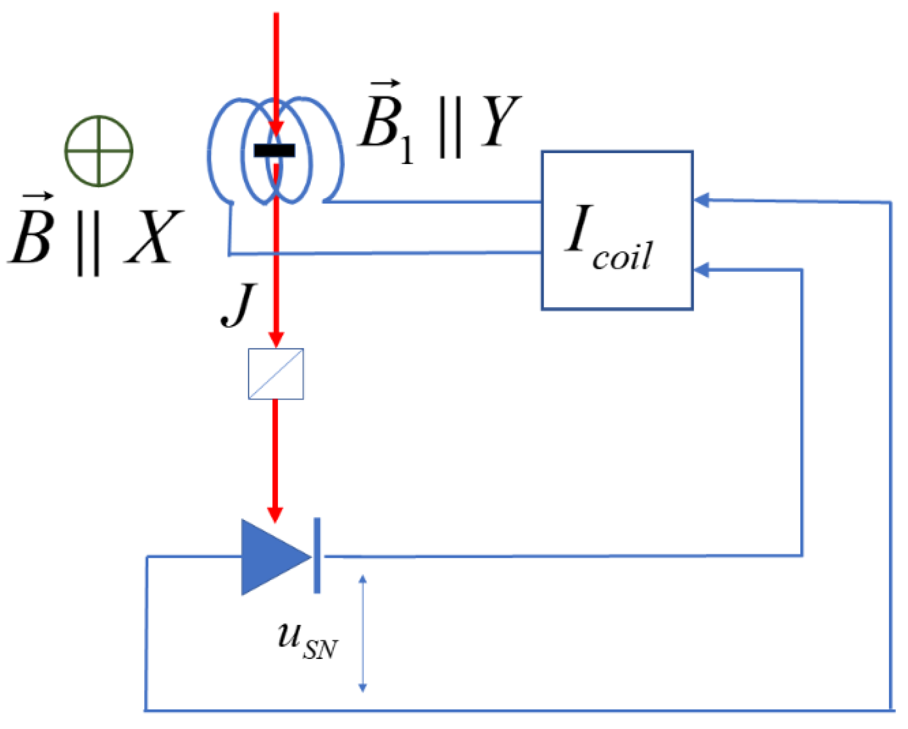
Figure 2.
Schematic explanation of the dynamics of the nuclear magnetic moment under the magnetic field , correlated with the nuclear spin fluctuation. The field turns the Y-component of the fluctuating part of nuclear magnetic moment so that it feeds the regular magnetization along X. At the same time, turns in the XY plane so that decreases.
Figure 2.
Schematic explanation of the dynamics of the nuclear magnetic moment under the magnetic field , correlated with the nuclear spin fluctuation. The field turns the Y-component of the fluctuating part of nuclear magnetic moment so that it feeds the regular magnetization along X. At the same time, turns in the XY plane so that decreases.
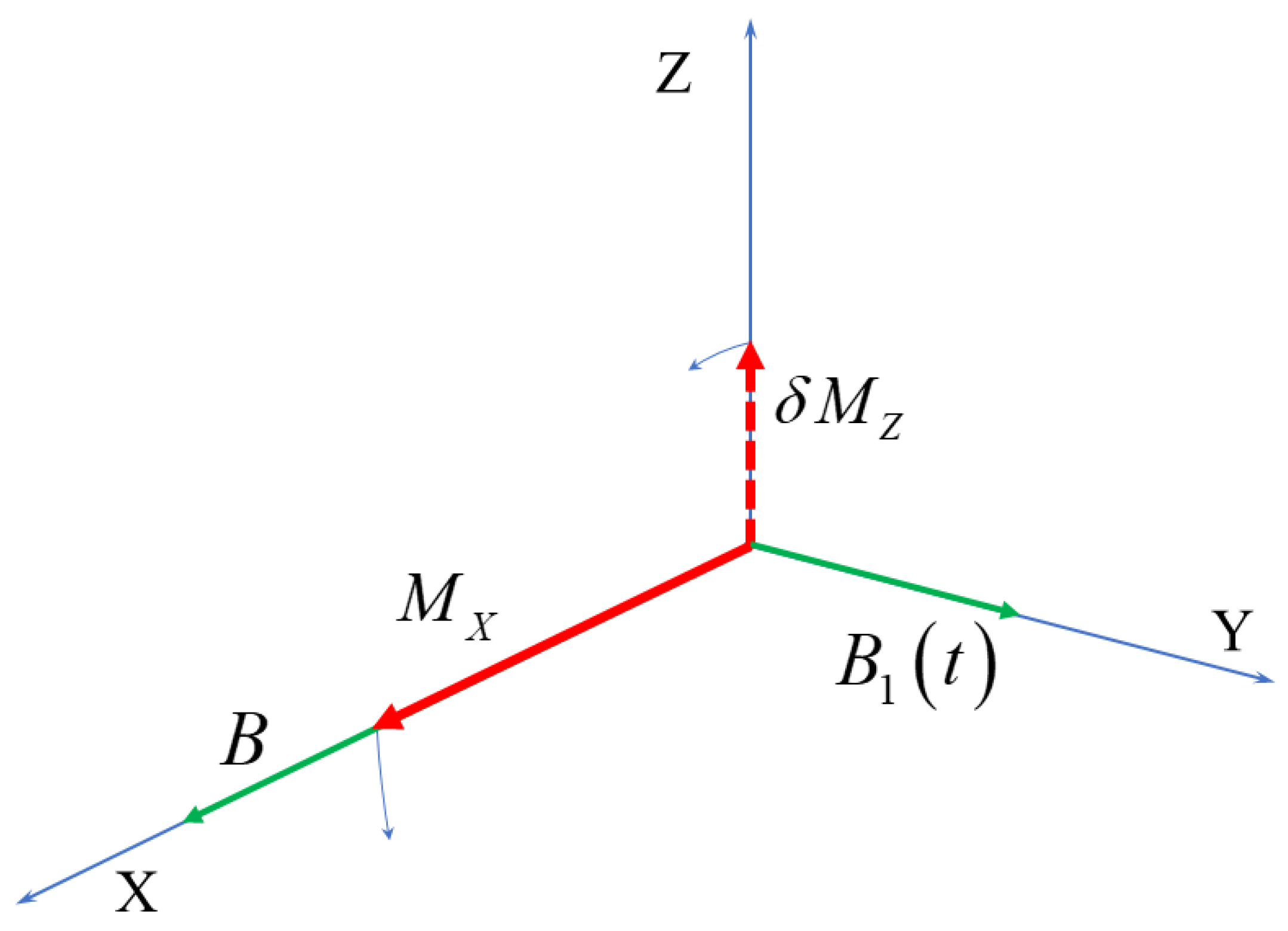
Figure 3.
Experimental arrangement for “true” nuclear spin cooling in external field. The time-dependent field is applied parallel to the probe beam, with the phase shift between the field and the optical spin noise signal being provided by the electronics.
Figure 3.
Experimental arrangement for “true” nuclear spin cooling in external field. The time-dependent field is applied parallel to the probe beam, with the phase shift between the field and the optical spin noise signal being provided by the electronics.
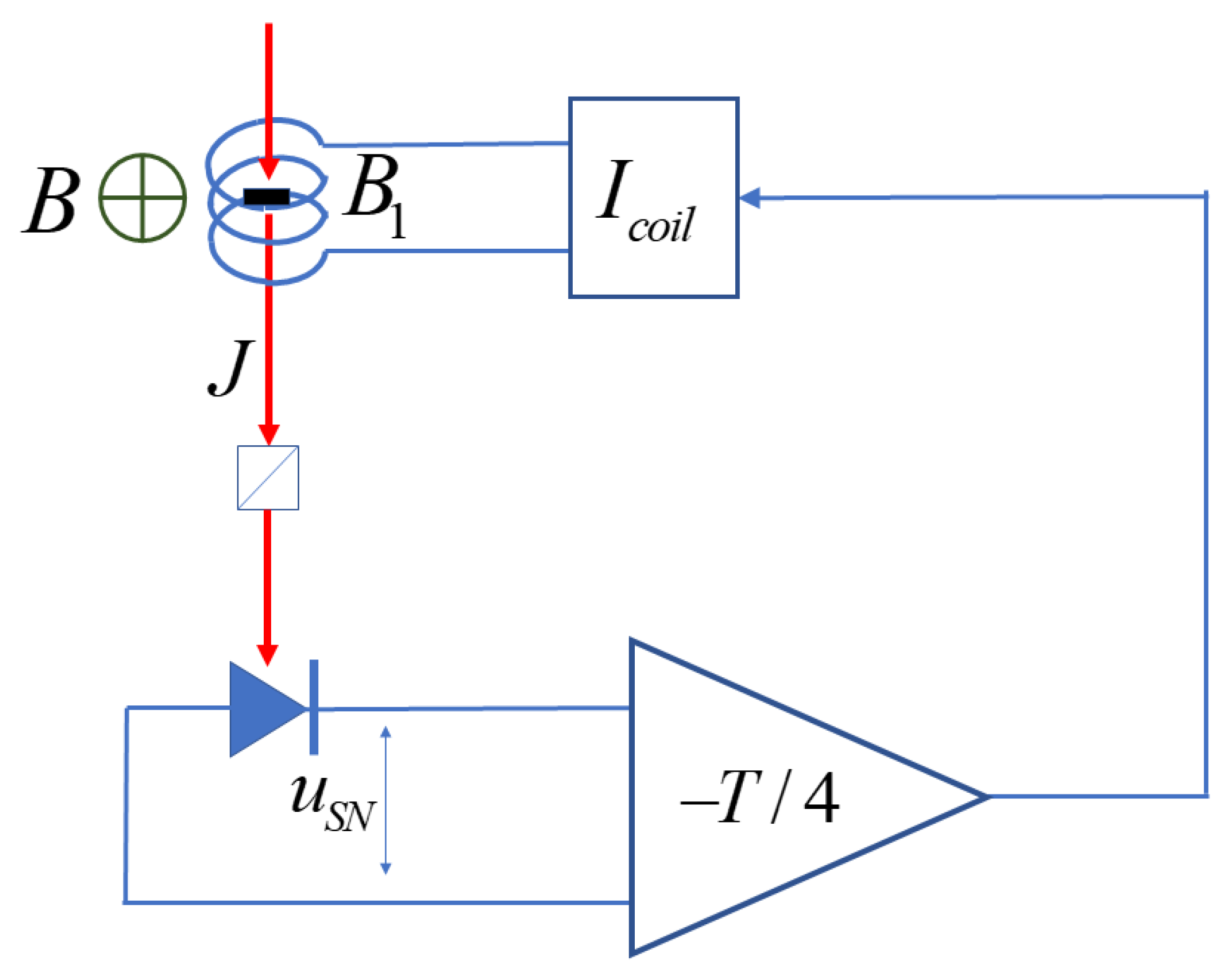
Figure 4.
Spin polarization vs the transformation coefficient for different ratios of spectral power densities of spin noise (at the peak) and of background photonic noise . Inset: typical spectrum of spin noise in a transverse magnetic field over the background of photonic noise.
Figure 4.
Spin polarization vs the transformation coefficient for different ratios of spectral power densities of spin noise (at the peak) and of background photonic noise . Inset: typical spectrum of spin noise in a transverse magnetic field over the background of photonic noise.
Disclaimer/Publisher’s Note: The statements, opinions and data contained in all publications are solely those of the individual author(s) and contributor(s) and not of MDPI and/or the editor(s). MDPI and/or the editor(s) disclaim responsibility for any injury to people or property resulting from any ideas, methods, instructions or products referred to in the content. |
© 2023 by the authors. Licensee MDPI, Basel, Switzerland. This article is an open access article distributed under the terms and conditions of the Creative Commons Attribution (CC BY) license (http://creativecommons.org/licenses/by/4.0/).
Copyright: This open access article is published under a Creative Commons CC BY 4.0 license, which permit the free download, distribution, and reuse, provided that the author and preprint are cited in any reuse.


