Submitted:
05 June 2023
Posted:
05 June 2023
You are already at the latest version
Abstract
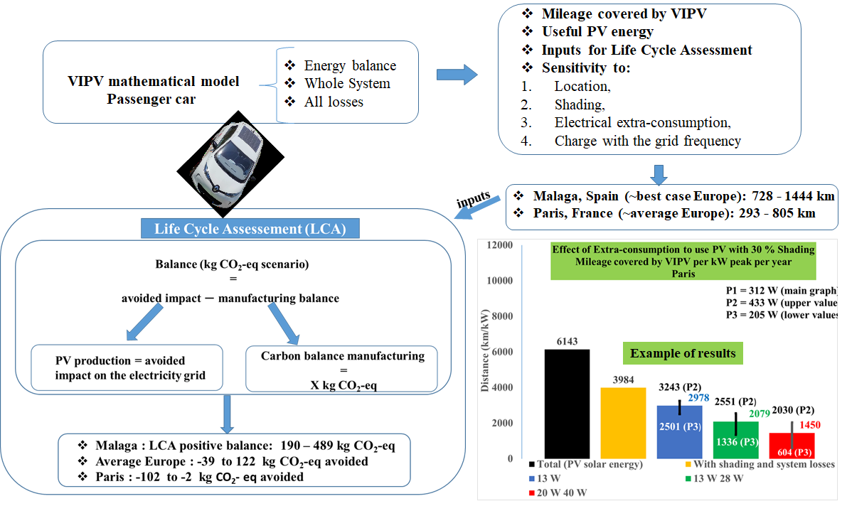
Among the explored solutions to reduce the environmental impact of the transport sector, Vehicle Integrated Photovoltaics. Thus, we developed a simulation tool of the distance covered by VIPV. It considers various usage patterns and vehicle types, several characteristics of the PV system and all the losses that may decrease energy yield. Focusing on passenger car, simulations indicate the order of influence of the parameters on the outputs of the model: geographic locality, shading, thresholds due to extra-consumption to charge the vehicle battery from PV and frequency of recharge with the grid. With projections of the technology in 2030, with 30 % shading, VIPV cover up to 1444 km yearly distance. This represents up to 12 % of the driven mileage. For the best month, it can get up to 14 km/day. For average Europe and worst-case conditions, VIPV cover only 293 km per year. Life Cycle Assessment (LCA) of solarized passenger car shows negative balance for low-carbon electricity mix and average solar irradiance. In favorable conditions, the carbon footprint is up to 489 kg CO2-equivalent avoided emissions on 13 years lifespan. Beyond km and LCA focus, VIPV may provide useful functions in non-interconnected zones and for resilience in disaster zones.
Keywords:
VIPV
; passenger car
; life cycle assessment
; mileage
; electrical architecture
; thresholds
; model
; losses
; shading
; carbon footprint
1. Introduction
Many projects on vehicle-integrated photovoltaics (VIPV) have been carried out recently. Commault et al. (2021) [1] show that the number of VIPV projects is increasing, especially car-based ones. They discussed the benefits and weaknesses of several PV cell and module technologies and give recommendations to large-scale applications of such technologies.
We published recently, Karoui et al. (2023) [2], our work on the evaluation of the performances of the integration of a solar roof on electric bus. This work gives the simulation results for two localities: Malaga (best-case Europe) and Paris (average Europe) and with different shading losses and two architecture for using PV. It shows that adding VIPV on a city bus allows covering between 3711 km and 9739 km. Life cycle assessment shows neutral to high gains. The avoided gas emissions are up to 28 T CO2-equivalent on 20 years lifetime. Thiel et al. (2022) [3] estimated the energy performances of solar integration on a personal vehicle and on a distribution van in various climatic conditions without shading. They show that photovoltaics can give up to 35 % of the driven distance. Sagaria et al. [4] study the interactions between solar energy for five categories of vehicle and usage configurations for VIPV. They take into account the shading but only in the sunny city of Lisbon in Portugal.
Other studies include the impact of shading on the performances of VIPV. Lodi et al. (2018) [5] from the European Commission Joint Research Center show that the PV usage factor is 58 % for passenger cars. This study allows the European commission to fix the value of shading losses for eco-innovation to 49 % [6] to extrapolate the results in other locations in Europe. They call it shading share and it is equal to 100 %-PV usage factor, which is equal to 51 %. Arun et al. (2019) [7] studied the influence of partial shading in VIPV systems and the variation of output power with different forms of shading for a car. They simulated the maximum power point tracker (MPPT) using or not a boost converter. Brito et al. (2021) [8] contributed to shading studies giving an average of 52 % irradiance loss during parking of 26 % during driving cycles in urban environment in Lisbon. They calculate an average daily distance covered by VIPV in a year between 10 and 18 km/day/kWp.
For passenger car, there are some losses due to curvature of the solar panel. Ota et al. [9,10] proposed a methodology to characterize commercial solar roof shapes, with a direct link to the potential PV coverage ratio. For a radius of curvature of 1 m, the coverage ratio is 96 %. In this configuration, the curve correction factor to apply is 0.92 for generated energy, compared to a flat module.
The useful energy from VIPV depends also on the frequency of recharge using the grid. Bernie et al. [11] studied the influence of plugin the electric vehicle to the grid in the work place during the hours of daylight. They show that it may induce up to 75 % of loss of the PV available energy from VIPV. Thus, we choose to recharge the vehicle with the grid at night. In our calculations, we will use the frequency of recharge with the grid as a variable parameter.
Finally, the energy loss in electronic components allowing charging the main battery of the vehicle using PV has an influence on the VIPV performance. We have already shown partially this influence for the city bus [2] demonstrating that in this case charging directly PV in the main battery is better that charging first the low voltage battery and periodically transfer energy from low voltage to high voltage battery. We will study in the present paper more deeply this question for passenger car in the Section 3.2.
The authors do not find a previous study, which takes into account all the factors that may influence the performance of VIPV on passenger car. These factors are locations, shading share, charge architecture, power thresholds for using PV, curvature of the solar panel, and frequency of recharge with the grid. We will give the performance of VIPV in term of PV energy supplied to the engine, distance covered by VIPV and CO2 emissions estimated with life cycle assessment (LCA).
This paper contributes to the state of the art by evaluating the performances of VIPV on passenger car in European countries. It considers:
- The daily usage patterns which may vary during the week and the year
- The monthly variations of the solar irradiance and their hourly distribution,
- The PV panel curvature,
- The solar panel ageing,
- The shading,
- The system effectiveness,
- Three architectures to transfer energy from PV to the battery,
- The battery fullness due to the frequency of recharge with the grid and to the rest days.
Energy/distance simulation model gives inputs to life cycle analysis process allowing calculating the carbon avoided emissions.
We structured this article in five sections. In Section 2, we describe the model, data and parameters. Section 3 gives the simulation results with three architectures to transfer energy from the VIPV to the main battery (through 12 V battery, by means of 48 V additional battery and directly in the high voltage battery). In the Section 3.1, we will give the results regarding PV energy transferred to the engine and distance covered by VIPV. In Section 3.2, we will give the results of the parametric study of the combination PV peak power and thresholds for using PV. In Section 3.3, we will give the LCA results. We discuss the obtained results in Section 4. Section 5 is the conclusions of this study.
2. Materials and Methods
Most of the material and methods are common with the e-bus use case that we have described in our paper [2] published in open access. The differences are:
- The curvature losses since passenger car have not a flat panel,
- The influence of frequency of recharge with the grid,
- The Sensitivity analysis regarding the electricity consumption of the electronics and the thresholds to use or not the PV energy,
- Three electrical architectures for charging the battery of passenger car with PV. For the bus, there were only two architectures,
- The parameters of simulations, mainly PV surface, consumption in Wh per km, system efficiency; battery size, shading and use profile,
The Figure 1 gives the inputs, outputs, parameters and the characteristics of the model that calculated the PV energy transferred to the engine and the distance covered by the VIPV.
2.1. Measurement and calculation of losses due to the curvature
We measured the losses due to the curvature in function of the sun elevation at Zenith for two solar panels with different curvatures in Chambéry, France. For this, we did outdoor measurements of the maximum power point on one curved solar roof (radius of curvature near 3 m) and one standard flat reference module. We placed the modules toward south with 0° inclination (horizontally). From August 2019 to February 2020, we did a measurement every 5 minutes on daytime. From this, we computed an approximation of a linear regression of the producible loss versus the flat reference module as a function of the sun elevation at zenith. We extrapolated this regression to compute the curvature losses of each location and according to the sun elevation at zenith through the typical year.
We used the declination of the sun at the 15th of each month in the Equation (1) (Shivalingaswamy et al. [12]) to calculate the sun elevation at Zenith in function of the co-latitude and of the declination of the sun.
Therefore, we calculated the losses due to the curvature at the 15th of each month for each city with the considered solar roofs.
Considering the average and the highest annual PV productions among 19 cities in Europe, we have chosen for VIPV studies the localities of Paris and Malaga as explained in our previous paper [2] (p.3).
The Figure 2 shows the annual PV produced energy in Malaga and Paris in kWh per unit of peak power with and without curvature correction. The total production respectively for flat panel and curved panel is 1635 kWh/kWp and 1535 kWh/kWp in Malaga and is 1058 kWh/kWp and 965 kWh/kWp in Paris. The losses due to curvature are 8.8 % in Paris and 6.1 % in Malaga for a year.
2.2. Electrical architectures, system efficiency and thresholds
In order to charge PV energy in the vehicle battery, we considered three electrical architectures for passenger car. These architectures allow either charging the solar energy directly in the high voltage (HV) battery or charging first a low voltage (LV) battery and then intermittently transmit energy from LV battery into the HV battery.
The additional consumed energy to use PV and the system efficiency depend on the chosen architecture for charge. For direct charge in the HV battery, this consumption is 12 W during driving and during plugin into the grid and 26 W during parking. For charge via low voltage auxiliary battery (12 V or 48 V), this consumption is constant and is 12 W. In this case, there is a periodic wakeup (each 100 Wh) of the vehicle calculators and HV battery management system in order to transmit the electricity from LV battery to HV battery. The consumption is 8.5 Wh per wakeup.
The additional electricity consumption divided by the system efficiency is equal to the thresholds applied to decide to trigger or not the PV use. The system transmits the PV energy to the battery only if the available power during the time step is higher than these thresholds. The model subtracted this additional electricity consumption from the PV produced energy during all computing time steps. We give more details on the thresholds in Section 3.2.1.
The Table 1 gives the efficiency of each component and the total system efficiency for each architecture for passenger car.
2.3. Usage profile and parameters for passenger car
To estimate the consumption per km for passenger car, we used data referenced in the website [13]. The average between the given values is 15.7 kWh/100 km and so 157 Wh/km.
The model utilizes the usage pattern (driving, parking, plugin) to calculate the consumption for all the days and all the computing time steps.
The passenger car is driven for home/work trip: one hour morning (8 am-9 am) and one hour evening (5 pm-6 pm), 5 days per week and 48 weeks per year. Passenger car has thus long parking periods (8 hours per day).
The battery size for passenger car is 50 kWh.
The PV peak power used in the simulations at midlife considers a lifetime of the passenger car of 13 years and a PV degradation of -2 % 1st year then -0.7 % per year. It is measured using INES facilities and is comparable to that reported by Jordan et al. (2016) [14].
We consider two PV surfaces:
- 1.44 m², value corresponding to covering 90 % of the average surface of passenger car roofs in France (1.58 m²). This surface leads to 312 Wp at midlife with projection of the technology in 2030. The simulations in results section will be given with this value of PV surface
- 2 m², value considered by Thiel et al. [3]. We will discuss the effect of such increase in PV surface in Section 4.3.
We evaluate the daily PV producible of the panel with 49 % and 30 % shading factors. The value of 49 % given by the European commission [5] is mandatory to assess the potential of VIPV but includes parking inside. The value of 30 % is calculated using the loss of energy for a year in urban driving environment compared with stationary PV.
2.4. The frequency of recharge with the grid
We consider two frequencies of recharge with the grid: every night before a driving day and the maximal recharge frequency depending on the battery size and on the consumption of the vehicle. We calculate this frequency using the following Equation (2). It is equal to five. Charging every five nights is enough for driving this passenger car for five days.
We calculate the state of charge profile of the battery using the method described in our previous work [2] (p.6). Such calculation allows obtaining the useful PV energy taking into account the influence of battery saturation.
3. Results
This section gives the results of the simulations for Paris (equal to average Europe use case) and Malaga (equal to best use case in Europe) for three architectures of transmission of PV electricity to the battery: directly in the HV battery, through 12 V battery or 48 V battery.
3.1. Results regarding energy and distance covered by VIPV
This subsection treats the simulation results of the energetic mathematical model.
3.1.1. Simulation of the quotidian profiles
Figure 3 shows the electricity consumption and the PV production within ¼ h time step and the state of charge (SOC) for passenger car for two months. The consumption graphs are curtailed in order to zoom on production.
These graphs show that:
- In January, the vehicle does not use the PV energy when it is lower than the thresholds associated with the additional consumption of electricity allowing using PV,
- In June, the PV production is higher than these thresholds but it is not used early in the morning because of the fullness of the battery,
- The SOC profiles depend mostly on the use profile of the vehicle because the consumption is much higher than the production,
- There is a steady increase of the SOC during the night due to recharge with the grid,
- For passenger car, during the parking period, the battery SOC increase is very low even in June.
3.1.2. Available energy from VIPV system
Figure 4 compares the performances of the three techniques to transfer the electricity from the solar roof to the battery of passenger car with three values of shading share. The black column concerns the annual photovoltaic energy correlated only to the solar irradiance in the specific locality. We divided the bar graph into three portions from the left side to the right side: the first one is for charge via 12 V battery, the second one is for transfer through 48 V battery and the third one is for directly charging the HV battery.
The PV energies including the system efficiency are on the yellow columns. They depend simply on the efficiency values given in Table 1. The other bars include the shading share influence and the effect of the thresholds (more detailed in Section 3.2.1). On these bars, we indicate two values according to including or not the losses due to the battery fullness. The battery may be full:
- In the morning before driving due to plugin into the grid at night. We will present the sensitivity of the model to the charge frequency in Figure 5,
- During the rest days because there is no consumption due to the driving
The columns corresponding to shading share 0 % (blue ones) in Figure 4 include the additional electricity consumption to transfer PV energy that varies with the considered architecture and with the daylight duration. It is major relatively to the annual energy presented in the yellow columns. It is 98 kWh (54 %) in Paris and 100 kWh (29 %) in Malaga with direct charge of the HV battery from VIPV system. It is 67 kWh (34 %) in Paris and 80 kWh (24 %) in Malaga for architectures with charge via LV battery. The percentage is relative to PV energy with 0 % shading.
These graphs in Figure 4 show also that:
- The difference of energies between Malaga and Paris is about 70 %. The locality has a the major influence,
- The shading share is the second effect,
- The extra-consumption to use the PV and so the thresholds have third order influence (24 %-54 %) depending on the architecture and the location
- The battery fullness has forth order influence (11 % - 16%).
- The architecture with transfer through 48 V battery is more effective than transfer through 12 V battery, which is more effective than charging directly the HV battery (except with 0 % shading in Malaga). However, its impact is fifth order (difference between architectures is only 7 %). Changing the electrical architecture of recharge has less influence than optimizing the thresholds. As indicated before, we will give a sensitivity study of the influence of the tuple thresholds/peak power in Section 3.2.
The blue bars are for shading equal to zero, which is not realistic in the case of passenger car. Thus, the values up to given are for the green bars that include the system effectiveness, the additional consumption to transfer PV and a representative value of shading share. Readers can refer to the graphs to get the values with 0 % shading. Thus, Figure 4 shows also that:
- For the best-case: Malaga, 30 % shading, charging through 48 V battery and when battery is never full, the passenger car can gather up to 227 kWh.
- In Paris (~average Europe), passenger car can gather up to 126 kWh with 30 % shading, when charging through the 48 V battery and when battery is never full and down to 46 kWh with 49 % shading with charging with PV directly the HV battery and with battery fullness.
Figure 5 presents the sensitivity of the model to the frequency of recharge for the case of direct transfer of the PV energy in the HV battery.
Figure 5 shows that the effect of frequency of recharge is small, compared to other parameters. The difference between recharging with the grid every night and every five nights is 5 % in Malaga and 12 % in Paris with 30 % shading share.
3.1.3. Yearly distance covered by VIPV
Figure 6 presents the Yearly distance covered by VIPV system on a passenger car for the three architectures to transfer the PV energy into the HV battery.
Figure 6 shows that VIPV can generate up to 1444 km per year at midlife in Malaga with 30 % shading share and with transfer of energy through 48 V battery. This distance represents 12 % of the driven mileage (12250 km). The range extending is down to 293 km per year in Paris with 49 % shading share, direct charge of HV battery and with battery fullness losses. It represents about 2 % of the driven mileage. If we normalize the results with the peak power of the solar roof, the annual mileage covered by the VIPV is up to 4628 km/kWp and down to 939 km/kWp.
Figure 7 presents the simulation results regarding the influence of the frequency of recharge for the case of directly charging HV battery on the yearly distance covered by VIPV. It shows that charging the battery with the maximal charging frequency (every 5 nights) allows obtaining between 36 km and 151 km more than charging every night.
3.1.4. Daily distance covered by VIPV
Figure 8 presents the simulated average daily distance by VIPV on passenger car for the three architectures of energy transfer. These values take into account battery saturation. When analyzing daily distance, we can give values up to without shading losses.
Figure 8 indicates that for June, the sunniest month, the VIPV at midlife can cover an average distance up to 14 km/day (44 km/day/kWp) in Malaga, shading 0 % and directly charging the main battery. The difference between architectures of energy transfer is less than 1 km.
It shows moreover that in Paris (~ average Europe), the VIPV can cover up to 8.7 km with 0 % shading and down to 3.3 km with 49 % shading.
3.2. Parametric study of the tuple PV peak power/thresholds related to electrical architecture
3.2.1. Values of the thresholds
In VIPV application, PV energy has to be managed all the time that means during parking and driving phases. Due to vehicle electrical architecture, safety, or energy management reasons, dedicated electromechanical elements, Electronic Control Unit (ECU), or Battery Management System (BMS) has to be switched-on to manage the energy flow from PV panels to the battery. It results on power threshold values at system level: below these values, the PV power from the panel is not available, due to a negative energy balance at system level. In this context, we consider three use cases in our energy predictions:
- 13 W during driving and parking phases. This is the most optimist hypothesis (only electromechanical relay on main battery)
- 13 W during driving and recharge with the grid phases and 28 W during parking phase. This is the realistic hypothesis. During parking phase, a partial wakeup is needed, which results in 28 W
- 20 W during driving and charge with the grid phases and 40 W during parking phase. These values were measured on a commercial electrical vehicle including VIPV.
We will study these three use cases to compare the energy performances and losses at vehicle level.
Figure 9 presents an explanation of the thresholds effect.
3.2.2. Analysis of the combination peak power/thresholds
We simulate the effect of these thresholds with 30 % shading and with 3 values of peak power 312 W, 433 W and 205 W and without battery saturation.
Figure 10 presents the simulation results for the cities of Malaga and Paris. For the calculation of the losses, the reference is the yellow bar including the system efficiency and shading effects.
Figure 10 shows that:
- Lower peak power induces bigger losses of PV energy and distance due to thresholds. Therefore, even if the graphs present the distance per kW peak, the values are different in function of peak power.
- The losses due to thresholds are very high. The minimum is 12 % (Malaga, 433 W peak, threshold 13 W) and the maximum is 85 % (Paris, 205 W peak, thresholds 20 W and 40 W).
- With the same shading level, the percentage of use of the PV depends on the location (1st order), the thresholds (2nd order) and the peak power (3rd order).
- The mileage covered by VIPV per unit of peak power in Malaga is up to 5569 km/kW and down to 2218 km/kW depending on the peak power and the thresholds values.
- The distance covered by VIPV per unit of peak power in Paris is up to 3243 km/kW and down to 604 km/kW depending on the peak power and the thresholds values.
We calculate that with thresholds equal to 13 W and 28 W, a peak power of 131 W can cover only the losses in Paris, without generating distance.
3.3. Life Cycle assessment results
We described the methodology of life cycle assessment in our paper regarding the city bus use-case [2] (pp. 7-10). It is common to passenger car. We remind here that we take into account a low-carbon PV panel and that we do not consider the end of life of the PV system. The main differences are the parameters regarding the PV surface and so the additional weight, the life duration of the vehicle and the additional battery in the case of charge via 48 V battery.
3.3.1. Details of the fabrication phase
Table 2 presents the results of the fabrication phase for the three architectures.
3.3.2. Carbon footprint results
The estimation of the carbon footprint takes into account the fabrication and usage phases of the vehicle. Regarding usage periods, we give the results with different localities according to electricity mix and solar irradiance: Malaga, average Europe and Paris. We consider a global warming scenario set at +2.7 °C.
The Figure 11, Figure 12 and Figure 13 present life cycle assessment results. In each figure, the panel on the left is for the three architectures of charge with different shading levels. The panel on the right presents the effect of frequency of recharge with the grid for the architecture with directly transmission of the electricity in the HV battery with different shading values.
Figure 11, Figure 12 and Figure 13 show that in the case of passenger car, VIPV may have a positive balance but not in all localities. The CO2 balance depends mainly on the locality. With a very low-carbon electricity mix in France, VIPV on passenger car is not convincing. It has a negative CO2 balance in Paris with 30 % and 49 % shading losses between -2 and -102 kg CO2-eq. In best-case in Europe, it permits avoiding up to 489 kg CO2-eq (Malaga, 30 % shading and charge through 12 V battery). For average Europe in term of electricity mix and solar irradiance, VIPV may be not interesting because avoided emissions are 122 kg CO2-eq in the best conditions (30 % shading, charge through 12 V battery) and -39 kg CO2-eq in worst conditions.
4. Discussion
The vehicle constructer can improve the consumption of the vehicle per km, the additional consumption for delivering the PV electricity to the battery (and so the related thresholds), the architecture for electricity transfer and the PV peak power.
The car driver can optimize the PV usage by recharging less frequently with the grid and of course parking the vehicle preferably in sunny places.
Henceforward, we discuss the impact on the simulation results of considering variable shading losses instead of constant shading losses, a bigger surface of the PV and a lower system efficiency. Finally, we will present a case study with an optimized PV surface and energy consumption per km.
4.1. Variable shading vs constant shading
We compare here a constant shading value during a year with a variable value of shading between months with higher shading during winter compared to summer. These values of shading induce a loss for one year in Paris of 30 % of the PV energy. The values are estimated by modelling with 10 m height buildings and with 11 m of route width in urban environment. M.C. Brito et al. [8] explained the variation of shading losses during a year saying that the lower solar elevation in winter induces higher losses due to shading from buildings. Table 3 gives the shading values for the months of a year in Paris. The values are between 21 % and 69 %.
The Table 4 presents the simulation results with variable shading between months compared to a constant shading in Paris. It shows an improvement between 0 % and 9 % of the used energy and of the distance covered by VIPV. The improvement is only between 1 and 2 kg CO2-eq when we look at life cycle assessment results.
Another possibility to take into account the shading is to consider different values between driving and parking. We have simulated the use cases with shading losses equal to 26 % during driving and 52 % during parking, which are average year values for road and parking given by M. C. Brito et al. [8].
The Table 5 presents the simulation results with different shading between driving and parking compared to constant shading of 49 % in Paris and Malaga for the three electrical architectures. We give the energies for a charge with the grid every five nights.
This table shows small influence for considering different shading losses between driving and parking phases. This is because the usage profile of passenger cars includes parking most of the day.
4.2. Consequence of lower system efficiency
The Table 6 presents the evolution of the used PV energy if the system effectiveness is lower than that used in our projections.
It indicates that the influence is not linear. When the system efficiency is 13 % lower, the PV energy used by the engine decreases between 20 % and 25 %. A 23 % drop of such efficiency makes the energy decreasing between 36 %-45 %
The difference between passenger car and city bus (our previous paper [2]: the influence for city bus is almost linear) is the relatively high influence of the thresholds to trigger or not the transfer of PV energy. This is because the parking period is longer and the produced energy is much lower for passenger car than that for city bus.
4.3. Influence of PV surface increase
We considered, for all simulations above, 1.44 m² of solar roof surface. We think that car manufacturers may increase this surface in the future if they prefer to use the solar roofs only on sedans with bigger roof instead of all passenger car vehicles. Thus, we simulate the effect of the solar roof surface increase to 2 m². Thiel from the JRC et al. considers this second value in the reference [3] as a solar roof surface for passenger cars. Thus, we simulate all passenger car electric architectures and use cases with 2 m² solar roof surface as well.
The Table 7 summarizes the results of simulation with both solar roof surfaces.
It shows that such increase of the surface induces an increase of the peak power of 39 %. This leads to 31 % increase of the max values of the PV useful energy and yearly distance covered by VIPV per year and 47 % when we consider min values. For the best month, the increase of the surface leads to 33 % of increase of the max value and 39 % increase of the min value.
With 2 m² solar roof, for the best-case in Europe (Malaga, 30 % shading, architecture of energy transfer through 48 V battery and without battery fullness losses), the driver gets 2078 km per year at midlife of the vehicle, which represents 17 % of the driven distance during a year. When we consider the value of auto-generated distance for the best month: ~ 21 km in this best case, the driver has almost 42 % of the daily distance (~50 km).
4.4. Simulation of the Lightyear use case
We have seen many factors that can influence the performances and gains obtained with a VIPV system on passenger car. We have seen also low performances for the existing vehicles with high level of consumption per km and high influence of the thresholds due to extra-consumption to charge PV energy in the battery. It is interesting here to simulate a use case with a reduction of the consumption per km, with a big surface of PV and with a low consumption of the electrical architecture compared to PV installed power. For this, we take into account the consumption of the vehicle Lightyear 0 [15] that is equal to 109 Wh/km. The battery size of this vehicle is 60 kWh and the solar roof peak power is 1.05 kW. In order to compare with the simulation results above, we consider the three shading levels 0 %, 30 % and 49 % and the three electrical architectures for charging the battery with the PV.
First, we have compared the annual energies normalized for 1 kW at midlife between the vehicle with 0.312 kWp and Lightyear 0. We remind here that the previous vehicle is a solarized electric vehicle, which have the characteristics of average existing electric vehicles in term of consumption (157 Wh/km) and roof surface (1.44 m²) and battery size (50 kWh). Solarizing here means adding a solar system to an existing electric vehicle model. The Lightyear 0 is a vehicle that integrated solar since its conception. We calculate the maximal frequency of recharge with the grid using the Equation (2) in Section 2.4 and we obtain eight. Thus, the model considers a charge with the grid only every eight nights. For the case of average solarized electric vehicle, the considered charge with the grid is every five nights. The Table 8 gives the results of the comparison.
This table shows that the evolution of the useful energy is not linear. It is due to the thresholds related to extra consumption of the vehicle to use the PV energy as explained in 3.2. The higher peak power can even double the useful energy per kWp in the case of high shading level and directly charging the HV battery.
Figure 14 gives the yearly distance covered by VIPV in Paris for a solar vehicle with the main characteristics of Lightyear 0 in term of solar roof peak power, energy consumption per km and battery nominal energy and with recharge with the grid every eight nights.
This figure shows that the values are much higher than that of a solarized electric vehicle. In the worst case in term of shading level and in average Europe in term of irradiance, the solar electric vehicle with the characteristics of Lightyear 0 can cover 2888 km. This is due to cumulated effect of high peak power, which is discussed above, and of a low consumption per km. Unfortunately, the company declared bankruptcy in January 2023. We suppose that it is due to high price (€250, 000) and small production volume. Solarizing existing electrical vehicles has the advantage of affordable cost and the inconvenient of low performances. Affordable cost in the case of solarized vehicles allows higher selling volumes. Therefore, we multiply the carbon footprint by a big number of vehicles and the balance is positive in case of favorable conditions.
5. Conclusions
We analyzed the performances of VIPV on passenger car. We considered three systems to transfer the energy from VIPV to the battery: system with charging directly the HV battery, systems with charging 12 V or 48 V battery before intermittent transmission of the electricity in the HV battery.
Simulations indicate the order of influence of the parameters on the outputs of the model: geographic locality (1st order), shading (2nd order), thresholds related to extra-consumption of VIPV system (3rd order), frequency of recharge with the grid (4th order) and the electric architecture (5th order). System with charging through 48 V battery allows getting higher mileage but has lower performance in term of carbon footprint due to the additional battery. Direct charge of the HV battery may be a compromise between performances in term of mileage, complexity and carbon balance. In Europe, VIPV on passenger car can gather up to 227 kWh per year at midlife with 30 % shading. Thus, it covers up to 1444 km annual distance. This represents 12 % of vehicle needs. For the best month, it can cover up to 14 km per day. For average Europe, in the worst conditions, a passenger car can gather down to 46 kWh per year, which covers 293 km yearly distance.
Based on yearly PV energy and mileage covered by VIPV, life cycle assessment is carried-out. The electricity mix and the solar irradiance have a high impact. With a low-carbon panel, we expect negative balance in term of avoided CO2 in low-carbon electricity mix locations. The balance is positive in favorable conditions (up to 489 kg CO2-eq). Beyond auto-generated distance and LCA topics, VIPV on passenger car could be useful in specific applications, like non-interconnected zones and for resilience in case of naturel catastrophes as indicated by Araki et al. (2023) [17].
Author Contributions
Conceptualization, Fathia Karoui and Bertrand Chambion; Data curation, Fathia Karoui and Fabrice Claudon; Formal analysis, Fathia Karoui and Fabrice Claudon; Funding acquisition, Bertrand Chambion and Benjamin Commault; Investigation, Fathia Karoui; Methodology, Fathia Karoui, Bertrand Chambion, Fabrice Claudon and Benjamin Commault; Project administration, Bertrand Chambion; Resources, Fathia Karoui and Bertrand Chambion; Software, Fathia Karoui; Supervision, Fathia Karoui and Bertrand Chambion; Validation, Fathia Karoui; Visualization, Fathia Karoui; Writing – original draft, Fathia Karoui, Bertrand Chambion, Fabrice Claudon and Benjamin Commault; Writing – review & editing, Fathia Karoui.
Funding
This research received funding from ADEME, grant number 1905C0043. This project was realized with the participation from members of INES.2S and received funding from the French State under its investment for the future program with reference ANR-10-IEED-0014-01
Data Availability Statement
The data presented in this study are available on request from the corresponding author. The data are not publicly available online due to privacy.
Acknowledgments
Authors acknowledge the contributions of Stéphane Cattelani (System efficiency calculation); Nouha Gazbour (Life Cycle Assessment Expert) and Stéphane Guillerez (PV producible) from CEA; Arnaud Richard, Jean-Yves Stineau and Guy Thivin from RENAULT (electronics); Jacques Roux-Michollet and Albert Tienou from SEGULA (variable shading modelling) and Ghazi Jad from FEV (measurements on commercial vehicle)
Conflicts of Interest
The authors declare no conflict of interest.
Abbreviations
The following abbreviations are used in this manuscript:
| BOL | Beginning of Life |
| BMS | Battery Management System |
| ECU | Energy Control Unit |
| HV | High Voltage |
| JRC | European Commission Joint Research Centre ( |
| LCA | Life Cycle Assessment |
| LV | Low Voltage |
| CO2-eq | Carbon Dioxide Equivalent |
| PV | Photovoltaics |
| SOC | State of Charge |
| VIPV | Vehicle Integrated Photovoltaics |
References
- Commault, B.; Duigou, T.; Maneval, V.; Gaume, J.; Chabuel, F.; Voroshazi, E. Overview and Perspectives for Vehicle-Integrated Photovoltaics. Applied Sciences 2021, 11, 11598. [Google Scholar] [CrossRef]
- Karoui, F.; Claudon, F.; Chambion, B.; Catellani, S.; Commault, B. Estimation of Integrated Photovoltaics Potential for Solar City Bus in Different Climate Conditions in Europe. J. Phys.: Conf. Ser. 2023, 2454, 012007. [Google Scholar] [CrossRef]
- Thiel, C.; Gracia Amillo, A.; Tansini, A.; Tsakalidis, A.; Fontaras, G.; Dunlop, E.; Taylor, N.; Jäger-Waldau, A.; Araki, K.; Nishioka, K.; Ota, Y.; Yamaguchi, M. Impact of Climatic Conditions on Prospects for Integrated Photovoltaics in Electric Vehicles. Renewable and Sustainable Energy Reviews 2022, 158, 112109. [Google Scholar] [CrossRef]
- Sagaria, S.; Duarte, G.; Neves, D.; Baptista, P. Photovoltaic Integrated Electric Vehicles: Assessment of Synergies between Solar Energy, Vehicle Types and Usage Patterns. Journal of Cleaner Production 2022, 348, 131402. [Google Scholar] [CrossRef]
- Lodi, C.; Seitsonen, A.; Paffumi, E.; De Gennaro, M.; Huld, T.; Malfettani, S. Reducing CO2 Emissions of Conventional Fuel Cars by Vehicle Photovoltaic Roofs. Transportation Research Part D: Transport and Environment 2018, 59, 313–324. [Google Scholar] [CrossRef]
- Commission Implementing decision of 18 November 2014. Available online: https://eur-lex.europa.eu/legal-content/EN/TXT/PDF/?uri=CELEX:32014D0806&rid=1 (accessed on 4 April 2023).
- Arun, P.; Mohanrajan, S. Effect of Partial Shading on Vehicle Integrated PV System. In the proceedings of the 3rd International conference on Electronics, Communication and Aerospace Technology (ICECA); Coimbatore, India, 12-14 June 2019; in IEEE pp 1262–1267. 14 June. [CrossRef]
- Brito, C-M. ; Santos, T.; Moura, F.; Pera, D.; Rocha, J. Urban Solar Potential for Vehicle Integrated Photovoltaics. Transportation Research Part D: Transport and Environment 2021, 94, 102810. [Google Scholar] [CrossRef]
- Ota, Y.; Araki, K.; Nagaoka, A.; Nishioka, K. Curve Correction of Vehicle-Integrated Photovoltaics Using Statistics on Commercial Car Bodies. Progress in Photovoltaics: Research and Applications 2022, 30, 152–163. [Google Scholar] [CrossRef]
- Ota, Y.; Araki, K.; Nagaoka, A.; Nishioka, K. Facilitating Vehicle-Integrated Photovoltaics by Considering the Radius of Curvature of the Roof Surface for Solar Cell Coverage. Cleaner Engineering and Technology 2022, 7, 100446. [Google Scholar] [CrossRef]
- Birnie, D. P. Analysis of Energy Capture by Vehicle Solar Roofs in Conjunction with Workplace Plug-in Charging. Solar Energy 2016, 125, 219–226. [Google Scholar] [CrossRef]
- Shivalingaswamy, T.; Kagali, B. A. Determination of the Declination of the Sun on a Given Day. European Journal of Physics Education 2012, 3. [Google Scholar]
- Hello Watt. Available online: https://www.hellowatt.fr/suivi-consommation-energie/consommation-electrique/consommation-recharge-voiture-electrique (accessed on 15 November 2021).
- Jordan, D. C.; Kurtz, S. R.; VanSant, K.; Newmiller, J. Compendium of Photovoltaic Degradation Rates. Prog. Photovolt: Res. Appl. 2016, 24, 978–989. [Google Scholar] [CrossRef]
- EV-data base. Available online: https://ev-database.org/car/1166/Lightyear-0 (accessed on 15 may 2023).
- Carexpert. Available online: https://www.carexpert.com.au/car-news/lightyear-solar-powered-ev-enters-production (accessed on 15 may 2023).
- Araki, K.; Ota, Y.; Maeda, A.; Kumano, M.; Nishioka, K. Solar Electric Vehicles as Energy Sources in Disaster Zones: Physical and Social Factors. Energies 2023, 16, 3580. [Google Scholar] [CrossRef]
Figure 1.
Energy and distance modeling.
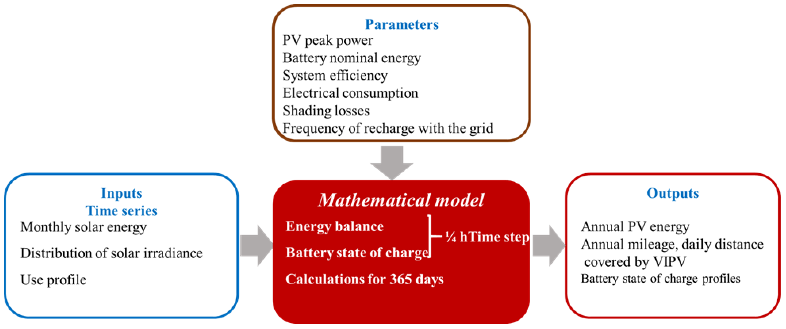
Figure 2.
PV monthly production for 1 kWp for Paris and Malaga.
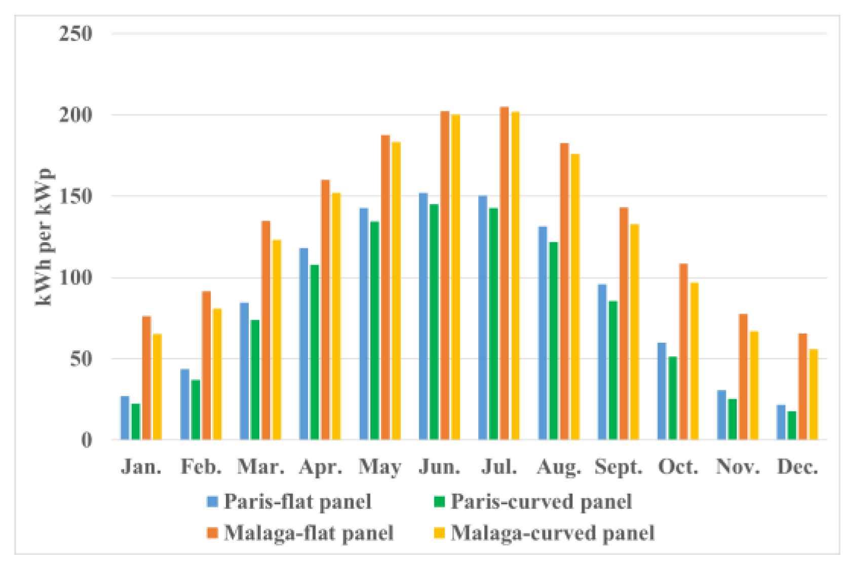
Figure 3.
Examples of profiles, passenger car, direct charge in HV battery, Malaga, shading 30 %.
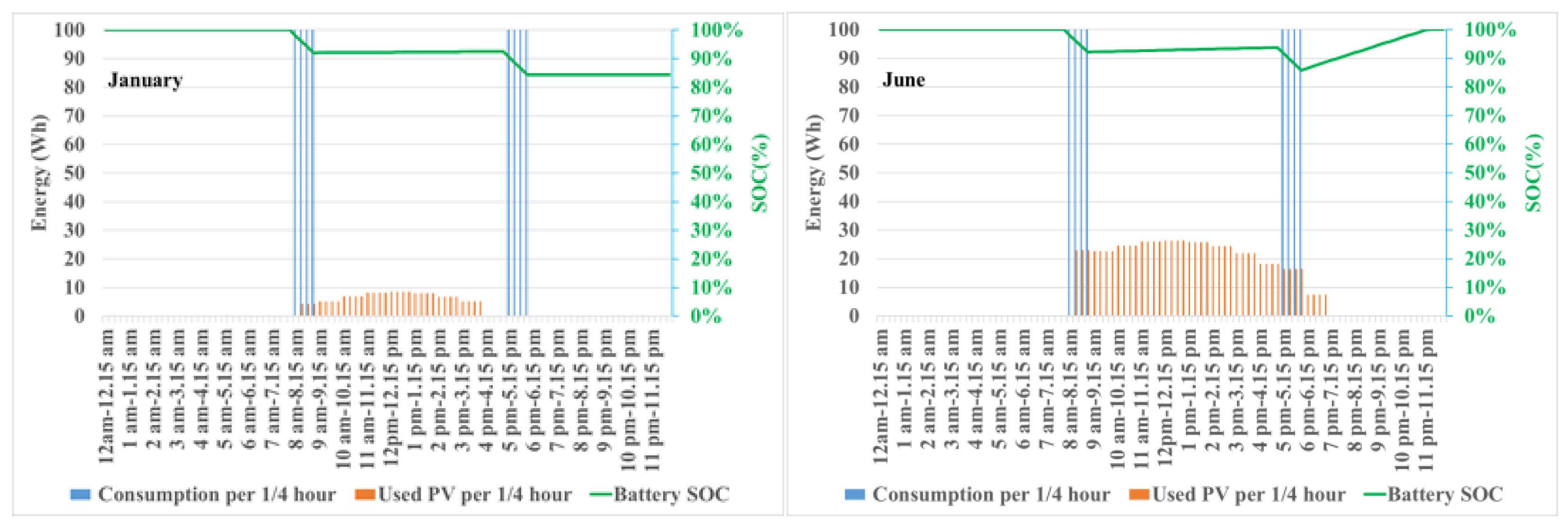
Figure 4.
Yearly PV energy in Malaga and Paris, passenger car, 0.312 kWp solar roof.
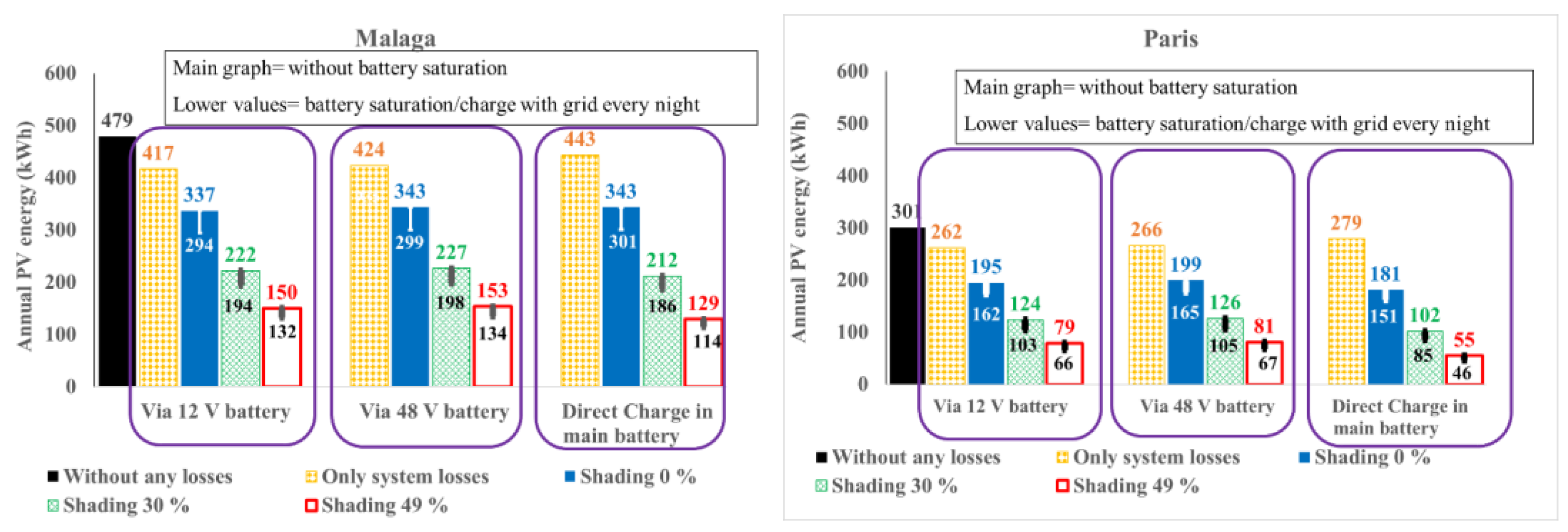
Figure 5.
Yearly PV energy in Malaga and Paris, passenger car, 0.312 kWp solar roof, 50 kWh battery, direct transfer in the main battery, effect of frequency of recharge with the grid.
Figure 5.
Yearly PV energy in Malaga and Paris, passenger car, 0.312 kWp solar roof, 50 kWh battery, direct transfer in the main battery, effect of frequency of recharge with the grid.
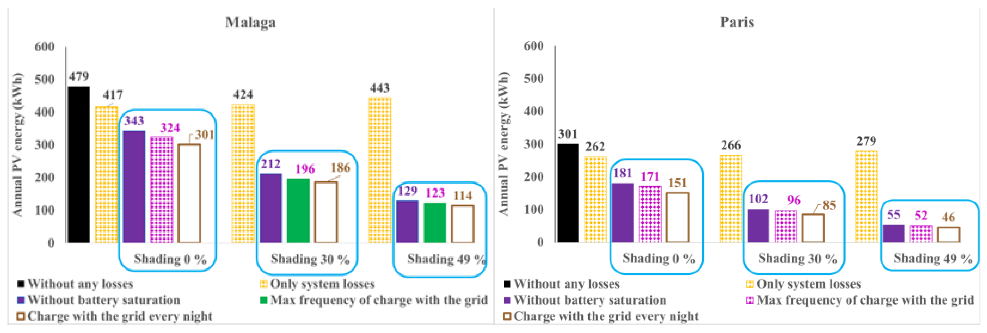
Figure 6.
Yearly distance covered by VIPV in Malaga and Paris, passenger car, 0.312 kWp solar roof and 157 Wh/km electrical consumption.
Figure 6.
Yearly distance covered by VIPV in Malaga and Paris, passenger car, 0.312 kWp solar roof and 157 Wh/km electrical consumption.
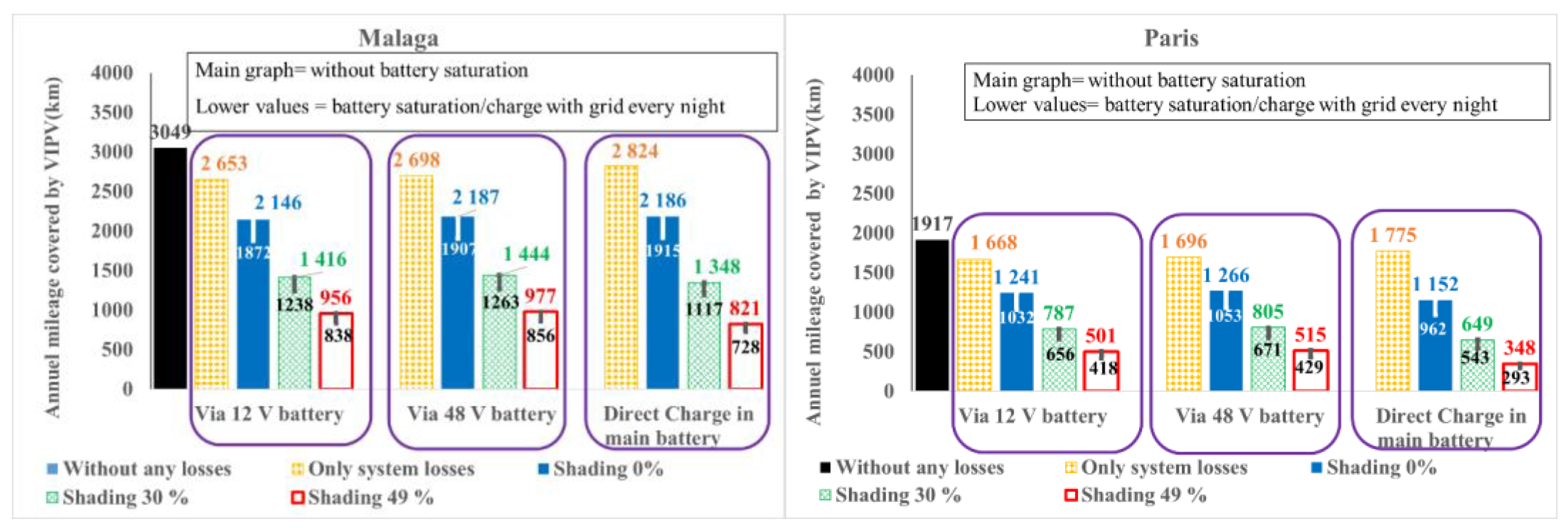
Figure 7.
Yearly distance covered by VIPV in Malaga and Paris, passenger car ,0.312 kWp solar roof, 50 kWh battery, direct charge in HV battery, effect of plugin frequency.
Figure 7.
Yearly distance covered by VIPV in Malaga and Paris, passenger car ,0.312 kWp solar roof, 50 kWh battery, direct charge in HV battery, effect of plugin frequency.
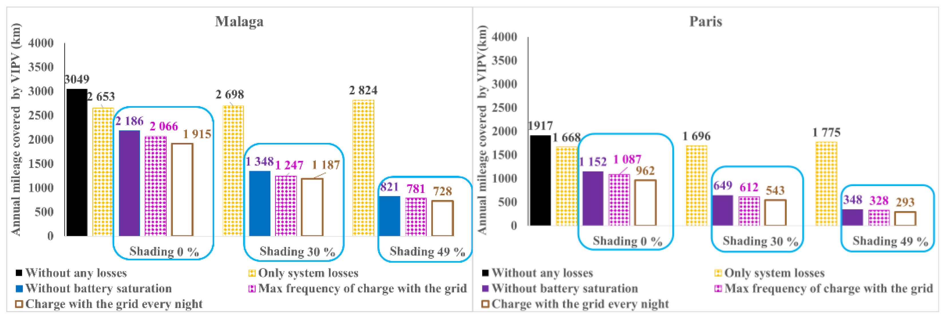
Figure 8.
Average daily distance covered by VIPV, passenger car, 0.312 kWp solar roof and 157 Wh/km electrical consumption with battery saturation/charge every night.
Figure 8.
Average daily distance covered by VIPV, passenger car, 0.312 kWp solar roof and 157 Wh/km electrical consumption with battery saturation/charge every night.
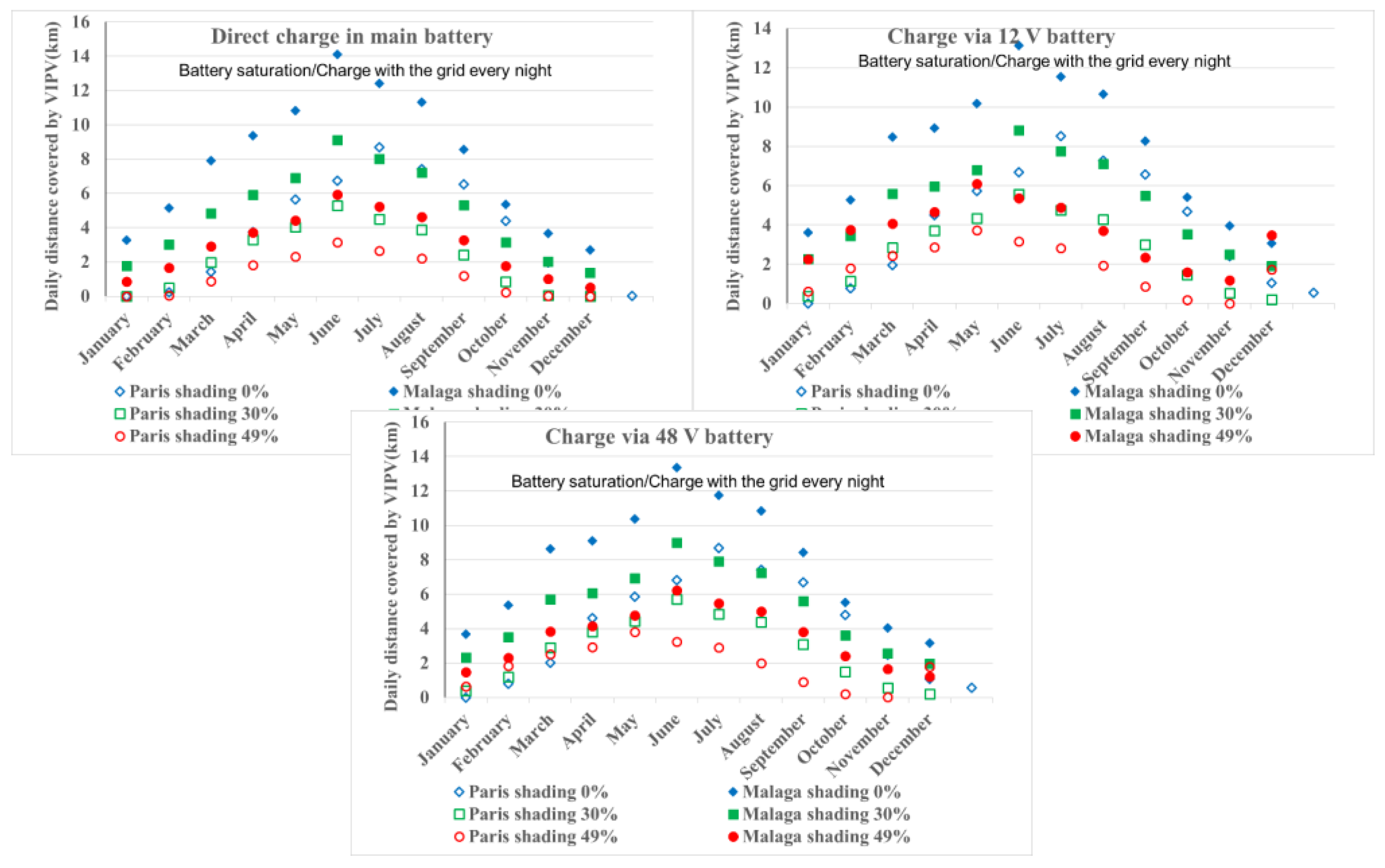
Figure 9.
Explanation of power thresholds effect, schematic application onto a typical sunny day.
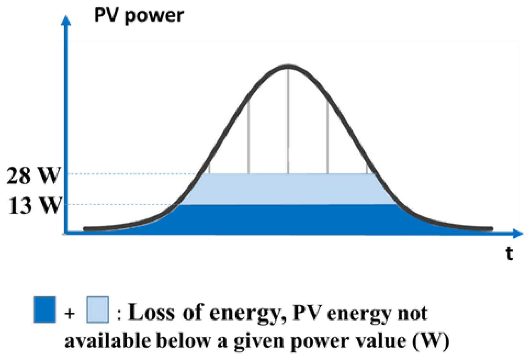
Figure 10.
Yearly distance covered by VIPV in Malaga and Paris, passenger car, 30 % shading, 157 Wh/km electrical consumption, with different peak power and thresholds values.
Figure 10.
Yearly distance covered by VIPV in Malaga and Paris, passenger car, 30 % shading, 157 Wh/km electrical consumption, with different peak power and thresholds values.
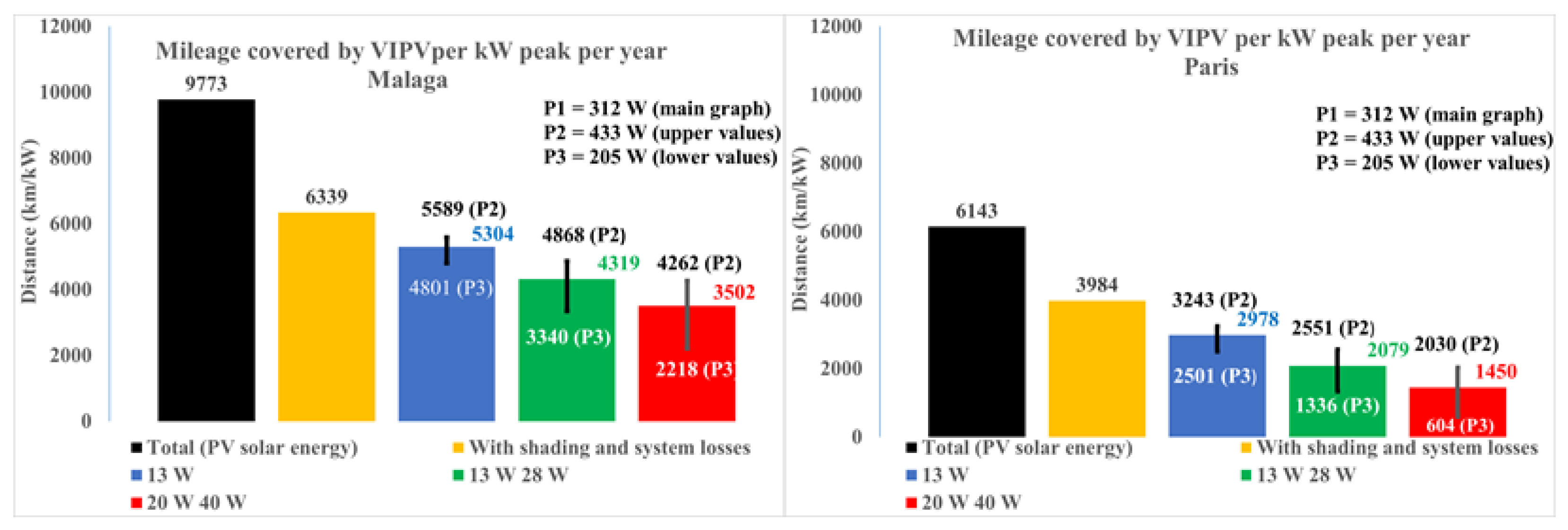
Figure 11.
Avoided emissions in Malaga, 0.312 Wp VIPV, global warming scenario +2.7 °C.
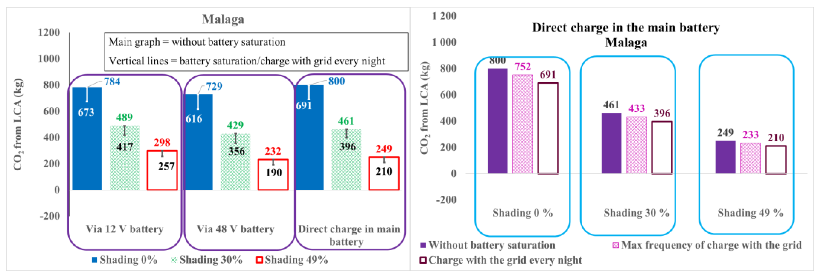
Figure 12.
Avoided emissions in Average Europe, 0.312 Wp VIPV, global warming scenario +2.7 °C.
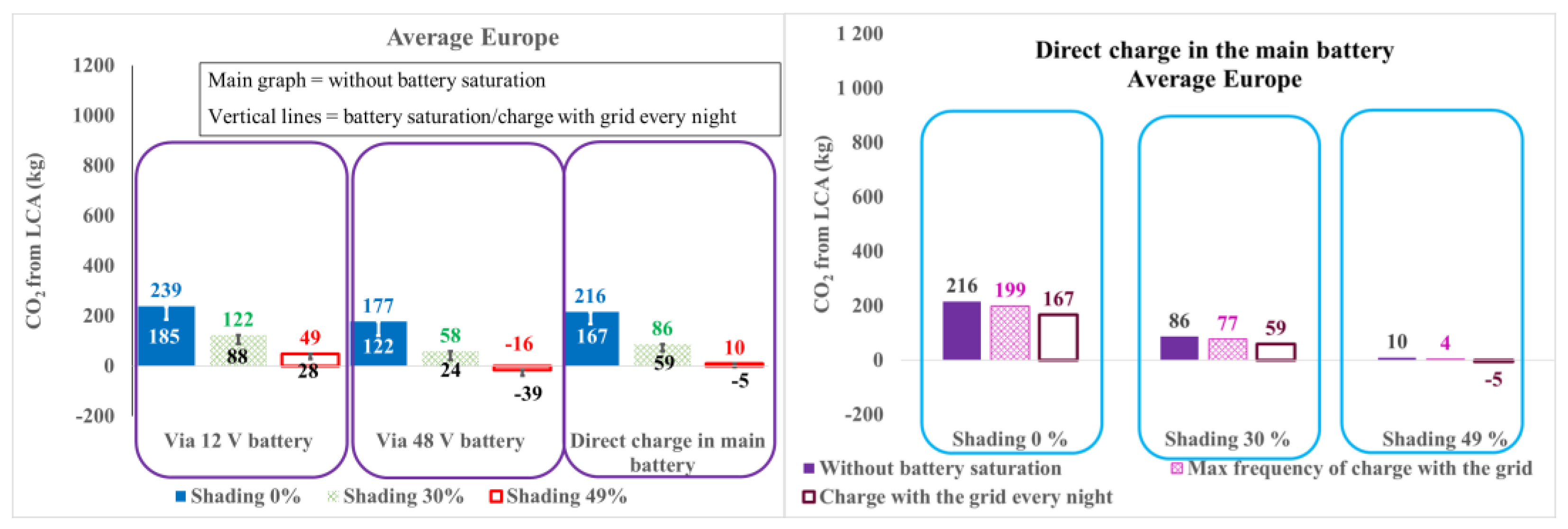
Figure 13.
Avoided emissions in Paris, 0.312 Wp VIPV, global warming scenario +2.7 °C.
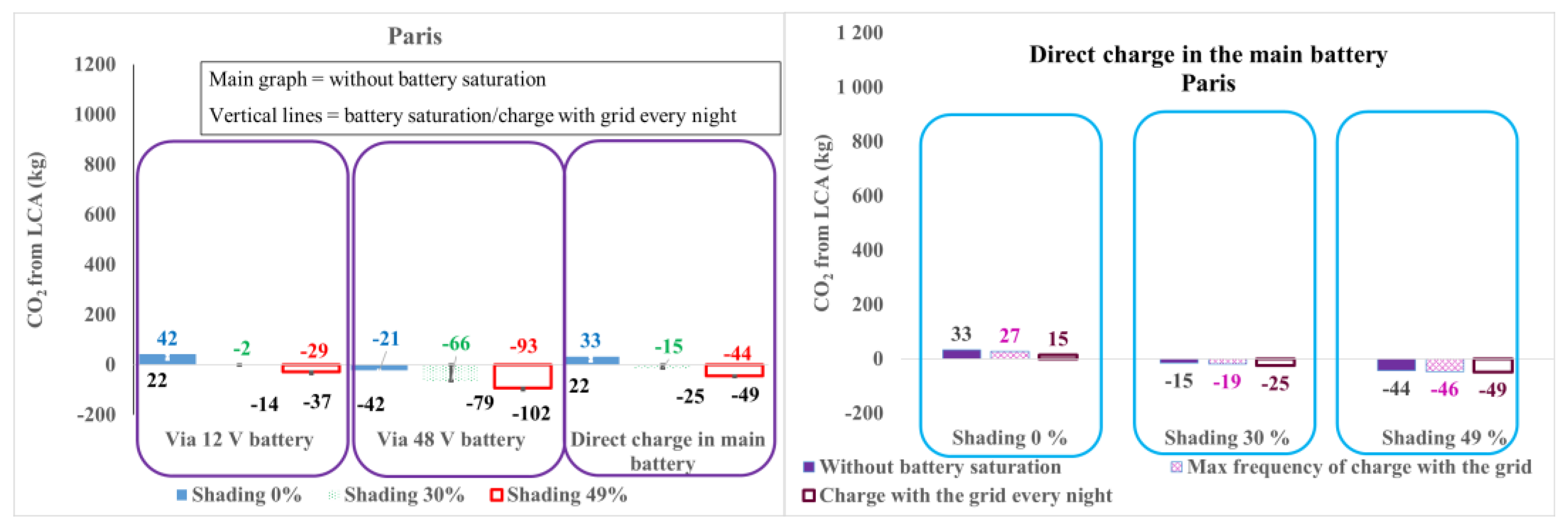
Figure 14.
Yearly distance covered by VIPV in Paris with Lightyear 0 main characteristics 0.981 kWp (Midlife)/1.05 kWp (BOL) solar roof, 109 Wh/km consumption and 60 kWh battery.
Figure 14.
Yearly distance covered by VIPV in Paris with Lightyear 0 main characteristics 0.981 kWp (Midlife)/1.05 kWp (BOL) solar roof, 109 Wh/km consumption and 60 kWh battery.
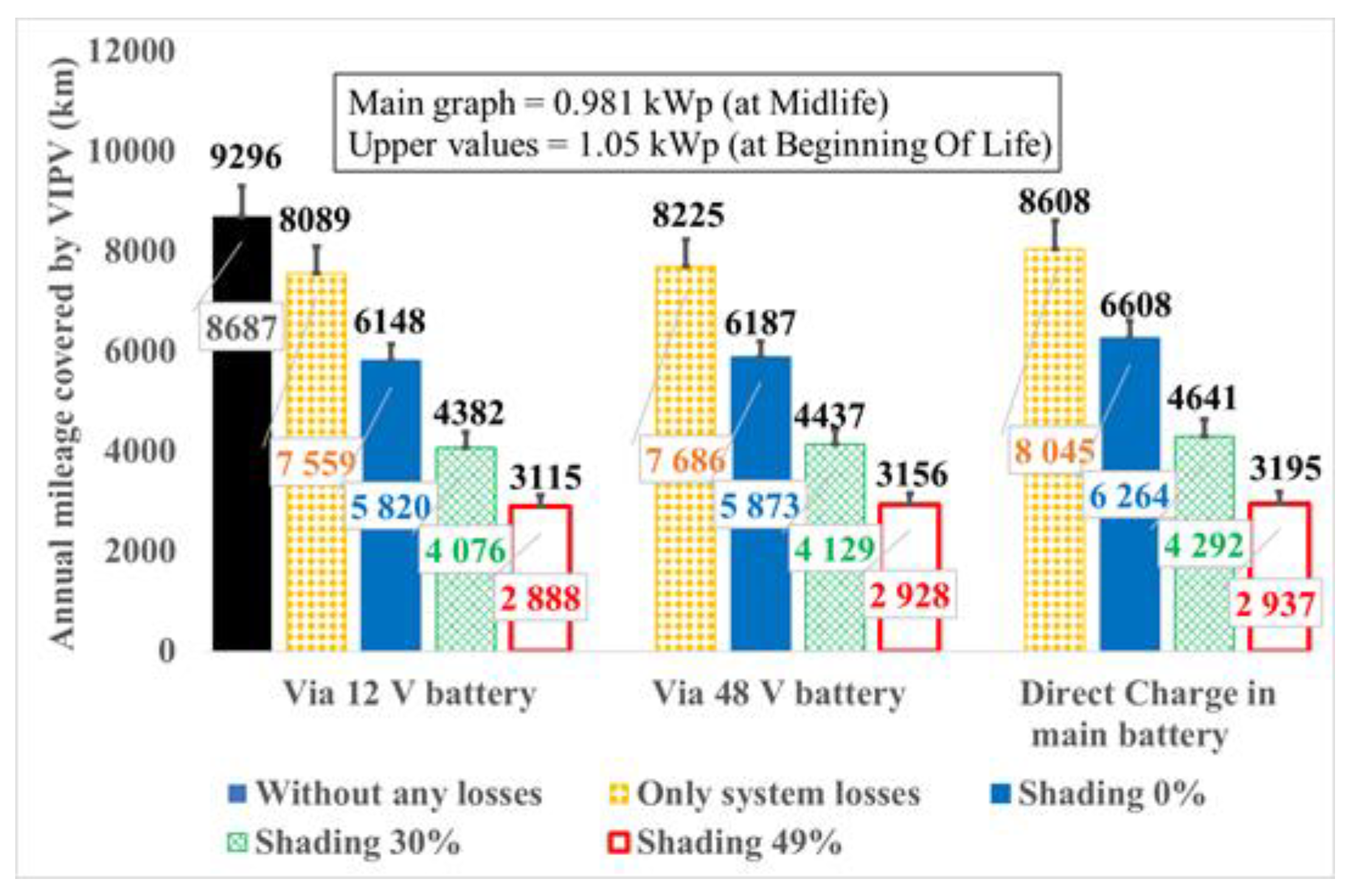

Table 1.
System efficiency for VIPV passenger car (2030 projections) for the three architectures.
| Components | via 12 V battery | via 48 V battery | in main battery |
|---|---|---|---|
| DCDC (PV/LV battery) | 99.1% | 98.7% | NA |
| DCDC (LV/HV) | 95.5% | 97.5% | 97.7% |
| MPPT | 99% | 99% | 99% |
| LV Battery | 97% | 97% | NA |
| DC/AC (battery/engine) | 98.7% | 98.7% | 98.7% |
| HV Battery | 97% | 97% | 97% |
| System Efficiency | 87% | 88.5% | 92.6% |
Table 2.
LCA results (fabrication phase) (kg CO2-eq).
| Component | via 12 V battery | via 48 V battery | in main battery |
|---|---|---|---|
| Total | 76 | 139 | 76 |
| PV module | 62 | 62 | 62 |
| Electronic / cable | 13 | 27 | 13 |
| Additional Battery | NA | 50 | NA |
Table 3.
Variable shading losses between months in Paris.
| January | February | March | April | May | June | July | August | September | October | November | December |
|---|---|---|---|---|---|---|---|---|---|---|---|
| 69 % | 59 % | 29 % | 21 % | 23 % | 25 % | 24 % | 24 % | 23 % | 51 % | 69 % | 64 % |
Table 4.
Simulation results with variable shading between months compared to constant shading of 30 % in Paris.
Table 4.
Simulation results with variable shading between months compared to constant shading of 30 % in Paris.
| Shading losses | Variable between months | 30 % | Evolution | |
|---|---|---|---|---|
| PV useful energy per year (kWh) | Min | 92 | 85 | 8 % |
| Max | 129 | 126 | 2 % | |
| Mileage covered by VIPV per year (km) | Min | 588 | 543 | 8 % |
| Max | 822 | 805 | 2 % | |
| kg CO2-eq | Min | -78 | -79 | 1 |
| Max | 0 | -2 | 2 | |
| Mileage covered by VIPV (km/day) | Min | 0 | 0 | 0 % |
| Max | 6.2 | 5.7 | 9 % |
Table 5.
Simulation results with different shading between driving and parking compared to constant shading of 49 % in Paris and Malaga, energy in kWh.
Table 5.
Simulation results with different shading between driving and parking compared to constant shading of 49 % in Paris and Malaga, energy in kWh.
| Shading losses | 26 % driving/52 %parking | 49% | Evolution | |
|---|---|---|---|---|
| Charge via 12 V battery | Paris | 73 | 74 | -1 % |
| Malaga | 139 | 142 | -2 % | |
| Charge via 48 V battery | Paris | 74 | 76 | -3 % |
| Malaga | 142 | 145 | -2 % | |
| Direct charge in the main battery | Paris | 51 | 52 | -2 % |
| Malaga | 119 | 123 | -3 % |
Table 6.
Influence of lower system efficiency on useful PV energy, 30 % shading; directly charging HV battery and battery never fully charged.
Table 6.
Influence of lower system efficiency on useful PV energy, 30 % shading; directly charging HV battery and battery never fully charged.
| System efficiency | Locality | PV energy (kWh) | Evolution |
|---|---|---|---|
| 93% | Paris | 102 | 0 % |
| Malaga | 212 | 0 % | |
| 80 % | Paris | 77 | -25 % |
| Malaga | 170 | -20 % | |
| 70 % | Paris | 56 | -45 % |
| Malaga | 135 | -36 % |
Table 7.
Comparison of the values for two surfaces of solar roof for passenger car.
| PV surface | 1.44 m² | 2 m² | Evolution | |
|---|---|---|---|---|
| PV peak power (kW) | 0.312 | 0.433 | 39 % | |
| PV useful energy per year (kWh) | Min | 46 | 87 | 47 % |
| Max | 227 | 326 | 30 % | |
| Distance covered by VIPV per year (km) | Min | 293 | 554 | 47 % |
| Max | 1444 | 2078 | 31 % | |
| Distance covered by VIPV | Min | 3.3 | 5.4 | 39 % |
| Best month (km/day) | Max | 14 | 20.9 | 33 % |
Table 8.
Percentage of increase of energy per kWp for a solar vehicle (Lightyear 0 main characteristics) relatively to that of a solarized electric vehicle.
Table 8.
Percentage of increase of energy per kWp for a solar vehicle (Lightyear 0 main characteristics) relatively to that of a solarized electric vehicle.
| Only system losses | Shading 0 % | Shading 30 % | Shading 49 % | |
|---|---|---|---|---|
| Charge via 12 V battery | 0% | 10% | 21% | 35% |
| Charge via 48 V battery | 0% | 9% | 20% | 33% |
| Charge in the main battery | 0% | 27% | 55% | 97% |
Disclaimer/Publisher’s Note: The statements, opinions and data contained in all publications are solely those of the individual author(s) and contributor(s) and not of MDPI and/or the editor(s). MDPI and/or the editor(s) disclaim responsibility for any injury to people or property resulting from any ideas, methods, instructions or products referred to in the content. |
© 2023 by the authors. Licensee MDPI, Basel, Switzerland. This article is an open access article distributed under the terms and conditions of the Creative Commons Attribution (CC BY) license (http://creativecommons.org/licenses/by/4.0/).
Copyright: This open access article is published under a Creative Commons CC BY 4.0 license, which permit the free download, distribution, and reuse, provided that the author and preprint are cited in any reuse.


