
Submitted:
05 June 2023
Posted:
05 June 2023
You are already at the latest version
Abstract
It is common knowledge that estimating the height component of GNSS stations in general is much more problematic than estimating the horizontal position. Many different effects, such as tectonic signals, non-tectonic signals, atmospheric delay, noise, etc., are known to affect the height component of GNSS stations more than the horizontal component. However, the height component of GNSS stations is still poorly estimated. In this study, the height time series of 37 continuous GNSS stations covering the 2014–2019 date range is used from the Turkish National Permanent GNSS Network-Active (TUSAGA-Active). Since it is easier to interpret the effects of the height component due to its topographic features and seasonal changes being more effective than in the rest of the country, stations were chosen in the Eastern Anatolia region of Turkey. The daily coordinates of the GNSS stations were obtained as a result of the GAMIT/GLOBK software solution. By applying time series analysis to the daily coordinate values of the stations, statistically significant trends, periodic and stochastic components of the stations were determined. As a result of the analysis, the vertical velocities of the GNSS stations and the standard deviations of the vertical velocities were determined. Furthermore, when the height components of continuous GNSS stations were examined, it was seen that there were seasonal effects, and it was investigated whether the height components were related to meteorological parameters. For that, simple linear regression analysis was performed to determine how dependent the height components of the continuous GNSS stations were on meteorological parameters. As a result of the analysis, the height components of the continuous GNSS stations are dependent on meteorological parameters such as temperature, pressure, relative humidity, wind speed, and precipitation. In addition, height component time series analysis of continuous GNSS stations was performed by using Autoregressive Moving Average (ARMA) models from linear time series methods. As a result of the study, the performance of the ARMA modeling results again indicated the dependence of the height component of the continuous GNSS stations on the meteorological parameters.
Keywords:
GNSS height component
; GNSS time series
; velocity estimation
; meteorological parameters
; simple linear regression
; autoregressive moving average
1. Introduction
Positioning accuracy with GNSS data analysis in geodesy is 1–2 mm in horizontal coordinates and 5–10 mm in vertical coordinates [1,2,3]. There are two main reasons for the weakness in the vertical component. The first is due to the geometric distribution of satellites in the sky. The latter is due to tropospheric path delay, particularly water vapor [4,5,6,7]. In order to increase the usability of height information obtained in today's highly sensitive geodetic studies, it has become necessary to investigate the disruptive effects on GNSS heights since many error sources first manifest themselves in this component. Increasing the sensitivity of GNSS ellipsoidal heights is possible by developing the most appropriate measurement and evaluation strategies according to the experiment and purpose, taking into account the error sources affecting the heights determined by the GNSS technique. GNSS velocities have improved significantly over the last 20 years due to studies on noise characteristics [8,9], ionospheric effects [10], or multipath and geometry effects [11].
Many GNSS time series analyses can be found in the literature review [12,13,14,15,16,17,18]. The first investigation of the permanent GNSS station time series was done in the 1990s [19,20]. Santamaria-Gomez et al. [17,21] developed different methodologies to estimate vertical velocities in the study. The effect of different antenna calibration models, the effect of different tropospheric delay models, and the geometric distribution of stations in the studied network geometry affect vertical velocities. Also, velocity domains were evaluated by analyzing the type and amplitude of noise content in time series.
A more accurate estimation of the seasonal signal is required to distinguish signals produced only by tectonic movement from other signals. For this reason, Ming et al. [22] performed seasonal signal analysis and long-term trend analysis in height time series at IGS stations. Strong seasonal variations in amplitudes of 4–9 mm were observed in the height component at the IGS stations. In previous studies of GNSS time series, the seasonal signal was thought to have annual or semi-annual periods, which can be described by a harmonic pattern of constant amplitude and phase [12,18,20,23].
Time series analysis employs a variety of techniques to separate tectonic displacement signals from seasonal signals, which are a result of the signal's nature and other factors. Davis et al. [15] proposed a linear Kalman filter model to explain the behavior of a seasonal signal, assuming that the stochastic model includes random noise. However, the hypothesis is implausible since many studies have proven that GNSS time series have flicker noise (FN). In particular, GNSS station velocities are often estimated by assuming the presence of white, flicker, and random walk noise [12,20,24].
Significant semi-annual and annual variations are visible in the height time series created using continuous GNSS station data over several years [25]. Seasonal movement from continuous GNSS observations can be a source of error in the GNSS coordinate time series and needs to be modeled to improve the accuracy of GNSS positioning. One of the important parameters affecting the accuracy of the velocity components at each station is the observation (session) time. The purpose of using different observation times is to increase station location accuracy. In order to minimize seasonal effects, it is recommended to estimate velocities with the help of at least 3 years of observations [26,27].
Wang et al. [28] examined the relationship between climate change and the height component of GNSS stations with the data for July and December from GNSS stations that measure continuously from different networks in Taiwan. As a result of the research, GNSS height values showed that the monthly averages of July values are higher than the interval values, and the difference reaches 2 cm, and it reaches 6 cm in the daily averages.
The main objectives and results of our study are to: first, present a velocity field in the Eastern Anatolia region of Turkey from a continuous GNSS network that has operated for almost 6 years. We obtained realistic uncertainties as well by taking the noise characteristics into account. Also, to improve the accuracy of the height component of the GNSS stations, the effects of seasonal variation are investigated. Since it will not be enough to investigate the effects of seasonal changes alone, it is also intended to increase the accuracy of the height component of GNSS stations with meteorological parameters. For this reason, we used two different approaches to see the effects of meteorological parameters on the vertical component. The first is simple linear regression analysis, and another is the ARMA model.
2. Materials and Methods
2.1. Study Area
The Eastern Anatolia Region is a tectonically active region where many geodetic and geophysical scientific studies have been carried out for many years. A part of these scientific studies is to reveal the current velocity field of the region. In this study, time series analyses were made with the MATLAB program after evaluating the data collected at GNSS stations continuously for about 6 years in the 2014–2019 period with a scientific software, GAMIT/GLOBK. It is aimed to reveal the periodic changes in the GNSS observations with the analyses made and to investigate the effects of these changes in the GNSS studies that have been made before and will be made in the Eastern Anatolia Region. Data from 37 continuous GNSS stations were used (Figure 1). The main subject of the study is to determine the periodic effects as a result of the analysis of the time series of these 37 GNSS stations from which data was collected and to develop strategies to improve the height component of GNSS stations.
In this study, 37 continuous GNSS stations covering the 2014–2019 date range from the Turkey National Permanent GNSS Network-Active (TUSAGA-Active) were used. The stations were chosen from the Eastern Anatolia region of Turkey because it is easier to interpret the effects of the height component due to their topographic features and also because seasonal changes are more effective there than in other parts of the country. By comparing GNSS measurements taken in various months and years, it was possible to investigate the impact of seasonal variation on station location accuracy. The locations of the GNSS stations are given in Figure 1. Eight of the stations used in the application were placed on the terrace; twenty-one of them are on the roof; and three of them are concrete poles. The stations installed on the ground are 2 meters-long concrete pole; the poles installed on the terraces are 3 meters; and the steel poles installed on the roofs are 4 meters. Normally, the stations on the building are expected to be more stationary, but when the time series of the stations are examined, it is seen that this is not the case.
Furthermore, average temperature, pressure, relative humidity, wind speed, and precipitation data from 37 Meteorology General Directorate stations in the study area were used to show the relationship between meteorological parameters and the GNSS height component. In the selection of these stations, attention was paid to ensuring that the data was continuous and in working condition.
2.2. GNSS Time Series in Height Component
Time series analyses are performed for two main purposes: First of all, it is to make predictions for the future by explaining the past with the help of observation values from past periods. The other purpose is to determine the effect of any factor that is effective in the series. This effect can be a momentary event or a set of events spread over a certain period of time. In this way, the degree of impact is determined, and measures are taken or regulations are made for the future. Some changes and irregularities can be seen over the course of the series. These changes and irregularities are caused by the existence of four factors (components) and the difference in the direction and intensity of their effects. These are the trends: seasonal fluctuations, cyclical fluctuations, erratic movements: noise [29,30].
The time series of GNSS stations are obtained as a result of daily processes. Linear, periodic, and irregular movements of reference stations can be determined by time series analysis. The time series of these reference stations can be written for horizontal and vertical components as follows [31,32];
where is the trend component parameter, are amplitude of periodic signals and is the corresponding frequency, is an autoregressive (AR) model parameter, is moving-average (MA) model parameter and is residual (noise) to which we pay more attention.
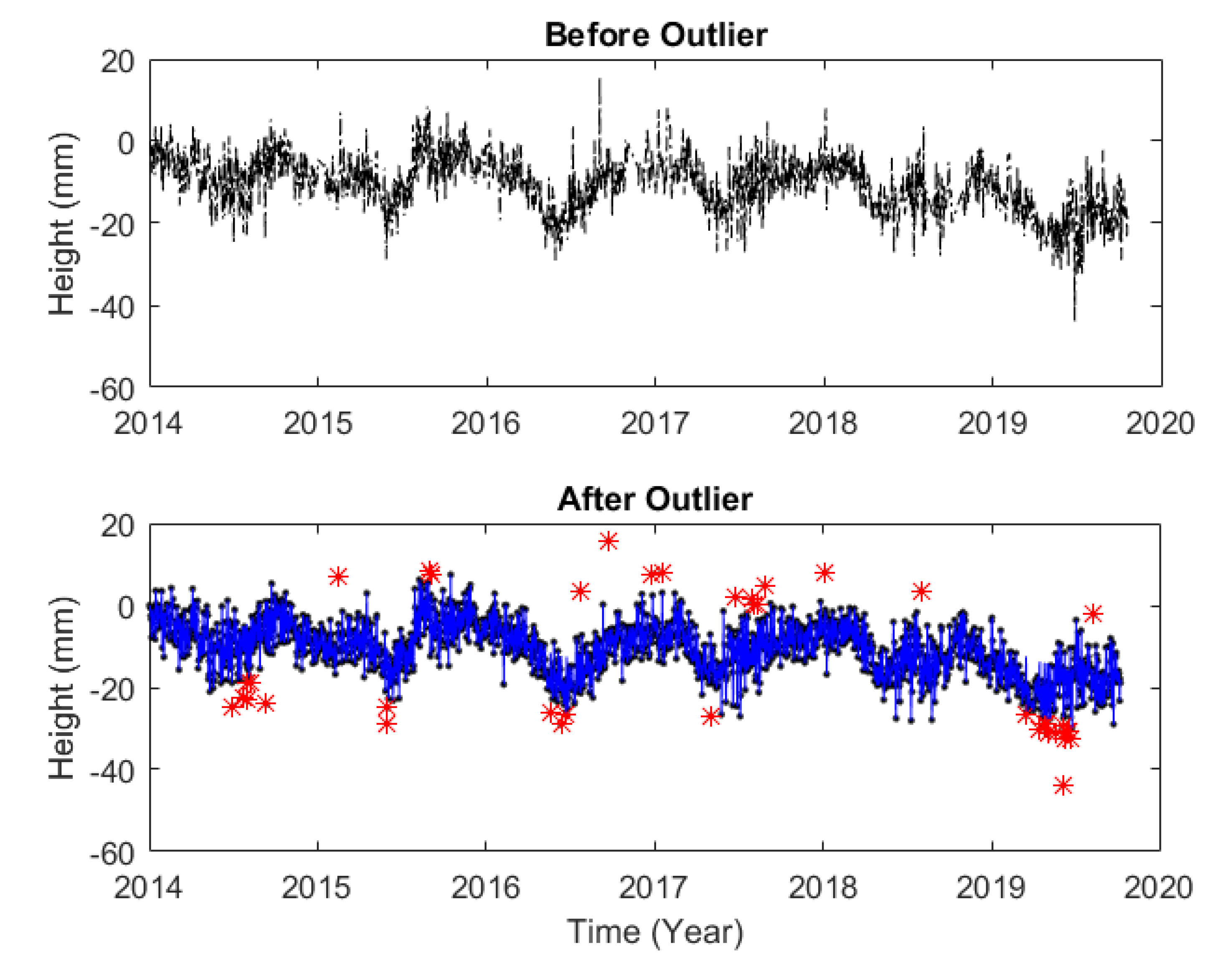
The trend component in the time series represents the time-dependent long-period changes of the series [33]. The Least Squares Method (LSM) separates the trend component from the series in the time series. However, LSM cannot predict the parameters of the time series components in the equation with outliers. The main disadvantage of LSM is its sensitivity to outliers [31].
An outlier is an observation that significantly deviates from other observations in the sample [34]. Prior to the application, the coordinate time series were cleaned for outliers. Outliers should be removed from the time series before starting the analysis. Outliers in the time series were investigated using a robust method. According to the predicted model, outliers were determined and removed from the time series, then gaps in the data were calculated and the time series were reconstructed [35].
Outliers in time series are eliminated from the series by using Bi-square weighted robust predictor methods. New values are determined for the eliminated values in the series. Also, the loss of data can be determined by this method. Bi-square weights minimize a weighted sum of squares, where the weight given to each observation point depends on how far the point is from the fitted line. Points near the line get full weight, whereas points far from the line get reduced weight. Robust fitting with bi-square weights uses an iteratively re-weighted LS algorithm and follows the weight function [35].
Figure 2.
Outlier test for RZE1 station.
Outliers of the stations were removed, the gaps were calculated according to the model, and then the frequencies contained in the series and the period values corresponding to these frequencies were calculated by applying Fast Fourier Transform (FFT) to the height time series where the trend component was removed [36]. Since the peaking values in the graphs differ, the frequency range has been changed according to the suitability of the graphs. Figure 3 shows the power-frequency relationship of GNSS stations of different ellipsoid heights.
In order to better understand and interpret the results obtained, the periods included in each time series were calculated using the equation from the frequencies with high power values in the power-frequency graphs of the stations. Annual periodic movement in the vertical only at SIVS1 and TOK1 stations; semi-annual periodic movement at all stations except ADIY1, ERZ2, and TUF1 stations; seasonal periodic movement at all stations except ARTV, BING, DIV1, FASA, GEME, GUMU, GURU, and TRBN GNSS stations; and much daily periodic motion was observed at all GNSS stations [14,37].
2.3. Simple Linear Regression
The relationship between a single independent variable (x) and the dependent variable (Y) expressed with a linear function is defined as simple linear regression analysis [38].
where the value of is the value of the dependent variable when or in other words, the site where the vertical axis intersects with , while the value of is expressed as the regression coefficient. The difference between the true value of the dependent variable and its predicted value from the model is the error .
In the regression, we try to estimate the independent variable Y by taking the dependent X variables. The results we get as a result of estimation are usually either incomplete or wrong. The real question we have to ask here is how wrong it is. In other words, what we really need to do is find the distance between the actual values and the predicted values. The following are the concepts used to evaluate the regression model [39].
2.3.1. Model Performance
The mean absolute error represents the average of the absolute difference between the actual and predicted values in the dataset. It measures the average of the residuals in the dataset.
(best value = 0; worst value = +∞)
where; predicted value of and means value of .
The mean squared error represents the average of the squared difference between the original and predicted values in the data set. It measures the variance of the residuals.
(best value = 0; worst value = +∞)
The root mean squared error is the square root of mean squared error. It measures the standard deviation of residuals.
(best value = 0; worst value = +∞)
The coefficient of determination or R-squared, represents the proportion of the variance in the dependent variable that is explained by the linear regression model. It is a scale-free score, irrespective of the values being small or large, the value of R square will be less than one.
(worst value = −∞; best value = +1)
Both RMSE and R-squared quantify how well a linear regression model fits a dataset. The RMSE tells how well a regression model can predict the value of a response variable in absolute terms, while R-squared tells how well the predictor variables can explain the variation in the response variable [40].
2.4. The Autoregressive Moving-Average (ARMA)
models are used for modeling stationary data and are a combination of and models. In these models, the observation value of any period of a time series is expressed as a linear combination of a certain number of previous observation values and the error term. If the model is a combination of and model, it contains terms and is expressed as [41].
Here, is known as normal white noise process. It has a zero mean and variance . is the amount of data in the time series [42]. parameters should satisfy the condition for stationarity and parameters should satisfy the conditions for inevitability [43].
ARMA model was applied to the height component of GNSS stations in the same region by using the daily average temperature, pressure, relative humidity, wind speed, and precipitation values measured at 37 meteorology stations in the study area. Model results for four GNSS stations are given in Figure 4 as an example, and the model results for all stations subject to the study are given in Table 1.
ARMA model results are generally consistent with the time series of all stations. The RMS values are generally less than 5 mm in the vertical directions, except for ARTV, ERZ2, GIRS, MUUS, and SIRT1 stations. The RMS values of the vertical component were computed with all meteorological data.
3. Results and Discussion
3.1. Seasonal Variation
In this study, the effects of seasonal variation on the vertical position accuracy of GNSS calculated by time series analysis of continuous GNSS stations were investigated. Weather changes and water vapor in the atmosphere affect the position accuracy of GNSS and cause fluctuations in GNSS height values. It is also known that the height component has more air passage changes. By applying time series analysis to the daily coordinate values of the stations, statistically significant trends, periodic, and stochastic components of the stations were determined. As a result of the analysis, the vertical annual velocities of the stations and the standard deviations of the velocities were determined.
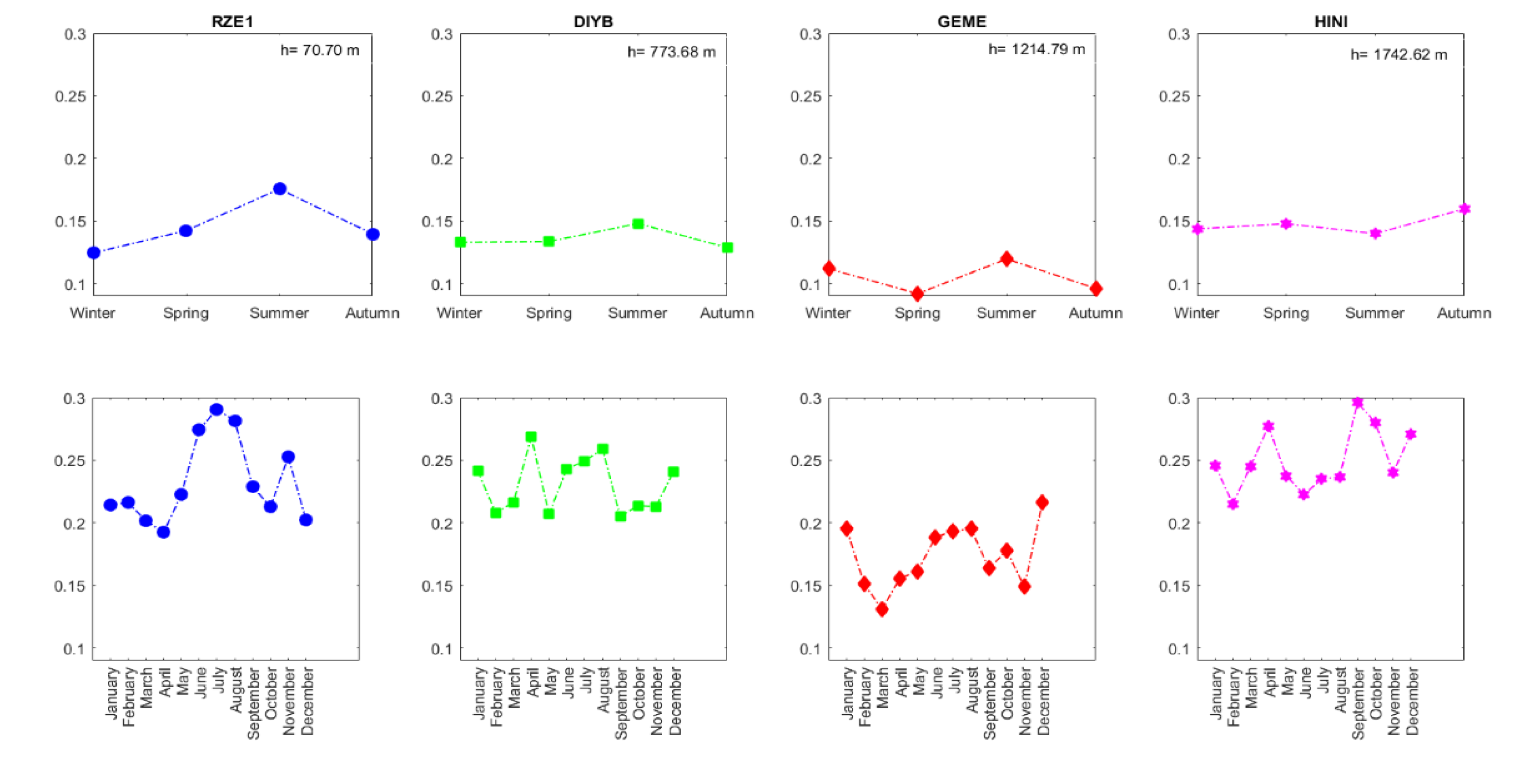
For the stations determined according to the ellipsoid heights, the velocity and standard deviation values of the height component were calculated for each month, season, and year. As the ellipsoid height increases, the velocity and its standard deviation values decrease. While the minimum vertical velocity values are observed for the station with the lowest ellipsoidal height in winter, for the station with the highest ellipsoidal height in autumn, the minimum standard deviation values are determined in winter for the station with the lowest ellipsoidal height, and in summer for the station with the highest ellipsoidal height. According to the results obtained, the coordinate displacements caused by seasonal variation may be important, and their effects should be considered, especially in high-precision geodetic surveys [44].
Figure 6.
Vertical velocity variations of GNSS stations (The minimum velocity for RZE1 station in winter (December), for DIYB station in winter (December), for GEME station in summer (August), and for HINI station in autumn (November). The maximum velocity for RZE1 station in autumn (September), for DIYB station in autumn (October), for GEME station in spring (April), and for HINI station in winter (December)).
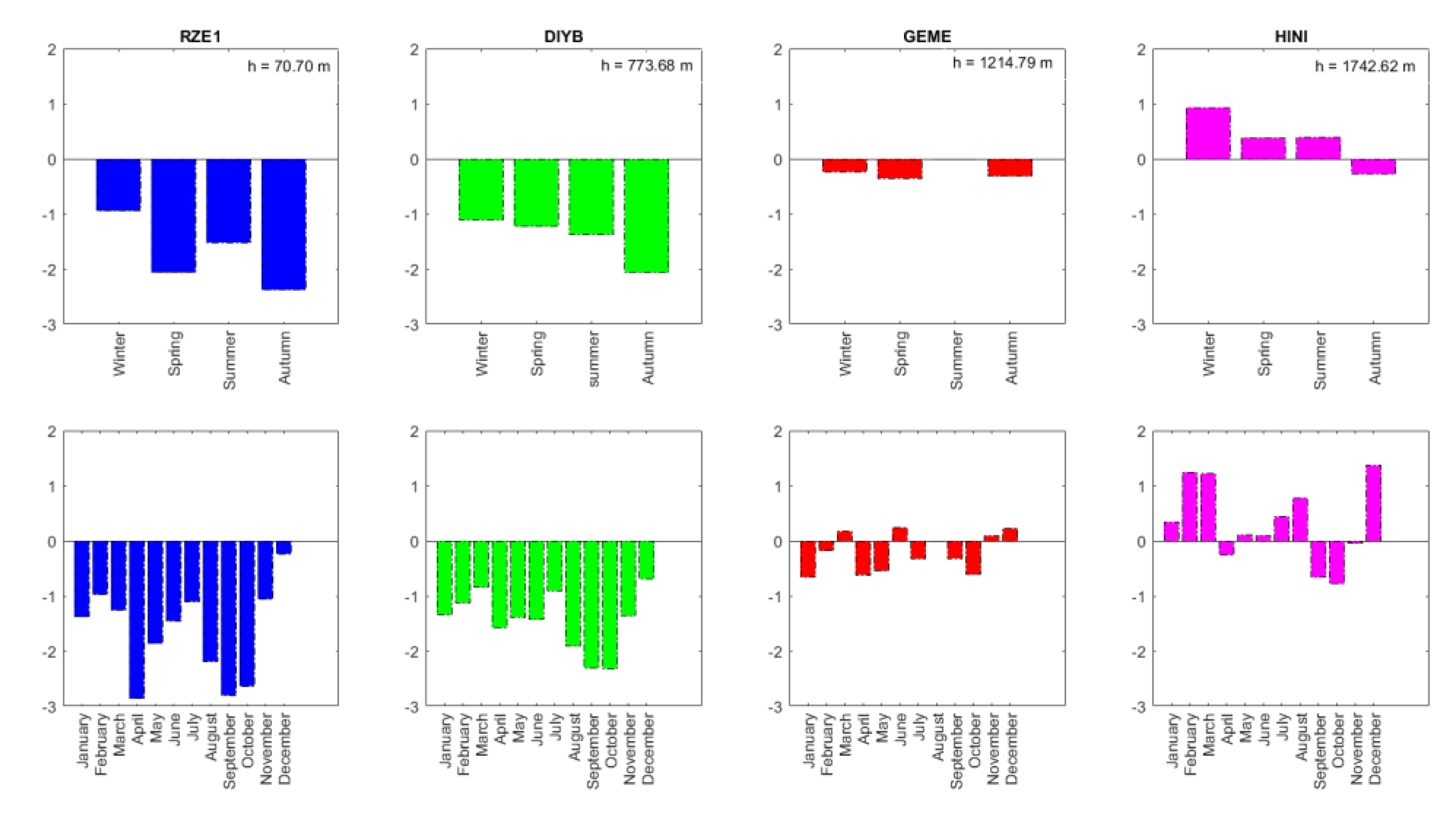
Figure 7.
Standard deviation variations for vertical velocities of GNSS stations (The minimum standard deviation for RZE1 GNSS station in winter (December), for DIYB GNSS station in winter (February), for GEME GNSS station in spring (March), and for HINI GNSS station in summer (June). The maximum standard deviation for RZE1 GNSS station in summer (July), for DIYB GNSS station in summer (August), for GEME GNSS station in summer (August), and for HINI GNSS station in autumn (September)).
In addition, the velocity values of the stations were calculated for different years, and a decrease was observed in the height component depending on the observation duration. As the observation duration for the height component increases, both the velocity values and their standard deviation values decrease. In order to avoid velocity estimation errors completely, the data length should be more than 4.5 years.
It has been determined that the height components of the GNSS stations used in the application make periodic movements. Considering that this may be due to seasonal effects, daily average temperature, pressure, relative humidity, wind speed, and precipitation values between 2014 and 2019 of meteorological stations in the cities where the GNSS stations are located were obtained from the General Directorate of Meteorology. By using these parameters, the relationship of the stations with the height component was investigated.

Table 2.
Regression results for GNSS stations of different ellipsoidal heights (m).
| temperature | R-squared | Standard error | MAE | MSE | RMSE | Height | |
| RZE1 | 0.781 | 0.012 | 0.0880 | 0.01 | 0.1135 | 70.69 | |
| DIYB | 0.864 | 0.009 | 0.0943 | 0.01 | 0.1173 | 773.67 | |
| GEME | 0.850 | 0.008 | 0.1072 | 0.02 | 0.1371 | 1214.79 | |
| HINI | 0.839 | 0.008 | 0.1006 | 0.02 | 0.1302 | 1742.62 | |
| pressure | R-squared | Standard error | MAE | MSE | RMSE | Height | |
| RZE1 | 0.845 | 0.019 | 0.1106 | 0.02 | 0.1311 | 70.69 | |
| DIYB | 0.801 | 0.014 | 0.0987 | 0.02 | 0.1250 | 773.67 | |
| GEME | 0.894 | 0.009 | 0.1122 | 0.02 | 0.1458 | 1214.79 | |
| HINI | 0.864 | 0.008 | 0.1004 | 0.02 | 0.1288 | 1742.62 | |
| relative humidity | R-squared | Standard error | MAE | MSE | RMSE | Height | |
| RZE1 | 0.843 | 0.019 | 0.1087 | 0.02 | 0.1136 | 70.69 | |
| DIYB | 0.797 | 0.014 | 0.0946 | 0.01 | 0.1184 | 773.67 | |
| GEME | 0.894 | 0.009 | 0.1021 | 0.02 | 0.1338 | 1214.79 | |
| HINI | 0.861 | 0.008 | 0.0986 | 0.02 | 0.1248 | 1742.62 | |
| wind speed | R-squared | Standard error | MAE | MSE | RMSE | Height | |
| RZE1 | 0.845 | 0.019 | 0.1029 | 0.02 | 0.1267 | 70.69 | |
| DIYB | 0.794 | 0.014 | 0.0968 | 0.01 | 0.1223 | 773.67 | |
| GEME | 0.893 | 0.009 | 0.1096 | 0.02 | 0.1404 | 1214.79 | |
| HINI | 0.861 | 0.008 | 0.0967 | 0.02 | 0.1225 | 1742.62 | |
| precipitation | R-squared | Standard error | MAE | MSE | RMSE | Height | |
| RZE1 | 0.847 | 0.019 | 0.1122 | 0.02 | 0.1371 | 70.69 | |
| DIYB | 0.796 | 0.014 | 0.0962 | 0.01 | 0.1212 | 773.67 | |
| GEME | 0.895 | 0.009 | 0.1095 | 0.02 | 0.1396 | 1214.79 | |
| HINI | 0.858 | 0.008 | 0.0952 | 0.01 | 0.1201 | 1742.62 |
The estimation of the parameters was carried out with the least squares method. Hypothesis tests determined the suitability of the regression model and the significance of the regression coefficients.
3.2. Determination of Noise Patterns
Noise analysis is needed to reveal the characteristics of the stations and to investigate the time series more deeply. [12,13,20,24,29] emphasized that GNSS time series contain time-independent white noise (WN), time-dependent flicker noise (FN), and random walk noise (RWN). In all these analyses, it was observed that the vertical component had more noise than the horizontal component, and the periodic motion of the vertical component was more pronounced.
The most suitable noise model for the height component of the stations was examined with the CATS software [45]. CATS is software that uses Maximum Likelihood Estimation (MLE) to fit a multi-parameter model to time series such as fixed GNSS station coordinates. Using MLE, it is possible to estimate the amplitudes of multiple noises and the unknown (e.g., velocity, periodic signals, and coordinate pulses) simultaneously [12,36].
Three noise types and combinations of these noise types were used in the study carried out to reveal the correlated noise models. First, the noise was assumed to be only WN, then a combination of WN+FN and WN+RWN was used. The preferred noise pattern was determined to be one of these three combinations. In the second stage, the amplitudes and spectral indices of the noise model were presented simultaneously with the WN.
As a result of the analysis made, the most appropriate noise model for the height component is given in Table 3. When the MLE values are examined, it is seen that the WN+FN model is the most dominant model among the three noise models, as suggested by [12,20,24]. Again, for all stations, the WN+FN noise model was found to be more suitable than the WN+RWN noise model [46]. In addition, when the results are examined, the values of WN+FN and WN+RWN noise combinations for all stations are quite close to each other.
Amplitudes are one of the important parameters for noise analysis. The amplitudes indicate the magnitude of the appropriate noise pattern present in the available data. The calculated amplitudes for the noise models are given in Figure 8. It is seen that the lowest noise amplitudes are for WN. It is considered that the reason for the WN amplitude differences is the use of different GNSS receivers at the stations. A significant amount of WN amplitudes and seasonal atmospheric mass distributions are considered to reflect more general physical-based processes, such as atmospheric noise. A very small amount of RWN amplitude also results from more regional-scale processes such as atmospheric effects [12,25,47].
As a result of the analysis, the velocities for the height component of the stations were obtained. When the annual velocity of the height coordinate components of the stations is examined, a vertical velocity value in the (+) direction was observed at ADIY, ADIY1, EKIZ, ERGN, ERZR, and HINI GNSS stations; that is, the height value increased. While the highest vertical velocity value was seen at station ADIY1 with a value of 4.92 mm/year, the smallest vertical velocity value was obtained at station ERZR with a value of 0.03 mm/year. At other stations, a vertical velocity value in the (-) direction was observed, that is, the height value decreased. The smallest vertical velocity value was -0.03 mm/year at SIRT GNSS station, and the vertical velocity was -7.10 mm/year at UDE1 GNSS station. The vertical velocities of GNSS stations are given in Figure 9.
4. Conclusions
The goal of this paper is to find a way to increase the accuracy of the height component of continuous observation GNSS stations. For the vertical displacement analysis of the region, we selected 37 GNSS stations and processed approximately 6 years of continuous data.
First of all, data arrangements were made, and an outlier test was used in MATLAB ver. R2015b (The MathWorks, Inc., USA). After data editing was completed, time series were plotted, and anomalies were investigated. The seasonal behavior of GNSS stations was examined, and strong seasonal and interannual signals were found at all stations. It is also clearly seen that GNSS signals have a lot of noise. CATS software is used for spectral analysis. As expected, the most appropriate noise model for the station was found to be the WN+FN noise model. Then, the relationship between seasonal variation and vertical time series was examined. As a result of the analysis, the vertical seasonal and annual velocities of the stations and the standard deviations of the velocities were determined. The results are variable for stations with different ellipsoid heights. However, as expected, as the observation time increased, the velocity and standard deviation values improved. Furthermore, when the height components of continuous GNSS stations were examined, it was seen that there were seasonal effects, and it was investigated whether the height components were related to meteorological parameters. Simple linear regression analysis was performed to determine how dependent the height components of the continuous GNSS stations were on meteorological parameters. As a result of the analysis, the height components of the continuous GNSS stations are dependent on meteorological parameters such as temperature, pressure, relative humidity, wind speed, and precipitation. In addition, height component time series analysis of continuous GNSS stations was performed by using Autoregressive Moving Average (ARMA) models from linear time series methods. As a result of the study, the performance of the ARMA modeling results again indicated the dependence of the height component of the continuous GNSS stations on the meteorological parameters.
The consideration of the above-mentioned analysis may improve the quality of the station coordinate estimates, especially for the up component.
Author Contributions
Conceptualization, N.T.U. and U.D.; methodology, N.T.U. and U.D.; software, N.T.U.; investigation, N.T.U.; resources, N.T.U.; writing—original draft preparation, N.T.U.; writing—review and editing, N.T.U. and U.D.; visualization, N.T.U. All authors have read and agreed to the published version of the manuscript.
Funding
This research received no external funding.
Acknowledgments
In this paper, the figures with geographical maps were generated with the Generic Mapping Tools (GMT) [48]. and all the other figures and code were generated with MATLAB and Python. The authors are grateful to the organizations that provided the data: General Directorate of Mapping (HGM) for TUSAGA-Active data; Seda Özarpacı for processing GNSS data; Meteorology General Directorate for meteorological data; and Simon D. P. Williams for providing Create and Analysis Time Series (CATS) software [45].
Conflicts of Interest
The authors declare no conflict of interest.
Appendix A
See Table 4.
Table 4.
Vertical velocity field .
| Station | Start | End | TotalData | ExistingData | MissingData (%) | ||||
|---|---|---|---|---|---|---|---|---|---|
| ADIY | 38,22 | 37,74 | 1.01.2014 | 26.12.2016 | 1091 | 739 | 32,26 | 0.28 | 0.23 |
| ADIY1 | 38,26 | 37,76 | 1.12.2018 | 20.10.2019 | 324 | 319 | 1,54 | 4.92 | 1.06 |
| ARPK | 38,48 | 39,04 | 1.01.2014 | 20.10.2019 | 2118 | 1926 | 9,07 | -2.24 | 0.10 |
| ARTV | 41,81 | 41,17 | 1.01.2014 | 20.10.2019 | 2118 | 1876 | 11,43 | -2.52 | 0.10 |
| BAYB | 40,19 | 40,25 | 1.01.2014 | 20.10.2019 | 2118 | 1909 | 9,87 | -0.66 | 0.07 |
| BING | 40,50 | 38,88 | 1.01.2014 | 20.10.2019 | 2118 | 1933 | 8,73 | -1.01 | 0.10 |
| BTMN | 41,15 | 37,86 | 1.01.2014 | 20.10.2019 | 2118 | 1710 | 19,26 | 1.93 | 0.09 |
| DIV1 | 38,11 | 39,37 | 1.10.2017 | 20.10.2019 | 750 | 654 | 12,80 | -5.45 | 0.32 |
| DIYB | 40,18 | 37,95 | 1.01.2014 | 20.10.2019 | 2118 | 1871 | 11,66 | -1.39 | 0.07 |
| EKIZ | 37,18 | 38,05 | 1.01.2014 | 20.10.2019 | 2118 | 1882 | 11,14 | 0.08 | 0.08 |
| ELAZ | 39,25 | 38,64 | 1.01.2014 | 20.10.2019 | 2118 | 1961 | 7,41 | -3.54 | 0.10 |
| ERGN | 39,75 | 38,26 | 1.01.2014 | 20.10.2019 | 2118 | 1896 | 10,48 | 0.26 | 0.09 |
| ERZ2 | 39,69 | 39,70 | 1.01.2017 | 20.10.2019 | 1023 | 921 | 9,97 | -5.50 | 0.36 |
| ERZR | 41,25 | 39,90 | 1.01.2014 | 20.10.2019 | 2118 | 1622 | 23,42 | 0.03 | 0.08 |
| FASA | 37,48 | 41,04 | 1.01.2014 | 20.10.2019 | 2118 | 1570 | 25,87 | -0.86 | 0.07 |
| GEME | 36,08 | 39,18 | 1.01.2014 | 20.10.2019 | 2118 | 1578 | 25,50 | -0.22 | 0.06 |
| GIRS | 38,38 | 40,92 | 1.01.2014 | 20.10.2019 | 2118 | 1749 | 17,42 | -0.67 | 0.09 |
| GUMU | 39,51 | 40,43 | 1.01.2014 | 20.10.2019 | 2118 | 1892 | 10,67 | -0.05 | 0.08 |
| GURU | 37,30 | 38,71 | 1.01.2014 | 20.10.2019 | 2118 | 1912 | 9,73 | -1.01 | 0.07 |
| HINI | 41,69 | 39,36 | 2.01.2014 | 20.10.2019 | 2118 | 1652 | 22,00 | 0.45 | 0.07 |
| HORS | 42,16 | 40,04 | 1.01.2014 | 20.10.2019 | 2118 | 1567 | 26,02 | -1.63 | 0.09 |
| MALY | 38,21 | 38,33 | 1.01.2014 | 20.10.2019 | 2118 | 1615 | 23,75 | -1.17 | 0.08 |
| MAR1 | 36,86 | 37,59 | 1.07.2017 | 20.10.2019 | 1023 | 897 | 14,50 | -2.32 | 0.29 |
| MUUS | 41,50 | 38,79 | 3.01.2014 | 20.10.2019 | 2116 | 1622 | 23,35 | -1.58 | 0.14 |
| RDIY | 37,33 | 40,38 | 1.01.2014 | 20.10.2019 | 2118 | 1848 | 12,75 | -1.14 | 0.08 |
| RHIY | 38,77 | 39,90 | 1.01.2014 | 20.10.2019 | 2118 | 1902 | 10,20 | -0.33 | 0.08 |
| RZE1 | 40,49 | 41,03 | 1.01.2014 | 20.10.2019 | 2118 | 1920 | 9,35 | -1.74 | 0.08 |
| SAM1 | 36,33 | 41,30 | 1.01.2014 | 20.10.2019 | 2118 | 1942 | 8,31 | -0.59 | 0.10 |
| SIRT | 41,93 | 37,93 | 1.01.2014 | 19.10.2019 | 2118 | 1871 | 11,66 | -0.03 | 0.11 |
| SIV1 | 39,32 | 37,75 | 1.07.2017 | 20.10.2019 | 841 | 730 | 13,20 | -6.13 | 0.35 |
| SIVS | 37,00 | 39,74 | 1.01.2014 | 20.10.2019 | 2118 | 1857 | 13,32 | -0.32 | 0.07 |
| SSE1 | 38,10 | 40,16 | 1.10.2017 | 20.10.2019 | 750 | 645 | 14,00 | -3.76 | 0.38 |
| TNCE | 39,54 | 39,10 | 29.03.2014 | 20.10.2019 | 2031 | 1824 | 10,19 | -1.55 | 0.09 |
| TOK1 | 36,55 | 40,33 | 1.01.2014 | 20.10.2019 | 2118 | 1894 | 10,58 | -0.88 | 0.08 |
| TRBN | 39,71 | 41,00 | 21.01.2014 | 20.10.2019 | 2098 | 1834 | 12,58 | -0.701 | 0.09 |
| TUF1 | 36,20 | 38,26 | 1.01.2014 | 20.10.2019 | 2118 | 1922 | 9,25 | -0.38 | 0.08 |
| UDE1 | 41,54 | 40,52 | 1.10.2017 | 20.10.2019 | 750 | 590 | 21,33 | -7.10 | 0.36 |
References
- Bock, O.; Doerflinger, E. Atmospheric processing methods for high accuracy positioning with the Global Positioning System. in Proc. COST Action 716 Workshop, 2000.
- Johasson, J.; Emardson, T.; Jarlemark, P.; Gradinarsky, L.; Elgered, G. The atmospheric influence on the results from the Swedish GPS network. Phys. Chem. Earth 1998, 23, 107–112. [Google Scholar] [CrossRef]
- Liou, Y.-A.; Huang, C.-Y. Teng, Y-T. Precipitable water observed by ground-based GPS receivers and microwave radiometry. Earth Space Sci. 2000, 52, 445–450. [Google Scholar]
- Davis, J.; Herring, T.; Shapiro, I.; Rogers, A. Elgered, G. Geodesy by radio interferometry: Effects of atmospheric modeling errors on estimates of baseline length. Radio Sci. 1985, 20, 1593–1607. [Google Scholar]
- Dodson, A.; Shardlow, P.; Hubbard, L.; Elgered, G. Jarlemark, P. Wet tropospheric effects on precise relative GPS height determination. J. Geod. 1996, 70, 188–202. [Google Scholar]
- Emardson, T.R.; Jarlemark, P.O. Atmospheric modelling in GPS analysis and its effect on the estimated geodetic parameters. J. Geod. 1999, 73, 322–331. [Google Scholar] [CrossRef]
- Liou, Y.-A.; Teng, Y.-T.; Van Hove, T.; Liljegren, J.C. Comparison of precipitable water observations in the near tropics by GPS, microwave radiometer, and radiosondes. J. Appl. Meteorol. 2001, 40, 5–15. [Google Scholar] [CrossRef]
- Williams, S.D.P. Offsets in Global Positioning System time series. J. Geophys. Res. Solid Earth 2003, 108. [Google Scholar] [CrossRef]
- Williams, S.D.P. The effect of coloured noise on the uncertainties of rates estimated from geodetic time series. Journal of Geod. 2003, 76, 483–494. [Google Scholar] [CrossRef]
- Petrie, E.J.; King, M.A.; Moore, P.; Lavallee, D.A. Higher-order ionospheric effects on the GPS reference frame and velocities. J. Geophys. Res. Solid Earth 2010, 115. [Google Scholar] [CrossRef]
- King, M.A.; Watson, C.S. Long GPS coordinate time series: Multipath and geometry effects. J. Geophys. Res. Solid Earth 2010, 115. [Google Scholar] [CrossRef]
- Williams, S.D.P.; Bock, Y.; Fang, P.; Jamason, P.; Nikolaidis, R.M.; Prawirodirdjo, L.; Miller, M.; Johnson, D. J. Error analysis of continuous GPS position time series. J. Geophys. Res. Solid Earth 2004, 109. [Google Scholar] [CrossRef]
- Amiri-Simkooei, A.R.; Tiberius, C.C.J.M.; Teunissen, P.J.G. Assessment of noise in GPS coordinate time series: Methodology and results. J. Geophys. Res. Solid Earth 2007, 112. [Google Scholar] [CrossRef]
- Bogusz, J.; Klos, A. On the significance of periodic signals in noise analysis of GPS station coordinates time series. GPS Solut. 2016, 20, 655–664. [Google Scholar] [CrossRef]
- Davis, J.L.; Wernicke, B.P.; Tamisiea, M.E. On seasonal signals in geodetic time series. J. Geophys. Res. Solid Earth 2012, 117. [Google Scholar] [CrossRef]
- Masson, C.; Mazzotti, S.; Vernant, P. Precision of continuous GPS velocities from statistical analysis of synthetic time series. Solid Earth 2019, 10, 329–342. [Google Scholar] [CrossRef]
- Santamaria-Gomez, A. , Estimation of crustal vertical movements with GPS in a geocentric frame, within the framework of the TIGA project. Doctoral School of Astronomy and Astrophysics Of Île-De-France, 2010.
- Langbein, J. Noise in GPS displacement measurements from Southern California and Southern Nevada. J. Geophys. Res. Solid Earth 2008, 113. [Google Scholar] [CrossRef]
- Wdowinski, S.; Bock, Y.; Zhang, J.; Fang, P.; Genrich, J. Southern California Permanent GPS Geodetic Array: Spatial filtering of daily positions for estimating coseismic and postseismic displacements induced by the 1992 Landers earthquake. J. Geophys. Res. Solid Earth 1997, 102, 18057–18070. [Google Scholar] [CrossRef]
- Zhang, J.; Bock, Y.; Johnson, H.; Fang, P.; Williams, S.; Genrich, J.; Wdowinski, S.; Behr, J. Southern California Permanent GPS Geodetic Array: Error analysis of daily position estimates and site velocities. J. Geophys. Res. Solid Earth 1997, 102, 18035–18055. [Google Scholar] [CrossRef]
- Santamaria-Gomez, A.; Memin, A. A. Geodetic secular velocity errors due to interannual surface loading deformation. Geophys. J. Int. 2015, 202, 763–767. [Google Scholar] [CrossRef]
- Ming, F.; Yang, Y.; Zeng, A.; Jing, Y. Analysis of seasonal signals and long-term trends in the height time series of IGS sites in China. Sci. China Earth Sci. 2016, 59, 1283–1291. [Google Scholar] [CrossRef]
- Nikolaidis, R. Observation of geodetic and seismic deformation with the Global Positioning System. in . Doctoral Dissertation, University of California, San Diego, 2002. [Google Scholar]
- Mao, A.L.; Harrison, C.G.A.; Dixon, T.H. Noise in GPS coordinate time series. J. Geophys. Res. Solid Earth 1999, 104, 2797–2816. [Google Scholar] [CrossRef]
- Dong, D.; Fang, P.; Bock, Y.; Cheng, M.K.; Miyazaki, S. Anatomy of apparent seasonal variations from GPS-derived site position time series. J. Geophys. Res. Solid Earth 2002, 107. [Google Scholar] [CrossRef]
- Blewitt, G.; Lavallee, D. Effect of annual signals on geodetic velocity. J. Geophys. Res. Solid Earth 2002, 107. [Google Scholar] [CrossRef]
- Bos, M.; Bastos, L.; Fernandes, R. The influence of seasonal signals on the estimation of the tectonic motion in short continuous GPS time-series. Journal of Geodynamics 2010, 49, 205–209. [Google Scholar] [CrossRef]
- Wang, C.S. ; Chung-Li.; T. Liou. Y. A. Seasonal variation of GPS height determination in Taiwan. American Geophysical Union, Fall Meeting, USA, 2004.
- Langbein, J.; Johnson, H. Correlated errors in geodetic time series: Implications for time-dependent deformation. J. Geophys. Res. Solid Earth 1997, 102, 591–603. [Google Scholar] [CrossRef]
- Shumway, R.H.; Stoffer, D.S. Time series analysis and its applications, Vol. 3.; Springer, 2000.
- Gülal, E.; Erdoğan, H.; Tiryakioğlu, İ. Research on the stability analysis of GNSS reference stations network by time series analysis. Digit. Signal Process. 2013, 23, 1945–1957. [Google Scholar] [CrossRef]
- Klos, A.; Bos, M.S.; Bogusz, J. Detecting time-varying seasonal signal in GPS position time series with different noise levels. GPS Solut. 2018, 22. [Google Scholar] [CrossRef]
- qi, C.Y.; Chrzanowski, A. Identification of deformation models in space and time domain. Survey review 1996, 33, 518–528. [Google Scholar] [CrossRef]
- Langbein, J. Noise in two-color electronic distance meter measurements revisited. J. Geophys. Res. Solid Earth 2004, 109. [Google Scholar] [CrossRef]
- Kaloop, M.R.; Li, H. Multi input-single output models identification of tower bridge movements using GPS monitoring system. Meas. 2014, 47, 531–539. [Google Scholar] [CrossRef]
- Bos, M.S.; Fernandes, R.M.S.; Williams, S.D.P.; Bastos, L. Fast error analysis of continuous GNSS observations with missing data. J. Geod. 2013, 87, 351–360. [Google Scholar] [CrossRef]
- Amiri-Simkooei, A.R. On the nature of GPS draconitic year periodic pattern in multivariate position time series. J. Geophys. Res. Solid Earth 2013, 118, 2500–2511. [Google Scholar] [CrossRef]
- Yan, X. ; Su, X, Linear regression analysis: theory and computing, world scientific, 2009.
- Fox, J.; Weisberg, S. An R companion to applied regression. Sage publications, 2011.
- Chicco, D.; Warrens, M.J.; Jurman, G. The coefficient of determination R-squared is more informative than SMAPE, MAE, MAPE, MSE and RMSE in regression analysis evaluation. PeerJ Comput. Sci. 2021, 7, e623. [Google Scholar] [CrossRef] [PubMed]
- Li, J.; Miyashita, K.; Kato, T.; Miyazaki, S. GPS time series modeling by autoregressive moving average method: Application to the crustal deformation in central Japan. Earth Space Sci. 2000, 52, 155–162. [Google Scholar] [CrossRef]
- Box, G.E.; Jenkins, G.M.; Reinsel, G.C.; Ljung, G.M. Time series analysis: forecasting and control. John Wiley & Sons., 2015.
- Kaur, J.; Parmar, K.S.; Singh, S. Autoregressive models in environmental forecasting time series: a theoretical and application review. Environ. Sci. Pollut. Res. 2023, 30, 19617–19641. [Google Scholar] [CrossRef] [PubMed]
- Dogan, U.; Uludag, M.; Demir, D.O. Investigation of GPS positioning accuracy during the seasonal variation. Meas. 2014, 53, 91–100. [Google Scholar] [CrossRef]
- Williams, S.D.P. CATS: GPS coordinate time series analysis software. GPS Solut. 2008, 12, 147–153. [Google Scholar] [CrossRef]
- He, X.X.; Bos, M.S.; Montillet, J.P.; Fernandes, R.; Melbourne, T.; Jiang, W.P.; Li, W.D. Spatial Variations of Stochastic Noise Properties in GPS Time Series. Remote Sens. 2021, 13. [Google Scholar] [CrossRef]
- Teferle, F.N.; Williams, S.D.P.; Kierulf, H.P.; Bingley, R.M.; Plag, H.P. A continuous GPS coordinate time series analysis strategy for high-accuracy vertical land movements. Physics and Chemistry of the Earth 2008, 33, 205–216. [Google Scholar] [CrossRef]
- Wessel, P.; Luis, J.F.; Uieda, L.; Scharroo, R.; Wobbe, F.; Smith, W.H.F. Tian, D. The Generic Mapping Tools Version 6. Geochem. Geophy. Geosystems. 2019, 20, 5556–5564. [Google Scholar]
Figure 1.
Locations of GNSS stations.
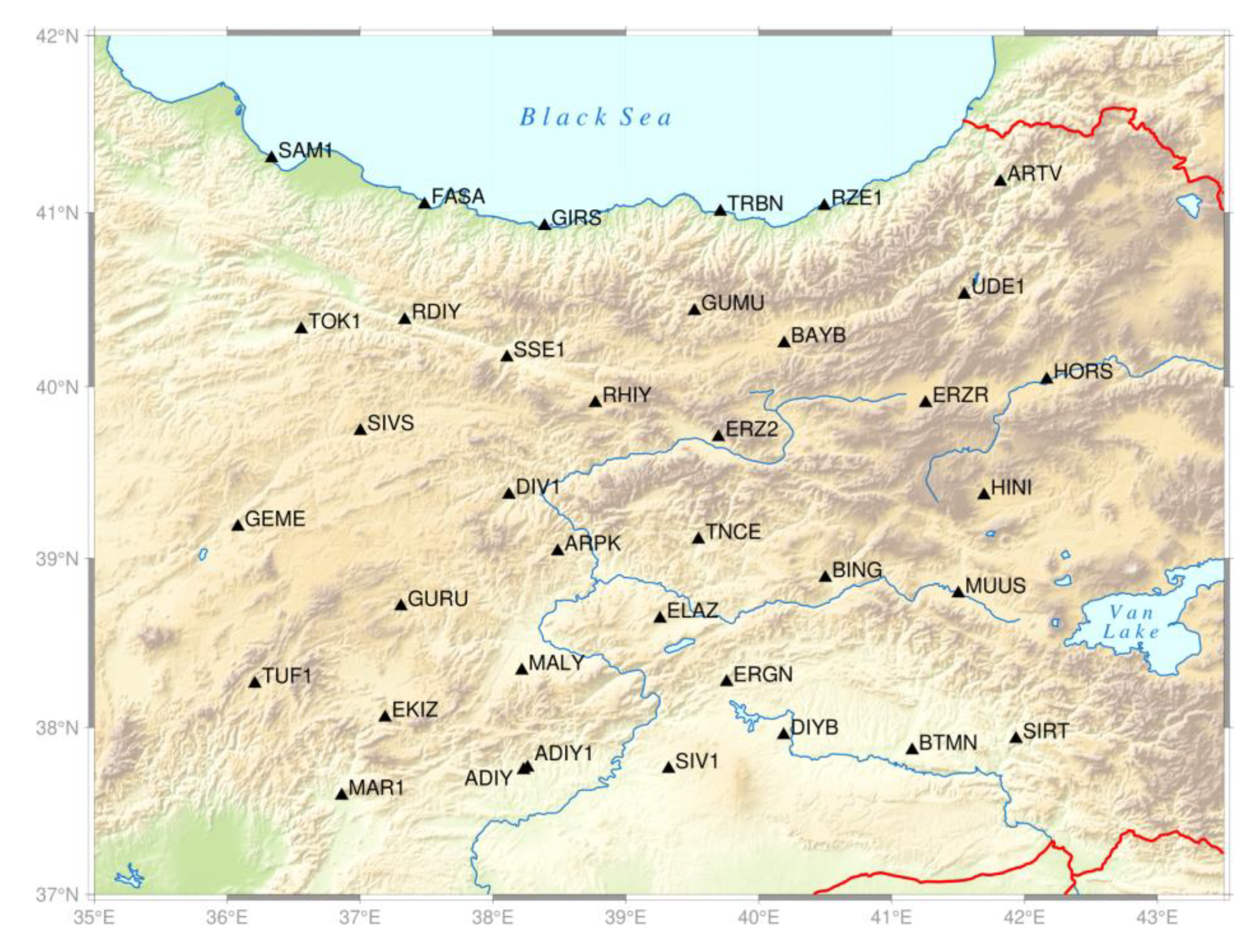
Figure 3.
Power frequency variation for GNSS stations with different ellipsoidal heights.
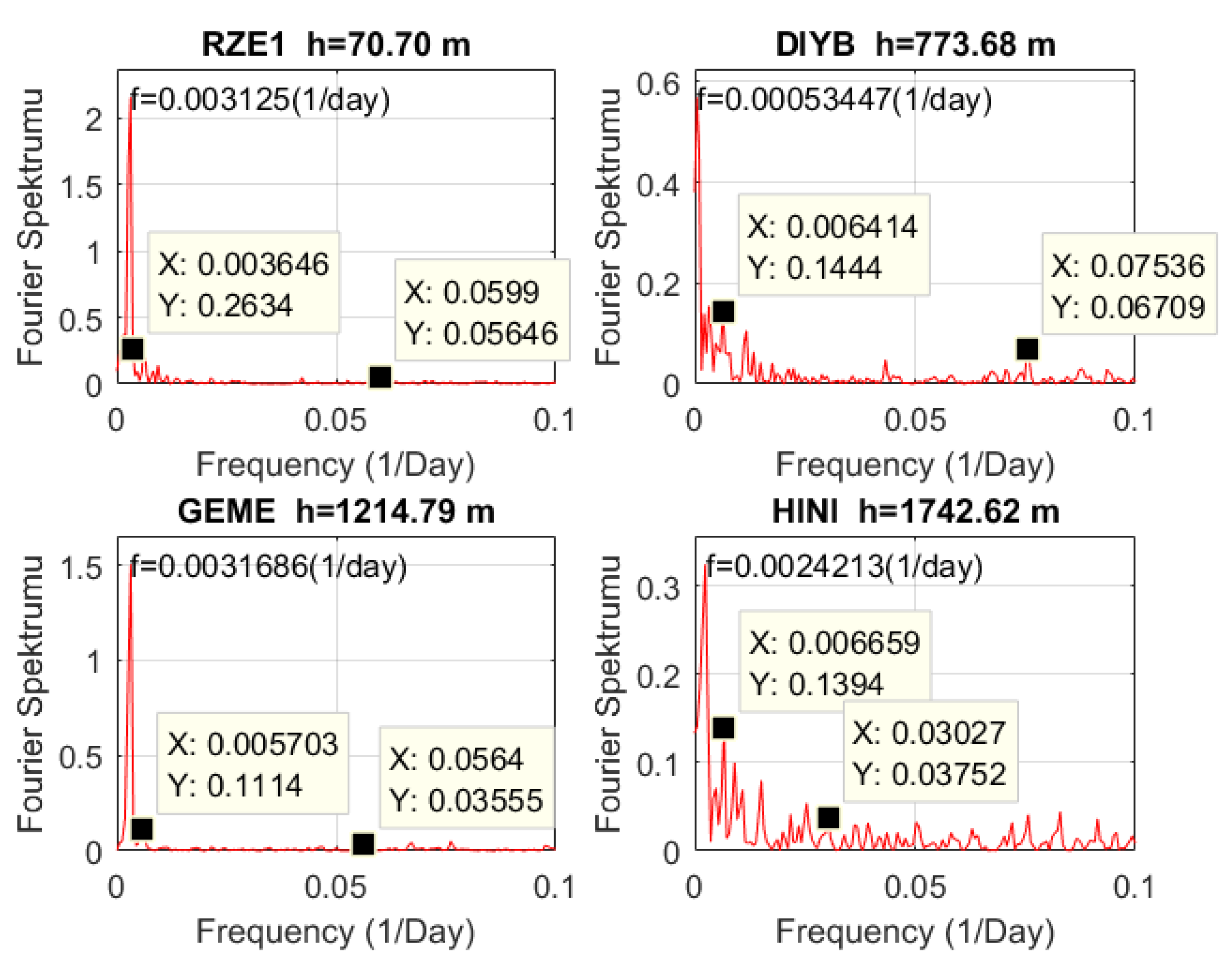
Figure 4.
ARMA model results for RZE1, DIYB, GEME, and HINI stations, respectively.
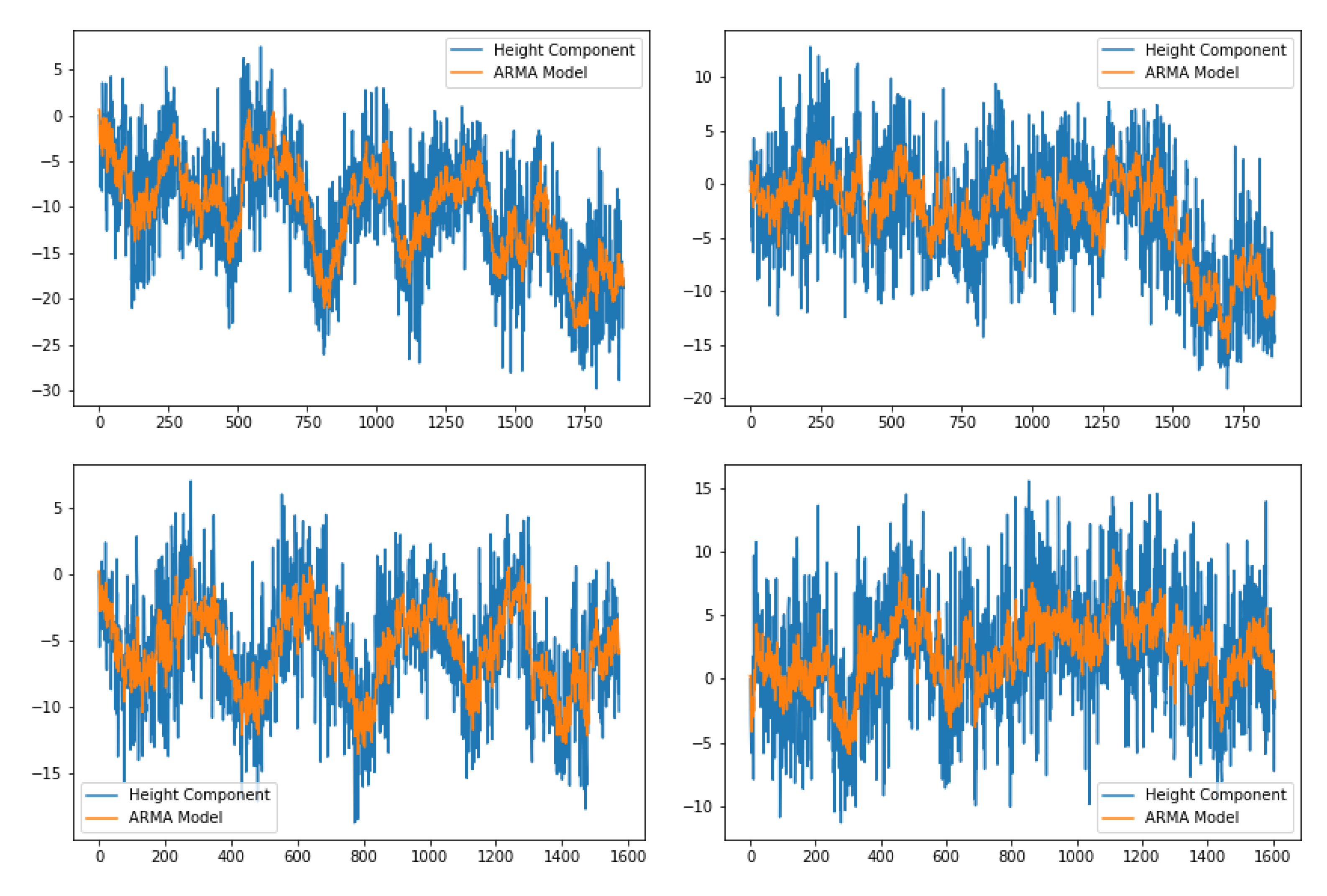
Figure 5.
The histograms of ARMA model residuals for RZE1, DIYB, GEME, and HINI stations, respectively.
Figure 5.
The histograms of ARMA model residuals for RZE1, DIYB, GEME, and HINI stations, respectively.

Figure 8.
The velocity and standard deviation depend on the observation time.
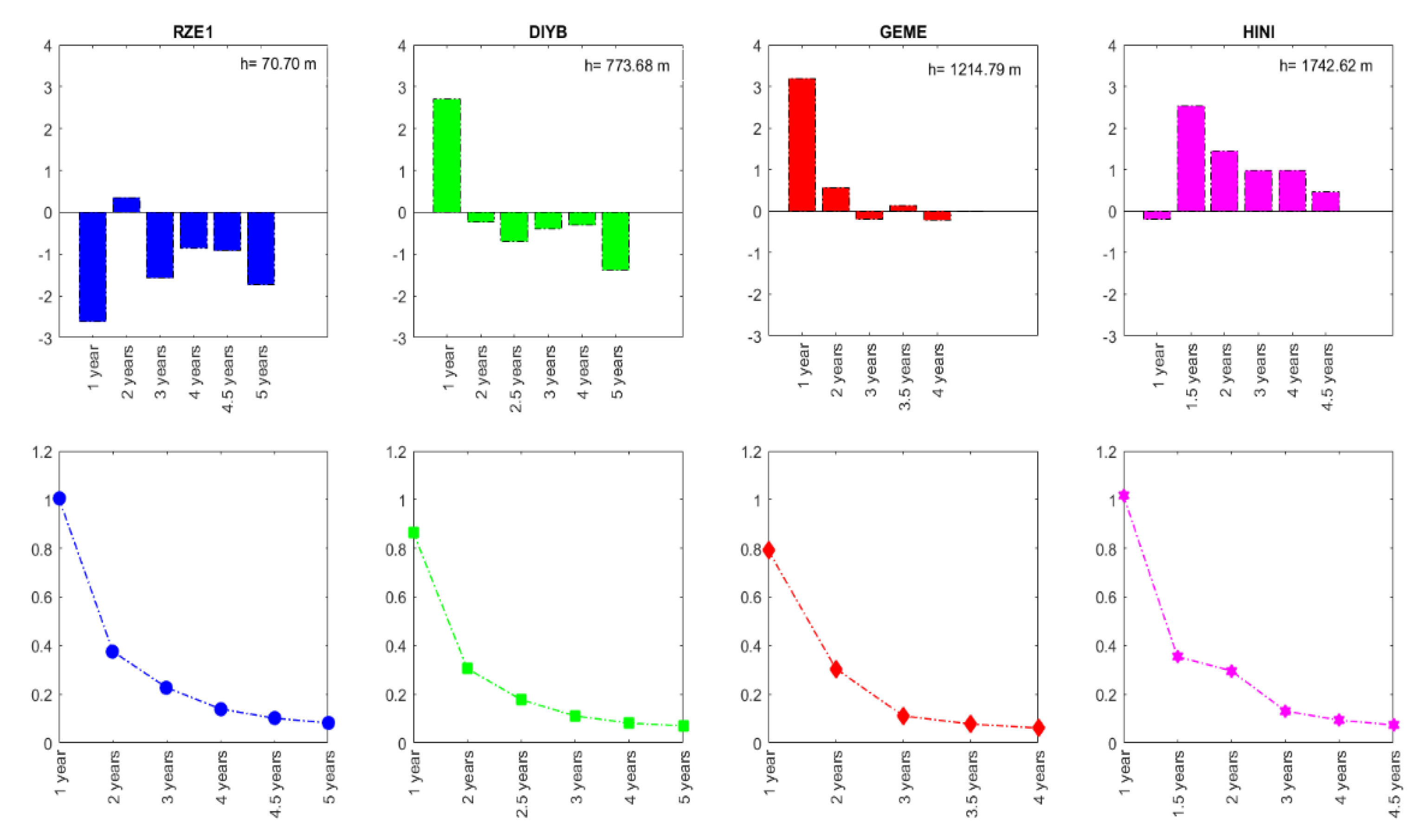
Figure 9.
Noise amplitudes for the height component of GNSS stations (mm).
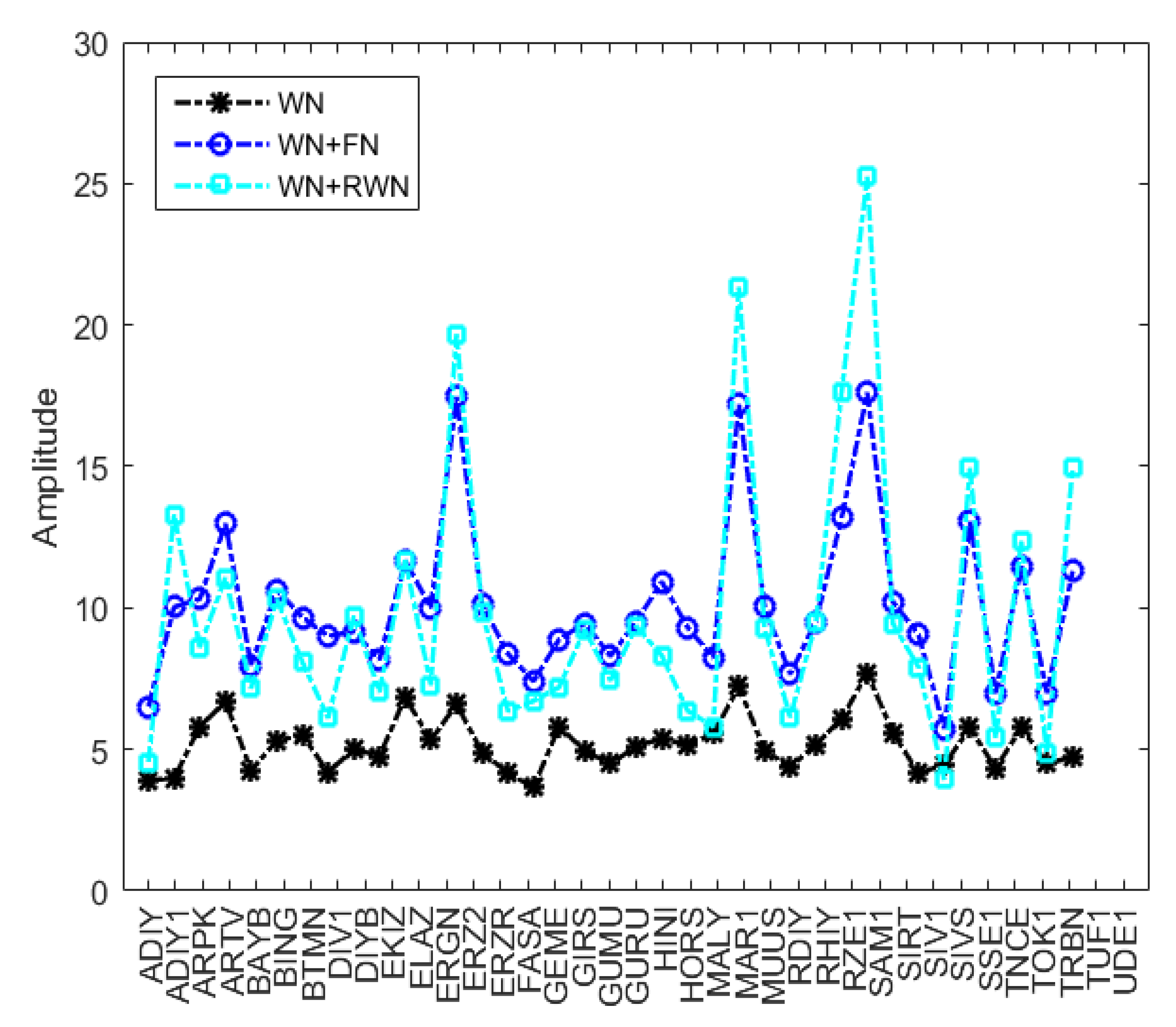
Figure 10.
Vertical velocities of GNSS stations (with standard deviation).
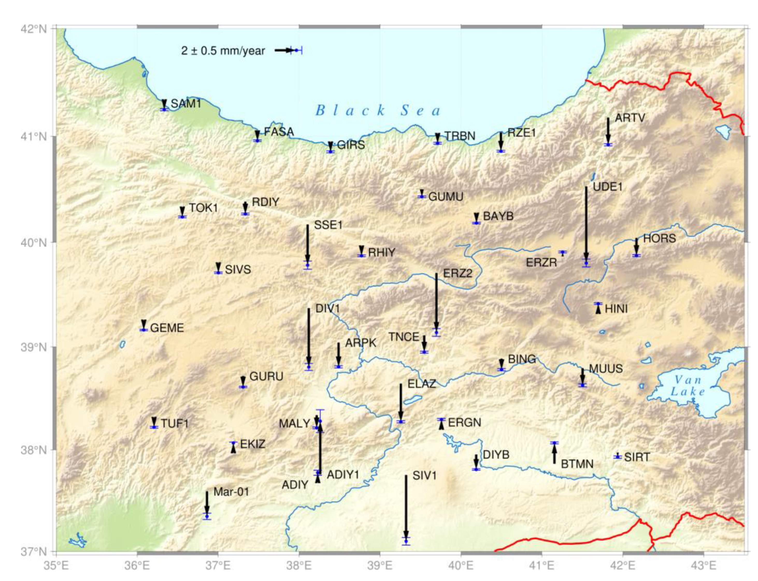
Table 1.
ARMA model results of all GNSS stations (mm).
| Station | RMSE | Station | RMSE | Station | RMSE |
|---|---|---|---|---|---|
| ARPK | 4.3 | FASA | 3.7 | RHIY | 4.0 |
| ARTV | 6.0 | GEME | 3.6 | RZE1 | 4.6 |
| BAYB | 3.8 | GIRS | 5.6 | SAM1 | 5.0 |
| BING | 4.5 | GUMU | 4.5 | SIRT1 | 5.8 |
| BTMN | 4.6 | GURU | 4.0 | SIV1 | 4.6 |
| DIYB | 4.6 | HINI | 4.7 | SIVS | 3.6 |
| EKIZ | 4.3 | HORS | 4.7 | SSE1 | 4.5 |
| ELAZ | 4.1 | MALY | 4.6 | TNCE | 4.4 |
| ERGN | 4.3 | MAR1 | 5.0 | TOK1 | 4.1 |
| ERZ2 | 5.9 | MUUS | 5.8 | TRBN | 5.2 |
| ERZR | 4.3 | RDIY | 4.3 | TUF1 | 4.3 |
Table 3.
MLE values for the height component of GNSS stations.
| Station Name | WN | WN+FN | WN+RWN |
|---|---|---|---|
| ADIY | -2055.88 | -2021.53 | -2030.47 |
| ADIY1 | -893.33 | -870.36 | -875.66 |
| ARPK | -6117.94 | -5522.66 | -5535.37 |
| ARTV | -6228.81 | -6058.52 | -6083.00 |
| BAYB | -5480.71 | -5263.38 | -5285.34 |
| BING | -5966.24 | -5649.25 | -5674.37 |
| BTMN | -5346.34 | -5025.07 | -5030.89 |
| DIV1 | -1862.70 | -1837.18 | -1849.91 |
| DIYB | -5674.47 | -5330.02 | -5348.08 |
| EKIZ | -5608.21 | -5380.61 | -5400.12 |
| ELAZ | -6552.98 | -5582.48 | -5595.51 |
| ERGN | -5862.46 | -5438.95 | -5460.24 |
| ERZ2 | -3044.00 | -2957.26 | -2982.03 |
| ERZR | -4878.81 | -4669.01 | -4693.86 |
| FASA | -4466.79 | -4367.48 | -4395.73 |
| GEME | -4286.05 | -4208.82 | -4238.10 |
| GIRS | -5560.61 | -5493.86 | -5511.82 |
| GUMU | -5710.76 | -5505.63 | -5529.03 |
| GURU | -5582.92 | -5346.43 | -5367.65 |
| HINI | -5039.06 | -4906.68 | -4923.73 |
| HORS | -4864.26 | -4651.58 | -4676.16 |
| MALY | -4938.48 | -4751.52 | -4767.68 |
| MAR1 | -2810.56 | -2715.46 | -2716.60 |
| MUUS | -5508.72 | -5128.36 | -5144.83 |
| RDIY | -5586.74 | -5326.16 | -5351.67 |
| RHIY | -5505.22 | -5290.85 | -5310.65 |
| RZE1 | -5883.08 | -5651.90 | -5666.65 |
| SAM1 | -6262.62 | -5906.24 | -5934.94 |
| SIRT | -6470.70 | -5907.66 | -5934.17 |
| SIV1 | -2292.51 | -2143.37 | -2144.46 |
| SIVS | -5274.21 | -5002.70 | -5037.81 |
| SSE1 | -1881.27 | -1871.78 | -1876.02 |
| TNCE | -6089.55 | -5600.75 | -5634.75 |
| TOK1 | -5262.40 | -5136.50 | -5154.79 |
| TRBN | -6005.57 | -5824.70 | -5849.34 |
| TUF1 | -5358.58 | -5248.94 | -5263.92 |
| UDE1 | -1754.19 | -1703.14 | -1715.38 |
Disclaimer/Publisher’s Note: The statements, opinions and data contained in all publications are solely those of the individual author(s) and contributor(s) and not of MDPI and/or the editor(s). MDPI and/or the editor(s) disclaim responsibility for any injury to people or property resulting from any ideas, methods, instructions or products referred to in the content. |
© 2023 by the authors. Licensee MDPI, Basel, Switzerland. This article is an open access article distributed under the terms and conditions of the Creative Commons Attribution (CC BY) license (http://creativecommons.org/licenses/by/4.0/).
Copyright: This open access article is published under a Creative Commons CC BY 4.0 license, which permit the free download, distribution, and reuse, provided that the author and preprint are cited in any reuse.


