
Submitted:
29 May 2023
Posted:
31 May 2023
You are already at the latest version
Abstract
In principle, modular or integral character of manufacturing lines depends on topological designs of products and determined operation tasks. On the other hand, in specific situations there is an articulated need for modular design in smart manufacturing systems, since modular layouts are a crucial step towards agile production via smart manufacturing. The aim of this paper is to explore how the modular layout relates to manufacturing lead time (MLT) and to operational complexity of smart manufacturing systems. For this purpose, topologically different models of alternative process layouts were simulated and tested, while MLT values were obtained using Tecnomatix Plant Simulation. Obtained positive findings of this research could be useful not only in selection of the most suitable process design from the alternative ones, but especially in deepening knowledge and better understanding of the concept of optimal network modularity.
Keywords:
process design
; modularity
; complexity
; manufacturing lead time
; simulation
1. Introduction
The idea of modularity is widely discussed and analyzed in diverse fields, e.g., in computer science, in neurophysiology, in evolutionary biology, in smart manufacturing systems, etc. It is due to the fact that modularity creates system information on different levels to support Industry 4.0 or smart manufacturing in a sustainable way [1]. In relation to manufacturing systems, modularity is considered as an effective approach, e.g., to minimize production costs [2], to increase flexibility of smart manufacturing systems [3], and to improve readiness for mass customization [4]. Therefore, modularity is seen as a tool that improves the productivity and efficiency of manufacturing processes. Especially in recent years, with the increasing importance of mass customization, modularity has become a popular topic in product and process development, since implementation of its principles [5] helps companies in organizing complex products and processes. In addition, process modularity allows to shorten cycle times, e.g., by organizing production as a modular consortium, the concept that was established in automotive industry since 1996 [6 - 8]. In this context, this study aims to explore the relation between process modularity and manufacturing lead time; and between process modularity and process complexity. The main goal of this research is focused on the following two research questions (RQs):
RQ 1: To what extent more modular process affects manufacturing lead time?
RQ 2: How more modular process affects the process complexity?
This article is organized in the following manner. Firstly, the related works are briefly described in the second section. Thereafter, the methodological framework describes the steps of the proposed approach. Subsequently, the selection of relevant indicators is provided together with demonstration of their application on a simple process example. Then, theoretical representative process models and realistic case study are introduced and used to explore the relationship between optimal modularity (OM) and MLT; and between OM and operational complexity of manufacturing processes. Finally, obtained results are summarized, and answers to the above mentioned research questions are provided.
2. Related Works
Modular approaches are increasingly being used as an integral part of design methods, as many systems, including products and processes, evolve toward increasing modularity [9]. Hölttä-Otto and Salonen [10] classify modular design methods into Design Structure Matrix (DSM), Modular Function Deployment (MFD), and Function Structure Heuristics (FSH). DSM methods aims to structurally describe system elements to cluster them into modules [11]. MFD approach consists of five stages that are aptly characterized, e.g., in work of Brunoe et al. [12]. FSH techniques developed by Stone et al. [13] include three strategies aimed for identifying modules for product architectures at the functional level.
Modularity a system property can be studied from many diverse perspectives. In contrast to specific views on modularity, generic insights attract more attention. One of them is that tweaking this system property can be seen as possible way in the course of system evolution as it slows its atrophy [14], but this effort shouldn't be endless and ineffectual. The effectiveness of such an effort also depends on the appropriateness of the modularity metrics used. There are several possible approaches how to evaluate product and process modularity as a relative measure of the degree of granularity, i.e. the level of detailization of the system element before or after its decomposition [15]. In other words, relative modularity can be defined as 'a measure quantifying the tendency of the network to be organized in network modules [16]. Such metrics (see, e.g., [17 - 20]) are used to compare this property among multiple designs. Several independent authors pointed out in their works [21 - 25] that over-modularization is as undesirable as un-der-modularization. They came to this conclusion by assessing advantages and disadvantages of these two contradictory solutions. Vanderfeesten et al. [26] stated that low system modularity in general can cause higher number of unwanted effects than the same system of high modularity. Moreover, in case of under-modularization, there are difficulties to maintain the large system elements or modules. On the other hand, disadvantage of over-modularization is a large number of linkages that need to be manage. A possible solution to overcome this issue is to identify accurate level of system granularity by an exact formula for quantifying this measure. According to Efatmaneshnik and Ryan [27], OM can be achieved 'through balanced modularization as structural symmetry in the distribution of the sizes of modules'. Kashkoush and ElMaraghy [28] proposed the optimal product modularity measure to obtain a product structure tree which ensures OM at all hierarchical levels. Talking about optimal modularity, it is important to mention well-known optimal network modularity indicator developed by Newman and Girvan [29], whose formula is described in section 4 of this paper.
The process modularity issues are often investigated in the context of process complexity (see, e.g., works of [30 –32]). Process modularity is considered as the degree to which a system is composed of relatively independent interacting elements encapsulated into modules that can be combined in variations to provide different functions [33]. Process complexity can be defined as the degree to which a process is complicated to analyze, study or understand [34]. It's apparent that both, process modularity and process complexity are important inherent system properties. It is also known that process modularity is primarily used to reduce its complexity by decomposing process into modules, as they are easier to manage as a whole [35]. The related problems were explored, e.g., in work [36], where authors identified a strong negative correlation between complexity and system modularity, and it confirms that lower complexity implies higher modularity. Although literature offers many complexity measures/indicators focused on product and process complexity (see, e.g., works of [37 - 41]), they are mostly usable for specific tasks. Bonchev and Buck [42] proposed several effective complexity measures which combines the adjacency and distance matrix of the network. Their methods are devoted to measure topological complexity and are easily applicable also in manufacturing process domain. Authors of the work [43] developed two practically oriented complexity indicators to assess assembly supply chain networks. It is also worth to mention a generic static complexity measure that is easily employed in manufacturing systems environment [44]. Input variables for this complexity measure need to be extracted from production orders and scheduling tasks. Moreover, there are several works which are focused on exploration of positive modularity impact on manufacturing lead time, e.g., [45 - 49].
3. Methodological Framework
In order to verify the working assumption that process modularity could positively impact on MLT and complexity of assembly process structures, the following methodical phases shown in Figure 1 will be applied.
4. Potential Indicators to Measure Process Modularity and Process Complexity
In this section, several indicators to measure process modularity and process complexity are described. Subsequently, the most suitable indicators for the mentioned the two system properties will be chosen.
4.1. Description of the Indicators to Measure Process Modularity
The four process modularity indices were considered for the given purposes. The first of them is called Singular Value Modularity Index (SMI). Although this measure was originally intended to enumerate the degree of product modularity, it is also applicable to measure process modularity. This index enumerates the degree of system modularity by employing singular value decomposition on the design structure matrix. For the given purpose the following equation was proposed [50]:
where N represents the number of system components; σi means singular value, where i = 1, 2, …, N-1.
The SMI measure can reach values between zero to one, while values closer to zero means a minimum degree of modularity, and vice versa.
The second indicator, the cross-module independence (CMI), calculates the ratio of the sum of relations inside all modules to the sum of all relations, and is expressed by the following equation [51]:
where n stands for the number of modules, while int = 1, 2, … , n; R represents the number of inside connections; and T is the number of all linkages in a network.
Third one – optimal modularity indicator Qd, proposed by Newman and Girvan [29] can be also used to identify optimal process structure from a set of alternative ones. This index is quantified by using equation:
where n indicates the number of modules, L represents the sum of all edges in a network, ls is the sum of internal edges in module s, wsout is the number of output edges in module s, and wsin stands for the number of input edges in module s.
The last considered indicator named as the optimal modularity indicator M(G) is aimed to measure the OM of process structures. This indicator is expressed as follows [52]:
where n is the number of modules in a network, Nj is the number of couplings extracted from columns of related visibility matrix, j = 1,…, K, while K is the number of columns in a related design matrix (see an example in Figure 3).
Principally, all the mention modularity indicators are more or less suitable for exploration of the relationships. However, it is possible to identify relevant differences in their sensitivity to recognize slight topological nuances when comparing similar process structures. These differences were already studied in our previous work [52], where the indicator M(G) was prioritized against the concurrent ones. Therefor it will be used for intended purpose in this study.
4.2. Description of the Indicators to Measure Process Complexity
The four complexity indicators are assumed below for the purpose to select the most suitable one from them.
Deshmukh et al. [44] developed a formula to measure the complexity of manufacturing systems that is expressed as follows:
where n is the number of parts, m is the number of operations, while r is the number of machines.
The second indicator is based on the concept of Shannon’s information entropy and it is formulated through the following equation [53]:
where M is the number of machines, S stands for the number of possible planned states of the machine j can be in, pij is probability that the machine j is in state i.
The third one, so-called modified flow complexity (MFC) indicator enumerates all tiers, nodes, and links weighted with determined α, β, and γ coefficients. This indicator is enumerated using formula [54]:
where α is multi-tier coefficient (α ≥ 0), β reflects network nodes (β ≥ 0), γ is manufacturing network links coefficient (γ ≥ 0); N is the number of nodes; L is number of links; and T is the number of tiers.
The forth indicator is devoted to measure operational complexity of manufacturing systems. This indicator is calculated using the following equation [55]:
where pijk is probability that part j is being proceeded due to operation k by individual machine i according to scheduling order, O is the number of operations, P means the number of parts produced in manufacturing process, M is the number of all machines in manufacturing process.
Based on the recent comparisons of the alternative complexity measures [54], indicator PCI was selected for measuring the operational process complexity.
5. Procedures to Calculate Modularity, Complexity and MLT
To show application procedures for using the selected indicators (M(G), PCI), and MLT, the following two sub-sections provide simple demonstrations, how it works.
5.1. Procedures for M(G) and PCI
Firstly, let us have a model of manufacturing process, in which parts P1, P2 and P3 are processed by machines M1, M2, M3, M4, M5, M6 and M7, and scheduled as it is depicted in Figure 2.
When applying M(G) indicator, at first, it is needed to create visibility matrix of the given process model (see in Figure 3) to obtain Nj values.
Figure 3.
Visibility matrix of the manufacturing process.
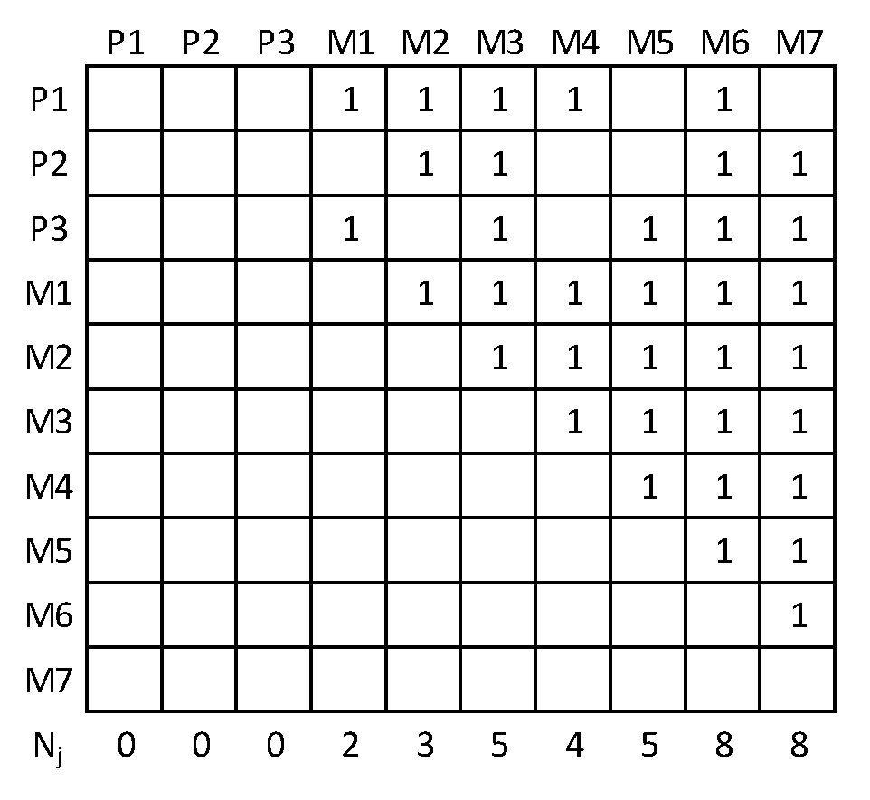
Then, process modularity is quantified using equation (4) as follows:
The procedure is repeated for all alternative structure models. Then, the model with the highest M(G) value represents the optimal manufacturing process structure among concurrent ones from the modularity point of view.
In order to apply of PCI indicator, at first, it is necessary to enumerate partial complexities of the machines. Then, their sum represents the overall complexity of the process. Let us demonstrate enumeration of partial complexity for machine M1 by applying formula (8). This machine is processing two parts (P1 and P3), and therefore the partial complexity of M1 has to be enumerate in this way:
where, e.g., p11 is probability that part P1 is just being proceeded by machine M1. It needs to be noticed that when this part is processed on machines in serial manner, then p11 equals 1/5, because number of machines in serial connection equals five.
The partial complexities can be enumerated in the two ways as shown in Figure 4. Due to this fact, it is possible to create graph of complexity distributions, where the resulting cumulated complexities are the same for both the views. It can be easily proved that PCI value for the given process model is 7,04 bits.
5.2. Procedure to Enumerate MLT
In order to generate MLT values, simulation software was employed. Manufacturing lead time is defined as the total time required to process a product through the plant, and its formal definition was given by Groover [56]:
where j stands for part number or product number; Tsuij is setup time for operation i on part or product j; Qj is quantity of part or product j in the batch being processed; Tcij is cycle time for operation i on part or product j; Ttij is transport time associated with operation i, where i indicates the operation sequence in the processing, i = 1, 2, …, noj.
Moreover, it is needed to know set-up times, processing cycle times and transport times. The allocated setup time is three seconds, and processing cycle time equals one minute for all seven machines. Transport times are assigned based on the distance between the machines. Specifically, five seconds are assigned between two machines located next to each other (e.g. M1 to M2); and ten seconds are set up between machines located not close to each other (e.g. M1 and M3). Obtained total MLT for all the parts using simulation software is 6 minutes and 53 seconds (see Figure 5).
6. Testing and Analysis of the Indicators through Theoretical Process Models
For this purpose, process models from work by Latva-Koivisto [57] who explored complexity of six Kaimann's process graphs [58] were used for the theoretical experiment. It is assumed that 100 parts are produced on 22 machines (see Figure 6). In addition, set-up times, processing cycle times and transport times were assigned. The allocated set-up time was two seconds, and processing cycle time was one minute for all the 22 machines. Transport times were assigned based on the distance between the machines. Five seconds between two machines located next to each other (e.g. M2 to M3); ten seconds between machines, e.g., M2 and M9; and 15 second between machines that are located further away from each other (e.g. M2 and M15).
Process modularity and complexity values were enumerated using equations (4) and (8), while MLT values were obtained using the simulation tool. The obtained values are summarized in Table 1.
Following the obtained results, one can see when comparing process modularity and MLT, that process modularity of Graph 1 is the highest while its MLT is the shortest. Process modularity of the remaining graphs has the same tendency in relation to MLT values. Then, it is possible to state from these summarized results, that modularity values are in relation with MLT values - as the modularity increases, MLT decreases, and vice versa. When comparing process modularity in relation to operational complexity, it can be seen that Graph 1 has the lowest complexity, while its process modularity is the highest. The rest of graphs report the same tendency, and it can be said that OM positively impacts on operational complexity of manufacturing systems.
To answer research questions mentioned in the introduction section and to confirm the positive impact of process modularity on MLT and process complexity, the two methods are further employed to find to what extent the OM effects on MLT, and how modularity influences the process complexity of manufacturing systems.
As first, the Spearman correlation analysis was used to test these relationships. Spearman correlation coefficient rated using known scale [59] between OM and manufacturing lead time; and between OM and process complexity equals - 0,91 and – 0,98, respectively. Based on these results, it means that there are very strong relationships.
Then, the sensitivity index ”I” is used to assess sensitivity between the M(G) and MLT values, as well as between M(G) and PCI values. For this purpose, the following formula will be applied [60].
where y0 is the model output calculated with an initial value x0 of the parameter x; x1 = x0 - ∆x and x2 = x0 + ∆x with corresponding values y1 and y2.
Sensitivity values are ranked into four classes, small to negligible sensitivity (0 ≤ |I | ˂ 0,05); medium sensitivity (0,05 ≤ |I | ˂ 0,20); high sensitivity (0,20 ≤ |I | ˂ 1); very high sensitivity (|I | ≥ 1).
By applying formula (10) for all the six process structures, the following values are obtained: I = - 7,37 between M(G) and MLT, and I = - 1,55 between M(G) and PCI. Based on the obtained results, it can be said that in the both relationships there are very high sensitivities.
These two relationships will be also tested on the realistic case study in the next section.
7. Case Study
The case study is focused on production of the bicycle frames consisting of 11 parts (P) machined on the 37 machines (M). Five manufacturing process alternatives are compared, where one of them consists of two production lines (PLs), the two of them are created from three production lines, one alternative consists of four PLs, and the last one produces the products through six production lines. First-in-first-out scheduling algorithm is used for this purpose.
Sequence of machines and their operational times are shown in the following Table 2.
To identify MLT values by simulation tool, set-up times and transport times will be also assumed. Set-up time equals 10 seconds for all the machines. Transport times between all the machines located next to each other will be the same (5 seconds). The rest of transport times are assigned by simulation tool based on the distance between machines (see Table 3).
7.1. Description of Process Structures
Process design alternative ”A” (see Figure 7a) consist of 37 machines divided into two PLs. Parts P3 – P11 pass through the first production line, while parts P4, P8, P10 and P11 are finalized in the second one. Parts P1 and P2 are produced only in the second line.
Process design alternative ”B” (see Figure 7b) contains three PLs. Parts P4, P8, P9, P10 and P11 pass through the first PL, while parts P4, P8, P10 and P11 are finalized in the second PL. Parts P1 and P2 are produced in the second PL and remaining parts are processed in PL #3.
Process design alternative ”C” (see Figure 8a) is divided also into three PLs. The first production line processes parts P8, P9, P10 and P11, but parts P8, P10 and P11 are finalized in the second PL together with parts P1 and P2. Parts P3-P7 pass through the last production line #3.
Process design alternative ”D” (see Figure 8b) consists of four production lines. Parts P4, P9 and P11 are processed in the first one PL, while parts P4 and P11 are finally processed in the second PL together with parts P8 and P10, which are finalized in the next line together with P1 and P2. Parts P3, P5, P6 and P7 pass through the fourth production line.
Process design alternative ”E” (see Figure 8c) contains six production lines. Part P4 passes firstly through the first line and then, it is finalized in the fifth PL. Parts P9 and P11 are processed in the second PL, but P11 is finalized in the fifth PL. Parts 8 and P10 are firstly produced in the third PL, but they are finalized also in the fifth PL. Parts P1 and P2 pass firstly through the fourth PL and they are finalized in the last PL. Parts P3, P5, P6 and P7 are processed only in the last production line.
7.2. Analysis of Results
All the five process structures were assessed using above introduced optimal modularity indicator M(G) and operational complexity indicator PCI and also tested through simulation software to obtain MLT values. Obtained results for all the alternatives are depicted in Table 4.
When comparing process modularity values and MLT values, it is possible to state that there is the following relationship. If the modularity increases, then MLT decreases, and vice versa. When comparing process modularity in relation to operational complexity, it can be seen that Alt. ”E” has the lowest complexity, while its process modularity is the highest. The rest of process models are subject to the same tendency and it can be said that OM positively impacts on operational complexity of manufacturing systems.
To confirm or deny the previous statements (from Section 6) to the RQs, the Spearman correlation analysis and the sensitivity analysis were applied.
The Spearman correlation analysis confirmed very strong negative relationships (ρ = - 0,82) between M(G) and MLT values, and between M(G) and PCI values as ρ = - 0,87.
Sensitivity index between M(G) and MLT enumerated using equation (10) equals – 47,17; and between M(G) and PCI values is - 6,13. Based on the obtained results, it can be said that there is very high sensitivity between these two relationships.
8. Conclusion
When exploring specific practical modularity problems, it seems to be useful to stress that the first important task is to select appropriate method(s) to assess this system attribute. For the purpose of this study, the optimal modularity indicator M(G) has been applied along with the operational complexity indicator (PCI) and MLT indicator. The second precondition to deal with this issue is to take adequate process models to carry out experiments. We tried to fulfill these two conditions consistently.
As the purpose of this study is linked to the research questions presented in the introduction section, we provide the following summarized answers to them, although partially it was done in sections 6 and 7:
- Answer to RQ 1: Considering the achieved results presented in sections six and seven, one can state that process structure modularity positively affects the manufacturing lead time in this sense that if manufacturing process modularity increases, then MLT decreases, what was proved in both the testing cases.
The answer to the question regarding to what extent modularity can impact MLT, it is purposeful to quantify percentage change of MLT caused due to modularity using the both simulation experiments. Then, one can easily find that difference of MLT between less and more modular manufacturing process is: 4,8 % in case of theoretical process models, 2% in case of real process models.
- Answer to RQ 2: Taking into account the obtained results from the experiments, it can be stated that process structure modularity positively affects the complexity of manufacturing processes, so that if manufacturing process modularity in-creases, then process complexity decreases. These rigorously obtained results prove the statement that the concept of modularity is purpose-built to reduce complexity by breaking a system into varying degrees of interdependence [61].
Finally, potential future research directions could be directed to explore the influence of process modularity on smart mass customization assembly systems with the aim to validate presented findings with a higher degree of generality.
Author Contributions
Conceptualization, V.M.; methodology, V.M. and Z.S.; software, Z.S.; validation, Z.S., formal analysis, Z.S.; writing—original draft preparation, Z.S.; writing—review and editing, V.M.; visualization, Z.S.; supervision, V.M.
Funding
This research has been funded by the project SME 5.0 with funding received from the European Union’s Horizon research and innovation program under the Marie Skłodowska-Curie Grant Agreement No. 101086487 and the KEGA project No. 044TUKE-4/2023 granted by the Ministry of Education of the Slovak Republic.
Institutional Review Board Statement
Not applicable.
Informed Consent Statement
Not applicable.
Conflicts of Interest
The authors declare no conflict of interest.
References
- Habib, T.; Omair, M.; Habib, M. S.; Zahir, M. Z.; Khattak, S. B.; Yook, S. J.; Akhtar, R. Modular Product Architecture for Sustainable Flexible Manufacturing in Industry 4.0: The Case of 3D Printer and Electric Toothbrush. Sustainability 2023, 15. [Google Scholar] [CrossRef]
- ElMaraghy, H.; Schuh, G.; ElMaraghy, W.; Piller, F.; Schönsleben, P.; Tseng, M.; Bernard, A. Product variety management. Cirp Annals 2013, 62, 629–652. [Google Scholar] [CrossRef]
- Massimi, E.; Khezri, A.; Benderbal, H. H.; Benyoucef, L. A heuristic-based non-linear mixed integer approach for optimizing modularity and integrability in a sustainable reconfigurable manufacturing environment. The International Journal of Advanced Manufacturing Technology 2020, 108, 1997–2020. [Google Scholar] [CrossRef]
- Pishdad, A.; Taghiyareh, F. Mass customization strategy development by FIRM. Journal of Database Marketing & Customer Strategy Management 2011, 18, 254–273. [Google Scholar]
- Anssen, F.; Grossman, P.; Westbroek, H. Facilitating decomposition and recomposition in practice-based teacher education: The power of modularity. Teaching and teacher education 2015, 51, 137–146. [Google Scholar] [CrossRef]
- Collins, R.; Bechler, K.; Pires, S. Outsourcing in the automotive industry: from JIT to modular consortia. European management journal 1997, 15, 498–508. [Google Scholar] [CrossRef]
- Pires, S. R. Managerial implications of the modular consortium model in a Brazilian automotive plant. International Journal of Operations & Production Management 1998, 18, 221–232. [Google Scholar]
- Miguel, P. A. C. Modularity in product development: a literature review towards a research agenda. Product: Management and Development 2005, 3, 165–174. [Google Scholar]
- Schilling, M. A. Toward a general modular systems theory and its application to interfirm product modularity. Academy of management review 2000, 25.2, 312–334. [Google Scholar] [CrossRef]
- Holtta, K. M.; Salonen, M. P. Comparing three different modularity methods. International Design Engineering Technical Conferences and Computers and Information in Engineering Conference 2003, 37017, 533–541. [Google Scholar]
- Eppinger, S. D.; Browning, T. R. Design structure matrix methods and applications; MIT press, 2012. [Google Scholar]
- Brunoe, T. D.; Soerensen, D. G.; Nielsen, K. Modular design method for reconfigurable manufacturing systems. Procedia CIRP 2021, 104, 1275–1279. [Google Scholar] [CrossRef]
- Stone, R. B.; Wood, K. L.; Crawford, R. H. A heuristic method for identifying modules for product architectures. Design studies 2000, 21, 5–31. [Google Scholar] [CrossRef]
- Tiwana, A.; Safadi, H. Atrophy in Aging Systems: Evidence, Dynamics, and Antidote. Information Systems Research 2023. [CrossRef]
- Yao, Y. A triarchic theory of granular computing. Granular Computing 2016, 1, 145–157. [Google Scholar] [CrossRef]
- Holme, P. Signatures of currency vertices. Journal of the Physical Society of Japan 2009, 78, 034801. [Google Scholar] [CrossRef]
- Blackenfelt, M. Managing complexity by product modularization. Doctoral dissertation, Royal Institute of Technology, Sweden, 2001. [Google Scholar]
- Modrak, V.; Soltysova, Z. Development of the Modularity Measure for Assembly Process Structures. Mathematical Problems in Engineering 2021. [Google Scholar] [CrossRef]
- Tran, T. D.; Kwon, Y. K. The relationship between modularity and robustness in signalling networks. Journal of The Royal Society Interface 2013, 10. [Google Scholar] [CrossRef]
- Larses, O.; Blackenfelt, M. Relational reasoning supported by quantitative methods for product modularization. DS 31: Proceedings of ICED 03, the 14th International Conference on Engineering Design Stockholm; 2003; pp. 347–348. [Google Scholar]
- Ethiraj, S. K.; Levinthal, D. A. Modularity and innovation in complex systems. Manage Sci 2004, 50, 159–173. [Google Scholar] [CrossRef]
- Geisendorf, S. Searching NK fitness landscapes: on the trade-off between speed and quality in complex problem solving. Comput Econ 2010, 35, 395–406. [Google Scholar] [CrossRef]
- Dosi, G.; Mareng, L. Division of labor, organizational coordination and market mechanisms in collective problem-solving. J Econ Behav Organ 2005, 58, 303–326. [Google Scholar]
- Brusoni, S.; Marengo, L.; Prencipe, A.; Valente, M. The value and costs of modularity: a problem-solving perspective. Eur Manage Rev 2007, 4, 121–132. [Google Scholar] [CrossRef]
- Conte, S. D.; Dunsmore, H. E.; Shen, V. Y. Software Engineering Metrics and Models. Benjamin-Cummings, Reading, Mass. 1986. [Google Scholar]
- Vanderfeesten, I.; Reijers, H.A.; Van der Aalst, W.M. Evaluating workflow process designs using cohesion and coupling metrics. BPM reports 2007, 0702, BPMcenter. [Google Scholar] [CrossRef]
- Efatmaneshnik, M.; Ryan, M. J. On optimal modularity for system construction. Complexity 2016, 21, 176–189. [Google Scholar] [CrossRef]
- Kashkoush, M.; ElMaraghy, H. Optimum overall product modularity. Procedia CIRP 2016, 44, 55–60. [Google Scholar] [CrossRef]
- Newman, M. E. J.; Girvan, M. Finding and evaluating community structure in networks. Physical Review E. 2004, 69, 1–16. [Google Scholar] [CrossRef] [PubMed]
- Vickery, S. K.; Koufteros, X.; Dröge, C.; Calantone, R. Product modularity, process modularity, and new product introduction performance: does complexity matter? Production and Operations management 2016, 25, 751–770. [Google Scholar] [CrossRef]
- Baldwin, C. Y.; Clark, K. B. Managing in an age of modularity. Managing in the modular age: Architectures, networks, and organizations 2003, 149, 84–93. [Google Scholar]
- Araujo, L.; Spring, M. Complex Performance, Process Modularity, and the Spatial Confi guration of Production. In Procuring Complex Performance; Routledge, 2010; pp. 94–112. [Google Scholar]
- Sinha, K.; Suh, E. S.; de Weck, O. Integrative complexity: an alternative measure for system modularity. Journal of Mechanical Design 2018, 140, 051101. [Google Scholar] [CrossRef]
- Cardoso, J. Evaluating the process control-flow complexity measure. IEEE International Conference on Web Services (ICWS'05). IEEE 2005.
- Yassine, A. A.; Naoum-Sawaya, J. Architecture, Performance, and Investment in Product Development Networks. ASME J. Mech. Des. 2016, 139, 011101. [Google Scholar] [CrossRef]
- Sinha, K.; Suh, E. S.; de Weck, O. Correlating integrative complexity with system modularity. In International design engineering technical conferences and computers and information in engineering conference 2017; American Society of Mechanical Engineers, 8127; Volume 58127, p. V02AT03A048. [Google Scholar]
- Zhang, Z.; Luo, Q. A grey measurement of product complexity. IEEE International Conference on Systems, Man and Cybernetics. IEEE 2007, 2176–2180. [Google Scholar]
- Zhang, X.; Thomson, V. A knowledge-based measure of product complexity. Computers & Industrial Engineering 2018, 115, 80–87. [Google Scholar]
- Frendall, L. D.; Gabriel, T. J. Manufacturing complexity: A quantitative measure. Proceedings of the POMS Conference 2003, Savannah, GA, USA, 4-7.
- Gabrie, I. H.; Shikdar, A. Design for manufacturing systems complexity: a perspective approach. Engineering Systems Design and Analysis 2010, 751–762. [Google Scholar]
- Phukan, A.; Kalava, M.; Prabhu, V. Complexity metrics for manufacturing control architectures based on software and information flow. Computers & Industrial Engineering 2005, 49, 1–20. [Google Scholar]
- Bonchev, D.; Buck, G. A. Quantitative measures of network complexity. In Complexity in Chemistry, Biology and Ecology; Bonchev, D., Rouvray, D.H., Eds.; Springer: New York, NY, USA, 2005; pp. 191–235. [Google Scholar]
- Modrak, V.; Marton, D.; Kulpa, W.; Hricova, R. Unraveling complexity in assembly supply chain networks. 4th IEEE International Symposium on Logistics and Industrial Informatics 2012, 151–156. [Google Scholar]
- Deshmukh, A. V.; Talavage, J. J.; Barash, M. M. Complexity in manufacturing systems, Part 1: Analysis of static complexity. IIE transactions 1998, 30, 645–655. [Google Scholar] [CrossRef]
- Watanabe, C.; Ane, B. K. Constructing a virtuous cycle of manufacturing agility: concurrent roles of modularity in improving agility and reducing lead time. Technovation 2004, 24, 573–583. [Google Scholar] [CrossRef]
- Zidi, S.; Hamani, N.; Kermad, L. Modularity metric in reconfigurable supply chain. Advances in Production Management Systems. Artificial Intelligence for Sustainable and Resilient Production Systems: IFIP WG 5.7 International Conference, APMS 2021, Nantes, France, September 5–9, 2021, Proceedings, Part V, Springer International Publishing, 455-464. 5 September.
- Chiu, M. C.; Okudan, G. L. E. An Investigation of Product Modularity and Supply Chain Performance at the Product Design Stage. International Design Engineering Technical Conferences and Computers and Information in Engineering Conference 2011, 54860, 681–689. [Google Scholar]
- Shamsuzzoha, A.; Piya, S.; Al-Kindi, M.; Al-Hinai, N. Metrics of product modularity: les-sons learned from case companies. Journal of Modelling in Management 2018, 13, 331–350. [Google Scholar] [CrossRef]
- Modrak, V.; Soltysova, Z. Batch size optimization of multi-stage flow lines in terms of mass customization. Int. J. Simul. Model 2020, 19, 219–230. [Google Scholar] [CrossRef]
- Holtta, K.; Suh, E. S.; de Weck, O. Tradeoff between modularity and performance for engineered systems and products. ICED 05: 15th International Conference on Engineering Design: Engineering. 2005; 449–450. [Google Scholar]
- Abdelkafy, N. Variety induced complexity in mass customization: Concepts and management 2008.
- Modrak, V.; Soltysova, Z. Exploration of the optimal modularity in assembly line design. Scientific Reports 2022, 12, 20414. [Google Scholar] [CrossRef] [PubMed]
- Frizelle, G.; Woodcock, E. Measuring complexity as an aid to developing operational strategy. International Journal of Operations and Production Management 1995, 15, 26–39. [Google Scholar] [CrossRef]
- Crippa, R.; Bertacci, N.; Larghi, L. Representing and measuring flow complexity in the extended enterprise: The D4G approach. In Proceedings of the RIRL 2006—Sixth International Congress of Logistics Research, Pontremoli, Italy, 3–6 September 2006. [Google Scholar]
- Modrak, V.; Soltysova, Z. Development of operational complexity measure for selection of optimal layout design alternative. International Journal of Production Research 2018, 56, 7280–7295. [Google Scholar] [CrossRef]
- Groover, M. P. Automation, Production Systems, and Computer-Integrated Manufacturing, 4th ed.; Pearson: London, 2016; pp. 1–816. [Google Scholar]
- Latva-Koivisto, A. M. Finding a complexity measure for business process models 2001.
- Kaimann, R. A. Coefficient of Network Complexity and Coefficient of Network Complexity: Erratum. Management Science 1974, 21, 172–177. [Google Scholar] [CrossRef]
- Dancey, C.; Reidy, J. Statistics without Maths for Psychology: using SPSS for Windows. PrenticeHall 2004, London. [Google Scholar]
- Lenhart, T.; Eckhardt, K.; Fohrer, N.; Frede, H. G. Comparison of two different approaches of sensitivity analysis. Physics and Chemistry of the Earth 2002, 27, 645–654. [Google Scholar] [CrossRef]
- Baldwin, C. Y.; Clark, K. B. Design rules, Volume 1: The power of modularity; MIT Press: Cambridge, Massachusetts, 2000. [Google Scholar]
Figure 1.
Applied methodological framework.
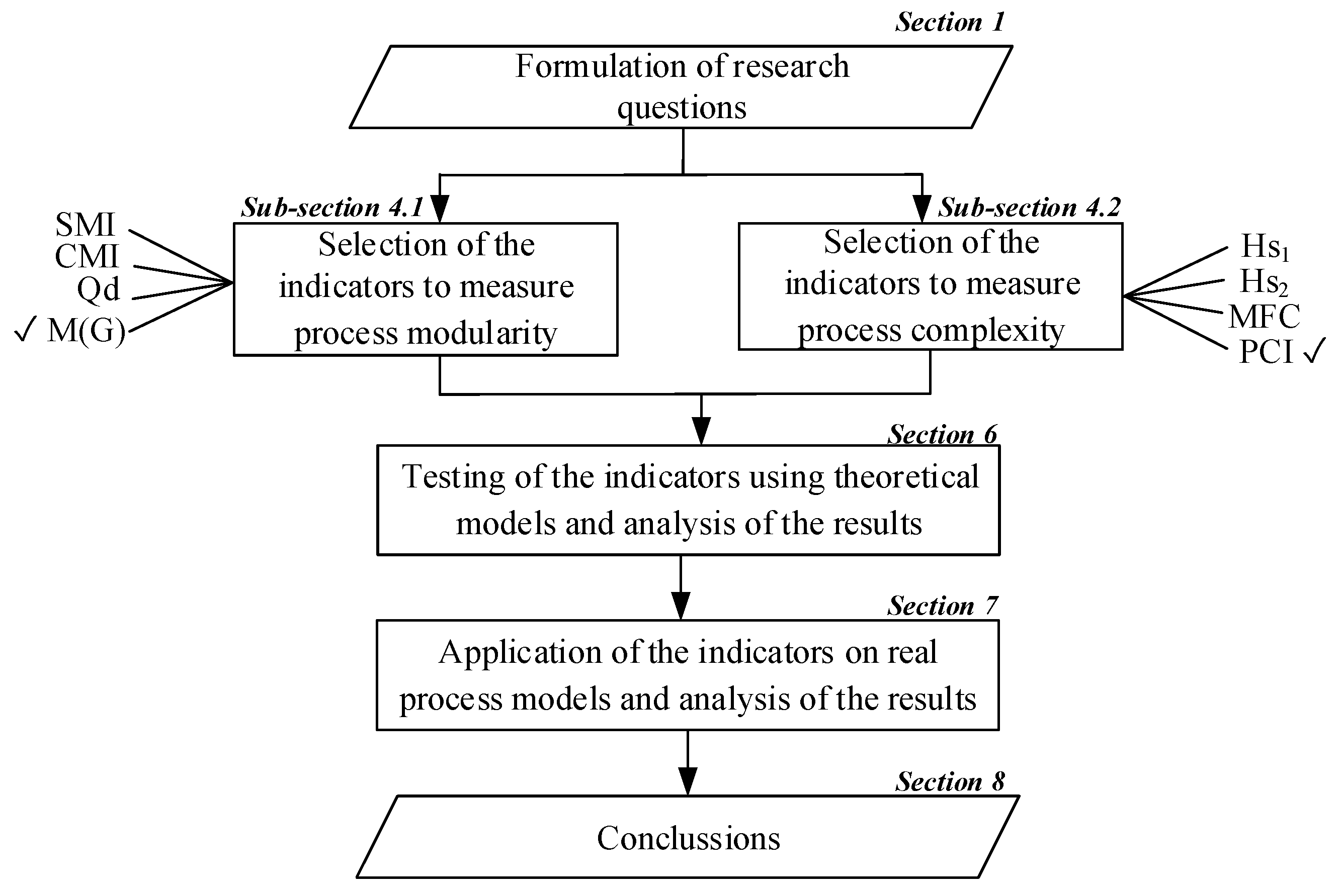
Figure 2.
A model of manufacturing process producing parts P1, P2 and P3.
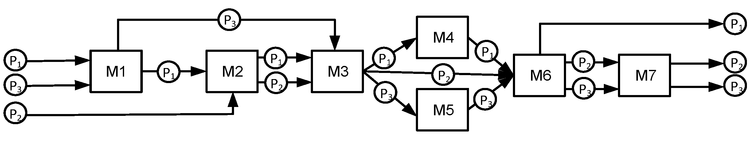
Figure 4.
a) Probabilities (pijk) and related complexity values; b) Partial complexities from the machine view and part view, and cumulated complexities of machines and parts production.
Figure 4.
a) Probabilities (pijk) and related complexity values; b) Partial complexities from the machine view and part view, and cumulated complexities of machines and parts production.
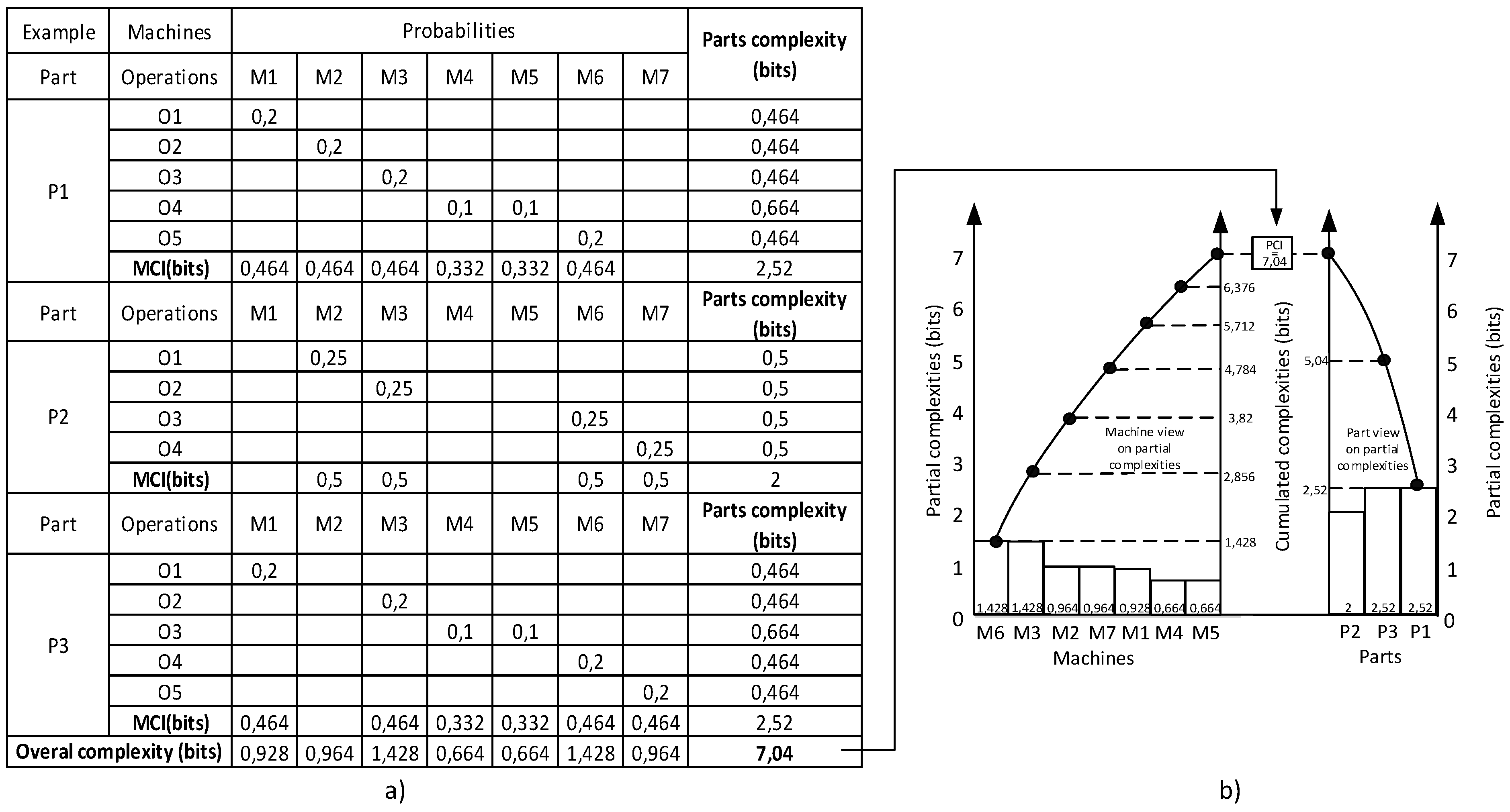
Figure 5.
Print screen of the selected process model from Tecnomatix Plant Simulation.
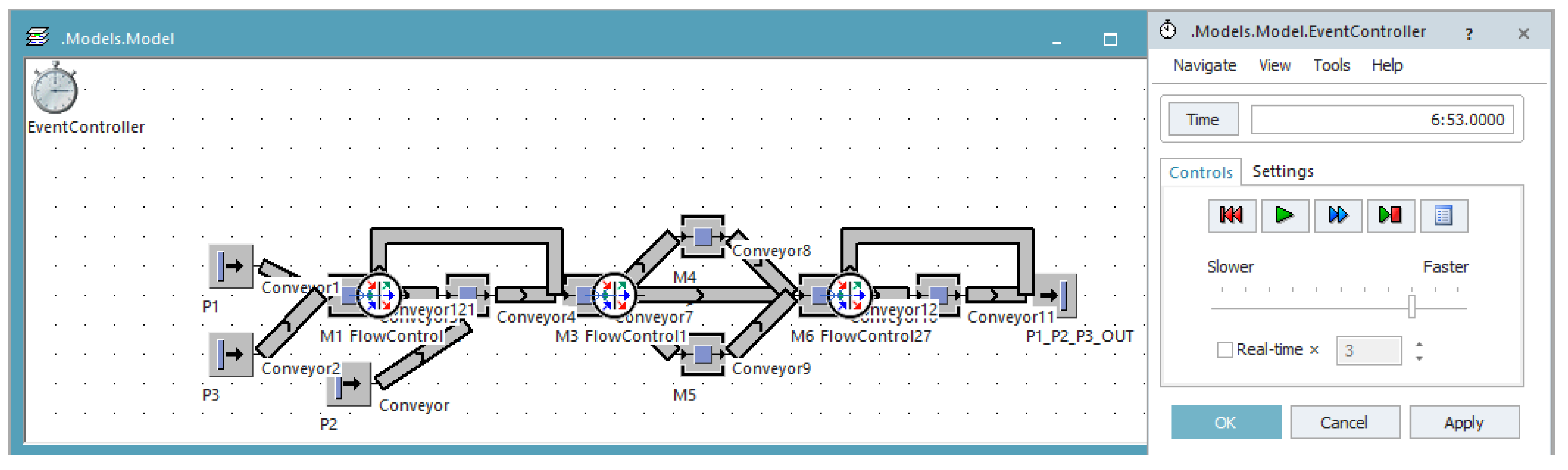
Figure 6.
Theoretical process models.
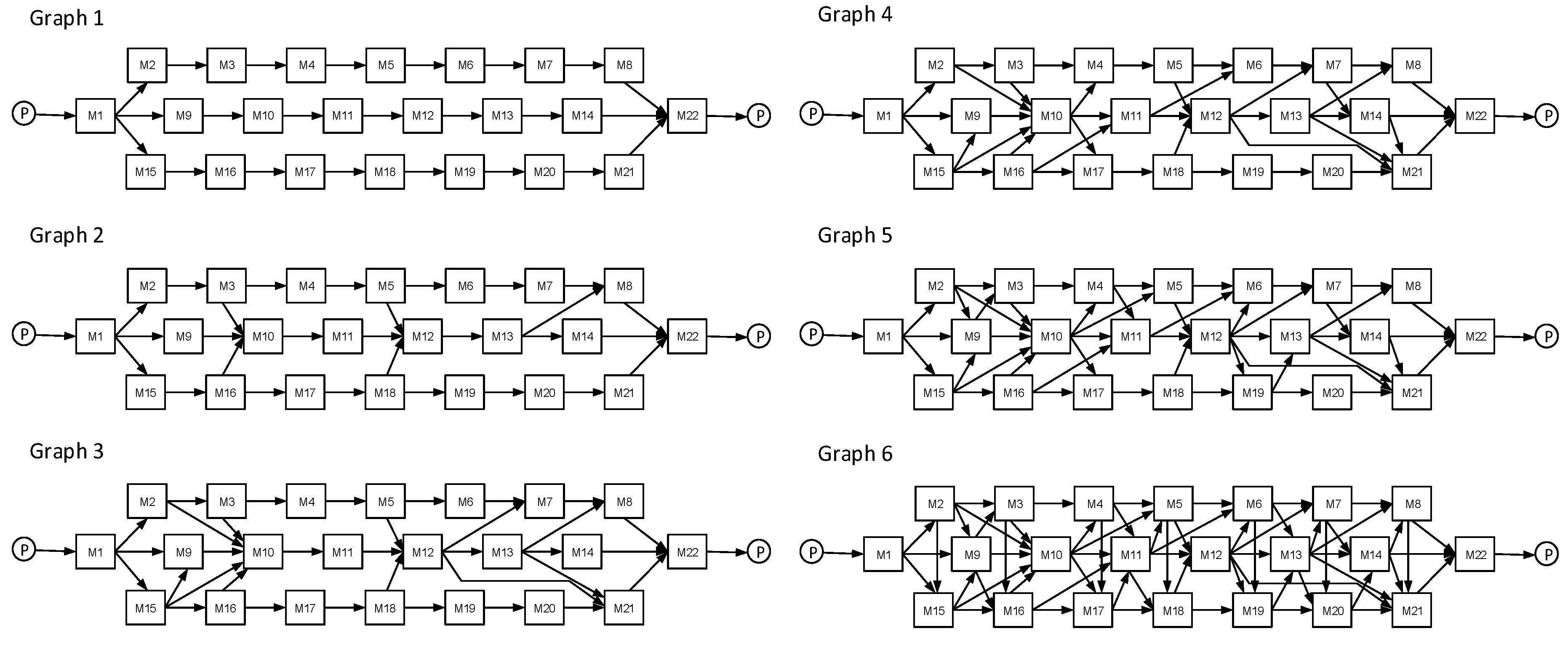
Figure 7.
Process design alternatives A and B.
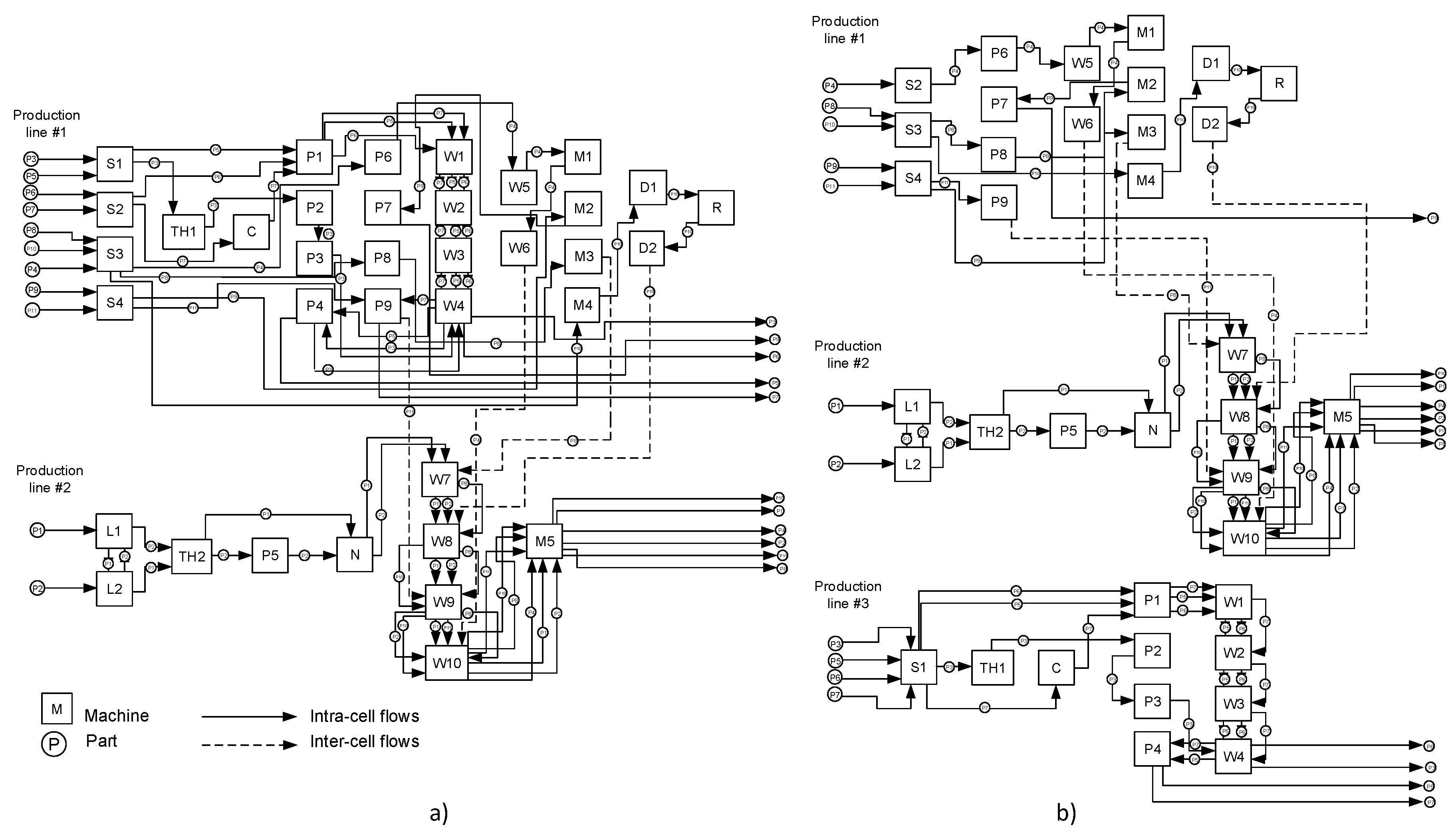
Figure 8.
Process design alternatives C, D and E.


Table 1.
Obtained results for all the six graphs.
| Indicators | Graph 1 | Graph 2 | Graph 3 | Graph 4 | Graph 5 | Graph 6 |
|---|---|---|---|---|---|---|
| M(G) | 0,073 | 0,063 | 0,055 | 0,049 | 0,046 | 0,033 |
| MLT (min) | 109,05 | 109,1167 | 109,117 | 111 | 112 | 114,5 |
| PCI (bits) | 9,15 | 9,72 | 10,13 | 10,5 | 11,16 | 12,5 |
Table 2.
Sequence of machines for five process design alternatives.
| Part number | Sequence of machines with their operational times in seconds |
|---|---|
| P1 | L1(30) - L2(30) - TH2(35) - N(6) - W7 (15) - W8(40) - W9(40) - W10(103) - M5(30) 109,05 |
| P2 | L1(30) - L2(30) - TH2(35) - P5(10) - N(6) - W7(15) - W8(40) - W9(40) - W10(103) - M5(30) |
| P3 | S1(32) - TH1(24) - P2(15) - P3(24) - W4(43) |
| P4 | S2(8) - P6(20) - W5(64) - M1(9) - W6(78) - W10(103) -M5(30) |
| P5 | S1(32) - P1(24) - W1(26) - W2(23) - W3(43) - W4(43) - P4(15) |
| P6 | S1(32) - P1(24) - W1(26) - W2(23) - W3(43) - W4(43) |
| P7 | S1(32) - C(38) - P1(24) - W1(26) - W2(23) - W3(43) - W4(43) - P4(15) |
| P8 | S4(12) - P8(10) - M3(20) - W7(15) - W8(40) - W9(40) - W10(103) - M5(30) |
| P9 | S3(12) - M2(20) - P7(10) |
| P10 | S4(12) - M4(20) - D1(14) - R(12) - D2(14) |
| P11 | S3(12) - P9(10) - W9(40) - W10(103) - M5(30) |
Table 3.
Transport times in seconds for all the three process design alternatives.
| From-to- station | Alt. 1 | Alt. 2 | Alt. 3 | Alt. 4 | Alt. 5 |
|---|---|---|---|---|---|
| W6 - W10 | 53 | 41 | 36 | 46 | 41 |
| P9 – W9 | 57 | 46 | 46 | 50 | 41 |
| D2 – W8 | 35 | 23 | 23 | 23 | 4 |
| M3 – W7 | 37 | 25 | 25 | 25 | 21 |
| N - W7 | - | - | - | - | 20 |
Table 4.
Obtained results for all the five process design alternatives.
| Indicators | Alt. A | Alt. B | Alt. C | Alt. D | Alt. E |
|---|---|---|---|---|---|
| M(G) | 0,00079 | 0,00127 | 0,00126 | 0,00165 | 0,00244 |
| MLT(min) | 13,25 | 13,07 | 13,07 | 13,13 | 12,98 |
| PCI(bits) | 51,7 | 46,8 | 47,8 | 44,4 | 44,08 |
Disclaimer/Publisher’s Note: The statements, opinions and data contained in all publications are solely those of the individual author(s) and contributor(s) and not of MDPI and/or the editor(s). MDPI and/or the editor(s) disclaim responsibility for any injury to people or property resulting from any ideas, methods, instructions or products referred to in the content.ň |
© 2023 by the authors. Licensee MDPI, Basel, Switzerland. This article is an open access article distributed under the terms and conditions of the Creative Commons Attribution (CC BY) license (http://creativecommons.org/licenses/by/4.0/).
Copyright: This open access article is published under a Creative Commons CC BY 4.0 license, which permit the free download, distribution, and reuse, provided that the author and preprint are cited in any reuse.


