
Submitted:
17 May 2023
Posted:
18 May 2023
You are already at the latest version
Abstract
The osseointegration process in and around additively manufactured (AM) lattice structures of a new titanium alloy, Ti–19Nb–14Zr, was evaluated. Three different implants, including lattices with increasing high sidewalls gradually closing them, were designed, manufactured and implanted in the tibia and metatarsal bone of two sheep for twelve weeks. After removal, they were characterized with X-ray computed tomography (XCT). The 3D XCT images were segmented using machine learning. The bone-interface implant (BII) and bone-implant contact (BIC) were studied. The results show that, since AM naturally leads to high roughness surface finish, the wettability of the implant is increased. The new alloy possesses an increased affinity to the bone enhancing the quality of osseointegration. The lattice provides crevices, in which the biological tissue can jump in and cling. The combination of these factors is pushing ossification beyond its natural limits. Therefore, the quality and speed of the ossification and osseointegration in and around these Ti–19Nb–14Zr AM laterally closed lattice implants open the possibility of bone spline key of prostheses. This enables the stabilization of the implant into the bone while keeping the possibility of punctual hooks allowing the implant to be removed more easily if required.
Keywords:
osseointegration
; animal surgery
; implants
; lattices
; titanium alloy
; additive manufacturing (AM)
; X-ray computed tomography (XCT).
1. Introduction
Additive manufacturing (AM) enables the fabrication of lattice structures. Such structures promote bone growth in implantology. This bodes for the stability of the implant, which is a very interesting aspect for the medical sector. Indeed, a better and faster osseointegration of the implant into the human body allow the patient to recover faster. In a previous article [1], we have already demonstrated that the lattice promotes osseointegration implementing the titanium alloy Ti6Al4V grade 23, containing aluminum (Al) and vanadium (V), already widely used for dental and hip implants. This study concerned mainly the conformity of the implants to their computer-aided design (CAD) and powder particle adhesion to the lattices. The bone formation was only qualitatively studied by visual observations on X-ray computed tomography (XCT) images of the implants placed in a sheep for eight weeks.
In the present work, a new-patented titanium alloy for implant [2], called ZTM14N, containing niobium (Nb) and zirconium (Zr) instead of Al and V, was investigated. This material has lower elastic modulus (38 GPa) than other titanium alloys (100 to 130 GPa for TA6V [3]), and contains highly biocompatible materials [4,5,6].
Such properties make the ZTM14N alloy the best alternative material for the medical market. Indeed, a significant stiffness mismatch between the human bone (25-30 GPa) and the implant material causes a stress effect that leads to bone resorption. Bone resorption can be detrimental when the degradation of existing bone predominates over bone formation. Furthermore, release of both V and Al ions from Ti6Al4V, in the human body, might cause long-term health problems, such as peripheral neuropathy, osteomalacia, and Alzheimer’s diseases [7,8].
In addition, the duration of the implantation concerned two sheep and lasted twelve weeks instead of eight weeks in the previous study. This longer residence time is the classical duration fracture consolidation.
The purpose of this new study was twofold. First, the study of the contact between the bone and the implant from two points of view: 1) the bone interface implant (BII), i.e. the interface thickness between bone and implant surfaces, and 2), determined from BII, the bone-implant contact (BIC), i.e. the proportion of the implant surface in contact with bone. Second, the study of the bone progression in depth as a function of the lattice access, as well as a function of bone location into the body (tibia or metatarsal bone).
The histomorphometry of the BIC, i.e. the ratio of bone over metal, is traditionally performed by microscopy on prepared glass slides, and it is by nature 2-dimensional (2D). In this work, the study is performed on XCT images segmented implementing machine learning (ML) algorithms. Thus, the study is performed from 3-dimensional (3D) and statistically sounder (large volumes). But the BII study is performed meticulously on 2D slices that can be extracted in any directions from these 3D images.
The article will address the materials and methods including the implants with a lattice structure design and fabrication in the new titanium alloy using a laser beam powder bed fusion (PBF-LB) AM process; the description of the animal model and sheep surgeries; the details of the implant characterization using an XCT system; the XCT image analysis implementing a machine learning (ML) segmentation, and the procedure used for the evaluations of the osseointegration process (BII, BIC and bone progression in lattice).
Finally, the article will address the results and discussion related to the evaluations of the osseointegration process.
2. Materials and Methods
2.1. Implants
2.1.1. Designs with a lattice structure
To study the bone growth in implants including a lattice structure, three different implants were designed (Figure 1) with the characteristics below:
- ➢
- General shape of the three designs: cylinders with a diameter of 6 mm and a top hexagonal hole concieved to accommodate a holder;
- ➢
-
Differences between the three different designs:
- short side-open cylinder: 5 mm of lattices for 8 mm in total height. The top and bottom of the cylinder are closed by dense surfaces. In this way, the bone penetration is peripherally limited (Figure 1 a);
- side-closed cylinder: 8 mm of lattice for 10 mm in total height The bottom of the cylinder is open. In this way, the bone penetration is bottom limited (Figure 1 b).
- half-side-closed cylinder: 10.4 mm of lattice for 12.4 mm in total. The top and bottom of the cylinder are closed by dense surfaces. In this way, the bone penetration is half peripherally limited (Figure 1 c);
- ➢
- Shape of the elementary cells of the lattice: cubic octahedron (diagonal cell);
- ➢
- Size of the elementary cells of the lattice: 900 µm (octahedron with diagonal cell side of 350 µm) or 1200 µm (octahedron with diagonal cell side of 450 µm);
- ➢
- Number of implants studied: five labelled 1382, 1384, 1385, 1387, and 1386 as targeted in Figure 1.
2.1.2. Manufacturing in a New Titanium Alloy Using a Powder Bed Fusion-Laser Beam (PBF-LB) Process
The implants (Figure 2) were additively manufactured with a laser beam powder bed fusion (PBF-LB) process by Z3Dlab using the patented titanium alloy Ti–19Nb–14Zr (at %), hereinafter ZTM14N [2]. The pre-alloyed powder of Ti–19Nb–14Zr (at %) was produced using powder atomization to get a spherical shape powder. A SLM 125HL (SLM solution) PBF-LB machine, equipped with a 200 W ytterbium fiber laser, was employed. The layer thickness was chosen to be 30 µm and the temperature of the building platform was kept constant at 200°C to minimize residual stresses.
None of these samples underwent heat treatment or polishing. However, the following cleaning protocol was applied:
- 1)
- 60 min in an ultrasound tank with 60°C distilled water without any detergent;
- 2)
- 30 min soaking in Dentasept 3H rapid for decontamination;
- 3)
- Rinsing by ultrasound;
- 4)
- Cleaning with benzalkonium chloride, chloramine T, E.D.T.A betatetrasodium, and isopropylic alcohol;
- 5)
- Drying at DPH21;
- 6)
- Sterilization by surgical autoclave.
At the end, the bulk density and density of the implant were measured with a He-pycnometer and are, respectively, 99.95% ± 0.05 % and 5.54 g/cm3.
2.2. Animal
2.2.1. Animal Model
Two female sheep were involved in this study performed in accordance with good laboratory practices. The sheep were bred by the French National Research Institute for Agriculture, Food and Environment (Institut national de recherche pour l'agriculture, l'alimentation et l'environnement-INRAE). The animal ages were ranging in between five and half, and six years, and their weight were around 55 kg. Tibias and metatarsal bones were used for the inclusion of all the implants. During two days, immediately following implant’s placement surgery, the two sheep were housed in individual pens with eye contact. Then, they were housed in a paddock with a group of sheep until the implants’ removal surgery. In this paddock, the temperature was maintained between 19°C and 22°C, the sheep were exposed to an artificial 12L-12G light cycle, and they were supplied with vegetal bedding, ad libitum hay and water. A daily check of their physical condition was performed throughout the study.
2.2.2. Surgical Steps of the Implant’s Placement
The surgical operations (Figure 3 a) enabling to place and to remove the implants into the sheep have been approved by the French ministry of research after ethical evaluation by the facility ethical committee. These operations were performed by a surgeon assisted by a technician at the biomedical research center of the national veterinary school of Alfort in France (Centre de Recherche BioMedicale -CRBM- de l’Ecole Nationale Vétérinaire d’Alfort). The center has a dedicated operating room for both large and small animals. Prior to the operation, the sheep underwent a complete veterinary examination and then an anesthesia. The anesthetic and analgesic protocol performed by an anesthetist implied the following steps:
- 1)
- Premedication by intravenous injection of a mixture of Ketamine (6 mg/kg) and Diazepam (0.5 mg/kg);
- 2)
- Intubation with an endo-tracheal probe of 9 mm internal diameter;
- 3)
- Connection to respirator with maintenance of anesthesia by inhalation of 2.5 % Isoflurane in an air / oxygen mixture with 60 % O2;
- 4)
- Analgesia: IV injection of Morphine (0.1 mg/kg);
- 5)
- NSAIDs: IM injection of Meloxicam (0.4 mg/kg);
- 6)
- Antibiotic: IM injection of 0.15 ml/kg of PeniDHS (combination of Penicillin and Streptomycin).
After anesthesia, the sheep’s legs were shorn and brushed with chlorhexidine. Then, the cylindrical specimens were placed (Figure 3 c) in a bone cavity, of the tibias and metatarsal bones, previously drilled at the right dimensions (Figure 3 b) by tilting the periosteum, following a strict protocol. Dental implantology equipment was used.
2.2.3. Surgical Steps of the Implant’s Removal
The euthanasia of the sheep, after twelve weeks, was made by premedication by intravenous injection of a mixture of Ketamine (6 mg/kg) and Diazepam (0.5 mg/kg) followed by an injection IV of 20 ml of Pentobarbital 18 %. For the removal of the implants, the surgical site was taken over by the same approach as the placement surgery. A visual inspection of this surgical site was carried out and compared to the site after the implants’ placement (Figure 4). Then the bone parts including the cylindrical specimens were sliced and immediately frozen at -18 °C. Finally, the parts were transferred in dry ice to the BAM in Berlin where they were kept frozen at -18 °C before the XCT characterizations.
2.3. Characterization of the Implant Using an X-ray Computed Tomography (XCT) System
X-ray computed tomography (XCT) imaging was conducted at BAM with an industrial General Electric (GE) phoenix v|tome|x L 300/180 cone beam XCT system. This system includes a 300 kV microfocus X-ray tube as well as a 180 kV high-resolution nanofocus X-ray tube. The entire system is mounted on a granite-base 8-axes manipulator. The 180 kV high-resolution nanofocus X-ray tube was used for the scanning of the implants. This tube includes a transmission target made of tungsten on diamond with a minimum focal spot size of 1 μm. The custom bay system is also equipped with a GE 2048 × 2048 pixels (200 μm pitch) 14-bit amorphous silicon flat panel detector. The acquisitions as well as the reconstruction after the scans were performed with the phoenix datos|x GE software.
A photo of the set-up is shown in Figure 5. The samples were removed from the freezer just before the acquisitions and returned to the freezer immediately after the acquisitions. They were not maintained at -18 ° C during acquisitions. The XCT parameters used are provided in Table 1. No filter was used. A geometrical magnification of 30 was achieved by positioning the samples close to the beam X-ray source (Figure 5 a), giving an effective voxel size of 6.8 μm.
2.4. Analysis of the XCT Images Implementing a Machine Learning (ML) Segmentation
The separation of the metal, bone, pores, osteoid tissue, and metallic grains from each other on the 3D images was carried out with the Ilastik program [9] and two custom in-house 2D UNets [10], forming a three-stage sequential ML process. Ilastik was used to annotate/generate efficiently the training data which were subsequently employed to train the UNets. This approach reduced considerably the time required to annotate the training labels compared to purely manual annotation. In other words, we accelerated the annotation of the required (by the UNets) training labels with the ML capabilities of Ilastik.
Ilastik has been developed by the Ilastik team in Anna Kreshuk's laboratory at the European Molecular Biology Laboratory (EMBL) in Heidelberg (Germany), and uses iterative ML algorithms to segment, classify, track and count the different image areas in 2D images and 3D stacks.
The pixel classification workflow in Ilastik assigns pixels to a group based on pixel/voxel features. These features can be selected by the user from a wide range of operations, for example smoothed pixel/voxel intensity, edge filters and texture descriptors. The user then selects some representative areas in the 3D image stack by color-coding the different areas to be segmented. Based on the image areas assigned to the classes by the user, the system interactively trains a random forest classifier. The predictions in the image data can be previewed so that the training can be improved interactively. The result is a unique classification of each pixel/voxel, into a previously defined class. These classifications can then be extracted.
The main challenge with these XCT datasets is that it is very difficult to distinguish the bone and osteoid phases form each other based solely on grey values, as they appear very similar. The osteoid phase appears typically slightly darker compared to the bone phase due to its lower density. However, the variation of contrast arising from beam hardening within the XCT datasets, can result in certain regions where the bone phase appears darker compared to the osteoid phase located at a different region (i.e. regions in different images within the 3D stack, or different locations within the same image). An example of this is shown in Figure 6. The complete segmentation of the datasets with Ilastik could had been possible, but with a lot more (manual) effort to account for all deviations across all regions. Our three-stage ML segmentation method accelerated the whole process by overcoming the above limitations.
Our training strategy was the following:
Firstly, we conditioned the five XCT datasets (labeled: 1382, 1384, 1385, 1386, and 1387) with a Non-Local-Means (NLM) filter [11] (parameters: sigma = 2, smoothing_factor = 1) to reduce noise. Secondly, we extracted from dataset 1385 eleven random images (4+1 along xy plane, 2 along xz plane, and two along yz plane, (xy, xz, and yz planes as shown in Figure 7). Ilastik was employed to annotate the various phases/labels only within these eleven images (metal, bone, pores, osteoid tissue, and metallic grains) which then served as the training/validation/testing data for the UNets. The extra (+1) image from the xy plane was reserved only for testing the final segmentation accuracy (i.e., training/validation: ten image pairs, testing: one image pair). Thirdly, to increase the number of training/validation data, we randomly mirrored/rotated the ten images to a total of 2000 image pairs (input images and ground truth labels), of which 1800 image pairs (90%) were used as training data, and 200 image pairs (10%) were used as validation data. To improve generalization (i.e. to distinguish the similar bone and osteoid phases better during segmentation), we introduced to the training/validation datasets random brightness and contrast augmentations (+/- 10%) in random order and intensity, moderate random Gaussian noise (0 – 8 in 8-bit grayscale range: 0 – 255), and random Gaussian blur (random sigma: 0 – 1). This approach has been proven by Tsamos et al. [12] to improve considerably the segmentation accuracy of different phases in XCT scans with overlapping grey levels. To further improve the segmentation accuracy, the training of the UNets was undertaken in two stages with a different UNet in each stage. The first UNet was trained to segment the various phases while treating the bone and osteoid phases as a single phase (i.e. 5 phases: metal, pores, metallic grains, bone/osteoid combined, and background). The second UNet was responsible of segmenting only the challenging bone and osteoid phases while considering the rest phases as background (i.e. 3 phases: bone, osteoid, and background). Effectively, the regions in the training/validation image pairs belonging to the metal, pores, and metallic grains phases were nulled (i.e. converted to “black” background) before training the second UNet. Samples of the training/validation/testing data used for the two UNets are illustrated in Figure 7.
The UNets architectures (shown in Figure 8), were designed and trained with Sony’s Neural Network libraries [13] on a workstation equipped with a GeForce RTX 3090 graphics card (Nvidia, Santa Clara, CA, USA), an Intel i7 CPU (Intel, Santa Clara, CA, USA), and 32 GB of memory. The ADAM optimizer [14] was selected as the training algorithm (parameters: initial learning rate/alpha = 10−4, beta1 = 0.9, beta2 = 0.999, updated every iteration), with an input batch size of 8, and random shuffling for the training dataset on each epoch. The learning rate was updated exponentially on every epoch with a learning rate multiplier LRM = 0.95, and we trained for a total of 300 epochs with Categorical Entropy Loss. The decisive (learnable/trainable) parameters within the UNets architectures were adopted from the epoch that minimized the validation error. Based on the reserved testing image, we report a global accuracy Dice score of 85%.
Our forwarding strategy was the following:
We sliced the NLM conditioned XCT datasets/stacks in 2D images along all three planes (i.e. xy, xz, and yz planes) and, for each plane, we applied four rotations (0°, 90°, 180°, and 270°). Thus, this resulted in 12 different sets of images (12 different views). Each set was forwarded through the first (trained) UNet, resulting in 12×5 (5 possible phases for the first UNet) probability map sets. These probability map sets were rotated back to 0° and assembled back into 3D stacks according to the plane direction that were initially sliced, resulting in 12×5 probability map 3D stacks. Finally, the probability stacks were summed together according to their respective phase probability group, resulting in 5 probability stacks for the 5 phases. The final classification (i.e. assigned class/label: metal, pores, metallic grains, bone/osteoid combined, or background), was assigned based on the highest phase probability across all 5 probability stacks for each voxel. Based on this segmentation (i.e. from the first UNet), the grey levels of regions (voxels) in the XCT datasets that were segmented/classified as: metal, pores, and metallic grains were nulled to appear as background. Next, a similar “multi-view” slicing of these datasets was performed before being fed into the second UNet. The assembly and final classification procedure was exactly the same as in the case of the first UNet (but this time with 3 probability stacks for the 3 phases: bone, osteoid, or background). Finally, we maintained the: metal, pores, metallic grains, and background assigned labels from the first UNet segmentation, and the: bone and osteoid labels from the second UNet segmentation to compose the concluding segmentation (Figure 9).
2.5. Evaluations of the Osseointegration Process
2.5.1. Bone-Implant Interface (BII) and Bone-Implant Contact (BIC)
The osseointegration process of titanium (Ti) implants in the body begins with the oxidation of Ti on the implant periphery by biological fluids (blood and lymph). This oxidation results in the formation of a TiO2 layer.
This step is followed by the formation of a calcified (but not ossified) layer, of thickness about a few nanometers. Such calcification occurs by adsorption on the oxidized metal by the mean of calcium (Ca) and phosphate ions present in the blood. This layer has been observed by Nishikawa et al. [15], Gato [16], and Sundell et al. [17].
Then, healing proceeds by the formation of an intermediate osteoid tissue, the woven or fibrous bone, in the empty spaces. Ossification takes place within this tissue. However, there remains an interface, called bone-interface implant (BII), between the metal and the bone. The surgical success of the integration and fixation of an implanted device in a human body depends on the stability of the implant. This stability is determined by the biomechanical properties of this BII. BII is the weakest region in the bone–implant system, and most of the failures occur there. A good quality of osseointegration requires a close contact between the bone and the implant over a significant proportion of the implant surface. The thickness of this BII is an important characteristic of the quality of osseointegration [8,18,19]. A thickness of less than 10 µm is recognized as an indicator of high quality implant [8,12].
The fraction of the implant surface in contact with bone i.e. the ratio of bone over metal in a given direction, is provided by the bone-implant contact (BIC), a metric that quantifies the stability and the durability of the implant. Classically, the BIC is evaluated by histomorphometry. In the present article, it was evaluated from the XCT images segmented by ML. According to Bernhardt et al. [11], in 2012, histomorphometry and 3D XCT provide similar results. For Lyu et al. [20], in 2021, the BICs evaluated from histomorphometric sections and those evaluated from 2D XCT sections also showed a strong correlation. Finally, Hong et al. [21], in 2022, found the same correlation. Thus, the measurements performed on 2D slices extracted from 3D XCT images are therefore justified.
The advantages of evaluating the BIC from XCT images rather than from histomorphometry are: a) the non- invasive character of XCT; b) the ability to perform multiple evaluations on different sections (in histomorphometry, the evaluation is performed on thin layers explicitly fabricated); c) the 3D approach. Thus, the evaluation of osseointegration of implants from XCT images seems relevant.
In the present study, BICs of the side-closed cylinder open at its bottom were evaluated (8 mm of lattice for 10 mm in total) (Figure 1 b). The measurements were performed on 1 mm high sagittal sections (see blue rectangle on Figure 10) corresponding to 150 pixels of 6.8 µm (Figure 11).
More precisely, the sections were located at different angular positions at the cylinder periphery: 0°, 45°, 90° and 135° (Figure 12). On these sections, the number of pixels of osteoid tissue in contact with the metal was counted by visual examination.
2.5.2. Bone Progression in the Lattice Structure
The bone progression was evaluated, from 2D slices and 3D images, at the boundary of the metal, on the three different designed implants: short side-open cylinder, side-closed cylinder, and half-side-closed cylinder. Furthermore, to locate the state of the bone development, sagittal sections were considered.
3. Results and Discussion Related to the Evaluations of the Osseointegration Process
3.1. Visual Inspection before the Implant’s Removal
A high overlap of the metal by the bone after twelve weeks can be observed from Figure 4 (b). According to the surgeon’s experience, this can be attributed to the material’s properties of the new proposed titanium alloy, Ti–19Nb–14Zr, containing Nb and Zr instead of Al and V, and more precisely to the Nb. Indeed, the surgeon who performed the operation did not observe such an overlap with conventional and AM titanium alloys [1].
3.2. BII and BIC
Concerning, the BII distance, 10 µm is used as a limit by Nishikawa et al. [8], Jain et al. [12], and the main implant manufacturers of dental implants. In the present study, 1 pixel corresponds to 6.8 µm, which means that the BII is of 3.3 µm, much less than 10 µm, thus even more favorable.
The BIC evaluations performed on the four sections display in Figure 12 are given in Table 2. An area located close to the external border of the side-closed implant, open at its bottom, was investigated for different angular positions at the cylinder periphery.
Over the 603 pixels corresponding to the cumulative height of the four selected sections on the outer portion of the cylinder, 28 pixels representing bone are not in contact with pixels representing metal, i.e. 4.6 %. The contact between the bone and the metal, related to the BIC, is therefore 95.4 %. Such high level of osseointegration promises the highest stability and duration of the implant in the bone. Indeed, classically BICs ranging in between 50 % and 80 % are considered to be favorable scores [22].
A similar count was also performed on the same sections, but on an area located close to the internal border. In this case, the analysis was conducted in the lattice region, of the side-closed implant, open at its bottom, for different angular positions at the cylinder periphery. The results are given in Table 3. Out of the 653 pixels considered, 47 did not show bone/implant contact, a rate of 7.1 %. The difference of the BIC between the internal and external borders of the implant mainly originates from one of the four considered sections, the one located at 90°.
The low thickness of the BII and the importance of the BIC may induce stress concentration at the bone-implant junction if there is a high stiffness difference between the bone and the implant. However, in the present study, the smaller difference between the Young's modulus, i.e. the metric representing the stiffness, of the cortical bone (25-30 GPa) and the new used alloy (38 GPa) has reduced the effective stress compare to other commonly used materials.
3.3. Bone Progression in Lattice Structures
First of all, the bone progression was examined as a function of the location of the implants in the sheep body, i.e. the bone progression in the metatarsal bone was compared to that in the tibia (Figure 13). The percentage of bone (dark blue in Figure 13) and of osteoid tissue (light blue in Figure 13), within the lattice, are, respectively, 20.5 % and 8.8 % for the metatarsal bone, and 26.6 % and 3.9 % for the tibia, for the same sheep. Therefore, it seems that the bone progression is more accentuated in the tibia than in the metatarsal bone. This result confirms that the vascularization, one of the four processes that comes into play in the implant stabilization, is better in the tibia than in the metatarsal bone.
Then, the bone progression was examined as a function of the type of designs of the implants (Figure 14), as a function of the depths in the implants (Figure 15), and as a function of the lattice cell sizes (Figure 16). At 5 mm depth, the bone formation is almost complete for 1200 µm lattice cell size, whatever the implant’s design (Figure 14 b and c, and Figure 15 a and b). At 8 mm, the bone creation is not complete when the cylinder is laterally closed on all its height, for 1200 µm lattice cell size (compare Figure 15 b with Figure 15 c). For 900 µm lattice cell size, the bone creation exists but seems incomplete (Figure 14 c, and Figure 16). However, it is not possible to conclude from this study whether the size of the lattice cell or its location in the sheep's body is the cause for this incomplete ossification.
4. Conclusions
Additive manufacturing naturally leads to a high roughness surface finish. This roughness has a positive effect, as it increases the wettability of the implant. Furthermore, the new proposed titanium alloy, Ti–19Nb–14Zr, has an increased affinity to the bone, which enhances the quality of osseointegration. At last, the lattice provides crevices in which the biological tissue can jump in and cling. The combination of these factors is pushing ossification beyond its natural limits.
In France, in 2017, 19,000 patients had to undergo further surgery for unsealing of their prosthesis. Thus, the stabilization of hip prosthesis requires to be increased, but in anticipation of the need of its removal, the procedure must be simplified by bone spline key that can be easily cut for prosthesis removal. Bone spline key has been already investigated in dental implants by tunnelling their apex into the bone (e.g. Paragon implant). But, the insufficient ossification of this transfixing cavity has led to a disaffection for this technique. However, the type of laterally closed lattice structures described in this article allows this technique to be reconsidered.
The quality and speed of the ossification and osseointegration in and around these new titanium alloy, Ti–19Nb–14Zr, additively manufactured laterally closed lattice implants open the possibility of bone spline key of prostheses that enable the stabilization of the implant into the bone while keeping the possibility of punctual hooks allowing the implant to be removed more easily if required.
Author Contributions
Conceptualization, Anne-Françoise Obaton, Jacques Fain and Madjid Djemaï; Formal analysis, Anne-Françoise Obaton, Jacques Fain, Dietmar Meinel and Athanasios Tsamos; Funding acquisition, Anne-Françoise Obaton, Jacques Fain and Madjid Djemaï; Investigation, Anne-Françoise Obaton, Jacques Fain, Dietmar Meinel and Athanasios Tsamos; Methodology, Anne-Françoise Obaton, Jacques Fain, Dietmar Meinel, Fabien Léonard, Benoît Lecuelle and Madjid Djemaï; Project administration, Anne-Françoise Obaton and Jacques Fain; Resources, Dietmar Meinel and Fabien Léonard; Software, Dietmar Meinel and Athanasios Tsamos; Supervision, Anne-Françoise Obaton and Jacques Fain; Validation, Anne-Françoise Obaton, Jacques Fain, Dietmar Meinel and Athanasios Tsamos; Visualization, Anne-Françoise Obaton and Jacques Fain; Writing – original draft, Anne-Françoise Obaton and Jacques Fain; Writing – review & editing, Anne-Françoise Obaton and Jacques Fain.
Funding
This research did not receive any specific grant from funding agencies in the public, commercial, or not-for-profit sectors.
Institutional Review Board Statement
The surgical operations enabling to place and to remove the implants into the sheep have been approved by the French ministry of research after ethical evaluation by the facility ethical committee.
Acknowledgments
The authors warmly thank Dr. Jean-Charles Giunta, buccal surgeon, with whom Jacques Fain performed the surgical operations and who generously lent his dental implantology equipment.
Conflicts of Interest
The authors declare no conflict of interest.
References
- Obaton, A-F.; Fain, J.; Djemaï, M.; Meinel, D. ; Léonard, F. ; Mahé, E.; Lécuelle, B.; Fouchet, J-J.; Bruno, G. In vivo XCT bone characterization of lattice structured implants fabricated by additive manufacturing: a case report. Heliyon 2017, 3. [CrossRef]
- Djemai, A.; Fouchet, J-J. Process for manufacturing a titanium niobium zirconium (tnz) beta-alloy with a very low modulus of elasticity for biomedical applications and method for productive same by additive manufacturing, WO2017137671A1, WIPO (PCT) Publication 2017-08-17 Worldwide applications 2016*FR US KR EP WO.
- Boyer, R.; Collings, E.W.; Welsch, G. Materials Properties Handbook: Titanium Alloys, USA, 1994.
- Lee, D.-G.; Mi, X.; Kwan Eom, T.; Lee, Y. Bio-Compatible Properties of Ti–Nb–Zr Titanium Alloy with Extra Low Modulus. J. Biomimetics, Biomater. Biomed. Eng. 2016, 6, 798–801. [CrossRef]
- Kurtz, M.; Wessinger, A.; Mace, A.; Moreno-Reyes, A.; Gilbert, J. Corrosion Resistance of Additively Manufactured Titanium Alloys in Physiological and Inflammatory-Simulating Environments: Ti-6al-4v Versus Ti-29nb-21zr. [CrossRef]
- Kurtz, M.; Wessinger, A.; Mace, A.; Moreno-Reyes, A.; Gilbert, J. Additively manufactured Ti-29 Nb-21Zr shows improved oxide polarization resistance versus Ti-6Al-4V in inflammatory stimulating solution. J Biomed Mater Res. 2023, 1-16. [CrossRef]
- Walker, P.R.; LeBlanc, J.; Sikorska, M. Effects of aluminum and other cations on the structure of brain and liver chromatin. Biochemistry. 1989, 28, 3911–3915. [CrossRef]
- Rao, S.; Ushida, T.; Tateishi, T.; Okazaki, Y.; Asao, S. Effect of Ti, Al, and V ions on the relative growth rate of fibroblasts (L929) and osteoblasts (MC3T3-E1) cells. Biomed Mater Eng. 1996, 6(2), 79–86. [CrossRef]
- Berg, S.; et al. Ilastik: Interactive machine learning for (bio)image analysis. Nature methods 2019, 16(12), 1226–1232. [CrossRef]
- Ronneberger, O.; Fischer, P.; Brox, T. U-Net: Convolutional networks for biomedical image segmentation, Lecture Notes in Computer Science. Cham: Springer International Publishing 2015, 9351, 234–241. [CrossRef]
- Buades, A. B.; Coll, J.-M.; Morel, A. Non-Local Algorithm for Image Denoising, IEEE Computer Society Conference on Computer Vision and Pattern Recognition (CVPR’05) 2005, 2, 60–65.
- Tsamos A.; Evsevleev S.; Fioresi R.; Faglioni F.; Bruno G. Synthetic data generation for automatic segmentation of X-ray computed tomography reconstructions of complex microstructures. J. Imaging 2023, 9(2), 22. [CrossRef]
- 13. Neural Network Libraries. An Open-Source Software to Make Research, Development and Implementation of Neural Network More Efficient. Sony Corp. https://nnabla.org/.
- Kingma, D. P.; Ba J. Adam: A method for stochastic optimization, ICLR 2015. https://www.semanticscholar.org/paper/a6cb366736791bcccc5c8639de5a8f9636bf87e8.
- Nishikawa, T.; Masuno, K.; Mori, M.; Tajine, Y.; Kakudo, K.; Tanaka, A. Calcification at the interface between titanium implants and bone observation with confocal laser scanning microscopy. J Oral Implantol. 2006, 32(5), 211-217. [CrossRef]
- Goto, T. Ostéointégration and dentals implants. Clin Calcium 2014, 24 (2), 265-71. https://pubmed.ncbi.nlm.nih.gov/24473360/.
- Sundell, G.; Dahlin, C.; Andersson, M.; Thuvander, M. The bone implant interface of dentals implants in humans on the atomic scale. Acta Biomater 2017, 48, 445-450. [CrossRef]
- Bernhardt, R.; Kublisch, E.; Schultz, M-C.; Eckelt, U. Stadlinger, B. Comparison of bone-implant contact and bone-implant volume between 2D-histological sections and 3D-SRµCT slices. Eur Cell Mater. 2012, 23, 237-247. [CrossRef]
- Jain, R.; Kapour, D. The dynamic interface: a review. J Int Soc Prev Community Dent 2015, 5 (5), 354-58. [CrossRef]
- 20. Lyu, H-Z.; Lee, J. H. Correlation between two-dimensional micro-CT and histomorphometry for assessment of the implant osseointegration in rabbit tibia model. Biomater Res. 2011, 25, 11. [CrossRef]
- 21. Hong, J-M.; Kim, H-G.; Luke Yeo, I-S. Comparison of three-dimensional digital analysis and the two-dimensional histomorphometric analysis of the bone-implant interface. Plos one 2022, 17(10):e276269. [CrossRef]
- Lian, Z.; Guan, H.; Ivanovski, S.; Loo, Y-C.; Johnson, N-W.; Zhang, H. Effect of bone to implant percentage on bone remodeling surrounding a dental implant. Int J Oral Maxillofac Surg. 2010, 39(7), 690-8. [CrossRef]
Figure 1.
The three different designs of the implants with a lattice structure (“meta” stands for metatarsal bone).
Figure 1.
The three different designs of the implants with a lattice structure (“meta” stands for metatarsal bone).
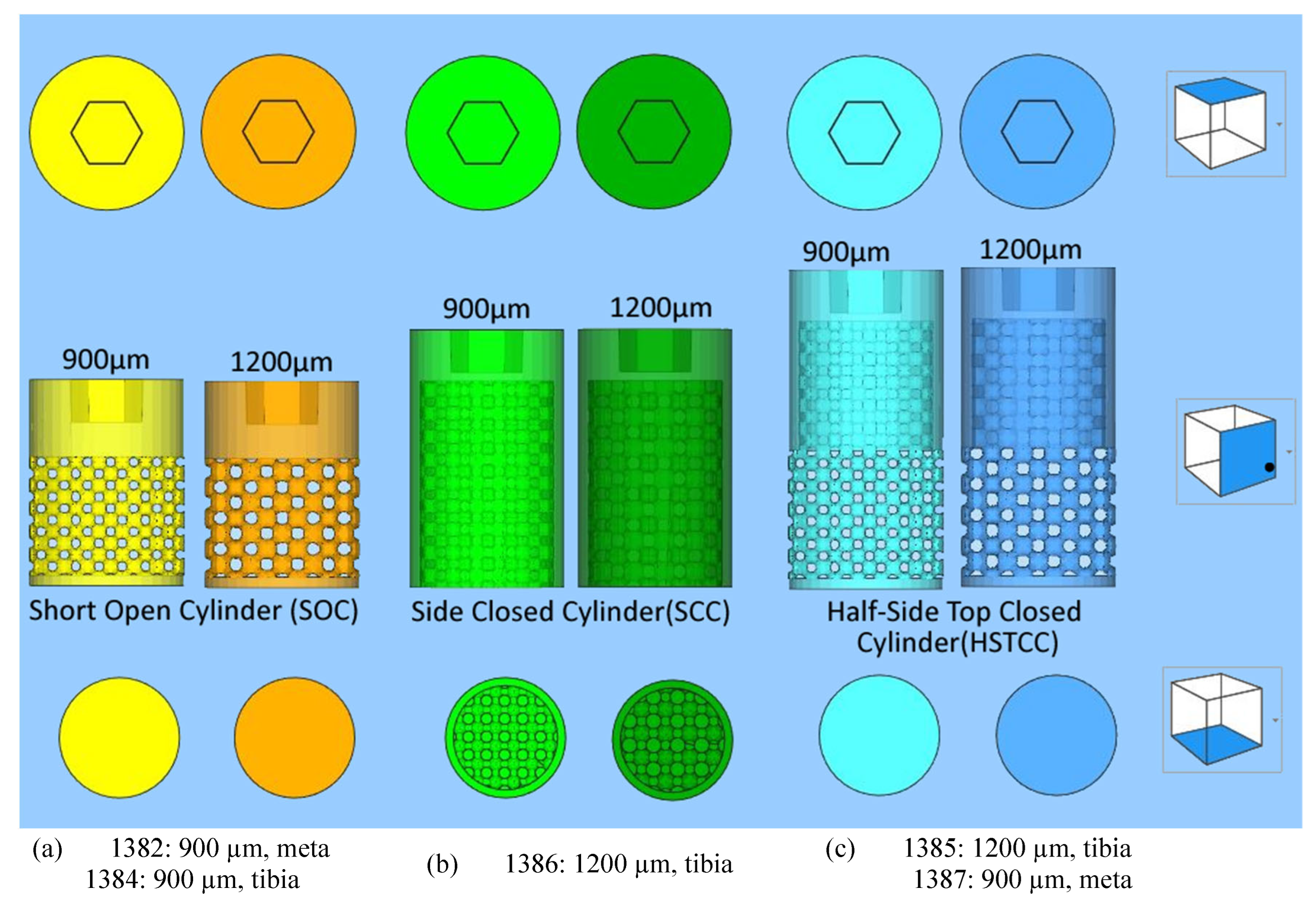
Figure 2.
Titanium alloy manufactured implants with a lattice structure (three different designs).
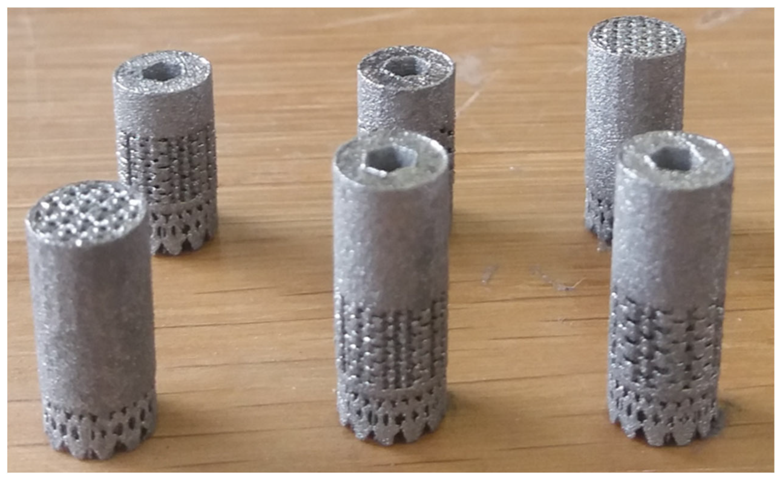
Figure 3.
Surgical steps of the implant’s placement.
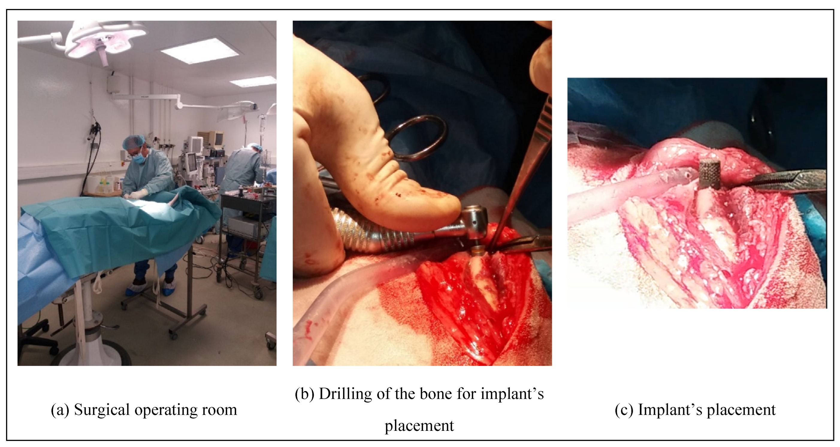
Figure 4.
Comparison of the surgical sites, a) at the end of implant’s placement, b) before implant’s removal, after twelve weeks.
Figure 4.
Comparison of the surgical sites, a) at the end of implant’s placement, b) before implant’s removal, after twelve weeks.

Figure 5.
Implant’s photographs after removal from the sheep and machined for XCT characterization.
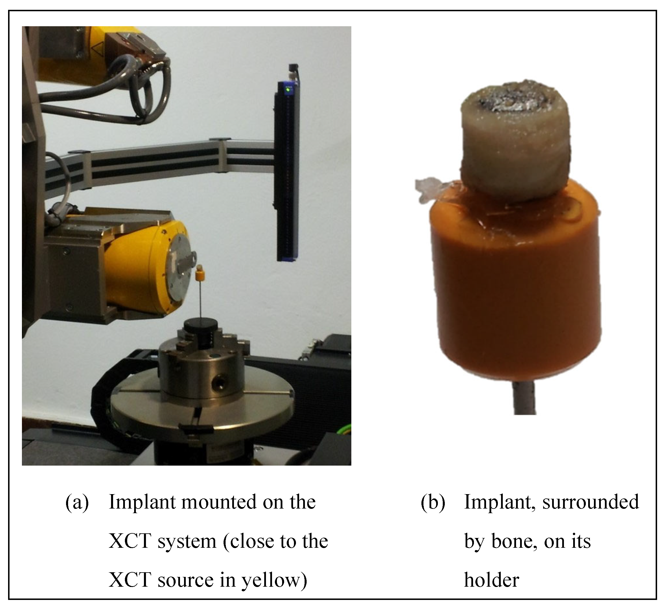
Figure 6.
Bone and osteoid tissue sharing the exact same XCT grey levels at different locations within the same dataset due to beam hardening.
Figure 6.
Bone and osteoid tissue sharing the exact same XCT grey levels at different locations within the same dataset due to beam hardening.
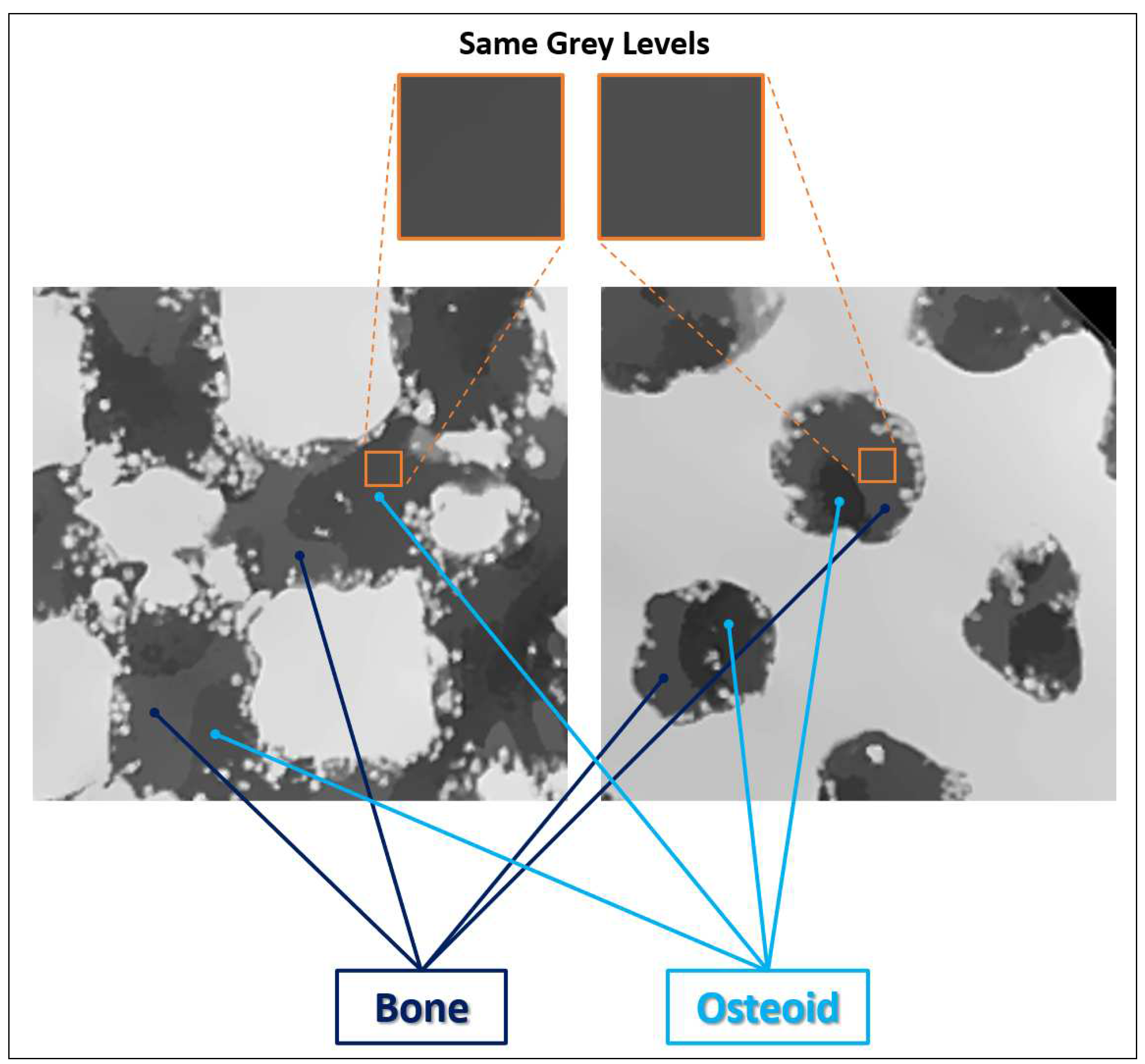
Figure 7.
Training/validation/testing data for the two UNets. Labels: Bone (dark blue), osteoid tissue (light blue), bone and osteoid combined (magenta), pores (red), metal (yellow), metallic grains (green), background (black).
Figure 7.
Training/validation/testing data for the two UNets. Labels: Bone (dark blue), osteoid tissue (light blue), bone and osteoid combined (magenta), pores (red), metal (yellow), metallic grains (green), background (black).
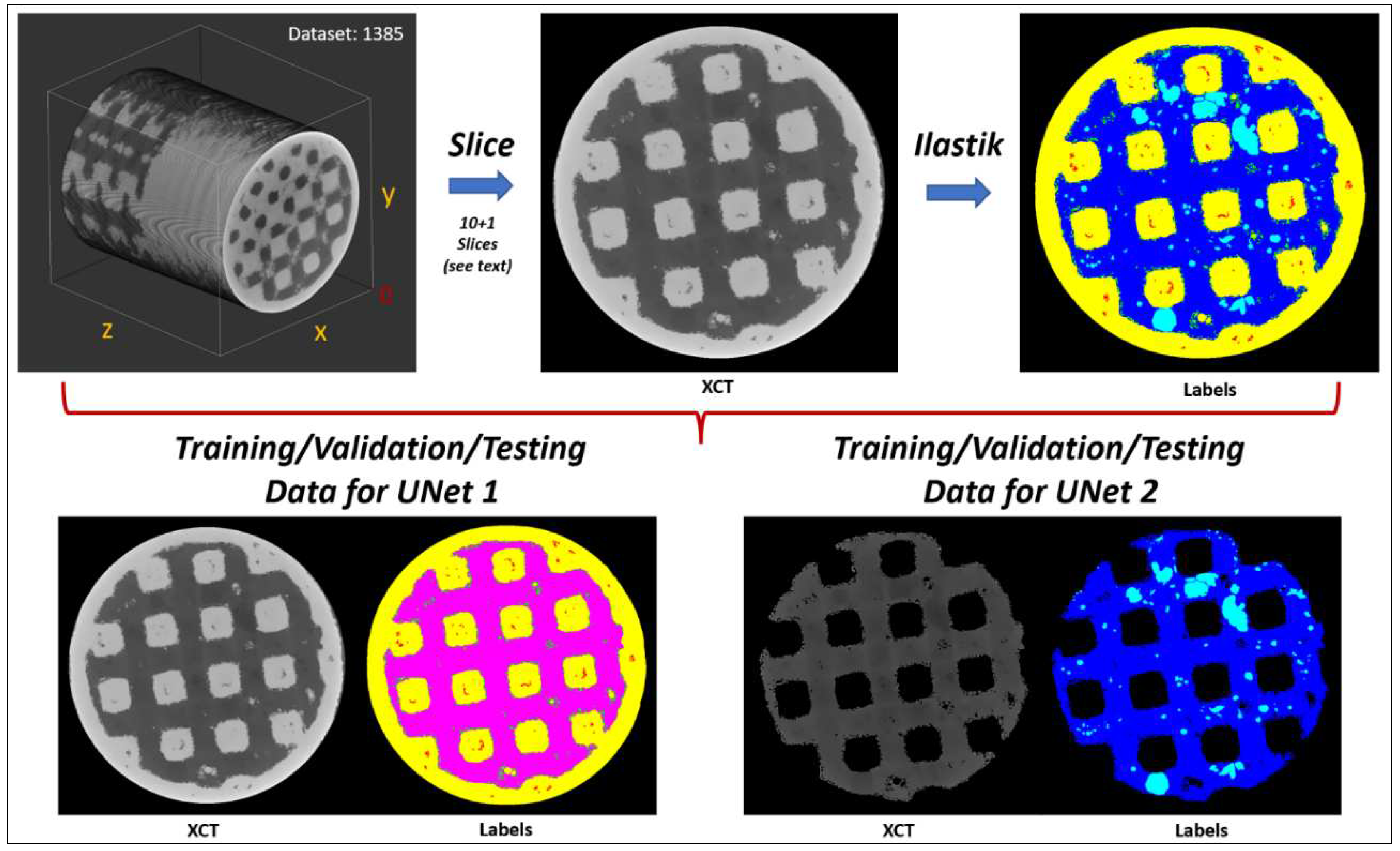
Figure 8.
The two in-house UNet architectures employed for the segmentation.
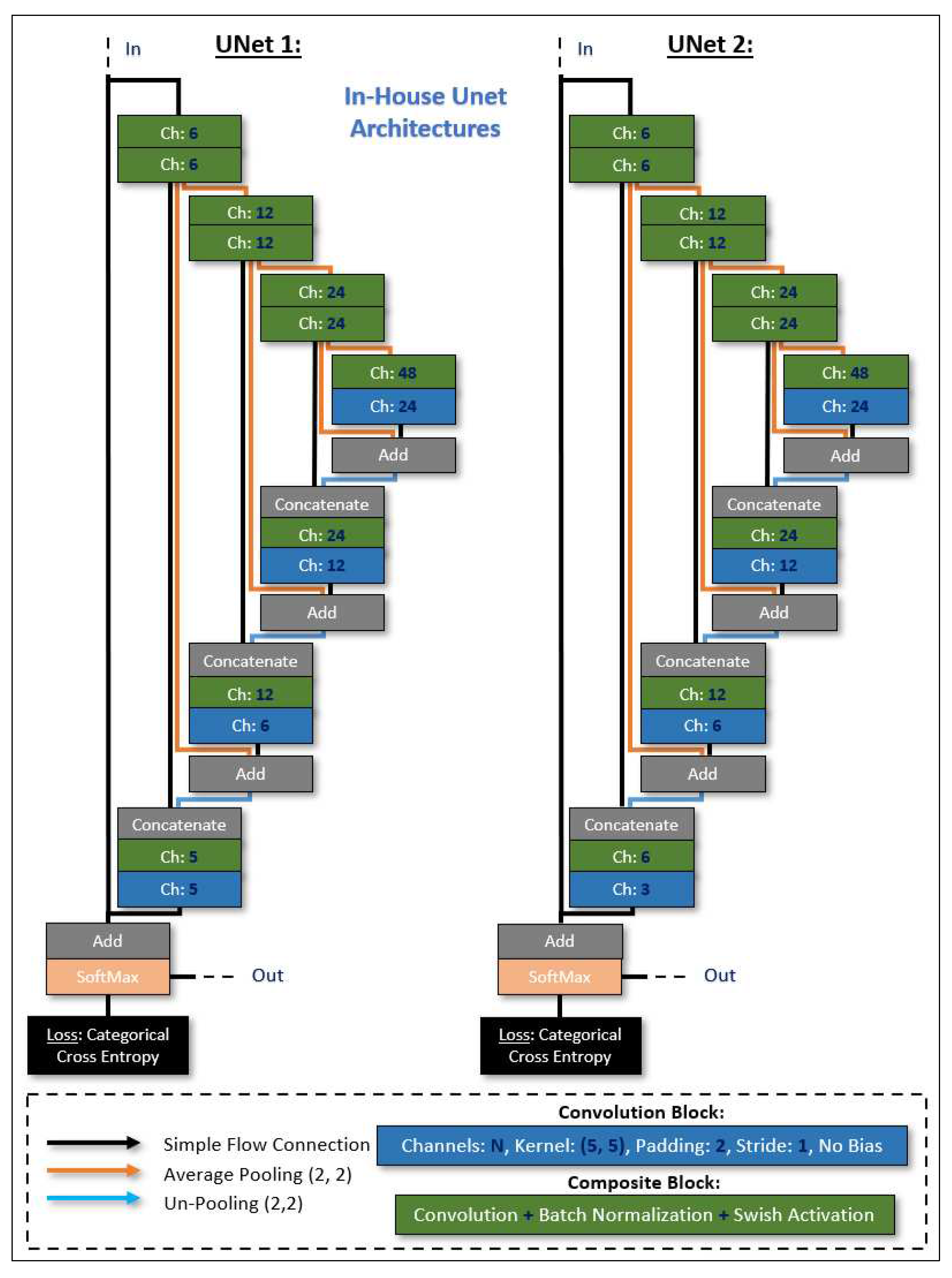
Figure 9.
Implant’s 3D XCT image segmentation performed by the Ilastik program implementing machine learning (ML) algorithms.
Figure 9.
Implant’s 3D XCT image segmentation performed by the Ilastik program implementing machine learning (ML) algorithms.
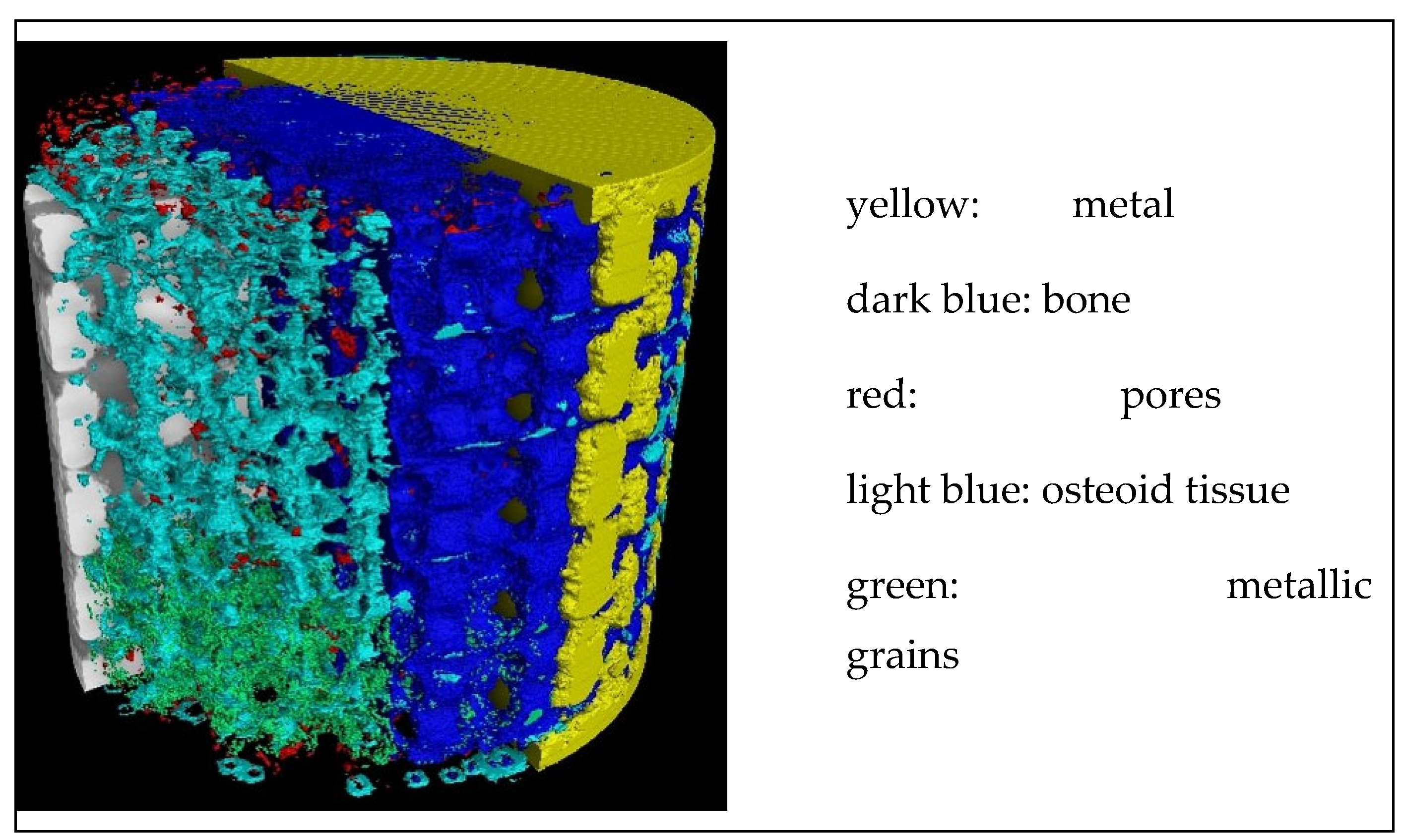
Figure 10.
2D XCT sagittal slice of the side-closed implant, open at its bottom, labelled 1386. The blue rectangle is indicating the sections where the BICs were evaluated.
Figure 10.
2D XCT sagittal slice of the side-closed implant, open at its bottom, labelled 1386. The blue rectangle is indicating the sections where the BICs were evaluated.
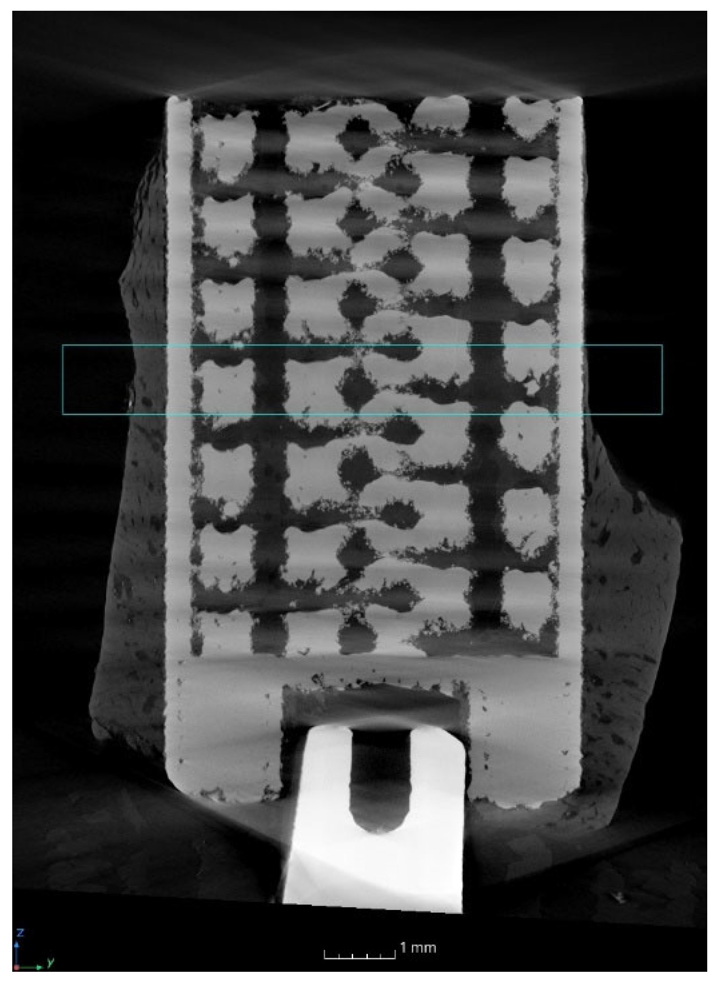
Figure 11.
Greyscale, as well as colored, ML segmented 2D XCT slices of the side-closed implant (labelled 1386), open at its bottom. The inserts are indicating the location where the BICs were measured.
Figure 11.
Greyscale, as well as colored, ML segmented 2D XCT slices of the side-closed implant (labelled 1386), open at its bottom. The inserts are indicating the location where the BICs were measured.
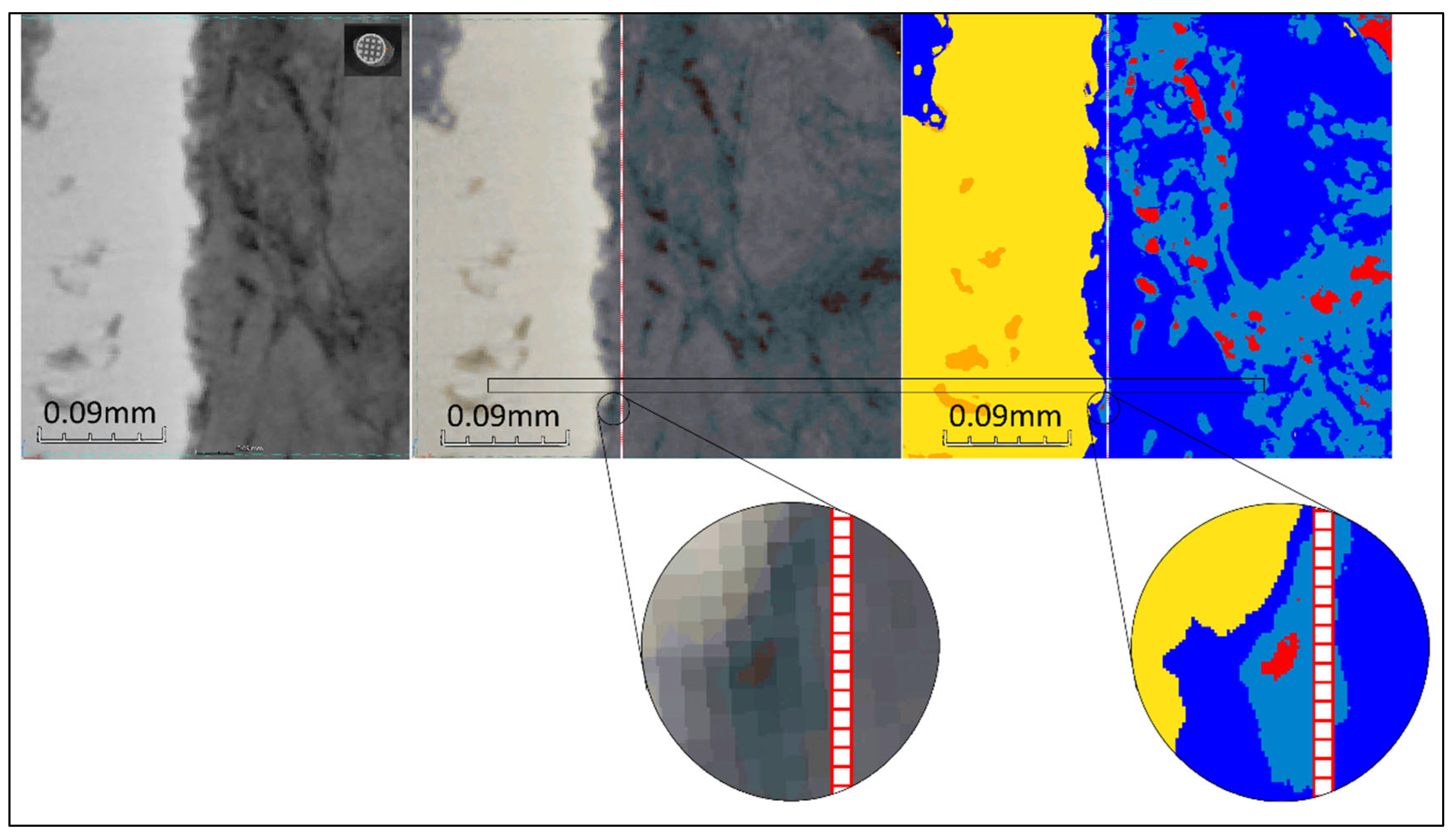
Figure 12.
ML segmented 2D XCT image sections, located at different angular positions at the cylinder periphery, used to evaluate the BICs of the side-closed implant, open at its bottom, labelled 1386.
Figure 12.
ML segmented 2D XCT image sections, located at different angular positions at the cylinder periphery, used to evaluate the BICs of the side-closed implant, open at its bottom, labelled 1386.
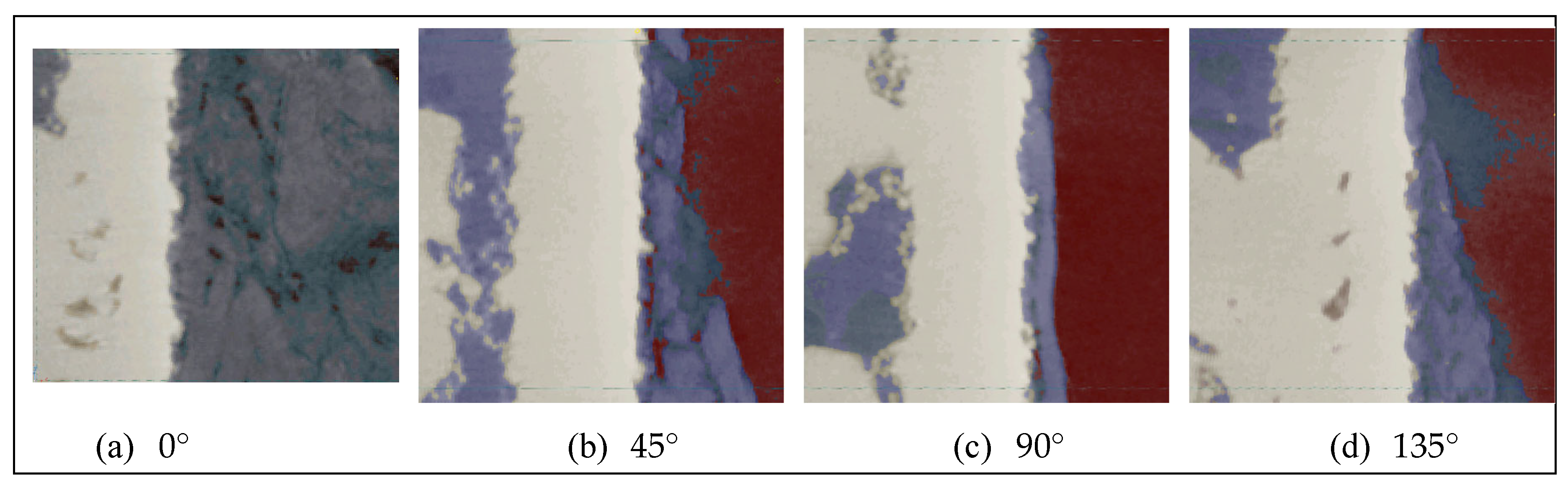
Figure 13.
2D XCT images of implant horizontal and sagittal slices showing the proportion of bone (in dark blue) within the implant (in yellow) compared to other areas (osteoid tissue is in light blue and metallic grains are in green), in the metatarsal bone and tibia.
Figure 13.
2D XCT images of implant horizontal and sagittal slices showing the proportion of bone (in dark blue) within the implant (in yellow) compared to other areas (osteoid tissue is in light blue and metallic grains are in green), in the metatarsal bone and tibia.
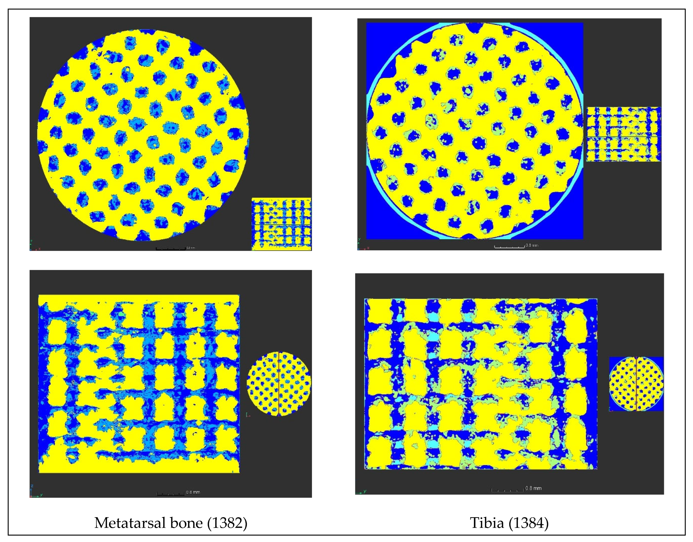
Figure 14.
Bone progression in the three types of designs of the implants: a) side-open cylinder, b) half-side-closed cylinder, and c) side-closed cylinder.
Figure 14.
Bone progression in the three types of designs of the implants: a) side-open cylinder, b) half-side-closed cylinder, and c) side-closed cylinder.
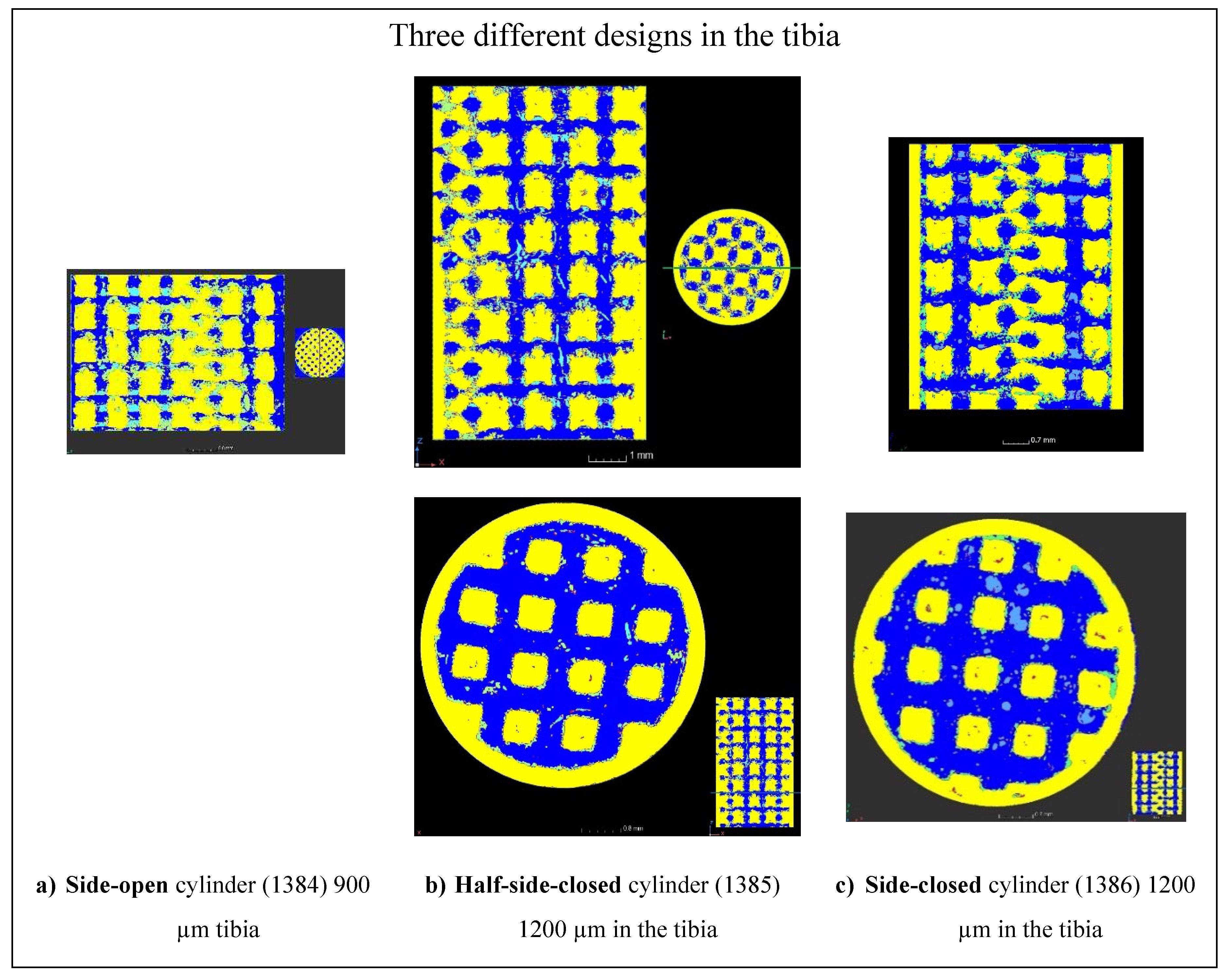
Figure 15.
Bone progression at two different depths in the same implant (Depth 1 = 5 mm and Depth 2 = 8 mm).
Figure 15.
Bone progression at two different depths in the same implant (Depth 1 = 5 mm and Depth 2 = 8 mm).
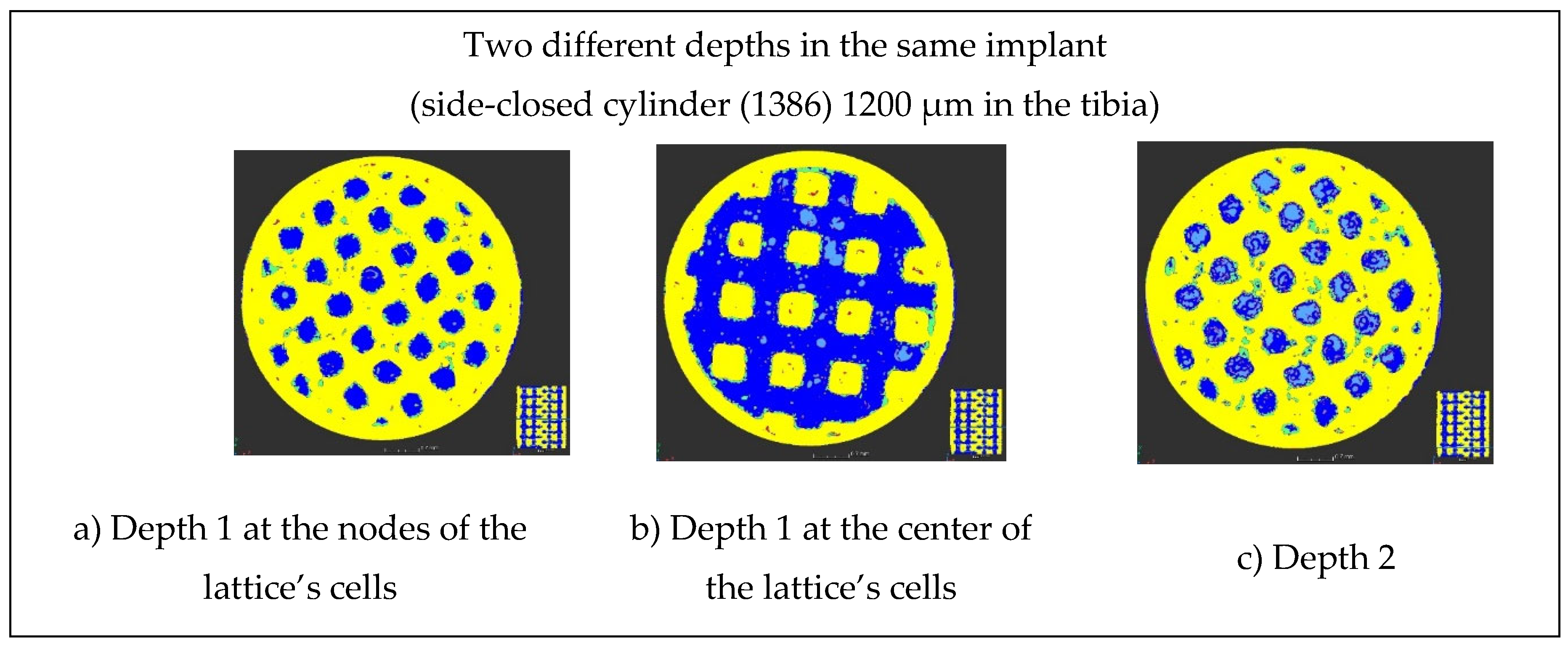
Figure 16.
Bone progression for two different lattice cell' sizes of the same implant design.
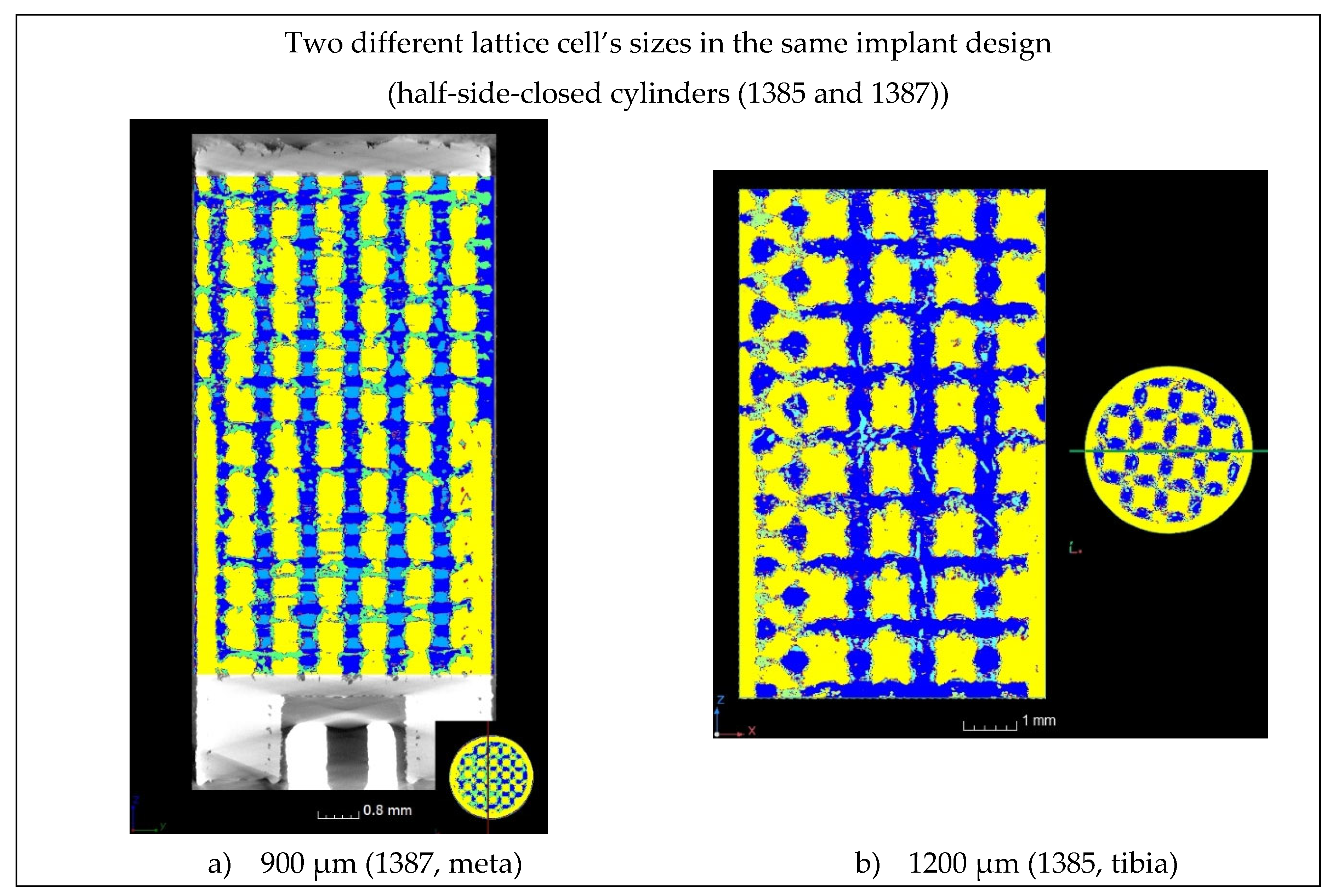

Table 1.
XCT acquisition parameters used for the implant characterizations.
| Accelerating voltage (kV) | Current (µA) | Number of projection | Exposure time per projection (ms) | Number of projection averaged | Scan duration (h) | Voxel size (µm) |
| 120 | 120 | 3142 | 1000 | 2 | 2 | 6.8 |
Table 2.
BIC evaluations performed on an area located close to the external border of the side-closed implant, open at its bottom, labelled 1386, for different angular positions at the cylinder periphery.
Table 2.
BIC evaluations performed on an area located close to the external border of the side-closed implant, open at its bottom, labelled 1386, for different angular positions at the cylinder periphery.
| Angular position around the cylinder | 0° | 45° | 90° | 135° | total |
| Number of pixel in the selected image area | 148 | 151 | 150 | 154 | 603 |
| Number of pixels for which bone and metal have no contact | 1 | 5 | 17 | 5 | 28 |
| % of pixels free of bone or metal | 0.6 | 3.3 | 11.3 | 3.2 | 4.6 |
| ²BIC (%) | 99.4 | 96.7 | 88.7 | 96.8 | 95.4 |
Table 3.
BIC evaluations performed on an area located close to the internal border, in the lattice region, of the side-closed implant, open at its bottom, labelled 1386, for different angular positions at the cylinder periphery.
Table 3.
BIC evaluations performed on an area located close to the internal border, in the lattice region, of the side-closed implant, open at its bottom, labelled 1386, for different angular positions at the cylinder periphery.
| Angular position around the cylinder | 0° | 45° | 90° | 135° | total |
| Number of pixel in the selected image area | 38 | 300 | 254 | 61 | 653 |
| Number of pixels for which bone and metal have no contact | 0 | 0 | 47 | 0 | 47 |
| % of pixels free of bone or metal | 0 | 18,5 | 0 | 0 | 7.2 |
| BIC (%) | 100 | 81.5 | 100 | 100 | 92.8 |
Disclaimer/Publisher’s Note: The statements, opinions and data contained in all publications are solely those of the individual author(s) and contributor(s) and not of MDPI and/or the editor(s). MDPI and/or the editor(s) disclaim responsibility for any injury to people or property resulting from any ideas, methods, instructions or products referred to in the content. |
© 2023 by the authors. Licensee MDPI, Basel, Switzerland. This article is an open access article distributed under the terms and conditions of the Creative Commons Attribution (CC BY) license (http://creativecommons.org/licenses/by/4.0/).
Copyright: This open access article is published under a Creative Commons CC BY 4.0 license, which permit the free download, distribution, and reuse, provided that the author and preprint are cited in any reuse.


