
Submitted:
15 May 2023
Posted:
15 May 2023
You are already at the latest version
Abstract
Due to the numerous heat sources in electronic equipment, the periodic nature of stream-wise flow occurs in a cooling channel so often, necessitating the development of an effective technique to improve the heat-cooling convection in such a situation. This paper investigates thermal convection enhancement in a heated-block duct through the periodic boundary conditions using the element-by-element (EBE) treatment in a semi-implicit projection finite element method (FEM) through preconditioned conjugate gradient (PCG) solver. This paper used the time-mean Nusselt number ratio, friction factor, and thermal performance to study how installing rectangular cylinders in the channel works with periodic boundary conditions varying Reynolds numbers (100, 175, and 250). The outcomes show that the rectangular cylinders installed stream-wise above an upstream block promote thermal convection in the heated-block duct. However, increasing the number of rectangular cylinders can raise friction factor. As a result, the case for periodic boundary conditions with a rectangular cylinder above every two blocks has the best thermal performance.
Keywords:
heat transfer enhancement
; heated-block channel
; mounting rectangular cylinders
; periodic boundary conditions
1. Introduction
In recent decade years, the computer and semiconductor industry's technologies have advanced by leaps and bounds. This fact enforces the numerical computational capability in different thermal convection investigations concerning various practical problems.
The finite element approach has been one of the most significant engineering computational methodologies for complicated linear and nonlinear problems in heat transfer research. Among different finite-element methods, they have two drawbacks: first, they demand a higher matrix stock, and second, they use more CPU memory when solving complicated problems.
Hughes et al. [1] were the first to calculate heat conduction problems using the early version of the EBE plus implicit technique. Hughes et al. [2] and Ortiz et al. [3] employed element by element (EBE) method to solve computational structural issues and integrated these early EBE techniques with "Marchuk-type" iterative computing techniques. To speed up the convergence of iterative solutions, Winget [4] and Hughes et al. [5,6] combined EBE with "preconditioned conjugate gradients (PCG)," referring to these as "Crout types." The "Crout type," used by Levit [7], raised the computational order of EBE to the N order. Carey [8] altered the EBE matrix composition to take the form of a parallel processor; however, the analysis was only for structural issues. Wathen [9] increased the practical computational capability of EBE by expanding its usable dimension from 1-D to 2-D and 3-D. Erhel et al. [10] applied the preconditioned methodology, iterative products, and the EBE calculation method to solve 2-D and 3-D vector problems. Additionally, Papadrakakis et al. [11] used a global matrix pattern to accelerate the convergence rate when they analyzed the usage of the preconditioned methodology in the computation method of EBE. Mizukami [12] chose several large-range flow fields as calculation models, applied the Penalty and Uzawa methodology through a pressure-implicit and velocity-explicit algorithm, and combined the equations in the flow field. He then used the EBE-CG calculation matrix to demonstrate that the latter got less numerical storage and CPU time for calculating large-scale flow fields. EBE was used by Li et al. [13] and Sunmonu [14] to shrink the matrix, speeding up the computer's calculation time. Reddy [15] calculated the flow issue of viscous incompressible fluids by combining two iteration methods (GMRES and ORTHOMIN) with the Multigrid method, using the EBE numerical architecture to reduce the number of convergence during computation.
Through parallel computing and EBE computational fluid dynamics, Nakabayashi et al. [16] were also the first to apply the addition type of EBE to compute fluid flow. He also incorporated the conjugate gradient method to speed convergence, which has the same performance for lowering the need for numerical storage and CPU temporary memory. One of the effective numerical solutions to the problem of heat flow in the unstable state and incompressibility was the semi-implicit projection scheme based on the projection technique [17,18]. As a general rule, the projected finite element method (the semi-hidden finite element method) offers an advantage over the traditional finite-element approach with less computer storage space and less CPU time to compute. Thomas et al. [19] used an element-by-element algorithm to solve incompressible flow inside a cap-pushed square chamber and transient flow over a round cylinder. Their results proved that the correctness of the algorithm was excellent.
On the other hand, a periodic boundary condition of stream-wise flow occurs so often in the heat exchange systems, such as heat exchangers, solar energy collectors, and electronic equipment cooling. Many researchers devote their efforts to the thermal convection fields in a channel under periodic boundary conditions. Svetislav Savović [20] used the finite difference method to compute a one-dimensional flow field for periodic boundary conditions. Murata et al. [21] investigated how the proportion of obstacles to channel height affected the velocity field, Cd, and Cl under periodic boundary conditions. Patankar et al. [22] explored thermal convection in channels with a periodic modification for the fully developed flow. They found the computed laminar flow field characterized by substantial obstruction influences and large recirculation areas. The Nusselt numbers for a fully developed flow are much higher than those for conventional laminar channel flows and have a strong relationship with the Reynolds number. Hasan Gunes [23] calculated the buoyancy driving the flow of a vertical channel using periodic boundary conditions. They discovered that when the Grashof number is small, the numerical simulation and experimental results agree well. Gong et al. [24] simplified experimentation using periodic boundary conditions in complex geometric flow channels. In his analysis of the heat transfer phenomena of the blade rotation speed, Liou et al. [25] examined how the turbine's blades dissipated heat in a periodic pattern, noting that the higher the speed and Reynolds numbers, the more heat is transferred. Liou et al. [26] employed numerical simulation of the flow field through a space-periodic flow channel under the turbulent flow to perform heat transfer analysis on three different barriers (long strip, hole type, and perforated type). Xi et al. [27] investigated the thermal convection effectiveness and friction effect in a heat transfer apparatus through cross-wavy channels under multiple periodic boundary conditions. They acquired a relationship between Reynolds, Prandtl number, and geometrical factors. Karimian and Straatman [28] estimated heat transfer flow in a round tube under a periodic boundary condition. Martinez et al. [29] investigated the fluid temperature in a finned pipe using the Reynolds Averaged Navier-Stokes Equations method with the RNG modeling under periodic boundary conditions. They discussed how the turbulence kinetic energy with the dissipating rate affected neighborhood characteristics in high-flow interaction regions. Debnath et al. [30] investigated a continuous close granulous flow in a vertical duct through the alternative horizontal and vertical directions under periodic boundary conditions by applying the discrete element methodology. Their findings revealed a large shear and a significant drop in average volume fraction within the wall shearing area with around two particle diameters thick. Shim et al. [31] used numerical simulations and periodic boundary conditions to study a blended-convective laminar heat transport of oblique-pin fins on a sloping hot surface. The positively inclined fins in a vertical channel performed better thermally as the buoyancy-pushed flow rose than the negatively inclined fins. They captured the difference between open external and channel flows and heat transfer characteristics.
Based on the above references, it is clear that the EBE concept can reduce the use of computer numerical stock and CPU scratch memory, and PCG can accelerate the convergence of calculations. Few articles investigated thermal convection enhancement in a heated-block duct through periodic boundary conditions. Given this, this paper analyzes the streamlines and thermal convection promotion through setting a rectangular cylinder in the heated-block one according to the boundary conditions with the superstition calculation of EBE-PCG and the numerical method of projecting finite elements, discusses the thermal performance coefficients of different heating blocks.
2. Mathematical formulation
Figure 1 displays the heated two-dimensional flow geometries with a rectangular cylinder placed for periodic boundary conditions. Figure 1a depicts a rectangular cylinder above every heated block (case 1), Figure 1b shows a rectangular cylinder above the first block for every two heated blocks (case 2), and Figure 1c depicts a rectangular cylinder above the first block for every three heated blocks (case 3).
2.1. Conservation equations
The assumptions made in this paper when considering the heat dissipation phenomenon of blocks are the following. (1) The fluid is a Newtonian fluid; (2) The fluid is incompressible; (3) There is no internal heat source in the flow field; (4) The flow is laminar; (5) The flow field and temperature field are two-dimensional.
Use the following dimensionless group to treat continuity, Navier-Stokes, and energy equations as dimensionless forms.
The two-dimensional dimensionless mass, momentum, and energy balance formulations use x as the parallel wall direction coordinate under forced convection. The above equations are:
Mass formulation:
Momentum formulations:
x-direction:
y-direction:
Energy formulation:
Where pressure is acquired by [22].
Initial condition:
Boundary conditions:
(1) Inlet
(2) Outlet
(3) Top duct wall
(4) Bottom duct wall
(5) Blocks surface
(6) Rectangular cylinder surface
To produce simultaneous nonlinear ordinary differential equations, employ the traditional Galerkin finite element method to have the space discretized in Equations (1) through (4).
Where
Use the forward time difference to consider the time terms of equations (12) and (13). Let , , and , then we have the following equations.
Substitute the concept of EBE's decomposition and simplification of matrices is in Eqs. (20)-(22)to obtain Eqs.(23)-(25).
2.2. Projection method
Develop the finite-element form for the semi-implicit projection methodology using the implicit Euler representation on the diffusive item with a second-order one on the advective terms.
- Step 1
Employ the explicit-Adams-Bashforth methodology to treat nonlinear convective items and use the Euler time integrating scheme to handle diffusive groups, obtaining an intermediate velocity field.
- 2.
- Step 2
Since projection velocity () and pressure () affect , the Poisson equation needs to be solved.
Then substitute the pressure, , to obtain final velocity.
- 3.
- Step 3
Solve the energy conservation equation to obtain temperature.
- 4.
- Step 4
Let n=n+1and return Step 1.
The numerical methods described in this section want to remove large matrices because the combination of nonlinear equations and energy equations throughout the process will result in a large matrix that, if left unprocessed, will slow computer operations. As a result, the preceding method will save computer storage space while performing computer-efficient calculations. This study used a quadrilateral with four nodes instead of a triangle element to obtain correct results within a finite range. Calculate the mass, convection, pressure gradient, divergence, and dissipation matrices at one time and use them repeatedly every time interval throughout the procedure.
3. Results and discussion
3.1. Mesh independence test and model validation
Under a series of mesh independence tests in Table 1, mesh2 is to achieve the maximum relative error of the against mesh3 within 1%. The size of the time step 0.002 in all situations for the lowest inaccuracy of drag coefficient relative to the finest one of time step size 0.001 approximates 0.5% after a series of time-step size tests (0.001, 0.002, and 0.004). This section also contrasted the program's performance with that of the article by Murata et al. [21] to confirm the program's dependability. The flow through a square obstruction in a channel with periodic boundary conditions is their condition. The upper and bottom walls are thermally insulated when Re=154 with no-slip situations apply to the fluid flow on the solid wall. The difference between the numerical solution and Murata et al. [21] is 3.3% when expressed in terms of the St value from Table 2.
3.2. The arrangement geometries for periodic boundary conditions
Employ a heated block under periodic boundary conditions approximating multiple heated blocks in a channel lower wall to investigate how the rectangular cylinder augments the thermal convection of heated blocks (Figure 1) compared to heated blocks without a rectangular cylinder under periodic boundary conditions. Three sets of arrangements are investigated in this study corresponding to every block with a rectangular cylinder (Figure 1(a)), every two blocks with a rectangular cylinder (Figure 1(b)), and the arrangement of every three blocks (Figure 1(c)).
3.3. Time-averaged Nusselt number on heated blocks
The acquires through the Nusselt number for the dimensionless time higher than thirty and takes one thousand time steps (according to the Cd-dimensionless time curve). Figure 2 indicates the change for the over a heated block in Case 1 at various Reynolds numbers. The at the front corner of a heated block reaches the maximum, then decreases and increases along the upper surface of the one, and has the other peak value over the rear corner. The on the first corner (point 1) is higher than on the second corner (point 3) due to the flow around point 1 through a small area with a higher velocity and lower temperature in a stream-wise direction. The maximum increases when the Reynolds number rises. The difference of peak for Re=100 and 175 is not; however, it becomes significant at Re=250. Figure 3 displays the change of the over a heated block for Case 2 when the Reynolds number varies. The maximum
also increases as the Reynolds number rises. The at the corners of each heated block appears at peak values. In a stream-wise direction, the at the first corner (point 1) of the first heated block is higher than that at the first corner (point 6) of the second heated one because flow around point 1 passes through a small flow area with a higher velocity. In a stream-wise direction, on the second corner (point 3) of the first heated block is higher than that on the second corner (point 8) of the second heated block as the fluid receives more and more heat from each heated block. Figure 4 illustrates the change for over a heated block for Case 3 at various Reynolds numbers. The on the first corner (point 1) of the first heated block for the Reynolds number 250 is similarly much higher than those for the Reynolds numbers 100 and 175. The variance of along a heated block also resembles Case 1 and Case 2.
3.4. Streamlined patterns and temperature contours
Figure 5 depicts streamlines for periodic boundary conditions on a heated block for Case 1 at different Reynolds numbers. As the flow passes a rectangular cylinder above every block, a recirculation zone occurs behind the heated block for each Reynolds number. Two recirculation zones appear behind the rectangular cylinder as the Reynolds number increases to 250. Figure 6 displays streamlined patterns for periodic boundary conditions on heated blocks for Case 2 at various Reynolds numbers. For Reynolds numbers 100 and 175, when the flow passes a rectangular cylinder above the first block for every two blocks, a large recirculation zone occurs behind the first heated block. A smaller recirculation area exists after the second heated block. Two recirculation zones similar to that in case 1 appear behind the rectangular cylinder when the Reynolds number becomes 250, and a large recirculation zone occurs between two heated blocks.
Figure 7 shows streamlined patterns for periodic boundary conditions on heated blocks for Case 3 under different Reynolds numbers. For Reynolds numbers 100 and 175, when the fluid flows through a rectangular cylinder above the first block for every three blocks, a large recirculation zone occurs behind the first heated block, and a smaller recirculation zone appears behind the second and third heated blocks. As the Reynolds number is 250, a large recirculation zone with a smaller recirculation zone appears behind the rectangular cylinder. Figure 8 indicates temperature contours for periodic boundary conditions on a heated block for Case 1 at various Reynolds numbers. The temperature contours around the first corner (point 1), both ends of the rectangular cylinder, and the second corner (point 3) are denser than those in other places. The distributions of temperature contours for Reynolds numbers 100 and 175 are similar; in contrast, those for Reynolds number 250 are quite different because the flow pattern with two circulations behind the rectangular cylinder is different (Figure 5). Figure 9 illustrates temperature contours for periodic boundary conditions on heated blocks for Case 2 under various Reynolds numbers. The distributions of temperature contours for Reynolds numbers 100 and 175 are alike; by contrast, those for Reynolds number 250 are quite different under the influence of the flow field after the rectangular cylinder depicted in Figure 6. Figure 10 illustrates temperature contours for periodic boundary conditions on heated blocks for Case 3 varying Reynolds number. The distributions of temperature profiles at Reynolds numbers 100 and 175 are similar; on the other hand, those for Reynolds number 250 are quite different because a large recirculation zone with a smaller recirculation zone occurs behind the rectangular cylinder (Figure 7).
3.5. Friction enhancement, Nusselt number enhancement and thermal performance coefficient
The heated block channel with a rectangular cylinder can augment heat transfer, and the flow resistance enlarges also. A friction enhancement expresses the ratio of pressure loss between having and no cylinder case, where and corresponds to without rectangular cylinder case, and represents Nusselt number enhancement concerning the heat transfer effect between with and without rectangular cylinder case. Figure 11 indicates the change of friction enhancement and Nusselt number enhancement with different Reynolds numbers with periodic boundary conditions for various arrangements of rectangular cylinders. The order of friction enhancement coefficient is Case 1>Case 2>Case 3 for Re=100, 175, and 250. It means the arrangement of Case 1 produces the highest pressure drop. The area average of time-mean Nusselt number enhancement shows Case 2>Case 3>Case 1 at Reynolds number 175 and 250, and three cases are almost the same at Re = 100. A coefficient of thermal performance η defined as () includes pressure drop and heat transfer enhancement effects to illustrate the combined influence of installing a rectangular cylinder.
Figure 12 displays the variance of the thermal performance coefficient versus the Reynolds number for periodic boundary conditions under different settings of the rectangular cylinder. Under three Reynolds numbers (100, 175, and 250), the η of Case 2 presents a maximum value, and the η for Case 1 is a minimum. The results imply that a rectangular cylinder above the leading edge of every two heated blocks conducts the best performance, even the rectangular cylinder restraining the fluid flow in Case 2 more seriously than Case 1; however, Case 2 performs much higher heat transfer enhancement than Case 1. Case 3 displays the highest pressure drop and a medium performance in heat transfer enhancement among the three cases. Therefore, the value order of η follows Case 2>Case 3>Case 1.
4. Conclusions
Three cases include rectangular cylinder installation in every block, every two blocks, and every three blocks fixing a rectangular cylinder for the fore corner of the leading block. In these cases, analyze theover the heated-block plane, the streamlines, and the temperature field in the duct under different Reynolds numbers in periodic boundary conditions. The numerical simulation results demonstrate the flow field and thermal convection gain of setting a rectangular cylinder within a cooling channel with line-arranged heated blocks. The thermal performance coefficient difference in the three permutations provides the total outcome of combining convection heat transfer variation and pressure drop effects. Too many rectangular cylinders installed will result in more pressure drop and enhances heat transfer due to more flow restriction in Case 1. On the contrary, every three blocks fixing a cylinder, the flow restriction is less, but the heat enhancement is not as good as in the case of every two blocks. In this research, a proper arrangement of the rectangular cylinder is every two blocks installing one cylinder and obtaining the best thermal performance.
Author Contributions
Conceptualization, H.-W. Wu; methodology, T.-C. Jue; software, T.-C. Jue and Y.-C. Hsueh.; formal analysis, Y.-C. Hsueh; investigation, H.-W. Wu; writing—original draft preparation, H.-W. Wu; writing—review and editing, T.-C. Jue; visualization, Z-W Guo ; funding acquisition, H.-W. Wu. All authors have read and agreed to the published version of the manuscript.
Funding
This research was funded by the Ministry of Science and Technology of the Republic of China, Taiwan.
Acknowledgments
The authors would like to express their gratitude to the Ministry of Science and Technology of the Republic of China, Taiwan, MOST 104-2221-E-006-197-MY3 for offering the partial financial aid.
Conflicts of Interest
The authors declare no conflict of interest.
Nomenclature
| A | duct cross-section area (m2) |
| A | diffusion matrix in energy equation |
| CD | drag coefficient |
| CL | lift coefficient |
| dh | hydraulic diameter (m) |
| f | friction factor () |
| H | duct height (m) |
| H | pressure gradient matrix or divergence matrix |
| h | convective coefficient (W/m2-oC) |
| K | convection matrix |
| L | duct length (m) |
| M | mass matrix |
| n | number of calculation |
| Nu | local Nusselt number (= hw/k) |
| time-mean Nusselt number | |
| area average of time-mean Nusselt number | |
| p* | pressure (kPa) |
| p | non-dimensional pressure |
| p | pressure vector of the node |
| Pr | Prandtl number (= ν /α ) |
| Re | Reynolds number (= u¥H /ν) |
| S | diffusion matrix in momentum equation |
| St | Strouhal number |
| t* | time(sec) |
| t | dimensionless time (t * /(w / u¥)) |
| T | temperature (oC) |
| T | reference temperature (oC) |
| u | dimensionless horizontal velocity |
| u¥ | the cross-section mean velocity (m/s ) |
| u | velocity vector at the node |
| v | dimensionless vertical speed |
| w | block width |
| x | dimensionless horizontal coordinate |
| y | dimensionless vertical coordinate |
| Δt | dimensionless time step size |
| Subscripts | |
| W | block surface |
| 0 | without rectangular cylinder |
| Superscript | |
| * | dimensional variables |
| Greeks | |
| thermal diffusivity (m2/s) | |
| H | thermal performance |
| kinematic viscosity coefficient (m2/s) | |
| density (kg/m3) | |
| non-dimensional temperature |
References
- Hughes, T.J.R. ; Levit I; Winget J. Element-By-Element Implicit Algorithms for Heat Conduction. Journal of Engineering Mechanics, 1983, 109, 576–585. [Google Scholar] [CrossRef]
- Hughes, T.J.; Levit, I.; Winget, J. An element-by-element solution algorithm for problems of structural and solid mechanics. Comput. Methods Appl. Mech. Eng. 1983, 36, 241–254. [Google Scholar] [CrossRef]
- Ortiz, M.; Pinsky, P.M.; Taylor, R.L. Unconditionally stable element-by-element algorithms for dynamic problems. Comput. Methods Appl. Mech. Eng. 1983, 36, 223–239. [Google Scholar] [CrossRef]
- Winget, J.M. Element by Element Solution Procedures for Nonlinear transient heat condition analysis. Ph.D. Thesis, California Institute of Technology, 1983.
- Hughes, T.J.R.; Winget, J. ; Levit I; Tezduyar T.E. New Alternate Directions Procedure in Finite Element Analysis Based Upon EBE Approximate Factorization, Proceedings of the Symposium on Recent Developments in Computer Methods for Nonlinear Solid and Structural Mechanics. Proceedings of the ASME Joint Meeting of Fluid Engineering, Applied Mechanics and Bioengineering, University of Houston, Texas, 1983.
- Hughes, T.J.R.; Raefsky, A.; Muller, A.; Winget, J.; Levit, I. A Progress Report on EBE Solution Proceedings in Solid Mechanics. Proceedings of the Second International Conference on Nonlinear Problems, Barcelona, Spain, 1984.
- Levit, I. Element by element solvers of order N. Comput. Struct. 1987, 27, 357–360. [Google Scholar] [CrossRef]
- Carey, G.F.; Jiang, B.-N. Element-by-element linear and nonlinear solution schemes. Commun. Appl. Numer. Methods 1986, 2, 145–153. [Google Scholar] [CrossRef]
- Wathen, A.J. An Analysis of Some Element-By-Element Techniques. Computer Methods in Applied Mechanics and Engineering, 1989, 74, 271–287. [Google Scholar] [CrossRef]
- Erhel, J.; Traynard, A.; Vidrascu, M. An element-by-element preconditioned conjugate gradient method implemented on a vector computer. Parallel Comput. 1991, 17, 1051–1065. [Google Scholar] [CrossRef]
- Papadrakakis, M.; Dracopoulos, M.C. A global preconditioner for the element-by-element solution methods. Comput. Methods Appl. Mech. Eng. 1991, 88, 275–286. [Google Scholar] [CrossRef]
- Mizukami, A. Element-by-Element Penalty / Uzawa Formulation for Large Scale Flow Problems. Computer Methods In Applied Mechanics and Engineering, 1994, 112, 283–289. [Google Scholar] [CrossRef]
- Li, Z.; Reed, M.B. Convergence Analysis for an Element-by-Element Finite Element Method. Computer Methods in Applied Mechanics and Engineering, 1995, 123, 33–42. [Google Scholar] [CrossRef]
- Sunmonu, A. Implementation of a novel element-by-element finite element method on the hypercube. Comput. Methods Appl. Mech. Eng. 1995, 123, 43–51. [Google Scholar] [CrossRef]
- Reddy, M.; Reddy, J. Multigrid methods to accelerate convergence of element-by-element solution algorithms for viscous incompressible flows. Comput. Methods Appl. Mech. Eng. 1996, 132, 179–193. [Google Scholar] [CrossRef]
- Nakabayashi, Y.; Okuda, H.; Yagawa, G. Parallel Finite Element Fluid Analysis on An Element-By-Element Basis. Computational Mechanics, 1996, 18, 377–382. [Google Scholar] [CrossRef]
- Chorin, A.J. Numerical Solution of Navier-Stokes Equations. Mathematics of computation, 1968, 22, 745–762. [Google Scholar] [CrossRef]
- Ramaswamy, B.; Jue, T.C.; Akin, J.E. Semi-implicit and explicit finite element schemes for coupled fluid/thermal problems. Int. J. Numer. Methods Eng. 1992, 34, 675–696. [Google Scholar] [CrossRef]
- Thomas, C.G.; Nithiarasu, P.; Bevan, R.L.T. The locally conservative Galerkin (LCG) method for solving the incompressible Navier-Stokes equations. Int. J. Numer. Methods Fluids 2007, 57, 1771–1792. [Google Scholar] [CrossRef]
- Savović, S.; Caldwell, J. Finite difference solution of one-dimensional Stefan problem with periodic boundary conditions. Int. J. Heat Mass Transf. 2003, 46, 2911–2916. [Google Scholar] [CrossRef]
- Murata, H.; Sawada, K.-I.; Suzuki, K. Applicability of spatially periodic boundary conditions to a numerical computation of flow in a channel obstructed by an array of square rods. Heat Transf. 2004, 33, 357–370. [Google Scholar] [CrossRef]
- Patankar, C. H. Liu and E. M. Sparrow, Fully developed flow and heat transfer in ducts having streamwise-periodic variation of cross-sectional area, Am. Sot. Mech. Enyrs, Series C, J. Heat Transfer 99, 180-186, (1977).
- Gunes, H. Analytical solution of buoyancy-driven flow and heat transfer in a vertical channel with spatially periodic boundary conditions. Heat Mass Transf. 2003, 40, 33–45. [Google Scholar] [CrossRef]
- Gong, L.; Li, Z.Y.; He Y., L.; Tao W., Q. Discussion on numerical treatment of periodic boundary condition for temperature. Numerical Heat Transfer, Part B, 2007, 52, 429–448. [Google Scholar] [CrossRef]
- Liou, T.M.; Chang, S.W.; Hung, J.H.; Chiou, S.F. High rotation number heat transfer of a 45o rib-roughened rectangular duct with two channel orientations. International Journal of Heat and Mass Transfer, 2007, 50, 4063–4078. [Google Scholar] [CrossRef]
- Liou, T.M.; Chen, S.H.; Shih, K.C. Numerical simulation of turbulent flow field and heat transfer in a two-dimensional channel with periodic slit ribs. International Journal of Heat and Mass Transfer, 2002, 45, 4493–4505. [Google Scholar] [CrossRef]
- Xi, W.; Cai, J.; Huai, X. Numerical investigation on fluid-solid coupled heat transfer with variable properties in cross-wavy channels using half-wall thickness multi-periodic boundary conditions. International Journal of Heat and Mass Transfer, 2018, 122, 1040–1052. [Google Scholar] [CrossRef]
- Karimian, S.M.; Straatman, A.G. A thermal periodic boundary condition for heating and cooling processes. Int. J. Heat Fluid Flow 2007, 28, 329–339. [Google Scholar] [CrossRef]
- Martinez, E.; Vicente, W.; Salinas-Vazquez, M.; Carvajal, I.; Alvarez, M. Numerical simulation of turbulent air flow on a single isolated finned tube module with periodic boundary conditions. Int. J. Therm. Sci. 2015, 92, 58–71. [Google Scholar] [CrossRef]
- Debnath, B.; Rao, K.K.; Kumaran, V. Different shear regimes in the dense granular flow in a vertical channel. J. Fluid Mech. 2022, 945. [Google Scholar] [CrossRef]
- Shim, M ; Ha, MY; Min, JK A numerical study of the mixed convection around slanted-pin fins on a hot plate in vertical and inclined channels, International Communications in Heat and Mass Transfer, 2020, 118, Article No. 10 4878.
Figure 1.
The geometries for periodic boundary conditions (a) case 1: with a rectangular cylinder above every block (b) case 2: with a rectangular cylinder above the first block for every two blocks (c) case 3: with a rectangular cylinder above the first block for every three blocks.
Figure 1.
The geometries for periodic boundary conditions (a) case 1: with a rectangular cylinder above every block (b) case 2: with a rectangular cylinder above the first block for every two blocks (c) case 3: with a rectangular cylinder above the first block for every three blocks.
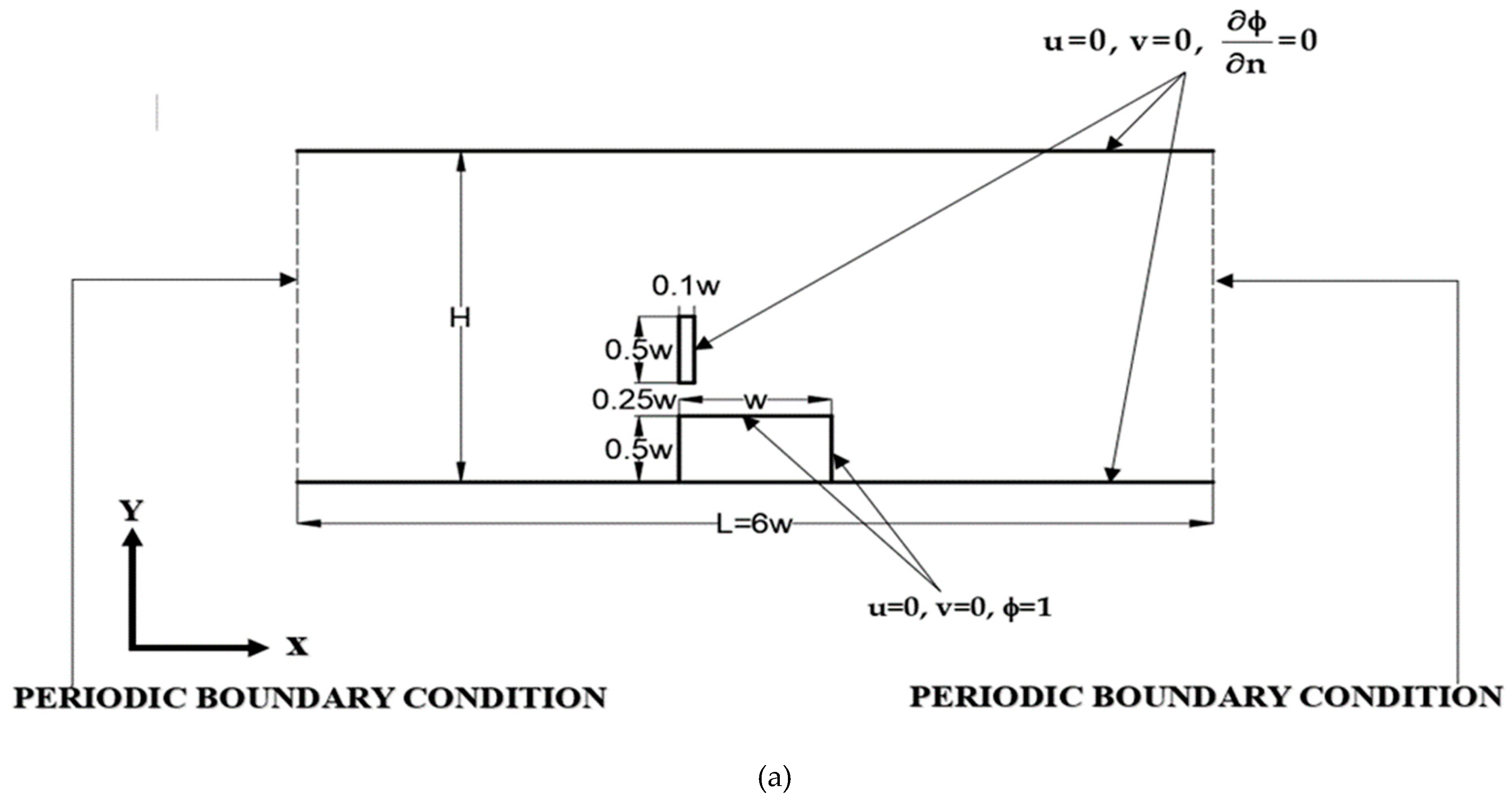
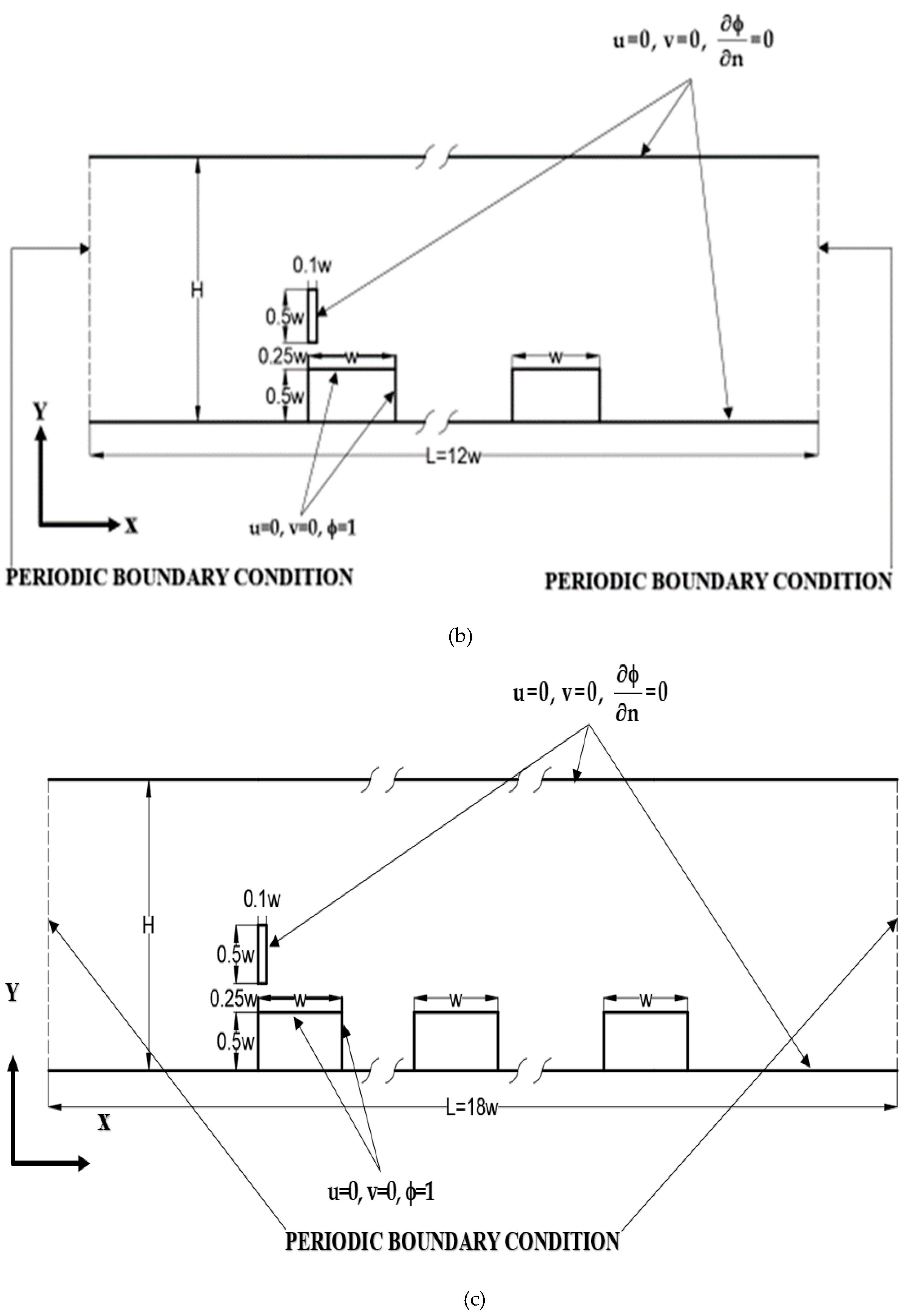
Figure 2.
Variation of time-mean Nusselt number on a heated block for Case 1 at Re= (a) 100 (b)175 (c)250.
Figure 2.
Variation of time-mean Nusselt number on a heated block for Case 1 at Re= (a) 100 (b)175 (c)250.
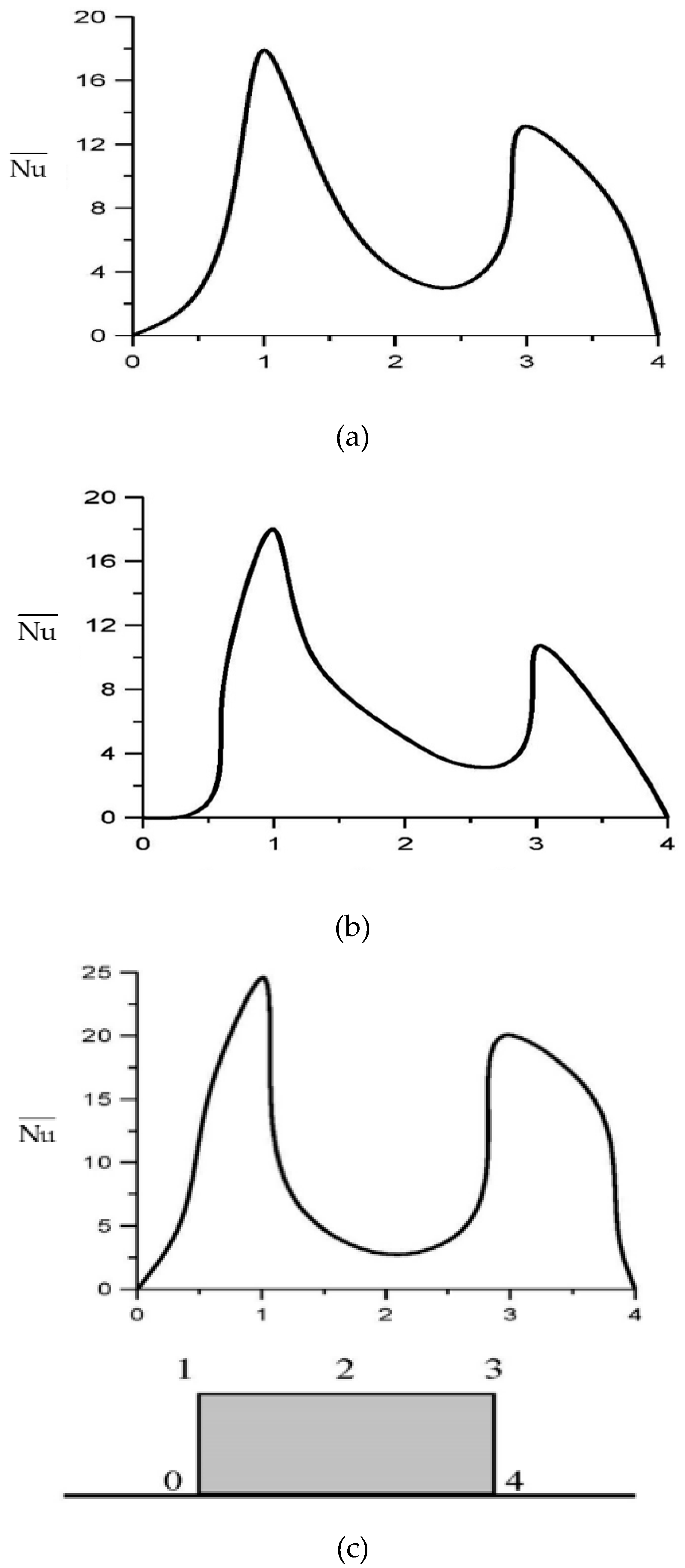
Figure 3.
Variation of time-mean Nusselt number on heated blocks for Case 2 at Re= (a)100 (b)175 (c)250.
Figure 3.
Variation of time-mean Nusselt number on heated blocks for Case 2 at Re= (a)100 (b)175 (c)250.
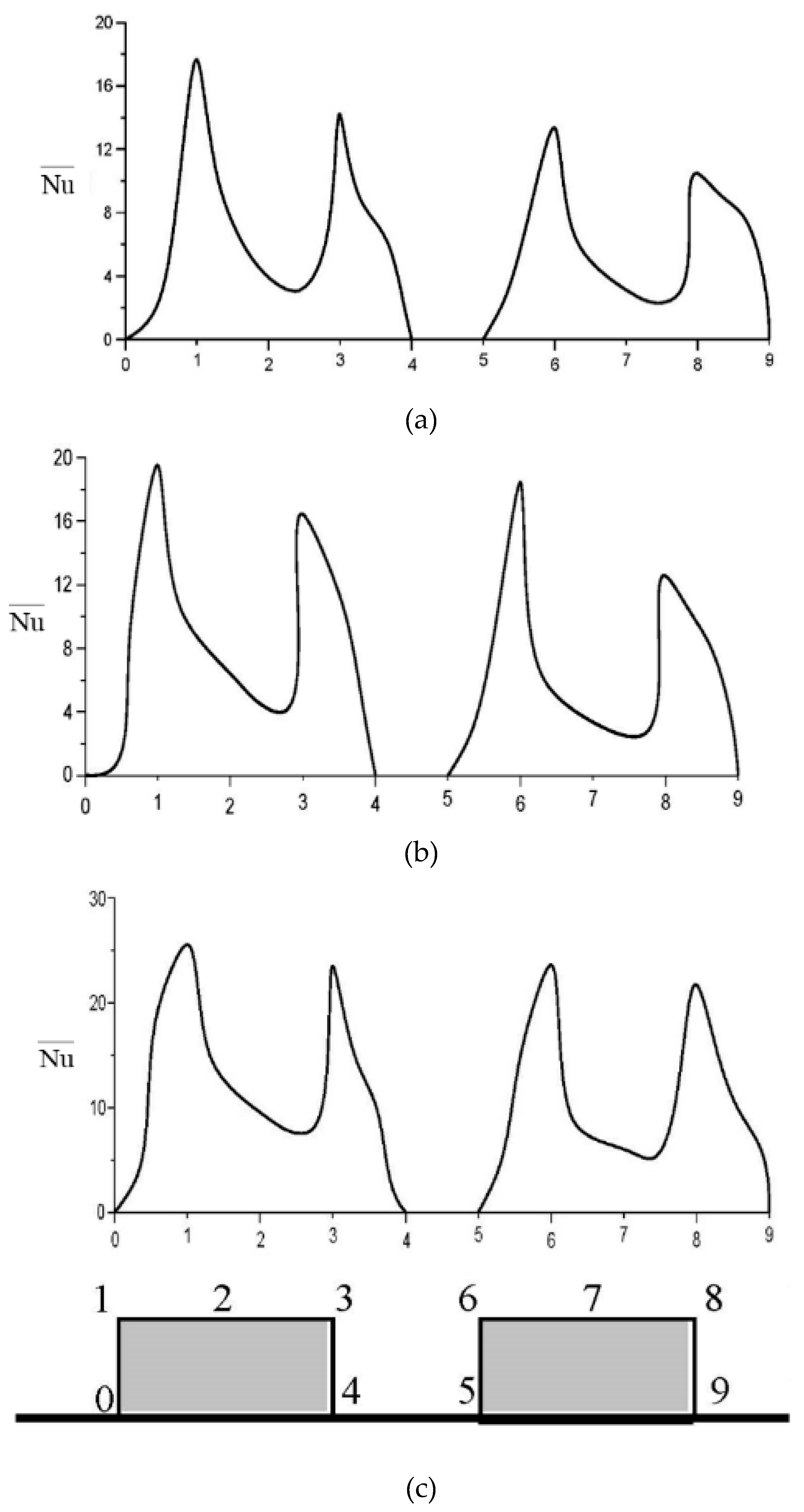
Figure 4.
Variation of time-mean Nusselt number on heated blocks for Case 3 at Re= (a)100 (b)175 (c)250.
Figure 4.
Variation of time-mean Nusselt number on heated blocks for Case 3 at Re= (a)100 (b)175 (c)250.
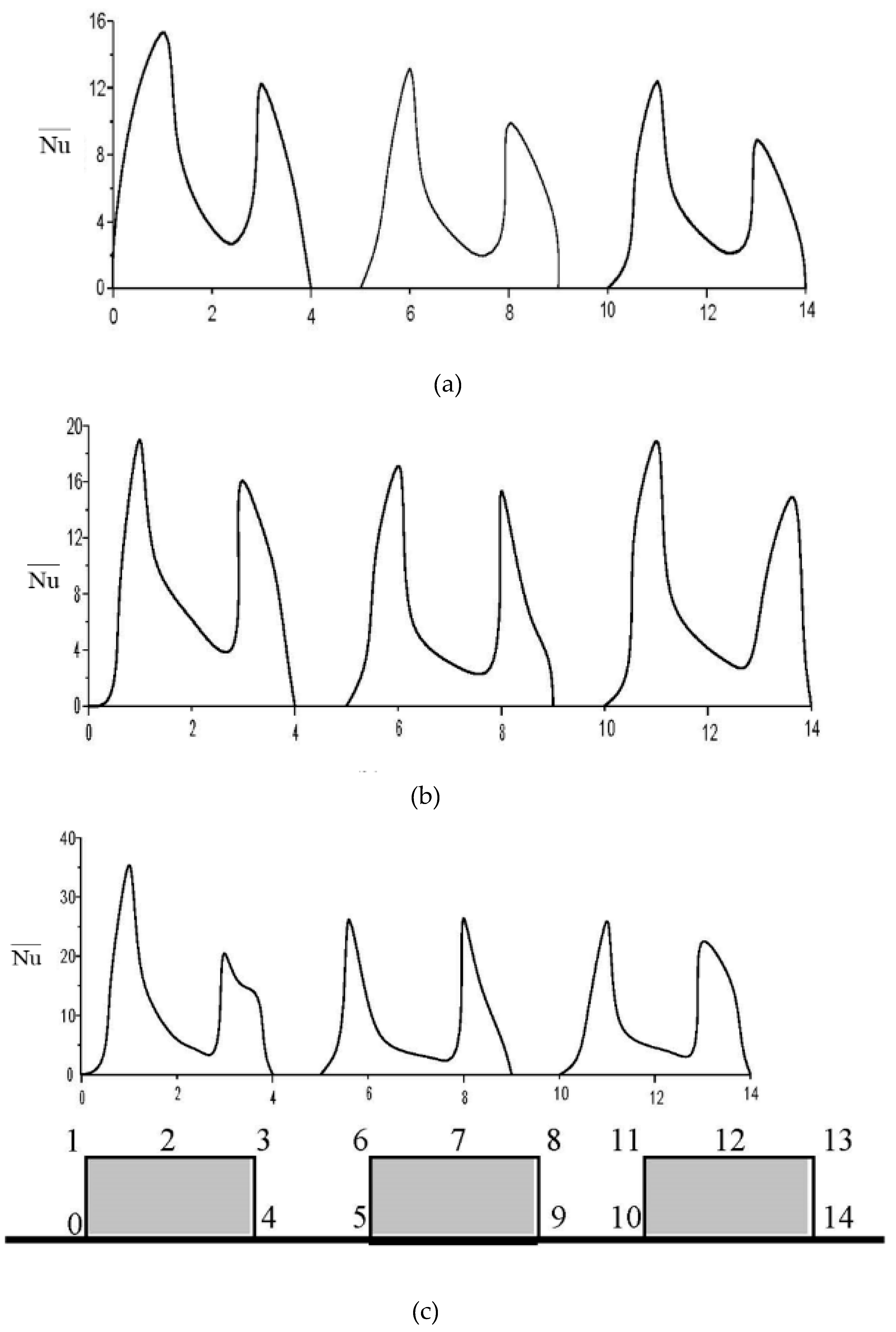
Figure 5.
Streamline patterns for periodic boundary conditions on a heated block for Case 1 at Re= (a) 100 (b)175 (c)250.
Figure 5.
Streamline patterns for periodic boundary conditions on a heated block for Case 1 at Re= (a) 100 (b)175 (c)250.
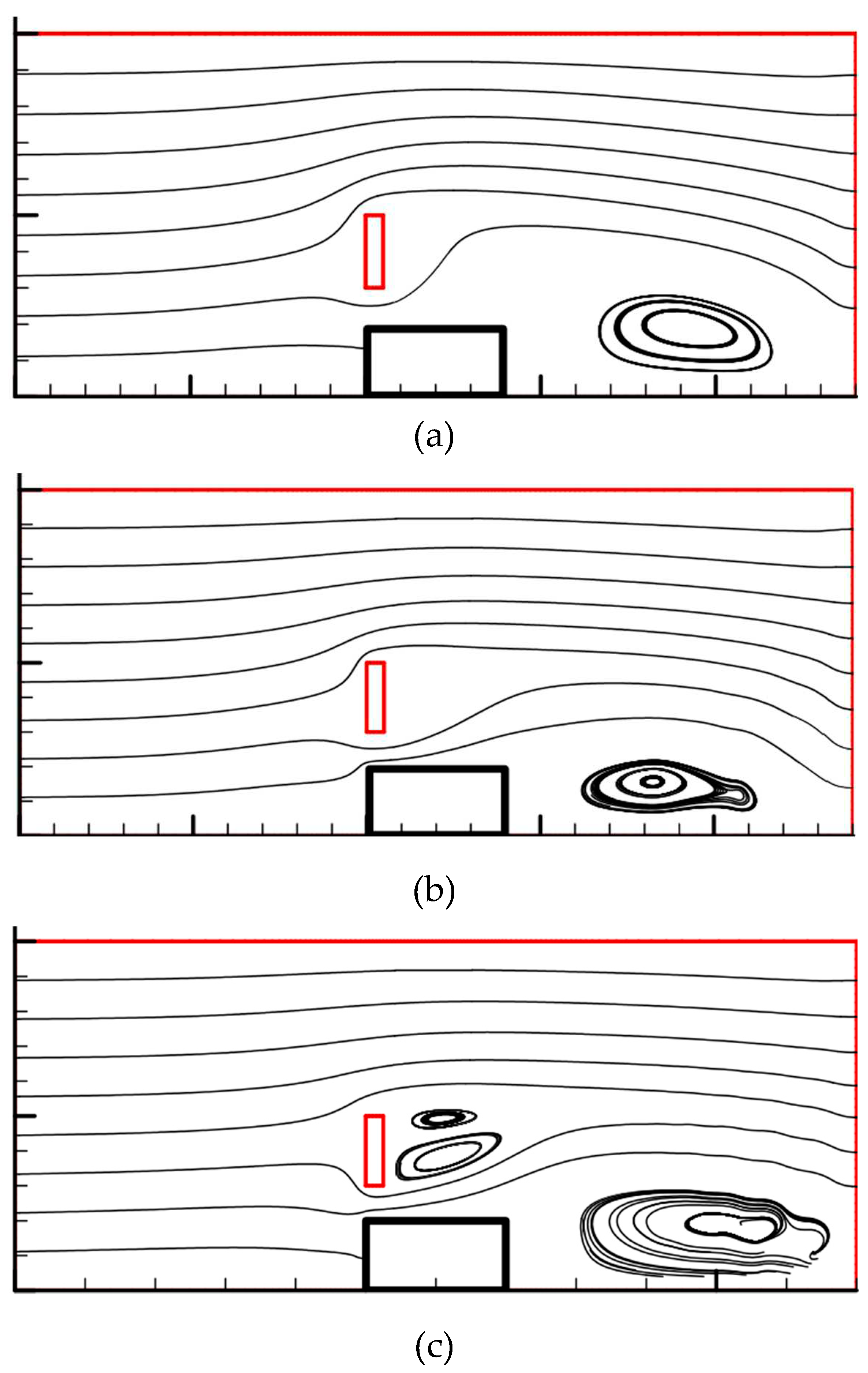
Figure 6.
Streamline patterns for periodic boundary conditions on a heated block for Case 2 at Re= (a) 100 (b)175 (c)250.
Figure 6.
Streamline patterns for periodic boundary conditions on a heated block for Case 2 at Re= (a) 100 (b)175 (c)250.
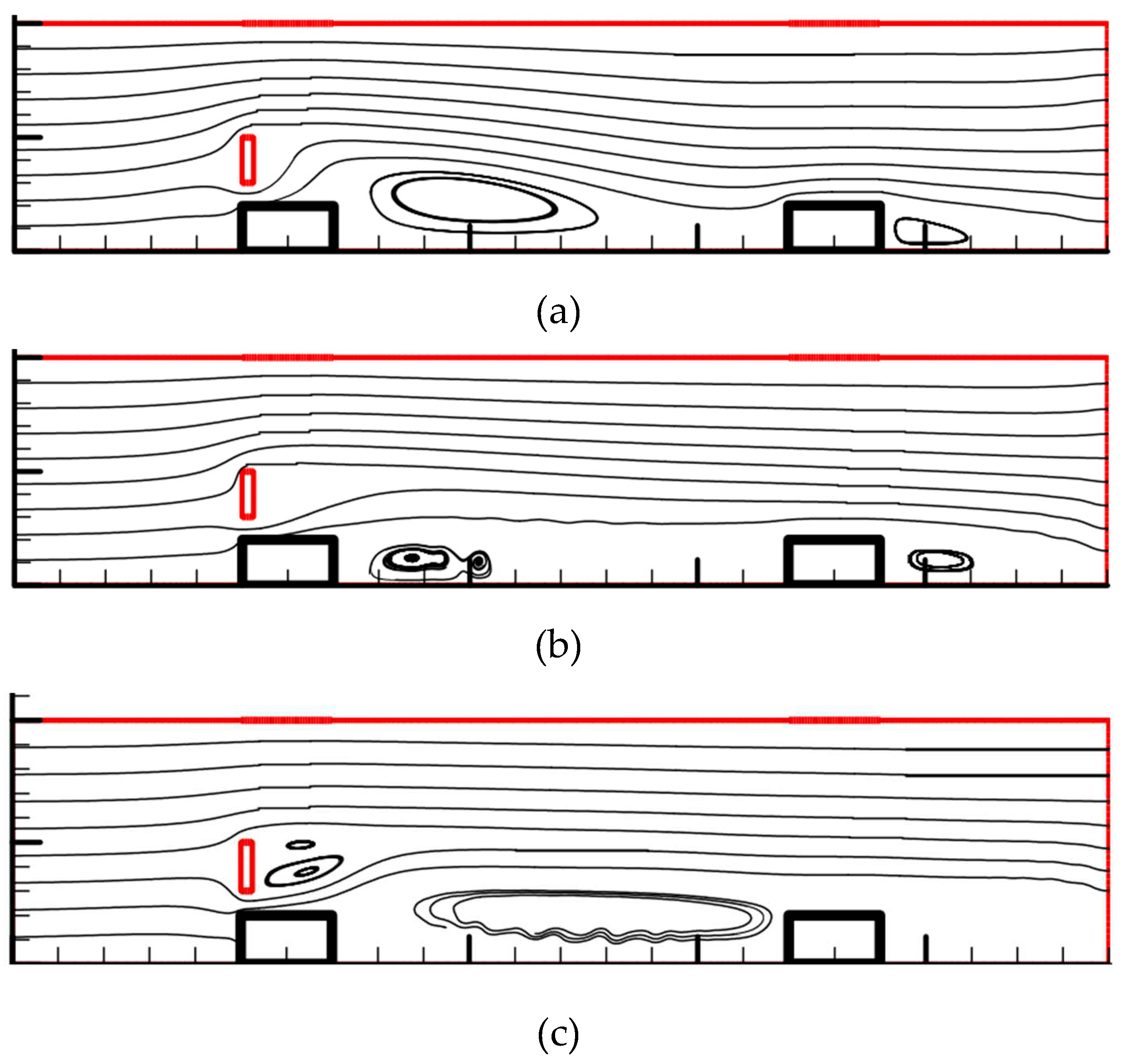
Figure 7.
Streamline patterns for periodic boundary conditions on heated blocks for Case 3 at Re= (a) 100 (b)175 (c)250.
Figure 7.
Streamline patterns for periodic boundary conditions on heated blocks for Case 3 at Re= (a) 100 (b)175 (c)250.
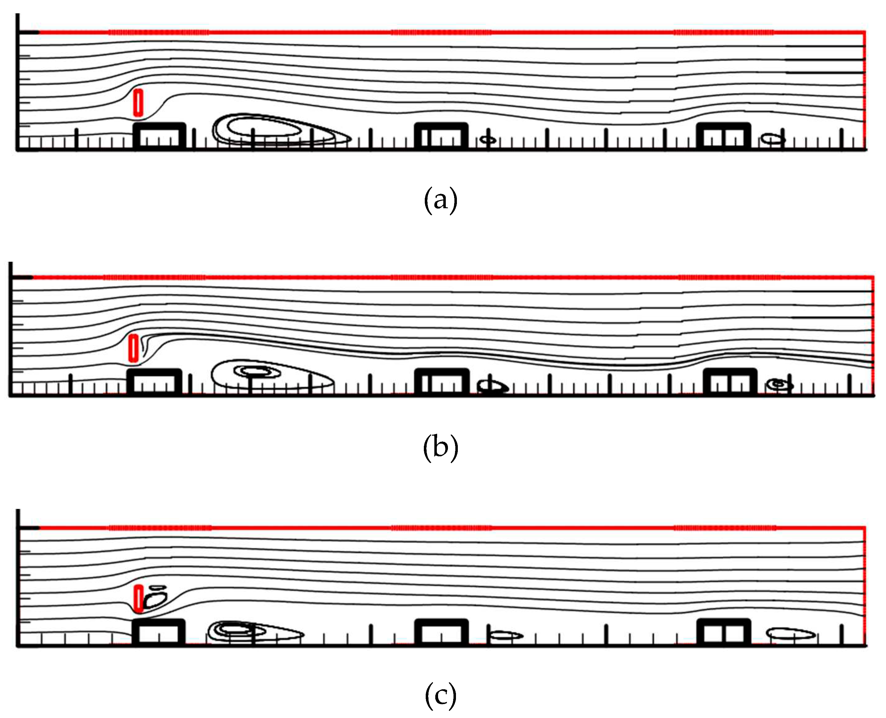
Figure 8.
Temperature contours for periodic boundary conditions on a heated block for Case 1 at Re= (a) 100 (b)175 (c)250.
Figure 8.
Temperature contours for periodic boundary conditions on a heated block for Case 1 at Re= (a) 100 (b)175 (c)250.
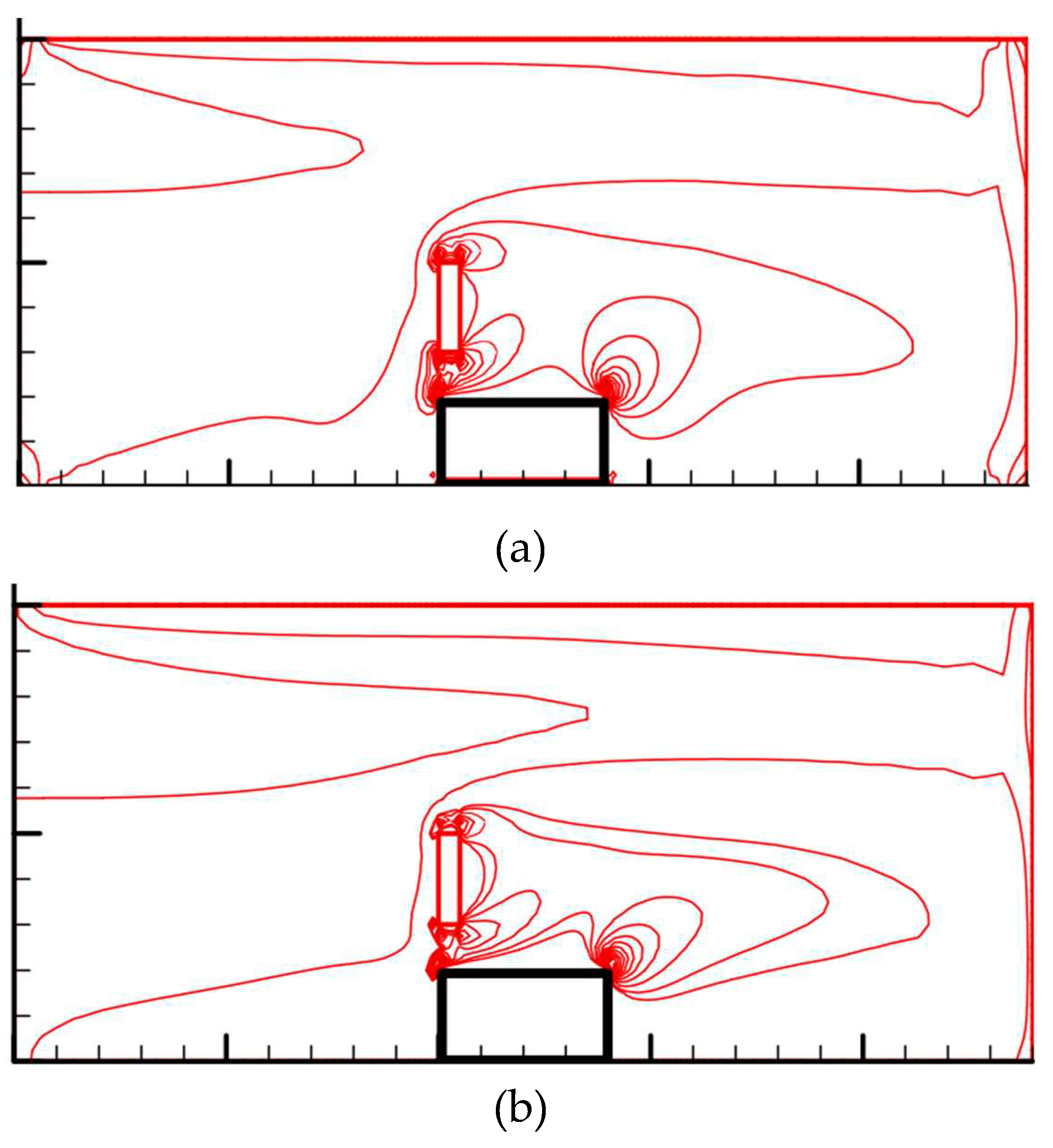
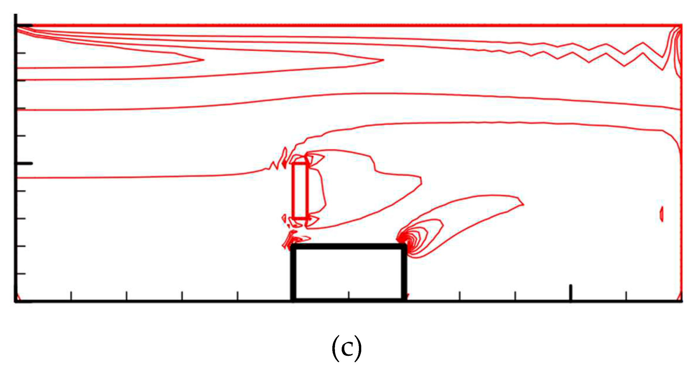
Figure 9.
Temperature contours for periodic boundary conditions on heated blocks for Case 2 at Re= (a) 100 (b)175 (c)250.
Figure 9.
Temperature contours for periodic boundary conditions on heated blocks for Case 2 at Re= (a) 100 (b)175 (c)250.
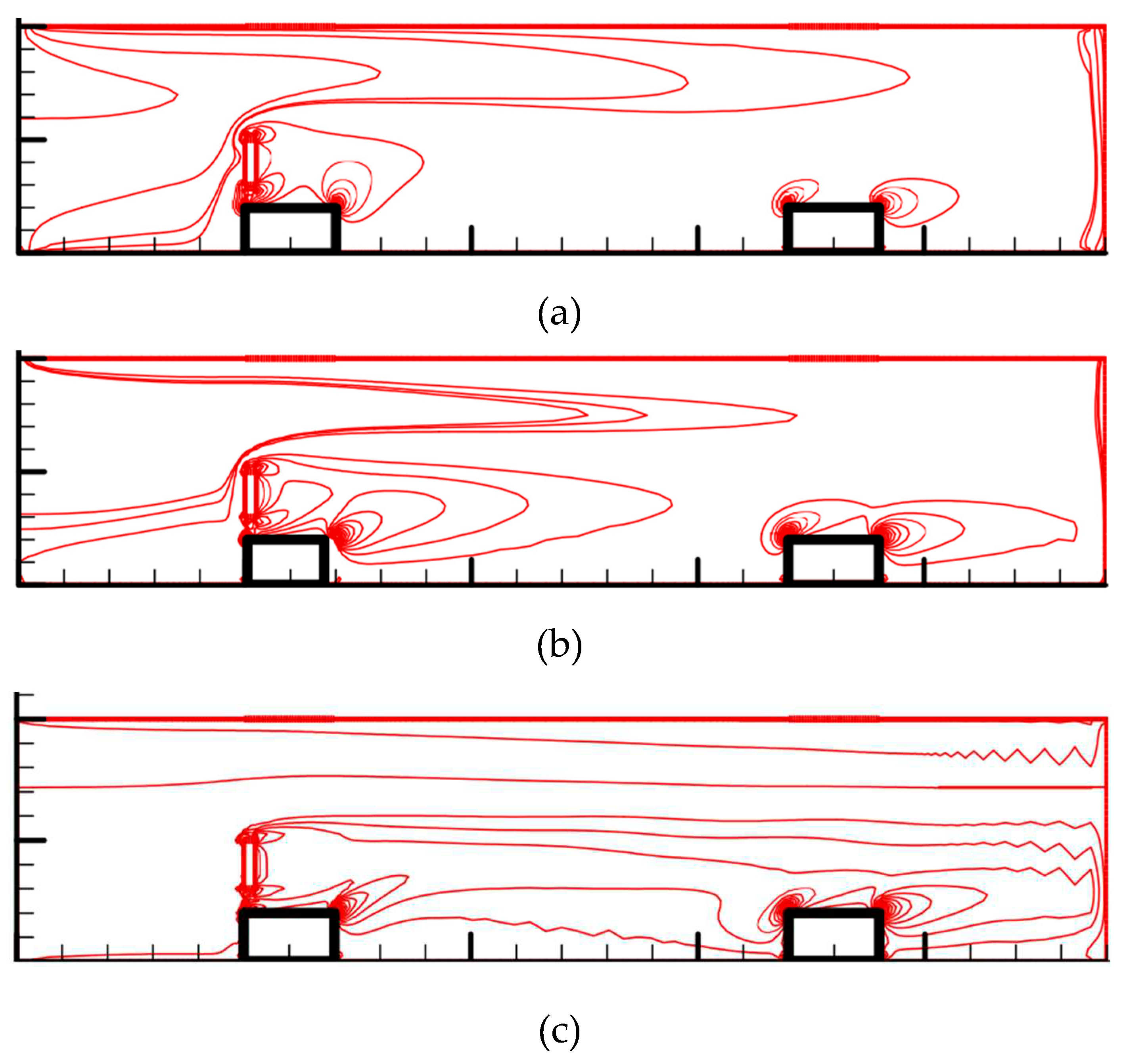
Figure 10.
Temperature contours for periodic boundary conditions on heated blocks for Case 3 at Re= (a) 100 (b)175 (c)250.
Figure 10.
Temperature contours for periodic boundary conditions on heated blocks for Case 3 at Re= (a) 100 (b)175 (c)250.
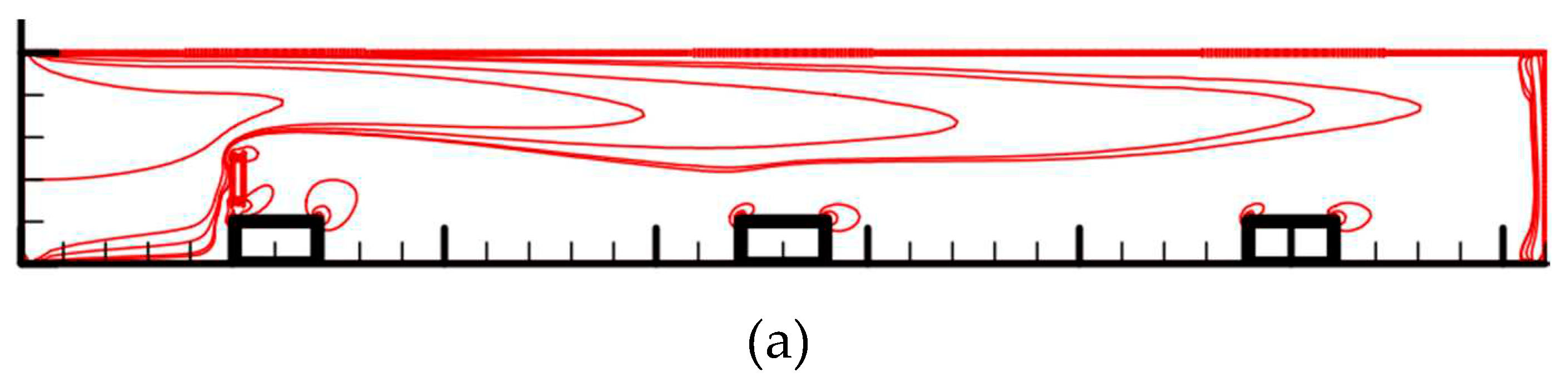
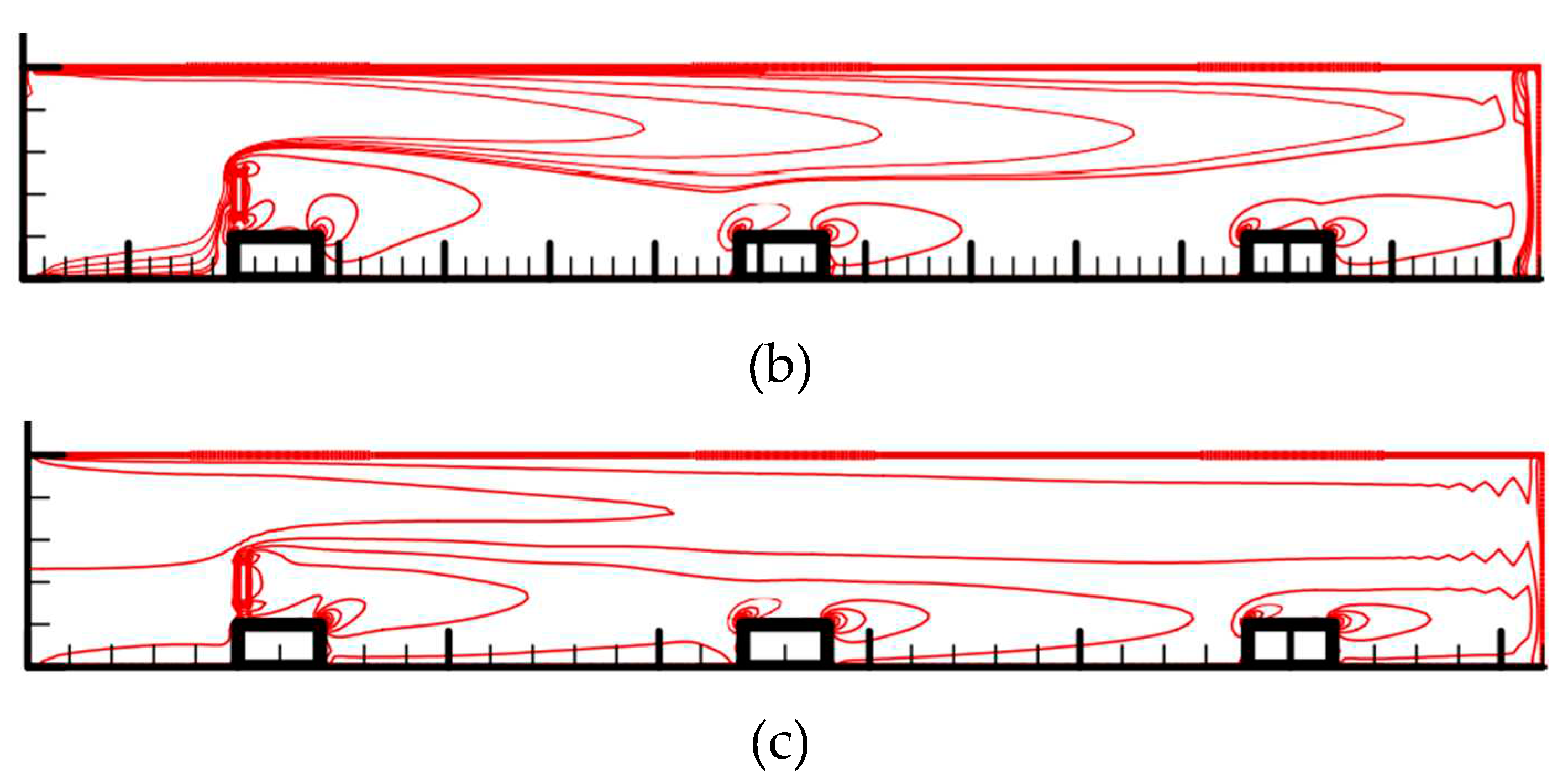
Figure 11.
(a) Variation of friction enhancement (b) Variation of Nusselt number enhancement with Reynolds number for periodic boundary conditions with various arrangements of rectangular cylinders.
Figure 11.
(a) Variation of friction enhancement (b) Variation of Nusselt number enhancement with Reynolds number for periodic boundary conditions with various arrangements of rectangular cylinders.
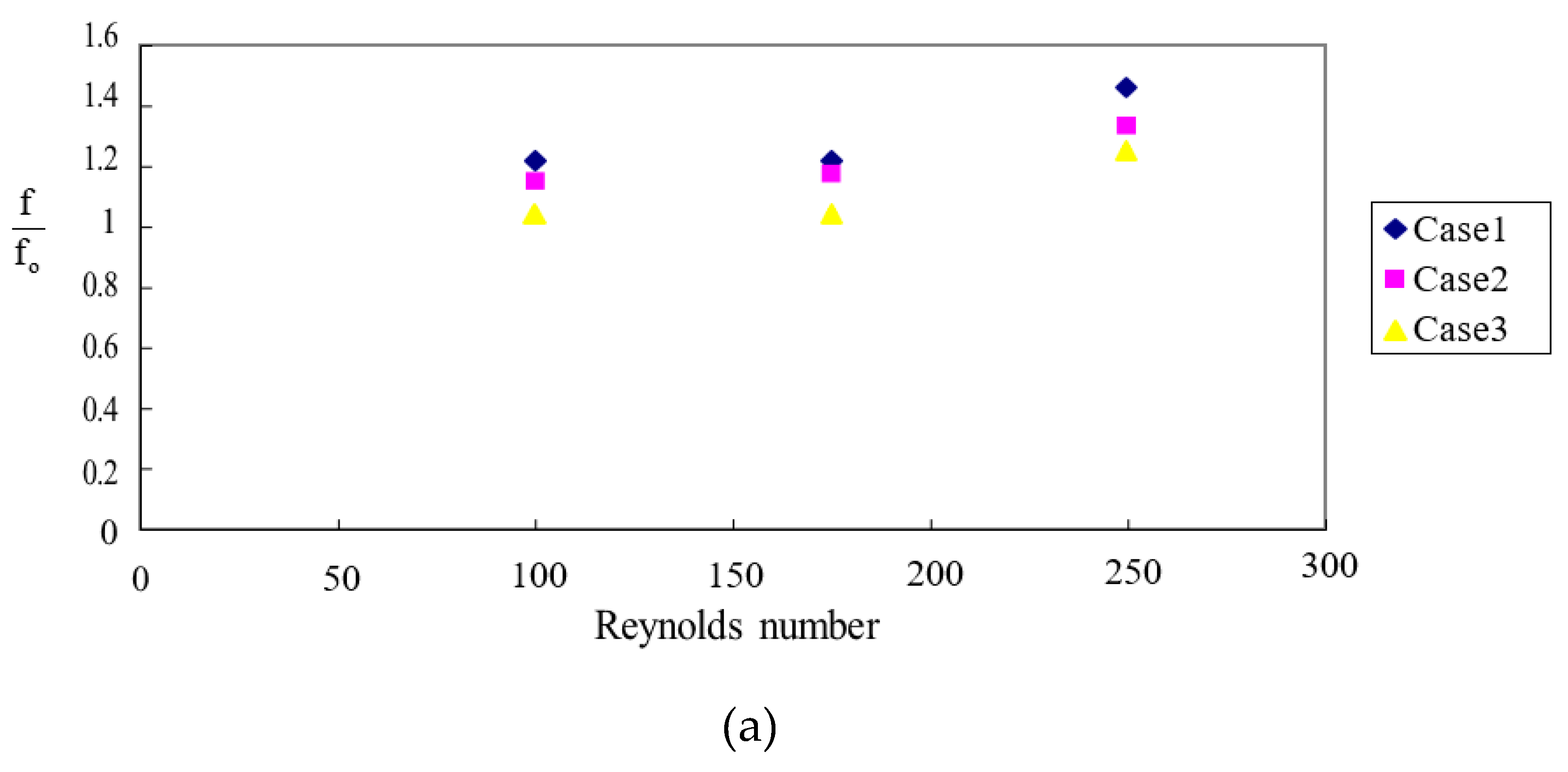
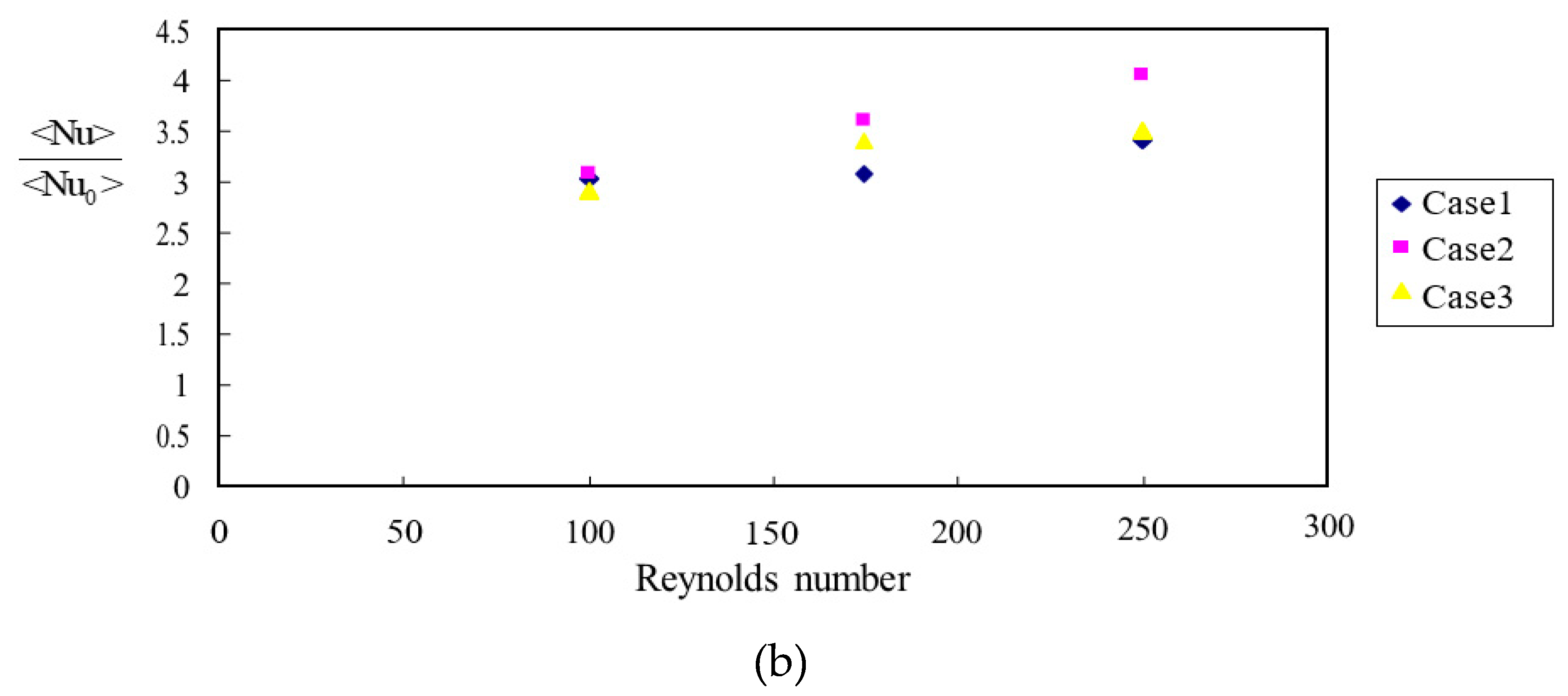
Figure 12.
Variation of thermal performance with Reynolds number for periodic boundary conditions with various arrangements of rectangular cylinders.
Figure 12.
Variation of thermal performance with Reynolds number for periodic boundary conditions with various arrangements of rectangular cylinders.
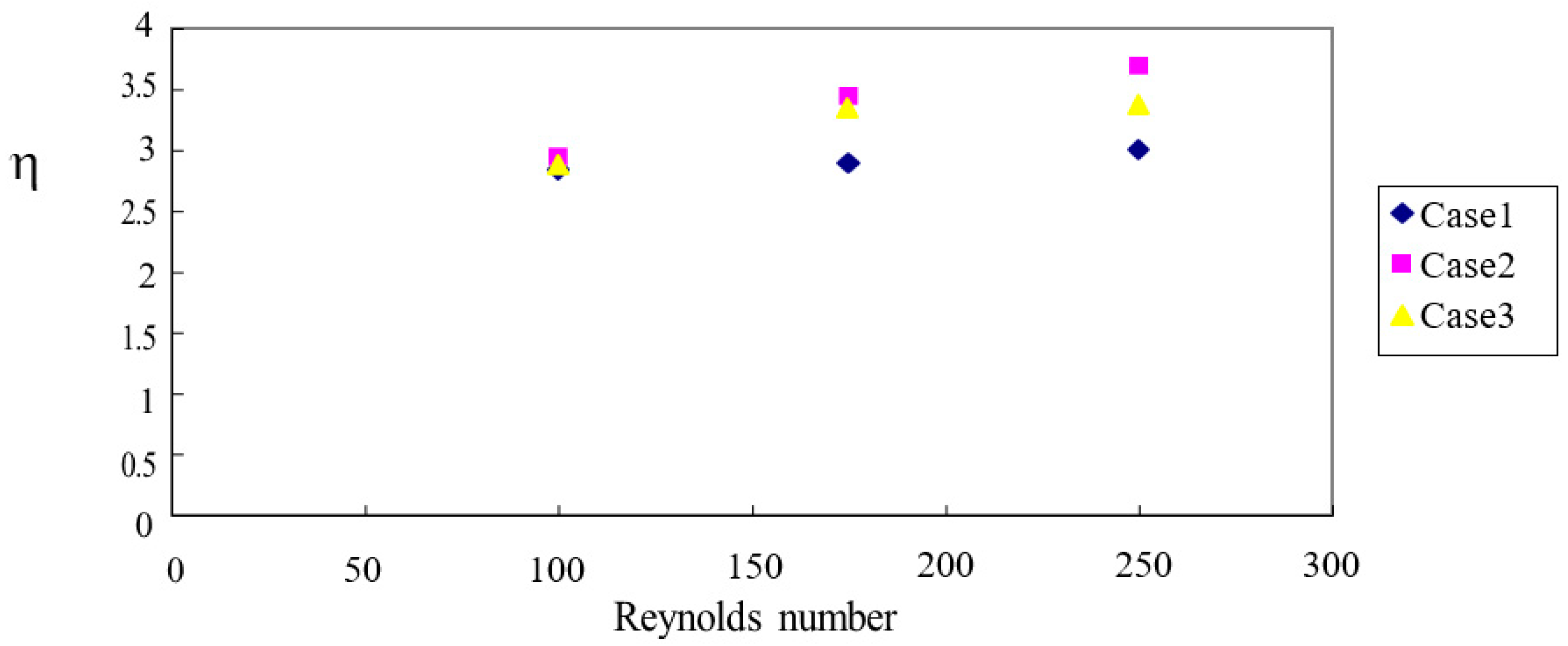

Table 1.
Mesh independent test.
| Case | Mesh |
|---|---|
| Without Rectangular cylinder |
Mesh 1 (element number: 1722;node number: 1621) Mesh 2 (element number: 3314;node number: 3164) Mesh 3 (element number: 4002;node number: 3836) |
| 1 | Mesh 1 (element number: 727;node number: 700) Mesh 2(element number: 1451;node number: 1407) Mesh 3 (element number: 2176;node number:2114) |
| 2 | Mesh 1 (element number: 1454;node number: 1400) Mesh 2 (element number: 2902;node number: 2814) Mesh 3 (element number: 4352;node number: 4228) |
| 3 | Mesh 1 (element number: 2181;node number: 2100) Mesh 2 (element number: 4353;node number: 4221) Mesh 3(element number: 6528;node number:6342) |
Table 2.
Comparison of Strouhal number St.
| Murata et al. [21] | Present paper | |
|---|---|---|
| Strouhal number | 0.30 | 0.31 |
Disclaimer/Publisher’s Note: The statements, opinions and data contained in all publications are solely those of the individual author(s) and contributor(s) and not of MDPI and/or the editor(s). MDPI and/or the editor(s) disclaim responsibility for any injury to people or property resulting from any ideas, methods, instructions or products referred to in the content. |
© 2023 by the authors. Licensee MDPI, Basel, Switzerland. This article is an open access article distributed under the terms and conditions of the Creative Commons Attribution (CC BY) license (https://creativecommons.org/licenses/by/4.0/).
Copyright: This open access article is published under a Creative Commons CC BY 4.0 license, which permit the free download, distribution, and reuse, provided that the author and preprint are cited in any reuse.


