
Submitted:
09 May 2023
Posted:
10 May 2023
Read the latest preprint version here
Abstract
To understand forest dynamics under today’s changing environmental conditions, it is important to analyze the state of forests at large scales. Forest inventories are not available for all regions, so it is important to use other additional sources of information, e.g. remote sensing observations. Increasingly, remotely sensed data based on optical instruments and airborne LIDAR are becoming widely available for forests. There is great potential in analyzing these measurements and gaining an understanding of forests state. In this work, we combine the new generation radiative transfer model mScope with the individual-based forest model FORMIND to generate reflectance spectra for forests. Combining the two models allows us to account for species diversity at different height layers in the forest. We compare the generated reflectances for forest stands in Finland, in the region of North Karelia, with Sentinel-2 measurements. We investigate which level of forest representation gives the best results. For the majority of the forest stands, we generated good reflectances with all levels forest representation compared to the measured reflectance. Good correlations were also found for the vegetation indices (especially NDVI with R²=0.62). This work provides a forward modelling tool for relating forest reflectance to forest characteristics. With this tool it is possible to generate a large set of forest stands with corresponding reflectances. This opens the possibility to understand how reflectance is related to succession and different forest conditions.
Keywords:
forest model
; radiative transfer
; vegetation indices
; individual based
; forest reflectance
1. Introduction
Forest play a major role in the terrestrial component of the global carbon cycle. They account for about 55% of global forest aboveground carbon stock [1] and represent approximately 40% of the global terrestrial carbon sink [2,3]. Forests shape the surface of the Earth by comprising 31% of the land area [4] and they influence the energy balance by reflecting and absorbing sunlight. They are important for sustaining biodiversity and provide habitat for 70% of all faunal species [5,6,7]. Forests exhibit a diversity of spatial structures that can be dynamic due to natural succession, management or disturbances [8].
To monitor the state of forests, the conventional standard practice for foresters and ecologists alike has long been measurement of forest inventories. Collecting inventories is time consuming. However, in tropical forests, national forest inventories are often missing. Another approach to monitor forests is based on remote sensing observations which provide relevant data at large scales. The amount of data is significantly raising with more and more earth observing satellite missions that were launched in the last ten years [9]. The spatial and temporal remote sensing observations offer the opportunity to get a better understanding of forests with respect to their structure and dynamics. Satellite measurements vary in their resolution and coverage. Thus, for global observations, there is a trade-off between the spatial and temporal resolution of satellite (e.g., Landsat, Sentinel) and airborne products. The combined methods of remote sensing and field observations offers the opportunity to get a better understanding of forests with respect to their structure and dynamics. However, the ecological interpretation of remote sensing observations of forests is challenging, and in many cases still in development.
One way to obtain information from remote sensing measurements concerning target vegetation variables (e.g. LAI, species composition, productivity), is to use models that link the measured remote sensing measurements to the vegetation. Vegetation models have been successfully applied to study change in forests for nearly four decades, many of which differ in their applications. One example, dynamic global vegetation models (e.g. ED by [10] and CLM4 by [11]) were initially developed to represent the interaction between vegetation and the global carbon cycle as stand-alone simulation models, but also to represent vegetation dynamics in the context of Earth System Models, or alongside atmospheric (General Circulation Models), oceanic, and the cryospheric modeling frameworks [12]. These models focus on large scale applications and they rely on simplifications to reduce complexity and computational demand (e.g. individual species simplicated to plant functional types). They do not offer information at the individual tree level. For the analysis of forests in forestry and ecology, there is a long tradition [13] of using individual forest models (e.g. FORMIND by [14] and LPJ-GUESS by [15]). They are able to represent the ecosystem dynamics of the forest by simulating each individual tree in a forest. At the same time, with increasing computing capacity, there is an opportunity to use these models to simulate large areas. Due to the simulation of single trees, they are also able to consider the heterogeneity of forest structure and dynamics.
An important component in vegetation models is solar irradiance and the competition for light between plants. One simple way to calculate the light climate is based on Lambert-Beer’s law, which is often used by forest models. It describes the decreasing intensity of radiation as it passes through a medium (e.g. tree crowns), depending on the composition of the medium and the height of the layer. Radiative transfer models (RTMs) calculate the light climate in the forests in a more detailed way. They simulate the reflectance, interception, absorption, and transmission of light through a canopy. Due to this, they are not only able to calculate the availability of light for plants, they can also calculate the reflectance of the canopy, that can be measured by satellites. Canopy radiative transfer is one of the primary and long relied upon mechanisms by which models relate vegetation properties to surface reflectance as captured by remote sensing [16] radiative transfer in combination with vegetation can be modelled in different levels of complexity. The vegetation can range from a simple homogeneous forest to a 3D simulation of the vegetation structure. The complexity of the solution of radiative transfer problems also varies [17,18] from numerical Monte Carlo ray tracing approaches (e.g. [19,20]) to analytical solutions using e.g. four stream technology (e.g. [21]).
Some of the global vegetation models are coupled with a nontrivial radiative transfer model to calculate reflectance for wavelength from 300 to 2500 nm. The two-stream approximation is used to calculate radiative transfer in CLM4.5 [22], ED2 [23] and CLM(SPA) [24]. Mostly these model’s use only a few plant functional types and a low number of canopy layers.
With the new generation of RTMs (like DART by [25] and mScope by [26]) it is possible to consider heterogeneous vegetation. The more complex the structure of the vegetation is, the more computationally intensive the simulation of light reflectance and the interaction with the vegetation. The same applies to the simulation of vegetation on a global level. As mentioned, global vegetation models must make strong simplifications in order to be able to simulate large areas in appropriate timespans. Individual-based models describe forest structure in a more detailed way, but they are difficult to apply on a global scale because of the computational requirements. Nevertheless, they endorse the fundamental premise that the structure of forests represents an important factor for ecosystem dynamics that is lost in more aggregated modelling approaches [13].
Individual based forest models in combination with the new generation of RTMs are therefore a promising approach to consider the complexity of forest structure and species. Their combination will aid in the development of a mechanistic understanding of the linkage between forest reflectance and forest properties like structure and species diversity. The challenge is to develop an approach which is sensitive to forest structure and species diversity within the current, but ever-increasing computational constraints both in simulating vegetation and radiative transfer, in order to allow the analysis of huge forest simulations. Such a tool can be also used to get a more general understanding of the relationships between reflectance and vegetation properties.
Here, we present an approach by coupling the RTM mScope with the individual-based forest model FORMIND. We enlarge the application field of mScope and investigate the calculated reflectance spectra of boreal forests using forests in Finland as an example. Comparing the simulation output with Sentinel-2 data allows us to answer the following questions: How does the concept of forest representation in the model influence the reflectance spectrum? Can the approach reproduce the variety of reflectance spectra in Finland? And how well can we calculate the vegetation indices of the forests with this approach?
2. Materials and Methods
By coupling the individual-based forest model FORMIND and the radiative transfer model mScope, we combined a new-generation RTMS with an individual based forest model. For this purpose, we have implemented mScope (adapted version) in c++ as an additional module in the forest model FORMIND. By using inventories for forest stands in Finland and the forest model, we are able to reconstruct the forests in Finland. In combination with the RTM it is possible to calculate the reflectance spectra from forests (visual and near infrared). We compared the simulated reflectance with measured reflectance spectra from remote sensing observations (Sentinel-2). To analyze possible applications, different levels of the forest complexity were analyzed and their influence on the reflection spectra was investigated. In addition, several vegetation indices were calculated and analyzed.
2.1. Application of the individual-based forest model FORMIND to a Finland forest inventory
For the simulation of the forest stands we used the individual- and process-based forest model FORMIND, which belongs to the model family of individual-based forest gap models. This forest model allows the simulation of forests with different tree species and also considers the size structure of the tree community. FORMIND has been extensively tested and applied to tropical forests [27,28,29,30,31,32,33,34,35], temperate forests [36,37,38], grasslands [39] and boreal forests [40]. It is an individual-based forest model which means that the growth of every single tree is simulated. The model includes four main process groups: growth of single trees (increment of tree biomass, stem diameter and height), mortality, recruitment, and competition (e.g. for light and space). FORMIND is also used for large scale simulations [35,41] e.g. in the Amazon.
For this study we investigated forest stands in Finland, in the region of North Karelia, for which inventory data is collected for the FunDivEUROPE project (http://www.fundiveurope.eu) [42]. Twenty-eight forest stands were measured in the years 2012 and 2017. For the initialization of the forest model (here FORMIND), species information, tree positions (X- and Y-coordinates) and stem diameters of the two forest inventories are used (to reconstruct the steam diameter in 2015, we calculated the average stem diameter of both forest inventories). Based on stem diameter and tree species, all other forest attributes, such as tree height, crown diameter, LAI are calculated by the forest model using species specific allometric equations which are included in the parameterizations of the forest model [36]. The simulated forest stands are 30 m × 30 m and shown in Figure 1. They are distributed over an area of 150 km × 150 km.
We then compared the calculated reflectance spectra with remote sensing observation susing atmosphere-corrected Sentinel-2 measurements [43] from 2015. For the simulation of the reflectance spectra, information on observation geometries (sun and observer, in terms of zenith and azimuth) for each forest stand is available. The measured reflectances (Sentinel-2) were used for comparison with the simulated reflectances.
2.2. Coupling the radiative transfer model mScope [26] with FORMIND
We use the radiative transfer model mScope [26] to simulate the reflectance spectra of forest stands. MScope is a modified version of the Scope model [44]. The Scope model is a vertical one dimensional, integrated radiative transfer and energy balance model, which simulates short wave reflectance spectra (400 – 2500 nm) of homogeneous vegetation. Compared to Scope, mScope has multiple layers to simulate different structure of vegetation which enable the representation and simulation of heterogeneous vegetation. As leaf model we use PROSPECT-D [45].
For the parameterization of the leaf model following attributes are used:
- leaf structure (number of internal leaf layers [layer])
- the amount of pigments in the leaf (chlorophyll a and b [], carotenoids [], anthocyanins [], senescent pigments [fraction])
- dry matter [] and leaf water content []
- traits describing vegetation structure as the mean and bimodality of the leaf inclination distribution function, leaf area index ], canopy height [m]
The parameters for the different species were taken from the “CABO 2018-2019 Leaf-Level Spectra Data set” by [46].
Using the individual-based approach in forest modeling, it is possible to simulate and describe forest structure at fine scales, which allows for the heterogeneity of a forest to be considered. Individual-based forest models (here FORMIND) make it possible to gain, tree- and forest-specific properties for each forest patch (e.g. 30 m × 30 m) in different height layers (each height layer has a layer height, here 0.5 m). One important property to calculate radiative transfer is the LAI. The model enables the calculation of LAI distributions for each tree over height. In order to determine the species composition, we used the LAI fraction of a species as a measure of its abundance. MScope uses a fixed number of height layers (in the basic version: 60 layers). In our modified version we used a fixed layer height of 0.5 m and a variable number of layers (e.g. 82 layers for a maximum tree height of 41 m).
To calculate leaf reflectance and transmittance (using the leaf model Prospect D), the radiative transfer model utilized information from the forest model for each layer, which included a leaf parameterization containing leaf properties for each layer. Additionally, the distribution of the orientation of leaves was considered – it was assumed to be spherical for all species. MScope also includes observation geometry (sun and satellite, azimuth and zenith). Vegetation information from the reconstructed simulated forest, which is delivered by the forest model was able to be processed in different ways and then be transferred to the radiative transfer model. In this paper, we analyzed three cases, for which each consequence to a different representation of the vegetation. The processing differs according to the LAI and according to the species composition (Figure 2).
-
Simple forest representationThe simplified forest representation, uses only reduced information of the forest. It assumes the same mixture of species and the same LAI for each height layer of the forest stand. The leaf parameterization is calculated by averaging the leaf attributes of the occurring species (weighted by LAI, as a measure of abundance). The LAI of the forest stand is equally distributed among all layers.
-
Detailed forest representationThe detailed representation of the forest, assigns to each height layer different mixtures of species and different LAIs. The leaf parameterization for each layer is calculated by averaging the leaf attributes of the occurring species weighted by LAI in the height layer, as a measure of abundance. For each layer of the forest, the calculated LAI of the reconstructed forest stand will be used.
-
Spectra-averaged representationIn this case, the forest is divided into different “sub-forests”. In each sub-forest stand, we maintain the total number of trees and the structure of the main forest stand. However, we assume that all trees in a sub-forest stand are of only one species. Thus, there are as many sub-forests as there are tree species. For each layer, the calculated LAI of the reconstructed forest stand is used. For each of these single-species sub-forests, the reflectance spectra are calculated using the species-specific leaf parameters. Final reflectance spectrum is determined by averaging the species-specific spectra weighted by LAI fraction, as a measure of abundance.
The processed Sentinel-2 observations [43] include reflectance values for 10 wavebands. For better comparability with the simulated reflectance profiles, we averaged the simulated reflectance values in the band range (shown in dots in Figure 3 and 3).
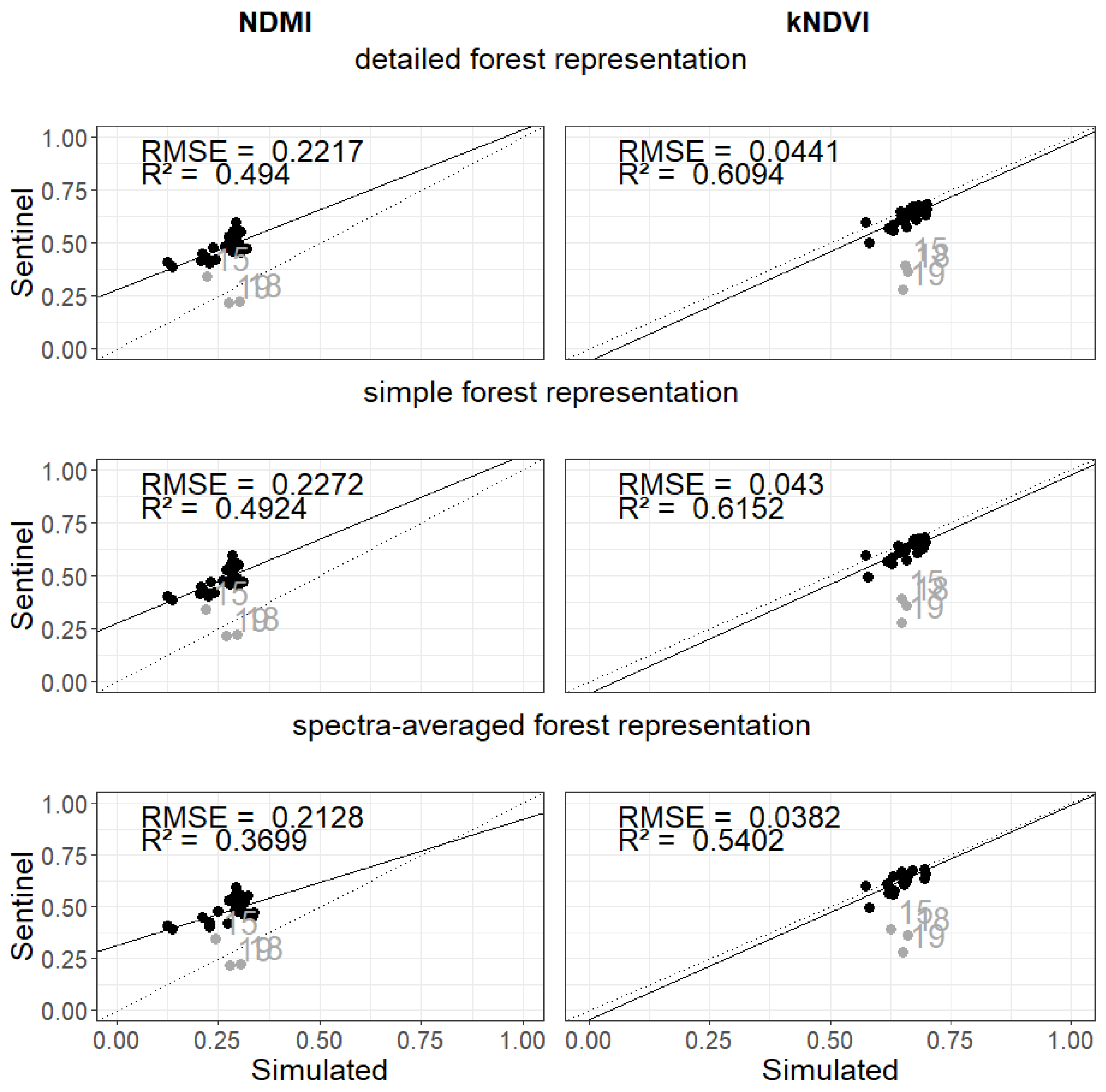
Vegetation indices derived from canopy reflectance are widely used in remote sensing, as they represent proxies for vegetation attributes (e.g. LAI, productivity). We calculated several vegetation indices (NDVI, EVI, MSI, in appendix: NDMI, kNDVI). NDVI is chlorophyll sensitive. EVI [47] is responsive to canopy structural variations, including LAI, canopy type and plant physiognomy [48]. We also analyzed kNDVI [49] as a modification of the NDVI. The NDMI is partly correlated with the water content of the canopy [50]. [51] introduced the moisture stress index (MSI, [52]), which utilises reflectance wavebands in the SWIR (1550 - 1750 nm) and NIRS (760 - 900 nm).
In the mScope model, some code adjustments were made to account for the structure of the forest models and forests from the inventory. In forests models it is possible that there are layers without leaves (vertical gaps). The adjustments were necessary to ensure that these layers had no influence on the reflectance spectrum. MScope calculates the probability of viewing a leaf in solar () and observer direction () by assuming a homogeneously distributed LAI in the forest.
with as negative cumulative layer thickness, k as extinction coefficient in direction of sun, as Leaf Area Index of forest stand and K as extinction coefficient in direction of sun.
This leads to the situation that the probability is also influenced by layers with a LAI of 0. We have changed the calculation equivalently allowing different LAI values for the height layers.
with as Leaf Area Index in height layer i of forest stand, k as extinction coefficient in direction of sun and with K as extinction coefficient in direction of sun.
The mScope code also includes a correction of and , which we also considered.
3. Results
First, we analyzed the reflectance of even-aged forests, where the RTM used 10 m height layers (Figure 3). The even-aged forest stands no. 17, which was dominated by one species and stand no. 5 which contained three species were used as examples for this analysis. Reflectance was then calculated for simplified and detailed forest representations.
Figure 3.
Reflectance spectra for detailed and simplified forest representation by using layers of 10 m height. Visualization of the calculated reflectance profiles for two forest stands (no. 5 and 17) in Finland. Forest stand no. 17 (left - mainly one species) and forest stand no. 5 (right - three species). Both forest stands are even-aged (small standard deviation of tree heights: 4.6 m and 4.5 m). Each point represents the reflectance value averaged over the specific bands (corresponding to the bands of Sentinel-2). Sentinel measurements are shown in black and simulated reflectance is shown in orange/blue from coupling a forest model (FORMIND) with mScope. We used 10 m height layers. The reflection of all other forest stands is shown in the Appendix (Figure A2).
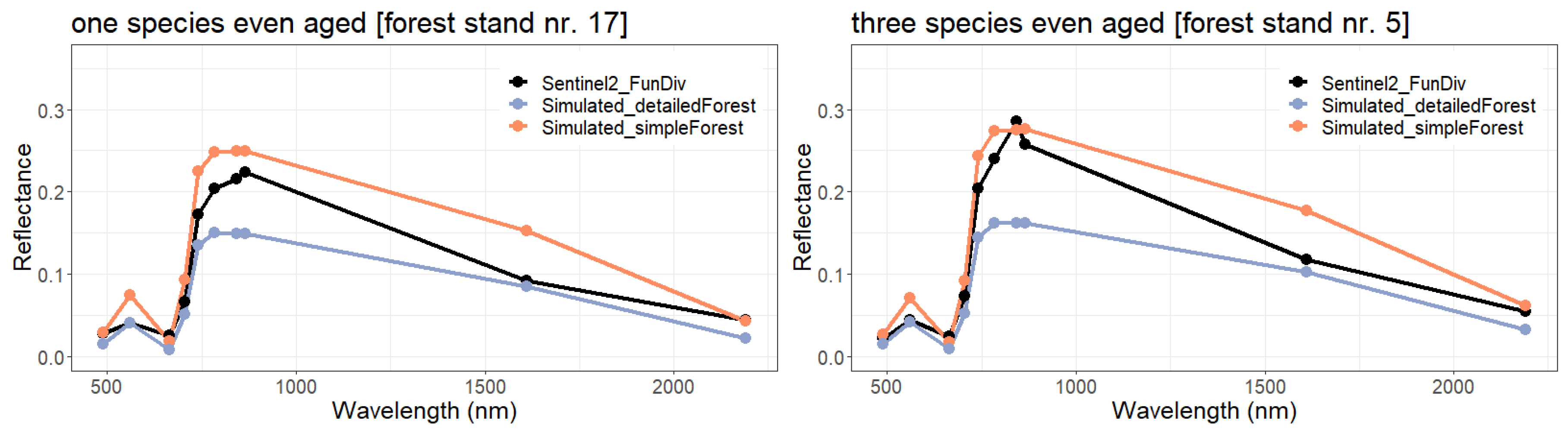
There were differences (up to 140%) in reflectance between the detailed (blue) and the simplified (orange) forest representation. The simplified representation consistently produced higher reflectance. Both the modelling and satellite measurements show different reflectance spectra for the two forests. We found a higher similarity of reflectance for the detailed representation.
In the next part of the investigation, we increased the represented complexity of the forest. This was done by assuming a layer height of 0.5 m (Figure 4). Here, the forest model (here FORMIND) provided mScope with a higher resolution distribution of LAI and species-specific information over height. As in Figure 3, results are again shown for both the simplified and the detailed representation of the forests for both example sites. Additionally, the spectra-averaged forest representation has been analyzed.
All three versions produced comparable reflectance spectra (especially for forest stand no. 17). The lowest reflectances were produced with the spectra-averaged forest representation (in particular for forest stand no. 5). For forest stand 17 the spectra-averaged forest representation produces the same reflectance values as the detailed forest representation version. As the forest stand contains only one species, there is no averaging in the leaf parameters and spectra, and we got the same results for these versions. Results for all bands were in agreement with the sentinel measurements.
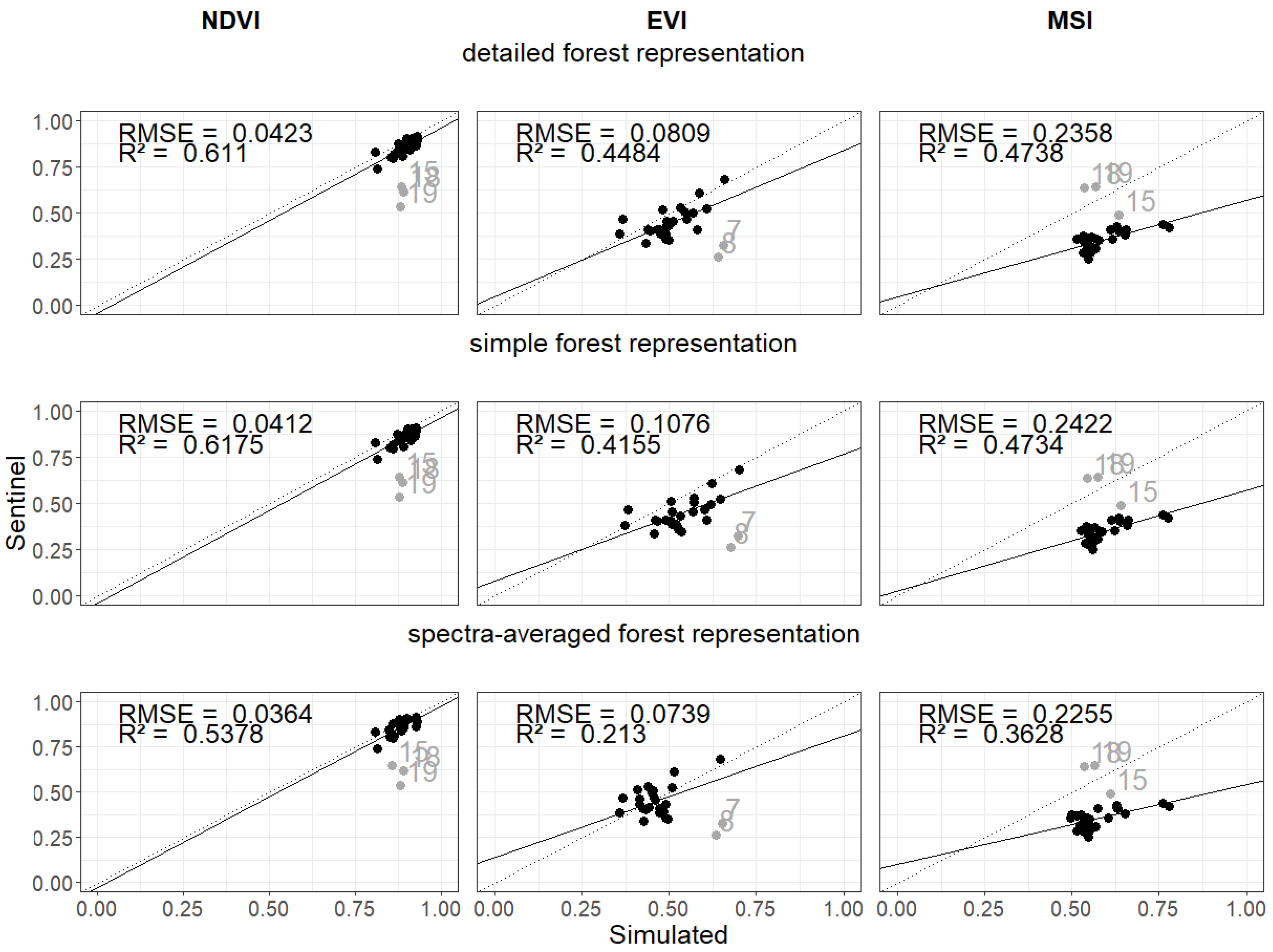
The simulated reflectance spectra also enabled the calculation of vegetation indices (see Section 2.2). We analyzed NDVI, EVI and MSI (kNDVI and NDMI in appendix Figure A13) for each forest stand and for each forest representation (Figure 5). Each were then compared with indices calculated using the satellite observations.
We obtained different results for all 3 forest representations when analyzing NDVI, EVI, and MSI. Lower and higher RMSE values are obtained for MSI. Measured Sentinel-2 values were close to each other. NDVI values from simulated reflectance spectra were within small ranges. We found an of 0.61 (detailed forest representation) when comparing simulated and measured NDVI values. For the EVI, there is a larger range of values. EVI led to a lower (about 0.45) and higher RMSE (0.08) for compared to NDVI. Detailed and simple forest representation show similar results for all three indices
4. Discussion
In this work, we developed a new approach to study forest reflectance for light in the visible and near infrared spectrum. For this, we coupled the individual-based forest model FORMIND with an adapted version of the radiative transfer model mScope. We then used the coupled models to reconstruct 28 forest stands in Finland and calculate reflectance spectra for each. We analyzed three different concepts of forest representation: simple, detailed and spectra-averaged.
When we compare the simulated reflectance spectra with the sentinel measurements, the best results where achieved for the detailed forest representation. However, measured and simulated reflectance can show large differences in a few cases. Analysis of these cases (outliers) suggests that factors other than LAI distribution and species composition can account for the differences. Those cases differed significantly in their reflectance from other forest plots with similar characteristics (Appendix Figure A8, Figure A9, Figure A10 and Figure A11). Differences may be caused by limitations in the atmospheric correction or by the overlapping of tree crowns in the neighborhood of the forest stands.
An important aspect of our study is the representation of the forest in the forest model and the RTM. Despite the non-linear nature of the RTM, the best results are obtained when the input to the model (the leaf parameters) is averaged and weighted by the occurrence of the species (simple and detailed concept). Less good results are obtained when the output (the reflectance spectra for each species) is averaged weighted by species occurrence (spectra-averaged concept). Our results for three vegetation indices calculated show similar results for simple and detailed forest representation. The NDVI values were all within a smaller range. As only a few of the analyzed stands have a LAI below 2.5, we observed a saturation of the NDVI [53]. A broader LAI spectrum would have led to a more general comparison of satellite-based NDVI and modelled NDVI and should be conducted in future studies. For the EVI values lower correlation and a higher RMSE compared to the NDVI analysis was observed.
A challenge for the parameterization of radiative transfer models is the reliable selection of suitable parameters from a large number of data sets (e. g. for leaf attributes, soil and leaf angle distribution). There are a large number of measurements and models that represent different leaf parameters. However, the leaf parameters of each species can vary depending on the site, the position of the leaf within the canopy, the day of the year, and environmental factors [54]. Therefore, leaf parameterizations from sites with the most comparable environmental conditions should be used. A sensitivity analysis [55,56,57,58] was used to analyze the influence of leaf parameters on the reflectance spectrum. In particular, higher sensitivity [46] is observed for those parameters that influence the visible light spectrum (e.g. pigments). One way to apply this approach is to calibrate parameters. With the help of hyperspectral data, it would be possible to fit individual species parameters with the model.
For soil reflectance, it is common to assume a wet soil type due to lack of data and in this study, we followed this assumption. This led to a potential for future analysis; it would also be possible to model the soil reflectance spectrum with an additional model (e.g.BSM model by [59]).
In this study we developed a forward modelling tool for connecting forest reflection with forest properties. There are further interesting analyses made possible based on this connection. One example would be the potential for this approach to analyze more complex forests, such as tropical forests. The information about reflectance can be used as an addition to e.g. lidar measurements to analyze forest structure and functions. It is useful to point out here that the forest model is not only able to investigate structural dynamics but is also able to calculate dynamics such as productivity. The combination of height dependent information about forest structure with the information about light reflection spectra might give sufficient information about structure and species composition, resulting in the capability to derive e.g. estimates of current carbon pools. In addition to the work by [60], the presented approach seeks to improve the matching of lidar profiles / forest reflectance to forest simulations considering spatially heterogenous environmental and ecological conditions. As a result, it can improve the carbon estimates for large regions. It is also conceivable that the presented model could be used to simulate lidar profiles (and thus may improve the model used in the mentioned study).
Importantly, this approach can also be used to generate a large number of reflectance spectra for the corresponding forests by simulating forests over time and tracking reflectance spectra. This would allow us to understand the dynamics of reflectance spectra during forest succession. Disturbed forests show similar characteristics as forests in early and mid-successional phase. We can use this knowledge to compare these dynamics with the dynamic of light reflectance of forests over time, to identify patterns over the ones we derived out of forest succession. This my help us to distinguish better between natural and disturbed forests.
However, forest simulations also include path dependencies. Not all types of forest might be covered which might occur due to management or disturbances. To overcome these dependencies, the Forest Factory approach [61,62] generates a broad range of forest states covering various types of forest structures and species compositions. This approach can also be used to figure out which forests or forest states provide the same reflectance spectrum opening up the possibility of inversion of reflectance spectra. On the one hand, we can relate a reflectance spectrum to the set of different forest structures. On the other hand, we could also attribute a reflectance spectrum to different leaf parameters [63].
These types of studies could also be conducted for different climate scenarios, for different management strategies and regions/biomes (e.g. using the large set of available forest parameterizations for FORMIND [61,64]). Lookup tables and artificial intelligence can help us analyze such large sets of forests and their reflectance spectra and, if desired, even offer the possibility to incorporate additional information about the forests using the forest model.
5. Conclusions
In this work we have combined an adapted version of the radiative transfer model mScope with the individual-based forest model FORMIND. We show that all types of forest representations investigated provide comparable spectral patterns compared to satellite data. However, it depends on the forest structure which type of forest representation provides the best results. In respect to several vegetation indices the best results were obtained with the simple and detailed forest representation. Good correlations were found for the vegetation indices (especially NDVI). For future studies, we intend to take advantage of the detailed representation of forest, and plan to study more heterogeneous forest stands, such as tropical forests. In combination with the forest model, many new perspectives emerge that provide the opportunity to better understand the relationship between forest reflectance and forest properties.
Author Contributions
Conceptualization, H.H., F.J.B. and A.H.; methodology, H.H. and A.H.; software, H.H. and A.H.; validation, H.H. and A.H.; formal analysis, H.H.; investigation, H.H.; resources, H.H.; data curation, H.H.; writing—original draft preparation, H.H. and F.J.B.; writing—review and editing, H.H., F.J.B. and A.H.; visualization, H.H.; supervision, F.J.B. and A.H.; project administration, A.H.; funding acquisition, A.H. and F.J.B. All authors have read agreed to the published version of the manuscript.
Institutional Review Board Statement
Not applicable.
Informed Consent Statement
Not applicable.
Conflicts of Interest
The authors declare no conflict of interest. The funders had no role in the design of the study; in the collection, analyses, or interpretation of data; in the writing of the manuscript; or in the decision to publish the results.
Sample Availability
Samples of the compounds ... are available from the authors.
Abbreviations
The following abbreviations are used in this manuscript:
| RTM | Radiative Transfer Model |
| mScope | multilayer Soil Canopy Observation of Photochemistry and Energy fluxes |
| LAI | Leaf Area Index |
| SWIR | Short Wave Infrared |
| NIRS | Near Infrared Spectrum |
| RMSE | Root Mean Square Error |
| NDVI | Normalized Difference Vegetation Index |
| EVI | Enhanced Vegetation Index |
| MSI | Moisture Stress Index |
| NDMI | Normalized Difference Moisture Index |
| kNDVI | kernel NDVI |
Appendix A. Additional information on the method section
Figure A1.
Soil reflection. Shown is assumed the reflection of wet soil. We assume for all forest stands the same soil parameterization.
Figure A1.
Soil reflection. Shown is assumed the reflection of wet soil. We assume for all forest stands the same soil parameterization.
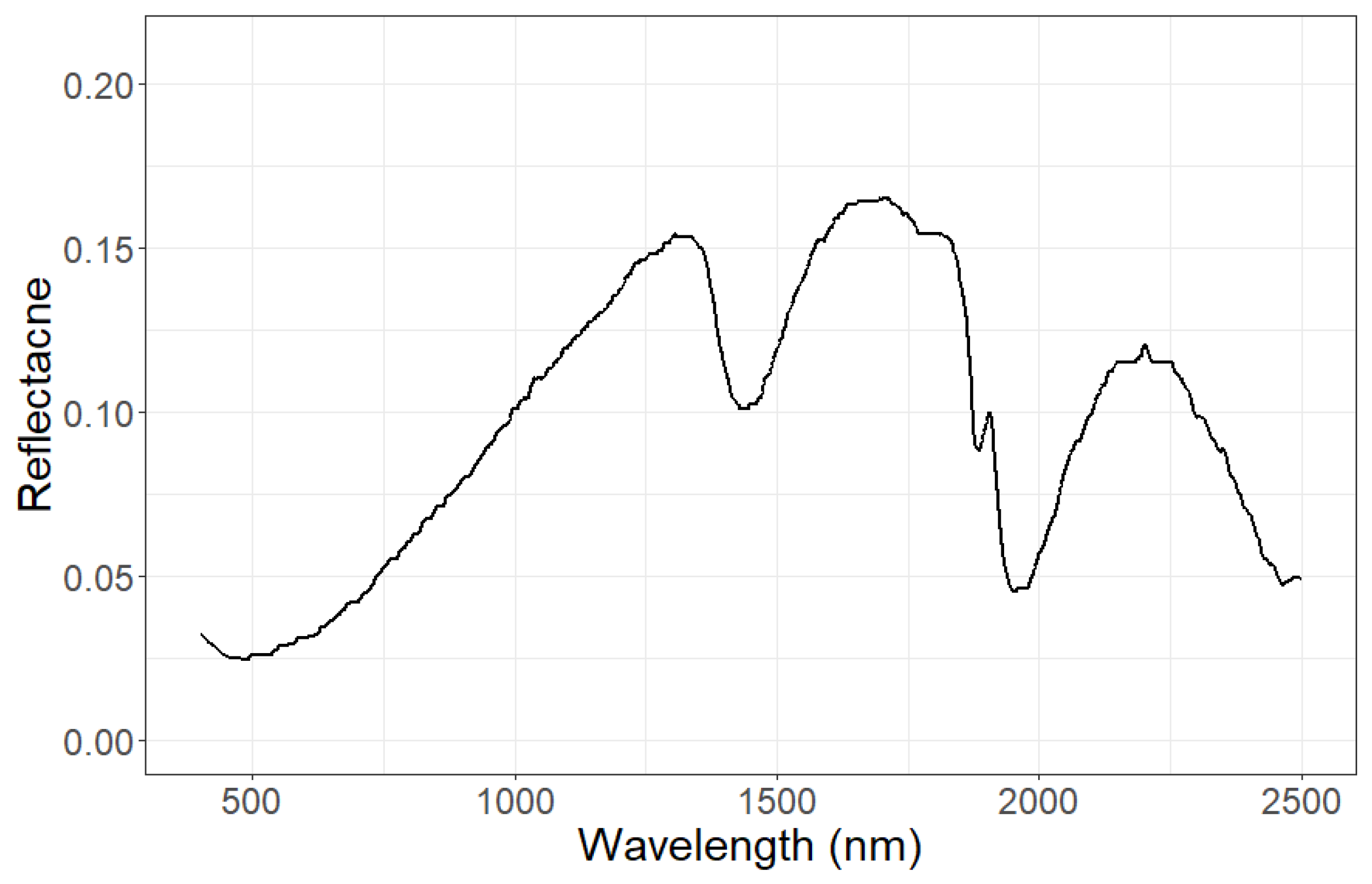

Table A1.
Leaf parameters.
| Leaf parameter | Picea Abies | Pinus Silvestrys | Betula |
|---|---|---|---|
| Cab | |||
| Cdm | |||
| Cw | |||
| Cs | |||
| Car | |||
| N |
Appendix B. Additional information on the result section
Figure A2.
Comparison of reflectance spectra for different layer heights with simple forest representation.
Figure A2.
Comparison of reflectance spectra for different layer heights with simple forest representation.
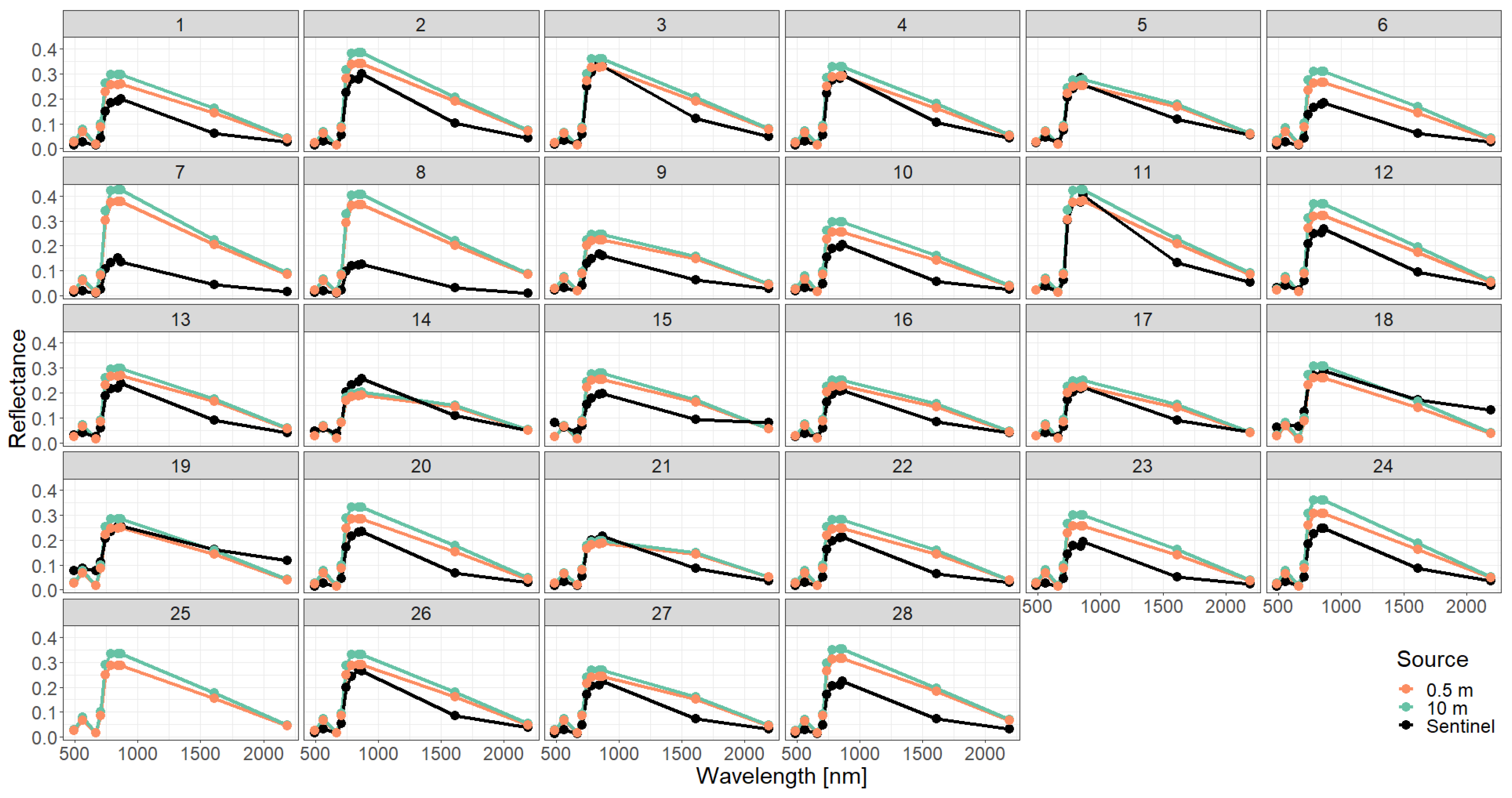
Figure A3.
Comparison of reflectance spectra for different layer heights with detailed forest representation.
Figure A3.
Comparison of reflectance spectra for different layer heights with detailed forest representation.
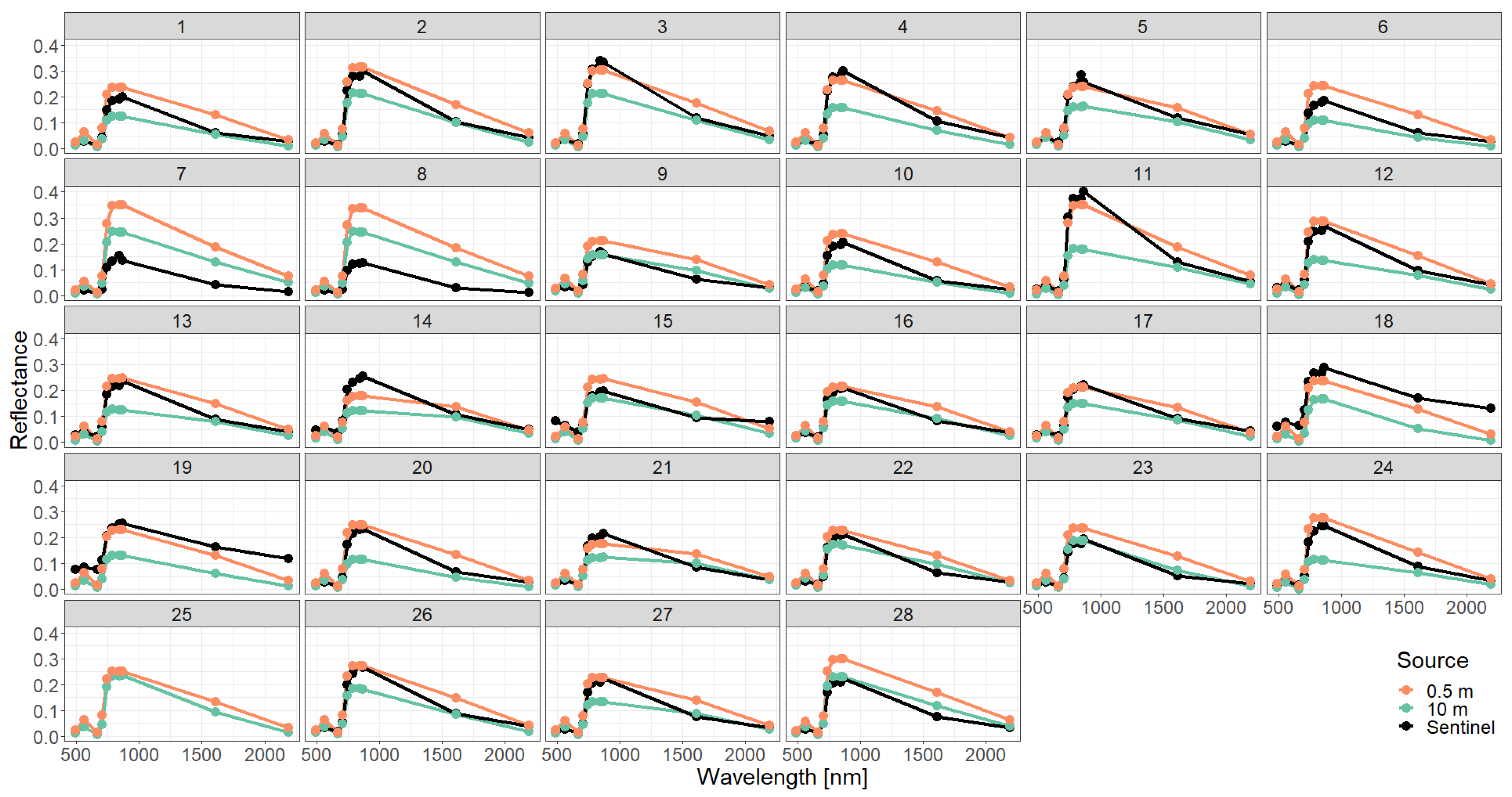
Figure A4.
Comparison of reflectance spectra for different concepts of forest representations with layer height of 10 m.
Figure A4.
Comparison of reflectance spectra for different concepts of forest representations with layer height of 10 m.
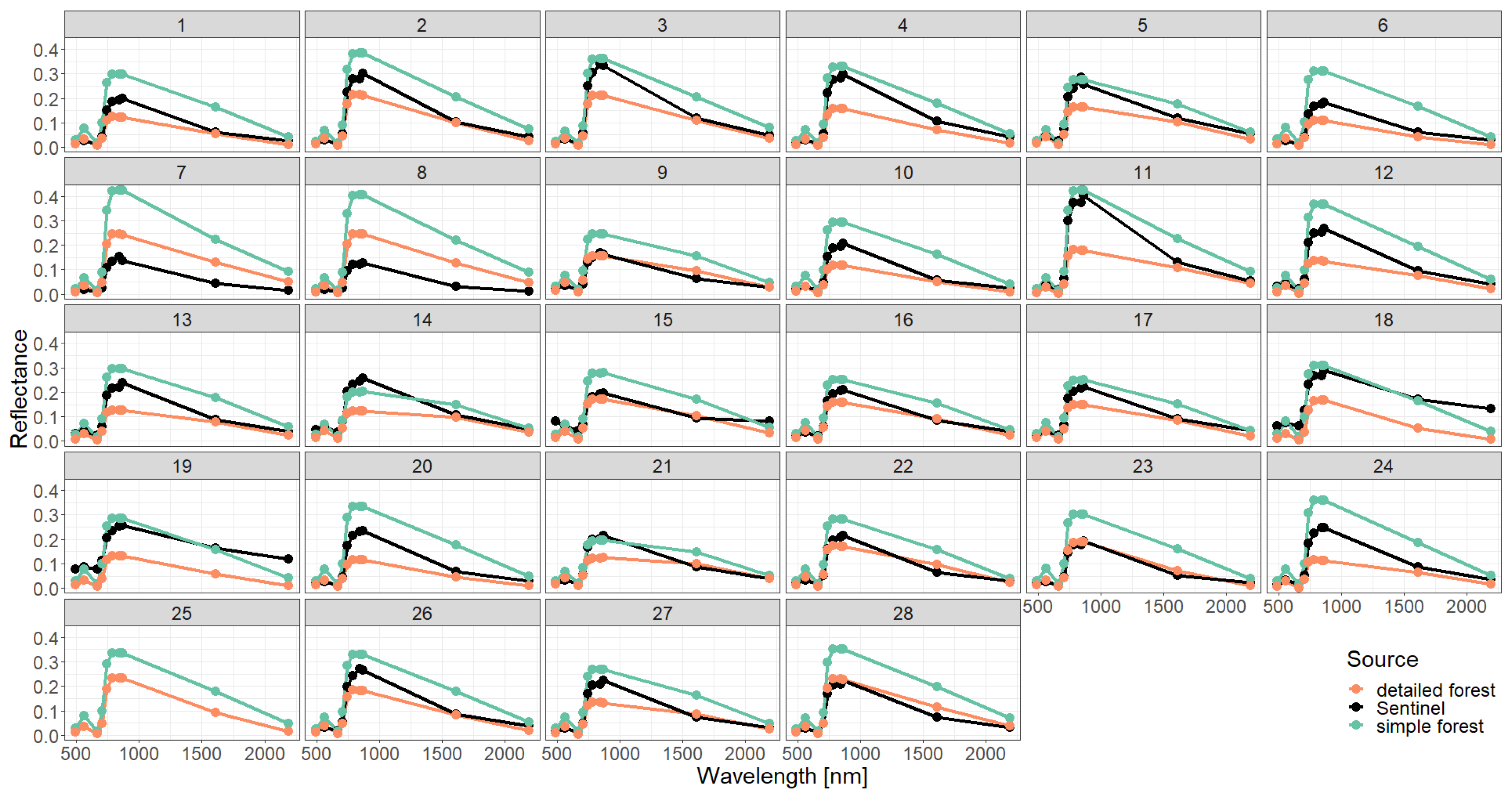
Figure A5.
Comparison of reflectance spectra for different concepts of forest representations with layer height of 0.5 m.
Figure A5.
Comparison of reflectance spectra for different concepts of forest representations with layer height of 0.5 m.
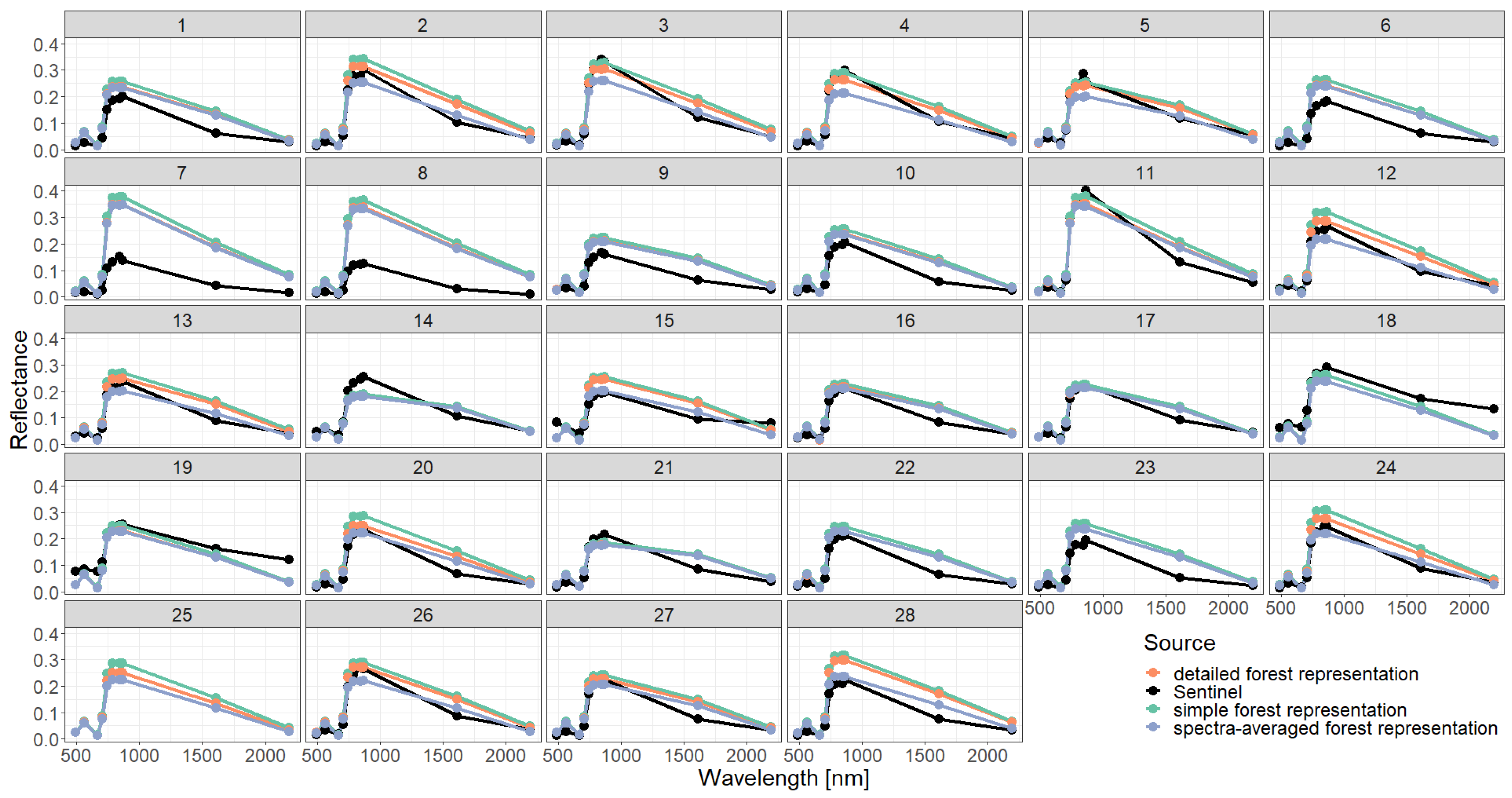
Figure A6.
LAI Profiles for each forest stand. Shown are the LAI values (x-axis) in each height layer (y-axis) per species (red – Betula, green – picea abies, blue - pinus silvestris).
Figure A6.
LAI Profiles for each forest stand. Shown are the LAI values (x-axis) in each height layer (y-axis) per species (red – Betula, green – picea abies, blue - pinus silvestris).
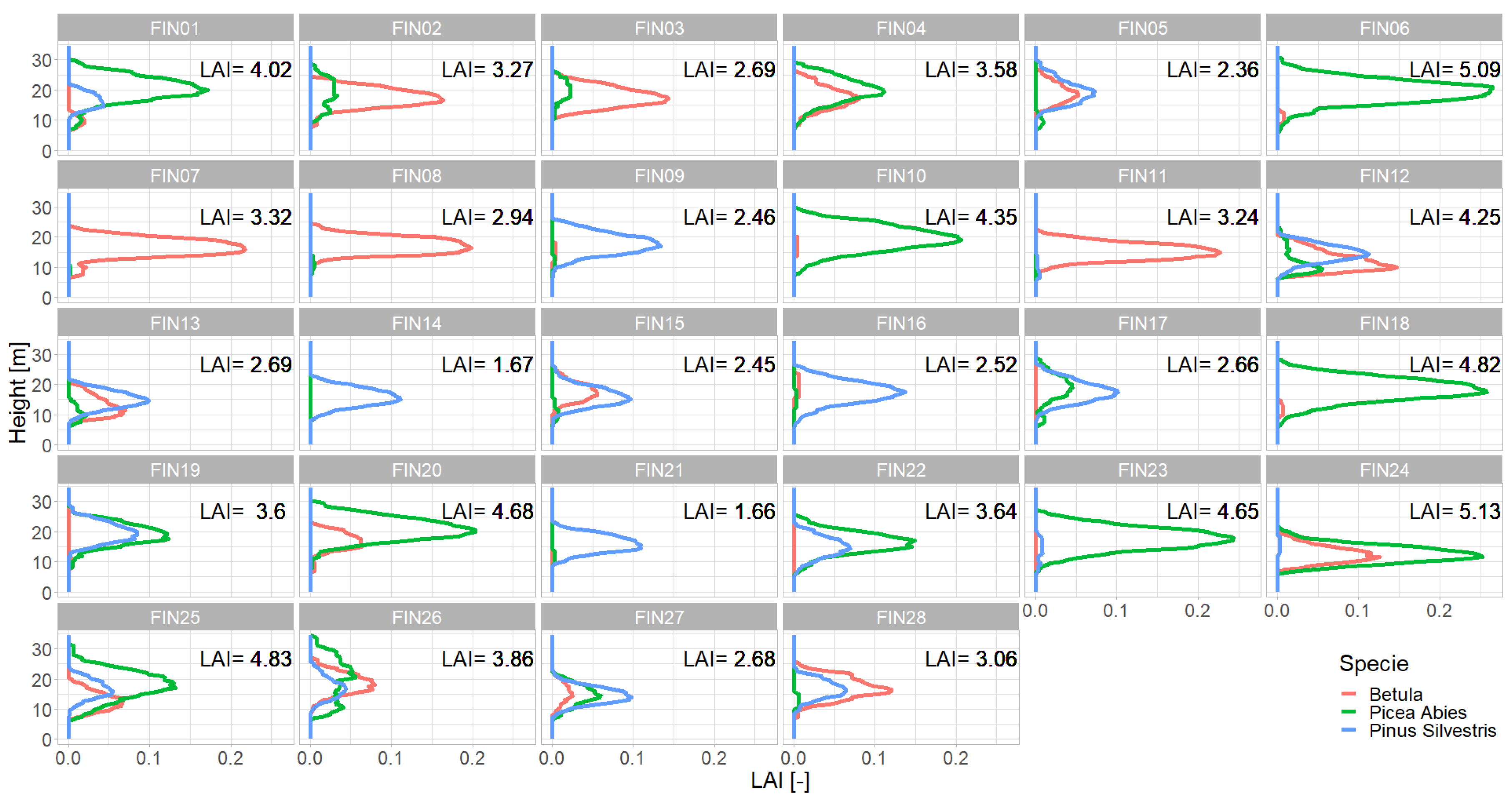
Figure A7.
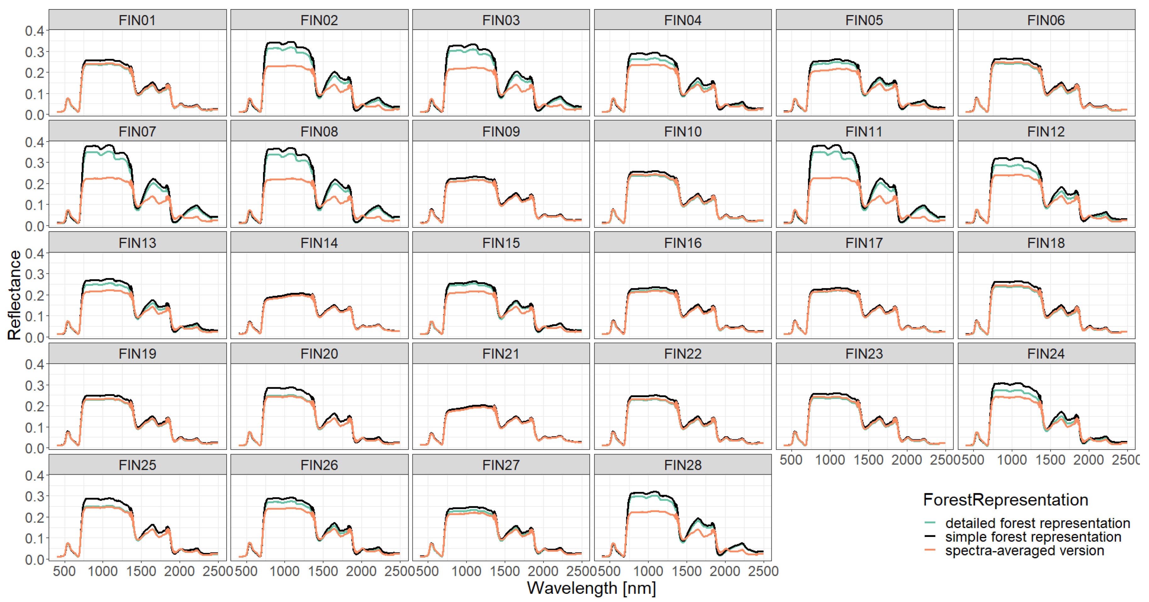
Comparison of reflectance spectra over all wavelength for different concepts of forest representations.
Figure A7.
Comparison of reflectance spectra over all wavelength for different concepts of forest representations.
Appendix C. Analysis of the outliers
Figure A8.
Comparison of reflectance spectra and additional information of forest stand 15 (outlier) with forest stand 5. We compare forest properties of an outlier (left side) with forest properties of a forest with similar attributes, which is not an outlier (right side). Therefore, we compare the LAI profile (outer sides top), the reflectance spectra (in the middle) and the species composition (outer sides bottom). Despite the similar LAI distribution and species composition we see different Sentinel-measurements, but similar simulated reflectance.
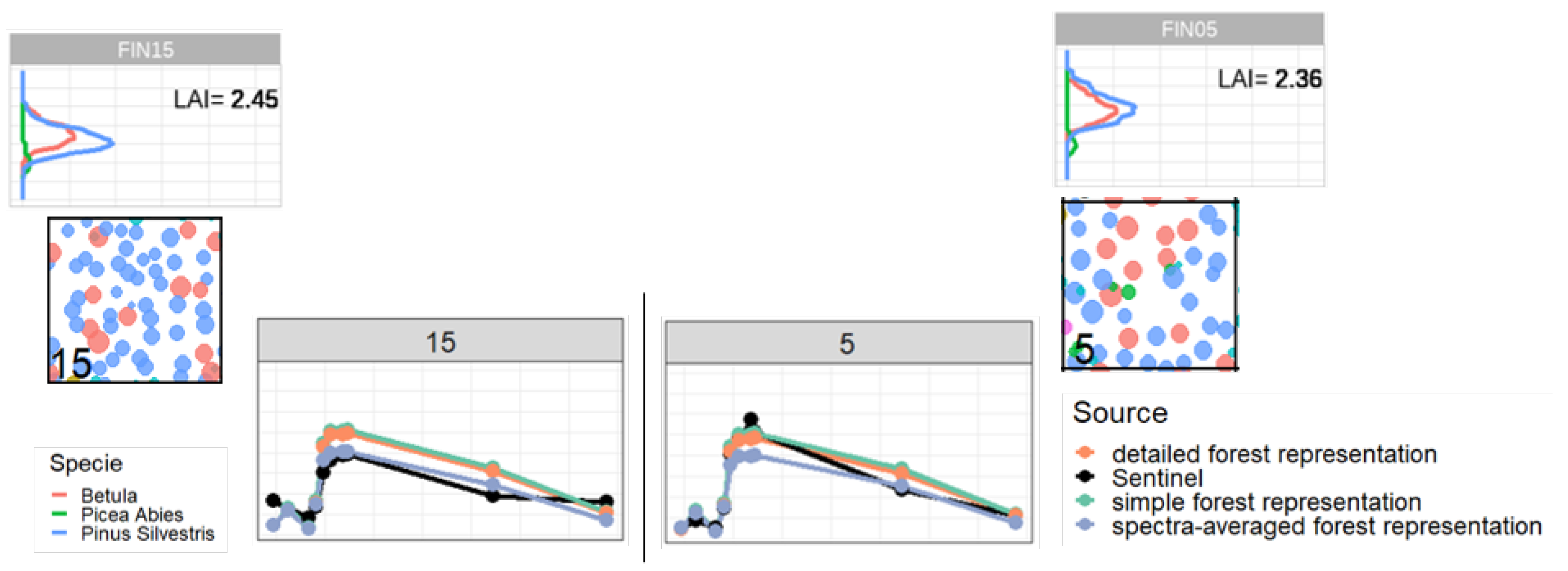
Figure A9.
Comparison of reflectance spectra and additional information of forest stands 7 and 8 (outliers) with forest stand 11. We compare forest properties of two outliers (left side) with forest properties of a forest with similar attributes, which is not an outlier (right side). Therefore, we compare the LAI profile (outer sides top), the reflectance spectra (in the middle) and the species composition (outer sides bottom). Despite the similar LAI distribution and species composition we see different Sentinel-measurements, but similar simulated reflectance.
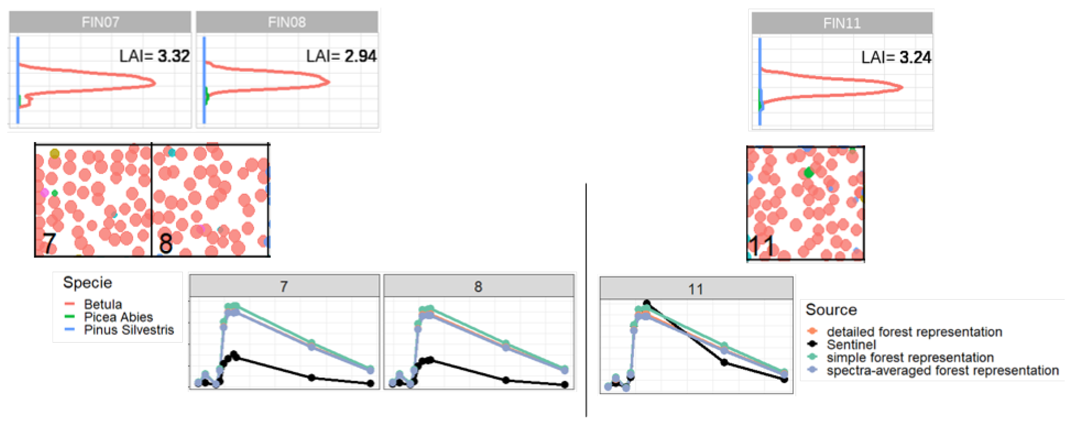
Figure A10.
Comparison of reflectance spectra and additional information of forest stand 19 (outlier) with forest stand 22. We compare forest properties of an outlier (left side) with forest properties of a forest with similar attributes, which is not an outlier (right side). Therefore, we compare the LAI profile (outer sides top), the reflectance spectra (in the middle) and the species composition (outer sides bottom). Despite the similar LAI distribution and species composition we see different Sentinel-measurements, but similar simulated reflectance.
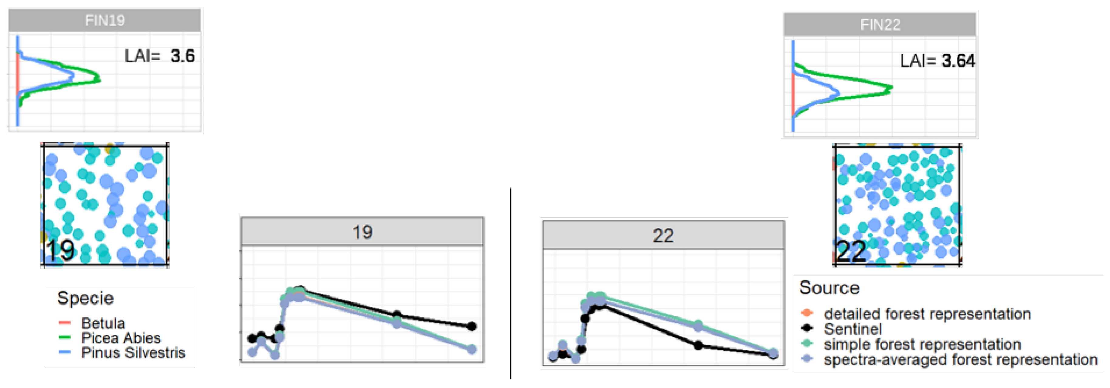
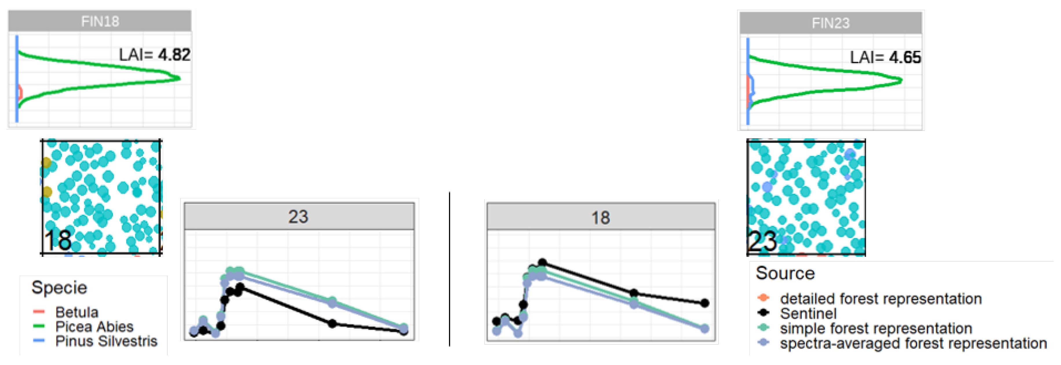
Figure A11.
Comparison of reflectance spectra and additional information of forest stand 18 (outlier) with forest stand 23. We compare forest properties of an outlier (left side) with forest properties of a forest with similar attributes, which is not an outlier (right side). Therefore, we compare the LAI profile (outer sides top), the reflectance spectra (in the middle) and the species composition (outer sides bottom). Despite the similar LAI distribution and species composition we see different Sentinel-measurements, but similar simulated reflectance.
Appendix D. Analysis of LAI and additional indices
Figure A12.
Analysis of the relationship between LAI (x-axis) and NDVI (y-axis) of all Finland forest stands.
Figure A12.
Analysis of the relationship between LAI (x-axis) and NDVI (y-axis) of all Finland forest stands.
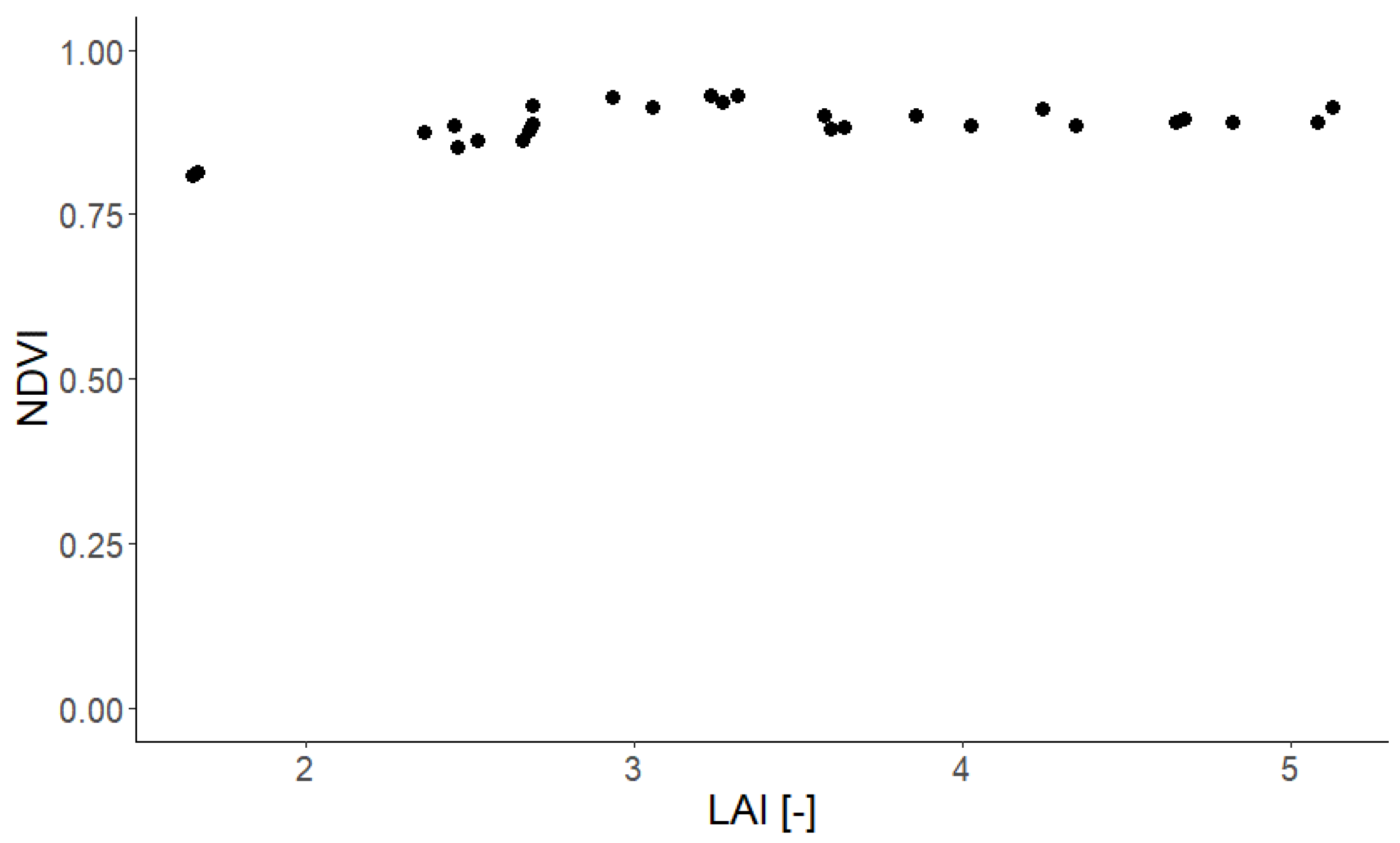
Figure A13.
Comparison of vegetation indices. The vegetation indices (NDMI left, kNDVI right) are calculated from the reflectance values in the different wavebands once for the simulated reflectance spectra (x-axis) and for the satellite measurements (y-axis). In each row, a different forest representation is used to calculate the results of the indices from the simulated spectra (1. detailed forest representation, 2. simple forest representation, 3. spectra-averaged forest representation; more information about the cases in Section 2.2). Each point represents a forest stand in Finland (gray points indicate outliers that are not used to calculate the RMSE and - see Appendix Figure A8, Figure A9, Figure A10 and Figure A11).
References
- Pan, Y.; Birdsey, R.A.; Fang, J.; Houghton, R.; Kauppi, P.E.; Kurz, W.A.; Phillips, O.L.; Shvidenko, A.; Lewis, S.L.; Canadell, J.G.; et al. A Large and Persistent Carbon Sink in the World’s Forests. Science 2011, 333, 988–993. [Google Scholar] [CrossRef] [PubMed]
- Malhi, Y. The carbon balance of tropical forest regions, 1990–2005. Current Opinion in Environmental Sustainability 2010, 2, 237–244. [Google Scholar] [CrossRef]
- Ciais, P.; Sabine, C.L.; Bala, G.; Bopp, L.; Brovkin, V.A.; Canadell, J.G.; Chhabra, A.; DeFries, R.S.; Galloway, J.N.; Heimann, M.; et al. Carbon and Other Biogeochemical Cycles. In Climate Change 2013 – The Physical Science Basis: Working Group I Contribution to the Fifth Assessment Report of the Intergovernmental Panel on Climate Change; Cambridge University Press, 2014; pp. 465–570. [Google Scholar] [CrossRef]
- FAO. The State of the World’s Forests 2022. Forest pathways for green recovery and building inclusive, resilient and sustainable economies. 2022. [Google Scholar] [CrossRef]
- Gibson, L.; Lee, T.M.; Koh, L.P.; Brook, B.W.; Gardner, T.A.; Barlow, J.; Peres, C.A.; Bradshaw, C.J.; Laurance, W.F.; Lovejoy, T.E.; et al. Primary forests are irreplaceable for sustaining tropical biodiversity. Nature 2011, 478, 378–381. [Google Scholar] [CrossRef]
- Myers, N.; Mittermeier, R.A.; Mittermeier, C.G.; Da Fonseca, G.A.; Kent, J. Biodiversity hotspots for conservation priorities. Nature 2000, 403, 853–858. [Google Scholar] [CrossRef] [PubMed]
- Pimm, S.L.; Jenkins, C.N.; Abell, R.; Brooks, T.M.; Gittleman, J.L.; Joppa, L.N.; Raven, P.H.; Roberts, C.M.; Sexton, J.O. The biodiversity of species and their rates of extinction, distribution, and protection. science 2014, 344, 1246752. [Google Scholar] [CrossRef]
- Pan, Y.; Birdsey, R.A.; Phillips, O.L.; Jackson, R.B. The structure, distribution, and biomass of the world’s forests. Annual Review of Ecology, Evolution, and Systematics 2013, 44, 593–622. [Google Scholar] [CrossRef]
- Guanter, L.; Kaufmann, H.; Segl, K.; Foerster, S.; Rogass, C.; Chabrillat, S.; Kuester, T.; Hollstein, A.; Rossner, G.; Chlebek, C.; et al. The EnMAP spaceborne imaging spectroscopy mission for earth observation. Remote Sensing 2015, 7, 8830–8857. [Google Scholar] [CrossRef]
- Moorcroft, P.R.; Hurtt, G.C.; Pacala, S.W. A method for scaling vegetation dynamics: the ecosystem demography model (ED). Ecological monographs 2001, 71, 557–586. [Google Scholar] [CrossRef]
- Lawrence, D.M.; Oleson, K.W.; Flanner, M.G.; Thornton, P.E.; Swenson, S.C.; Lawrence, P.J.; Zeng, X.; Yang, Z.L.; Levis, S.; Sakaguchi, K.; et al. Parameterization improvements and functional and structural advances in version 4 of the Community Land Model. Journal of Advances in Modeling Earth Systems 2011, 3. [Google Scholar] [CrossRef]
- Maréchaux, I.; Langerwisch, F.; Huth, A.; Bugmann, H.; Morin, X.; Reyer, C.P.; Seidl, R.; Collalti, A.; Dantas de Paula, M.; Fischer, R.; et al. Tackling unresolved questions in forest ecology: The past and future role of simulation models. Ecology and Evolution 2021, 11, 3746–3770. [Google Scholar] [CrossRef]
- Shugart, H.H.; Wang, B.; Fischer, R.; Ma, J.; Fang, J.; Yan, X.; Huth, A.; Armstrong, A.H. Gap models and their individual-based relatives in the assessment of the consequences of global change. Environmental Research Letters 2018, 13, 033001. [Google Scholar] [CrossRef]
- Köhler, P.; Huth, A. The effects of tree species grouping in tropical rainforest modelling: Simulations with the individual-based model Formind. Ecological Modelling 1998, 109, 301–321. [Google Scholar] [CrossRef]
- Smith, B. LPJ-GUESS-an ecosystem modelling framework. Department of Physical Geography and Ecosystems Analysis, INES, Sölvegatan 2001, 12, 22362. [Google Scholar]
- Sellers, P.J. Canopy reflectance, photosynthesis and transpiration. International journal of remote sensing 1985, 6, 1335–1372. [Google Scholar] [CrossRef]
- Kokhanovsky, A.A.; Kuusk, A.; Lang, M.; Kuusk, J. Database of optical and structural data for the validation of forest radiative transfer models. Light Scattering Reviews 7: Radiative Transfer and Optical Properties of Atmosphere and Underlying Surface 2013, pp. 109–148. [Google Scholar]
- Kuusk, A. Canopy Radiative Transfer Modeling. In Comprehensive Remote Sensing; Liang, S., Ed.; Elsevier: Oxford, 2018; pp. 9–22. [Google Scholar] [CrossRef]
- Brazhnik, K.; Shugart, H. Model sensitivity to spatial resolution and explicit light representation for simulation of boreal forests in complex terrain. Ecological Modelling 2017, 352, 90–107. [Google Scholar] [CrossRef]
- Deutschmann, T.; Beirle, S.; Frieß, U.; Grzegorski, M.; Kern, C.; Kritten, L.; Platt, U.; Prados-Román, C.; Puķı, J.; Wagner, T.; et al. The Monte Carlo atmospheric radiative transfer model McArtim: Introduction and validation of Jacobians and 3D features. Journal of Quantitative Spectroscopy and Radiative Transfer 2011, 112, 1119–1137. [Google Scholar] [CrossRef]
- Verhoef, W.; Jia, L.; Xiao, Q.; Su, Z. Unified optical-thermal four-stream radiative transfer theory for homogeneous vegetation canopies. IEEE Transactions on geoscience and remote sensing 2007, 45, 1808–1822. [Google Scholar] [CrossRef]
- Bonan, G.B.; Lawrence, P.J.; Oleson, K.W.; Levis, S.; Jung, M.; Reichstein, M.; Lawrence, D.M.; Swenson, S.C. Improving canopy processes in the Community Land Model version 4 (CLM4) using global flux fields empirically inferred from FLUXNET data. Journal of Geophysical Research: Biogeosciences 2011, 116. [Google Scholar] [CrossRef]
- Medvigy, D.; Wofsy, S.; Munger, J.; Hollinger, D.; Moorcroft, P. Mechanistic scaling of ecosystem function and dynamics in space and time: Ecosystem Demography model version 2. Journal of Geophysical Research: Biogeosciences 2009, 114. [Google Scholar] [CrossRef]
- Bonan, G.; Williams, M.; Fisher, R.; Oleson, K. Modeling stomatal conductance in the earth system: linking leaf water-use efficiency and water transport along the soil–plant–atmosphere continuum. Geoscientific Model Development 2014, 7, 2193–2222. [Google Scholar] [CrossRef]
- Gastellu-Etchegorry, J.P.; Lauret, N.; Yin, T.; Landier, L.; Kallel, A.; Malenovský, Z.; Bitar, A.A.; Aval, J.; Benhmida, S.; Qi, J.; et al. DART: Recent Advances in Remote Sensing Data Modeling With Atmosphere, Polarization, and Chlorophyll Fluorescence. IEEE Journal of Selected Topics in Applied Earth Observations and Remote Sensing 2017, 10, 2640–2649. [Google Scholar] [CrossRef]
- Yang, P.; Verhoef, W.; van der Tol, C. The mSCOPE model: A simple adaption to the SCOPE model to describe reflectance, fluorescence and photosynthesis of vertically heterogeneous canopies. Remote Control of Environment 2017, 201, 1–11. [Google Scholar] [CrossRef]
- Köhler, P.; Huth, A. Simulating growth dynamics in a South-East Asian rainforest threatened by recruitment shortage and tree harvesting. Climatic Change 2004, 67, 95–117. [Google Scholar] [CrossRef]
- Gutiérrez, A.G.; Huth, A. Successional stages of primary temperate rainforests of Chiloé Island, Chile. Perspectives in Plant Ecology, Evolution and Systematics 2012, 14, 243–256. [Google Scholar] [CrossRef]
- Huth, A.; Ditzer, T. Long-term impacts of logging in a tropical rain forest—a simulation study. Forest Ecology and management 2001, 142, 33–51. [Google Scholar] [CrossRef]
- Kammesheidt, L.; Köhler, P.; Huth, A. Sustainable timber harvesting in Venezuela: a modelling approach. Journal of applied ecology 2001, 38, 756–770. [Google Scholar] [CrossRef]
- Köhler, P.; Chave, J.; Riéra, B.; Huth, A. Simulating the long-term response of tropical wet forests to fragmentation. Ecosystems 2003, 6, 0114–0128. [Google Scholar] [CrossRef]
- Köhler, P.; Huth, A. Impacts of recruitment limitation and canopy disturbance on tropical tree species richness. ecological modelling 2007, 203, 511–517. [Google Scholar] [CrossRef]
- Rüger, N.; Williams-Linera, G.; Kissling, W.D.; Huth, A. Long-term impacts of fuelwood extraction on a tropical montane cloud forest. Ecosystems 2008, 11, 868–881. [Google Scholar] [CrossRef]
- Fischer, R.; Armstrong, A.; Shugart, H.H.; Huth, A. Simulating the impacts of reduced rainfall on carbon stocks and net ecosystem exchange in a tropical forest. Environmental modelling & software 2014, 52, 200–206. [Google Scholar]
- Rödig, E.; Cuntz, M.; Rammig, A.; Fischer, R.; Taubert, F.; Huth, A. The importance of forest structure for carbon fluxes of the Amazon rainforest. Environmental Research Letters 2018, 13, 054013. [Google Scholar] [CrossRef]
- Bohn, F.J.; Frank, K.; Huth, A. Of climate and its resulting tree growth: Simulating the productivity of temperate forests. Ecological Modelling 2014, 278, 9–17. [Google Scholar] [CrossRef]
- Bruening, J.M.; Fischer, R.; Bohn, F.J.; Armston, J.; Armstrong, A.H.; Knapp, N.; Tang, H.; Huth, A.; Dubayah, R. Challenges to aboveground biomass prediction from waveform lidar. Environmental Research Letters 2021, 16, 125013. [Google Scholar] [CrossRef]
- Rüger, N.; Gutiérrez, A.G.; Kissling, W.D.; Armesto, J.J.; Huth, A. Ecological impacts of different harvesting scenarios for temperate evergreen rain forest in southern Chile—a simulation experiment. Forest Ecology and Management 2007, 252, 52–66. [Google Scholar] [CrossRef]
- Taubert, F.; Frank, K.; Huth, A. A review of grassland models in the biofuel context. Ecological Modelling 2012, 245, 84–93. [Google Scholar] [CrossRef]
- Reyer, C.P.O.; Silveyra Gonzalez, R.; Dolos, K.; Hartig, F.; Hauf, Y.; Noack, M.; Lasch-Born, P.; Rötzer, T.; Pretzsch, H.; Meesenburg, H.; et al. The PROFOUND Database for evaluating vegetation models and simulating climate impacts on European forests. Earth System Science Data 2020, 12, 1295–1320. [Google Scholar] [CrossRef]
- Paulick, S.; Dislich, C.; Homeier, J.; Fischer, R.; Huth, A. The carbon fluxes in different successional stages: modelling the dynamics of tropical montane forests in South Ecuador. Forest Ecosystems 2017, 4, 1–11. [Google Scholar] [CrossRef]
- Baeten, L.; Verheyen, K.; Wirth, C.; Bruelheide, H.; Bussotti, F.; Finér, L.; Jaroszewicz, B.; Selvi, F.; Valladares, F.; Allan, E.; et al. A novel comparative research platform designed to determine the functional significance of tree species diversity in European forests. Perspectives in Plant Ecology, Evolution and Systematics 2013, 15, 281–291. [Google Scholar] [CrossRef]
- Ma, X.; Mahecha, M.D.; Migliavacca, M.; van der Plas, F.; Benavides, R.; Ratcliffe, S.; Kattge, J.; Richter, R.; Musavi, T.; Baeten, L.; et al. Inferring plant functional diversity from space: the potential of Sentinel-2. Remote Sensing of Environment 2019, 233, 111368. [Google Scholar] [CrossRef]
- van der Tol, C.; Verhoef, W.; Timmermans, J.; Verhoef, A.; Su, Z. An integrated model of soil-canopy spectral radiances, photosynthesis, fluorescence, temperature and energy balance. Biogeosciences 2009, 6, 3109–3129. [Google Scholar] [CrossRef]
- Féret, J.B.; Gitelson, A.; Noble, S.; Jacquemoud, S. PROSPECT-D: Towards modeling leaf optical properties through a complete lifecycle. Remote Sensing of Environment 2017, 193, 204–215. [Google Scholar] [CrossRef]
- Kothari, S.; Beauchamp-Rioux, R.; Blanchard, F.; Crofts, A.L.; Girard, A.; Guilbeault-Mayers, X.; Hacker, P.W.; Pardo, J.; Schweiger, A.K.; Demers-Thibeault, S.; et al. Predicting leaf traits across functional groups using reflectance spectroscopy. New Phytologist 2023, 238, 549–566. [Google Scholar] [CrossRef]
- Huete, A.; Didan, K.; Miura, T.; Rodriguez, E.P.; Gao, X.; Ferreira, L.G. Overview of the radiometric and biophysical performance of the MODIS vegetation indices. Remote sensing of environment 2002, 83, 195–213. [Google Scholar] [CrossRef]
- Gao, X.; Huete, A.R.; Ni, W.; Miura, T. Optical–biophysical relationships of vegetation spectra without background contamination. Remote sensing of environment 2000, 74, 609–620. [Google Scholar] [CrossRef]
- Camps-Valls, G.; Campos-Taberner, M.; Álvaro, Moreno-Martínez.; Walther, S.; Duveiller, G.; Cescatti, A.; Mahecha, M.D.; Muñoz-Marí, J.; García-Haro, F.J.; Guanter, L.; et al. A unified vegetation index for quantifying the terrestrial biosphere. Science Advances 2021, 7, eabc7447. [Google Scholar] [CrossRef]
- Hardisky, M.H.; Klemas, V.; Smart, R. The influence of soil salinity, growth form, and leaf moisture on-the spectral radiance of Spartina alterniflora Canopies. Photogramm. Eng. Remote Sens 1983, 49, 77–83. [Google Scholar]
- Hunt Jr, E.R.; Rock, B.N. Detection of changes in leaf water content using near-and middle-infrared reflectances. Remote sensing of environment 1989, 30, 43–54. [Google Scholar] [CrossRef]
- Vogelmann, J.; Rock, B. Assessing forest decline in coniferous forests of Vermont using NS-001 Thematic Mapper Simulator data. International Journal of Remote Sensing 1986, 7, 1303–1321. [Google Scholar] [CrossRef]
- Huete, A.R.; Liu, H.; Batchily, K.; van Leeuwen, W. A comparison of vegetation indices over a global set of TM images for EOS-MODIS. Remote Sensing of Environment 1997, 59, 440–451. [Google Scholar] [CrossRef]
- Bussotti, F.; Pollastrini, M. Evaluation of leaf features in forest trees: Methods, techniques, obtainable information and limits. Ecological indicators 2015, 52, 219–230. [Google Scholar] [CrossRef]
- Jacquemoud, S.; Ustin, S. Leaf optical properties. Cambridge University Press, 2019. [Google Scholar]
- Kattenborn, T.; Fassnacht, F.E.; Schmidtlein, S. Differentiating plant functional types using reflectance: which traits make the difference? Remote Sensing in Ecology and Conservation 2019, 5, 5–19. [Google Scholar] [CrossRef]
- Kattenborn, T.; Richter, R.; Guimarães-Steinicke, C.; Feilhauer, H.; Wirth, C. AngleCam: Predicting the temporal variation of leaf angle distributions from image series with deep learning. Methods in Ecology and Evolution 2022, 13, 2531–2545. [Google Scholar] [CrossRef]
- Jacquemoud, S.; Verhoef, W.; Baret, F.; Bacour, C.; Zarco-Tejada, P.J.; Asner, G.P.; François, C.; Ustin, S.L. PROSPECT+ SAIL models: A review of use for vegetation characterization. Remote sensing of environment 2009, 113, S56–S66. [Google Scholar] [CrossRef]
- Verhoef, W.; Van Der Tol, C.; Middleton, E.M. Hyperspectral radiative transfer modeling to explore the combined retrieval of biophysical parameters and canopy fluorescence from FLEX–Sentinel-3 tandem mission multi-sensor data. Remote sensing of environment 2018, 204, 942–963. [Google Scholar] [CrossRef]
- Rödig, E.; Knapp, N.; Fischer, R.; Bohn, F.J.; Dubayah, R.; Tang, H.; Huth, A. From small-scale forest structure to Amazon-wide carbon estimates. Nature communications 2019, 10, 5088. [Google Scholar] [CrossRef]
- Henniger, H.; Huth, A.; Frank, K.; Bohn, F. Creating virtual forest around the globe: Forest Factory 2.0 and analysing the state space of forests. Ecological Modelling 2023. [Google Scholar] [CrossRef]
- Bohn, F.J.; Huth, A. The importance of forest structure to biodiversity–productivity relationships. Royal Society open science 2017, 4, 160521. [Google Scholar] [CrossRef]
- Pacheco-Labrador, J.; Perez-Priego, O.; El-Madany, T.S.; Julitta, T.; Rossini, M.; Guan, J.; Moreno, G.; Carvalhais, N.; Martín, M.P.; Gonzalez-Cascon, R.; et al. Multiple-constraint inversion of SCOPE. Evaluating the potential of GPP and SIF for the retrieval of plant functional traits. Remote Sensing of Environment 2019, 234, 111362. [Google Scholar] [CrossRef]
- Fischer, R.; Bohn, F.; Dantas de Paula, M.; Dislich, C.; Groeneveld, J.; Gutiérrez, A.G.; Kazmierczak, M.; Knapp, N.; Lehmann, S.; Paulick, S.; et al. Lessons learned from applying a forest gap model to understand ecosystem and carbon dynamics of complex tropical forests. Ecological Modelling 2016, 326, 124–133. [Google Scholar] [CrossRef]
Figure 1.
Visualisation of the forest inventory of the 28 forest stands in Finland (reconstruction of 2015). Each circle represents a tree located by its x and y coordinates (X and Y axis). The color of the circles represents the species of a tree and the size of the circle represents its crown diameter. The number in the squares indicates the number of the forest stand. The forest stands are shown the side by side.
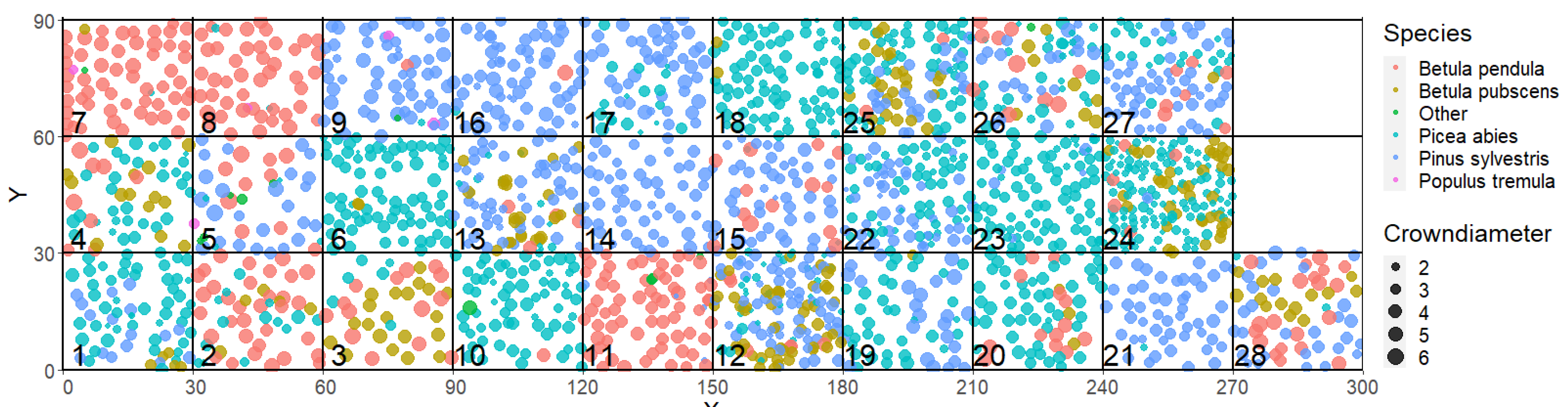
Figure 2.
Different concepts of forest representation Visualization of the different representations of a sample forest during the simulation (1st column: Simple forest representation, 2nd column: detailed forest representation, 3rd column: spectra-averaged forest representation). We see how, under the given concept, the forest is represented in FORMIND (1st row), how it is simulated in mScope (2nd row) and how the output is built (3rd row). The sample forest has 3 different species (represented by the different colours). The concepts of representation are described in detail in the text.
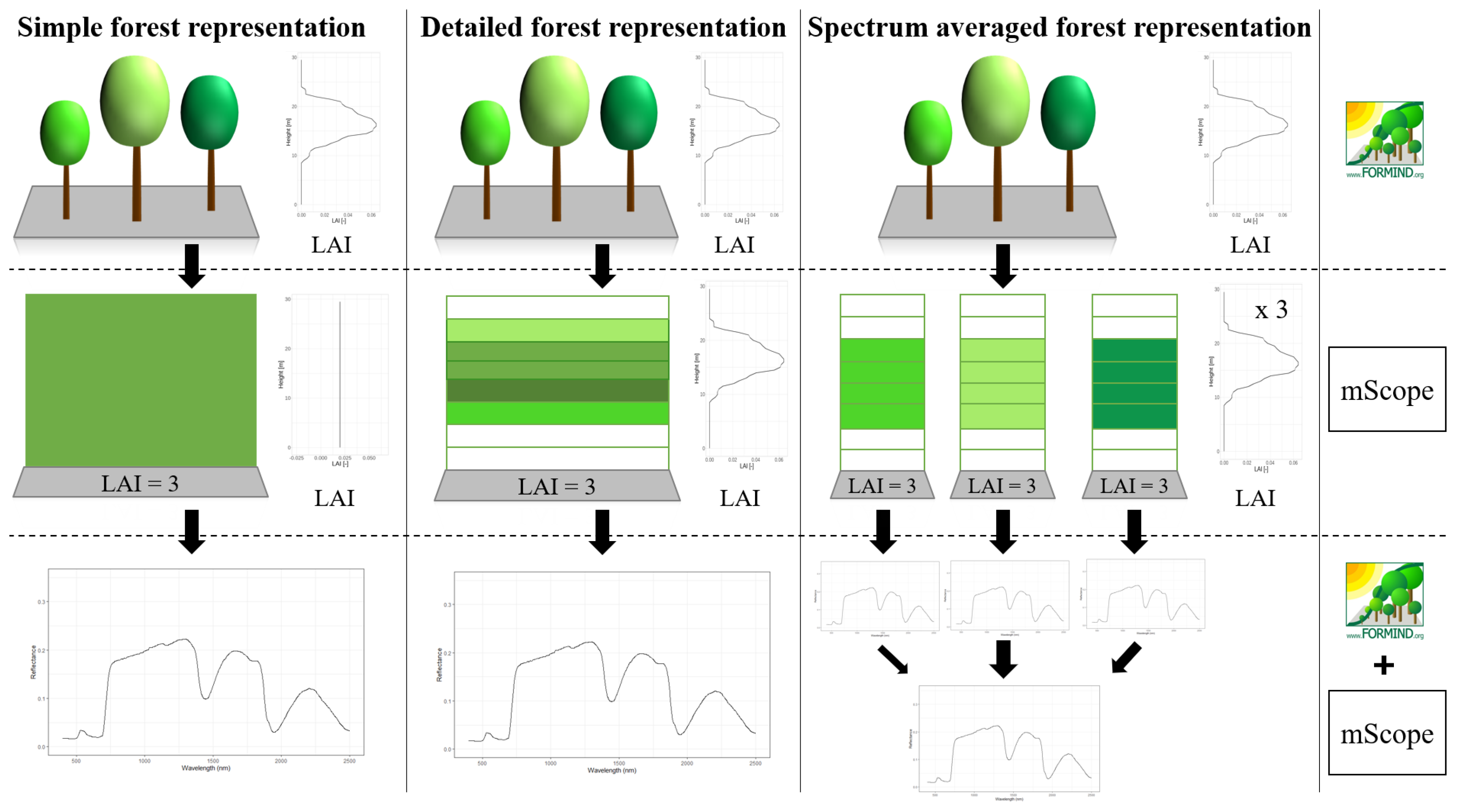
Figure 4.
Reflectance spectra for detailed and simplified forest representation by using standard layers of 0.5 m height. Visualization of the calculated reflectance profiles for two forest stands (no. 5 and 17) in Finland according to Figure 2 is shown. Each point represents the averaged reflectance value over the specific bands (corresponding to the bands of Sentinel-2). Sentinel measurements are shown in black and simulated reflectance is shown in orange/blue from coupling a forest model (FORMIND) with mScope. We use here 0.5 m height layers. The reflection of all other forest stands is shown in the Appendix (Figure A5) Additionally, the reflection for the complete spectra of all other forest stands is shown in the Appendix (Figure A7).
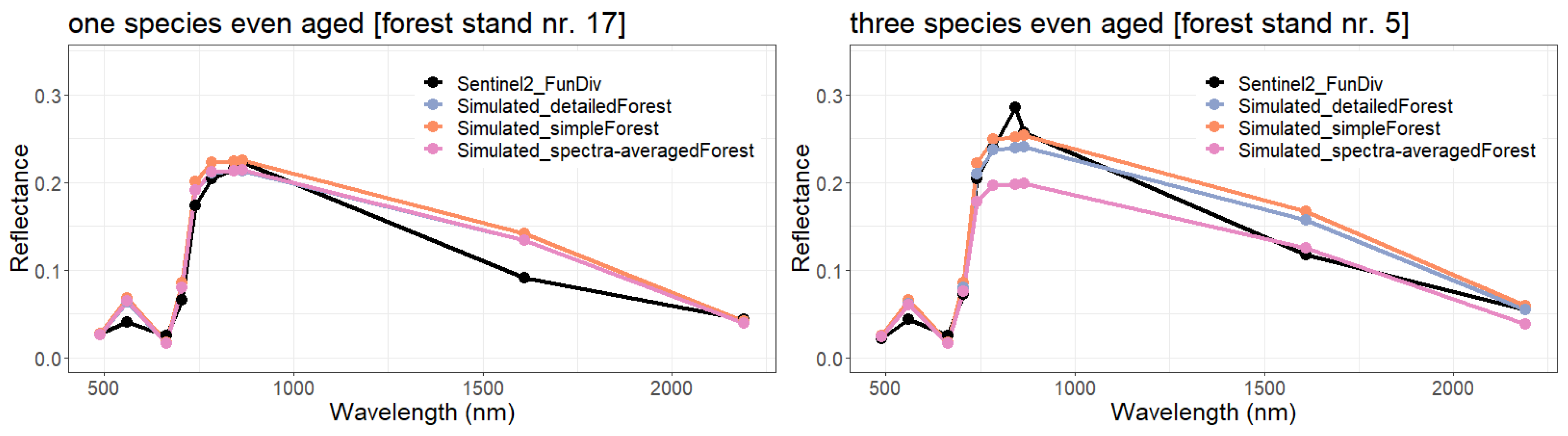
Figure 5.
Comparison of vegetation indices. The vegetation indices (NDVI left, EVI middle, MSI right) are calculated from the reflectance values in the different wavebands once for the simulated reflectance spectra (x-axis) and for the satellite measurements (y-axis). In each row, a different forest representation is used to calculate the results of the indices from the simulated spectra (1. detailed forest representation, 2. simple forest representation, 3. spectra-averaged forest representation; more information about the cases in Section 2.2). Each point represents a forest stand in Finland (gray points indicate outliers that are not used to calculate the RMSE and - see Appendix Figure A8, Figure A9, Figure A10 and Figure A11). Results for the calculation of the NDMI and the KNDVI can be found in the Appendix (Figure A13).
Disclaimer/Publisher’s Note: The statements, opinions and data contained in all publications are solely those of the individual author(s) and contributor(s) and not of MDPI and/or the editor(s). MDPI and/or the editor(s) disclaim responsibility for any injury to people or property resulting from any ideas, methods, instructions or products referred to in the content. |
© 2023 by the authors. Licensee MDPI, Basel, Switzerland. This article is an open access article distributed under the terms and conditions of the Creative Commons Attribution (CC BY) license (http://creativecommons.org/licenses/by/4.0/).
Copyright: This open access article is published under a Creative Commons CC BY 4.0 license, which permit the free download, distribution, and reuse, provided that the author and preprint are cited in any reuse.


