
Submitted:
07 May 2023
Posted:
08 May 2023
You are already at the latest version
Abstract
Activated sludge process is a well known method to treat municipal and industrial waste water. In this complex process, the oxygen concentration in the reactors plays a critical role in the plant efficiency. This paper proposes the use of a Long Short-Term Memory (LSTM) network to identify an input-output model suitable for the design of an oxygen concentration controller. The model is identified from easy-accessible measures collected from a real plant. This dataset covers almost a month. The performances achieved with the proposed LSTM model are compared with the ones obtained with a standard AutoRegressive model with eXogenous input (ARX). Both models catch the oscillation and the overall behaviour (ARX ρ=0.833 , LSTM ρ=0.921), but, while the ARX model fails in reaching the correct amplitude (FIT=41.20%), the LSTM presents satisfactory performance (FIT=60.56%).
Keywords:
Black-box models
; Neural networks
; LSTM
; oxygen concentration modeling
1. Introduction
A WasteWater Treatment Plant (WWTP) is a plant where the wastewater is treated to remove pollutants, exploiting biological and chemical reactions before being released back to the environment. The modeling and control of this process is not trivial, since the treatment depends on the nature and the characteristics of the wastewater. Wastewater usually firstly undergoes to chemical-physical treatments, in order to remove the solid part of the wastes, and then to biological treatments for the organic components. One of the most common biological treatment used in WWTPs is the Conventional Activated Sludge (CAS) process, where bacteria are used to nitrify and denitrify wastewater.
Considering the complexity of the process, the control of a WWTP can be a challenging task: several flows may be involved, among with a huge variety of different biological and chemical reactions; it is necessary to provide a sufficient oxygen quantity but without an excess of aeration, reaching a trade-off between energy consumption and process demand, with a growing attention to the environmental related problems. To design an optimal control strategy it is necessary to have an accurate model of the process [1]. In [2] a review on the current state of the art regarding modeling of activated sludge WWTPs is presented.
The model of the entire WWTP is usually composed by two main components: the hydraulic model that takes into account the different flows in input and output in the reactor, and the Activated Sludge Model (ASM) that models the biological and chemical reactions inside the tank due to the activated sludge process. The so called Activated Sludge Model No. 1 (ASM1) [3] was extended in the years to consider the phosphorus dynamics in ASM2 [4] and including storage of organic substrates as a new process with an easier calibration in ASM3 [5]. Anyway, ASM1 is still the most used model and it can be considered the state of the art since several successive works are based on it [6,7,8]. However, complex and specialized models require the identification of more specific parameters subject to high sensitivity, with expensive and time consuming procedures, far from practical applications. Hence, these specialized models are not a good choice for process design and practical applications and in [9] the combination of the process knowledge with new artificial intelligence techniques is proposed. Also in [2], in addition to the most diffused WWTP white-box modeling, some black-box methodologies based on Neural Network (NN) techniques were presented with interesting results.
In view of all these considerations, in this work a NN approach is explored to model a WWTP located in Mortara (Pavia, Italy), managed by the company ASMortara S.p.A.. The main goal was the development of a model for the biological reactor of the plant to improve several critical aspects of the process such as the oxygen concentration regulation. The data used in this paper, in fact, have been collected with a simple switching controller enabling (disabling) the input flow if the oxygen concentration inside the reactor is below (above) a certain threshold. The effect of this control strategy is an on/off oxygen flow rate, that generates important oscillations in the oxygen concentration evolution.
2. Materials and Methods
This work is focused on modeling the dynamic of the oxygen in the reactor. In the physical models ASM1, ASM2, ASM3, the oxygen concentration (output), , is mainly connected to few manipulable variables (input): the inlet flow of the wastewater, , and its Chemical Oxygen Demand, (); the oxygen inlet flow, ; the outlet flow of the clarified liquid filtered by the membrane, and the one manually removed, .
Even if this notion is general, as clearly stated in the Introduction, every plant has its own peculiarity due to the local law limit, the design constraint, the average chemical composition of the waste and other factors [10]. This fact should require a model identification that is typically impossible in view of the limited number of variables measurable on a real plant. Black-box models, and in particular NN, can be a reasonable compromise to overcome this limitation.
In the following, the plant in hand is described in details; then, the proposed Long Short-Term Memory (LSTM) is reported and compared with a classic AutoRegressive model with eXogenous input (ARX).
2.1. Plant description
The considered WWTP is an industrial plant actually used to treat both municipal and industrial wastewater. The plant is composed by two different units (see Figure 1) dedicated to the two stages of the treatment, called primary and secondary.
The industrial wastewater needs to be pre-treated before being accepted in municipal WWTP: it passes in Unit I to remove the solid part of the waste, exploiting chemical reactions. Firstly, the flow goes into a storage-equalization tank, with the goal to transform a variable flow into a steady-state one that goes in input to the treatment plant, optimizing in this way the process. The flow is then divided in two chemical-physical treatment lines: one dedicated to the light strength aqueous wastes and the second for the high strength ones. The light strength wastes are subjected to a chemical-physical treatment with classic procedures like flocculation, coagulation and sedimentation. The wastes are put in sedimentation tanks where the solid part is separated by gravity; chemicals can be added to help coagulation, while with flocculation the small colloidal particles are separated from the wastes and settle in form of flocks. The high strength aqueous waste instead are fed into a Thermophilic Aerobic Membrane Reactor (TAMR). The plant has been recently equipped with this innovative reactor, built ad-hoc to treat high strength wastes. The advantages of the TAMR technology is the exploiting of biological reactions even during the pre-treating phase, considering that biological solutions are more affordable and sustainable of chemical ones. In practice, the waste undergoes to aerobic reactions in thermophilic conditions, exploiting oxygen with temperatures greater than 45 °C [12,13].
After this phase, the pre-treated industrial wastewater is mixed with the municipal wastewater and flow into the biological reactor (Unit II), where the CAS comprehends denitrification (DEN), oxidation and nitrification (OX-NIT). This paper is focus on the modelling of this part of the plant. The biological reactor is filled with oxygen, where aerobic microorganisms are introduced to react with wastewater and to reduce its organic compounds. The overall flow goes to a settling tank (Final settler) where the activated sludge settles, since the micro-organisms create a biological flock, producing a liquid mostly free from suspended solid. The sludge is separated from the clarified water: the majority of the sludge is reintroduced in the CAS to treat the new wastewater, the remaining part is removed, while the cleared water is released in the environment. In the biological reactor the wastewater is subjected also to the denitrification and nitrification processes to remove the nitrogen components from the wastewater. This is done before releasing back the water in the environment since these components are dangerous for aquatic organisms and plants. The nitrification occurs in aerobic conditions and is the oxidation of ammonia into nitrite and nitrate by nitrifying autotrophic bacteria; the denitrification instead happens in anaerobic conditions to reduce nitrite to nitrogen [14]. For this reason nitrate recirculates from OX-NIT to DEN (Figure 1).
2.2. Long Short-Term Memory (LSTM) network
The LSTM [15,16] is a particular type of Recurrent Neural Network (RNN), that thanks to its specific units architecture, called memory cells, is able to learn the information dependencies better than a simpler RNN. The LSTM memory cell presents an internal self-loop, in addition to the outer feedback present in all the RNNs, and a gating system that regulates the flow of information. In this way, the gradient flows during time, even for long periods, and its derivative do not explode nor vanish.
The mathematical formulation of a single memory cell is represented in Figure 2 and can be expressed as follows:
where is the internal cell state at time k, is the input at time k and is the hidden state at time k, with n the cell state dimension, that corresponds to the number of LSTM neurons, m the number of features/input of the LSTM, × is the Hadamard product and is the hyperbolic tangent, used as activation function.
Four structures, called gates, regulates the internal loop of the cell adding or removing information to modify the value of the cell state at each time instant. The first gate is the forget gate, , that decides which information is removed from the cell state , multiplying it by its past value , as can be seen in the first part of (1a). Then the input gate, , chooses which value of the cell state is updated, while the input activation gate, , creates a new candidate value of the cell state. The last gate is the output gate, , that determines which information contained in the cell state is going in output. The hidden state is then defined in (), where the output gate is multiplied by a transformation of the cell state through hyperbolic tangent function. These gates are expressed as:
where , , , are the input weight matrices, , , , are the previous output weight matrices and are the biases. These quantities are specific of each gate and identified during the training of the network. The chosen activation functions are the hyperbolic tangent and , the sigmoid function, equal to:
Several LSTM cells are combined in the so-called LSTM layer and the LSTM network can be composed by one or more stacked layers, representing the hidden layers. In regression applications, usually, the output of the last (if more) LSTM layer is passed to a fully connected layer without activation function, that computes a linear combination, according to the following equation:
where is the matrix of the output weights, with p the number of outputs of the network, and the bias. and are determined during the training of the network as well.
Thanks to this structure, LSTMs show their strength especially when dealing with temporal data and when temporal lags must be taken into account [16,17,18,19,20]. The LSTM developed in this work considers 3 inputs (): the ingoing oxygen flow rate , the ingoing substrate flow rate and the outgoing liquid substrate flow rate , and one output (), the oxygen concentration . In this case the other inputs of the physical process and are not considered in input since they are daily measurements, with very little variations, that can be considered almost constant signals not significantly contributing to the model. All the signals have been rescaled using mean normalization before being used to train the LSTM network.
2.3. AutoRegressive model with eXogenous input (ARX) Model
The ARX model family is the most used model structure to derive input-output models. According to this family [21], the process output y is given by three component: the autoregressive component (the previous value of the output), the exogenous input variable, u, and a white Gaussian addictive noise, e. The process output can be defined as
where the suffix k indicates the time k of the sample, and are the order of the autoregressives and of the input component respectively, and d is the input delay; those values as a whole are commonly addressed as the structure of the ARX model. In this scenario the one step predictor is given by the following
where the prediction is obtained using also the last output values (). For MISO systems, the former equation is usually provided in the following compact notation
where M is the number of inputs, is the m-th input discrete signal at time k, , are polynomial in terms of the time-shift operator and is the delay for the m-th input.
To estimate polynomial models, input delays and model orders have to be defined. If the physics of the system is known, the number of poles and zeros can be set accordingly. However, in most cases, the model orders are not known in advance. In those cases, the identification of an ARX model is a three steps procedure [21]: first the data have to be conditioned, then the structure of the model (i.e. polynomial’s degrees and input delays) has to be identified, and finally the parameters (i.e. the polynomial’s coefficients) have to be estimated.
In control design, the models are commonly used to simulate the behavior of the process, so that the previous outputs are not available. Hence, the final predictions will be obtained using the ARX model as
in order to be compared with the LSTM ones (eq. 4).
2.3.1. Data conditioning
In order to identify a linear approximation around the working point of the system [22], a common precondition techniques involves the use of the deviation with respect to the working point instead of the regular signal. The signal average values are used to approximate the plant working point. Hence, the signals in hand become:
where and are the average value of the output and of the m-th input signal. Then, the ARX model predictor became:
2.3.2. Model structure estimation
To get initial model orders and delays for the system, several ARX models can be estimated within a range of orders and delays, then the performance of these models can be compared. So, the model orders that correspond to the best model performance are selected and used as an initial guess for the next phase.
To guarantee a fair comparison to models having different degrees of freedom, a simple validation is used [23]. According to this techniques the data are split into two sets: identification and validation. Each model is identified using the first set while the performance of the model are evaluated on the second set. Then, the best model structure is the one minimising the prediction error computed on the validation data set.
The ASM model family [3,4,5] has been used to determine the ranges of the desired structure parameters. According to those models, the number of states ranges from 12 to 15, no delay is involved and the proposed model is strictly proper. Starting from this consideration, the parameter space was determined. The main idea is that the research space has to include the structure proposed by the physical models. In particular, the degree of is connected to the order of the system then it was supposed , and for each input the sum delay and order should also include the same limit, . Table 1 summarizes the proposed ranges.
2.3.3. Parameter estimation
This final phase is devoted to determine the model. The structure is now known, so the whole dataset can now be used to determine the best model. Moreover, this work aim to identify a model of a real plant which is intrinsically stable [3]. Then, the stability is enforced. From a mathematical point of view, this can be view as:
where is set of the -degree Hurwitz polynomial.
2.4. Datasets description
The WWTP is monitored through a Supervisory Control And Data Acquisition (SCADA) system used to manage the control protocols, alarm handling and also for data collection. From the SCADA interface the user can have access to sensors equipped in the chemical-physical reactor (where the wastewater is pre-treated), in the biological reactor and in the two membrane bioreactors, called respectively MBR1 and MBR2.
In this way, the signals of interest can be downloaded. The value of is obtained from the chemical-physical reactor, from which it goes in input into the biological reactor, after the preprocessing of the wastewater. In the reactor are then present sensors that measure the ingoing oxygen flow rate, , the oxygen concentration, , measured at a height of 4 meters. Then, the measure of the output liquid substrate flow rate, , is obtained from MBR1 and MBR2, as the sum of the two components that from the biological reactor flow into the two membrane bioreactors.
Lastly, is obtained through laboratory analysis as well as that is acquired daily by the operators who remove it from the reactor. These quantities are not considered in the models, not only for their constant values, but also for the difficulty in their acquisition.
Six different datasets are collected, each one containing six days of data, as in Table 2. All the datasets contain the three inputs and the output previously described. Dataset 1 is used as testing dataset, while the remaining 5 datasets are used to train and validate the models.
2.5. Performance Indexes
Three performance indexes are considered:
- Index of fitting (): normalized index that indicates how much the prediction matches the real data. For a perfect prediction it is equal to 100% and it can also be negative. It is expressed as:
- Pearson correlation coefficient (): it measures the linear correlation between two variables and has a value between -1 (total negative correlation) and +1 (total positive correlation).
- Root Mean Squared Error (): it shows the Euclidean distance of the predictions from the real data using.
where y is the vector of the real data, of the predicted ones, containing S elements each, and , are their respective mean values.
The training and validation of the models are performed on five datasets (Dataset 2 - Dataset 6) for a total amount of thirty days, while it is tested on the remaining one, Dataset 1.
3. Results
Due to privacy compliance, the working point of the plant is not made fully available: only the oxygen concentration is showed and available as full data (). This choice preserves the privacy of the company that provided them, and allows a complete comparison of the results.
The performance of the two approaches will be presented individually, and compared in the next Sections.
3.1. LSTM results
The LSTM network presents an architecture composed by a single layer LSTM with 160 neurons, trained for 1000 epochs, using Adam optimizer with learning rate and Mean Squared Error (MSE) loss function defined as:
The values of the hyperparameters have been obtained through an optimization procedure with KerasTuner [24], employing the algorithm with the number of neurons spanning in the range [32; 512] and the learning rate in [0.001; 0.01].
The training of the network is performed on a computer Intel i9-10920X CPU with 3.50 GHz, with graphics processing unit GPU NVIDIA GeForce RTX 2080Ti; it has been written in Python 3.9, using TensorFlow [25], Keras API [26] and KerasTuner [24]. The results are quite satisfying, with , and . An example of the prediction obtained with the LSTM is reported in Figure 3, with a global overview in Figure 3 and a closer detail of the first 12 hours in Figure 3, to better emphasize the accuracy of the result. It can be observed that both the global dynamic of the signal and the oscillations are correctly reproduced, with an overall satisfying outcome.
3.2. ARX
The procedure described in Section 2.3 was conducted using the System Identification Toolbox of Matlab [27].
Table 1 (last column) reports the structures of the model selected by the procedure.
The identified model was used to simulate the testing dataset. Figure 4 shows the comparison between the actual oxygen concentration and the predicted one. The oscillation frequencies and the overall behaviour are correctly estimated (), but the model fails in reaching the correct amplitude ( and ). Those results are emphasized in the zoom reported in Figure 4 and summarized by the performance indicators.
3.3. Discussion
The performance indexes are reported in Table 3 for both the presented techniques.
In Figure 5 a zoomed graph of the comparison of the two techniques is presented. It is evident how the LSTM is able to better follow the peaks while the ARX model underestimates in particular the maximum values.
4. Conclusions
This work proposes the use of a LSTM network to identify an input-output model suitable for the design of an oxygen concentration controller in an Activated Sludge process to treat municipal and industrial waste water. The model is identified using easy-accessible measures collected from a real plant located in Mortara, Italy. The LSTM showed satisfactory performances being able to catch both the oscillation and the overall behaviour ( and ). It also overcomes the performance of a classic ARX ( and ) which is not able to reach the correct amplitude.
The design of a controller based on the LSTM presented in this work is proposed as future development of this work.
Author Contributions
Conceptualization, C.T. and L.M.; methodology, C.T., F.D.P., F.I. and L.M. ; software, F.D.P. and F.I.; validation, C.T., F.D.P. and F.I.; formal analysis, C.T. and F.D.P.; resources, L.M.; data curation, F.D.P. and F.I.; writing—original draft preparation, C.T., F.D.P. and F.I.; writing—review and editing, C.T., F.D.P. and L.M.; supervision, C.T. and L.M.; project administration, L.M..; funding acquisition, L.M.. All authors have read and agreed to the published version of the manuscript.
Funding
This research was funded by Azienda Servizi Mortara S.p.A..
Data Availability Statement
Data available in a publicly accessible repository at https://arxiv.org//XXXX.
Conflicts of Interest
The authors declare no conflict of interest.
Abbreviations
The following abbreviations are used in this manuscript:
| ASM1 | Activated Sludge Model No. 1 |
| ASM2 | Activated Sludge Model No. 2 |
| ASM3 | Activated Sludge Model No. 3 |
| ARX | AutoRegressive eXogenous |
| CAS | Conventional Activated Sludge |
| COD | Chemical Oxygen Demand |
| DEN | Denitrification |
| LSTM | Long Short-Term Memory |
| MSE | Mean Squared Error |
| NN | Neural Network |
| OX-NIT | Oxidation and nitrification |
| RMSE | Root Mean Squared Error |
| RNN | Recurrent Neural Network |
| SCADA | Supervisory Control And Data Acquisition |
| TAMR | Thermophilic Aerobic Membrane Reactor |
| WWTP | WasteWater Treatment Plant |
References
- Hamitlon, R.; Braun, B.; Dare, R.; Koopman, B.; Svoronos, S.A. Control issues and challenges in wastewater treatment plants. IEEE control systems magazine 2006, 26, 63–69. [Google Scholar]
- Gernaey, K.V.; Van Loosdrecht, M.C.; Henze, M.; Lind, M.; Jørgensen, S.B. Activated sludge wastewater treatment plant modelling and simulation: state of the art. Environmental modelling & software 2004, 19, 763–783. [Google Scholar]
- Henze, M.; Grady Jr, C.L.; Gujer, W.; Marais, G.; Matsuo, T. A general model for single-sludge wastewater treatment systems. Water Research 1987, 21, 505–515. [Google Scholar] [CrossRef]
- Gujer, W.; Henze, M.; Mino, T.; Matsuo, T.; Wentzel, M.; Marais, G. The Activated Sludge Model No. 2: Biological phosphorus removal. Water Science and Technology 1995, 31, 1–11, Modelling and Control of Activated Sludge Processes. [Google Scholar] [CrossRef]
- Gujer, W.; Henze, M.; Mino, T.; Van Loosdrecht, M. Activated sludge model No. 3. Water Science and Technology 1999, 39, 183–193, Modelling and microbiology of activated sludge processes. [Google Scholar] [CrossRef]
- Nelson, M.; Sidhu, H.S. Analysis of the activated sludge model (number 1). Applied Mathematics Letters 2009, 22, 629–635. [Google Scholar] [CrossRef]
- Nelson, M.; Sidhu, H.S.; Watt, S.; Hai, F.I. Performance analysis of the activated sludge model (number 1). Food and Bioproducts Processing 2019, 116, 41–53. [Google Scholar] [CrossRef]
- Gujer, W. Activated sludge modelling: past, present and future. Water Science and Technology 2006, 53, 111–119. [Google Scholar] [CrossRef] [PubMed]
- Sin, G.; Al, R. Activated sludge models at the crossroad of artificial intelligence—A perspective on advancing process modeling. Npj Clean Water 2021, 4, 1–7. [Google Scholar] [CrossRef]
- Hreiz, R.; Latifi, M.; Roche, N. Optimal design and operation of activated sludge processes: State-of-the-art. Chemical Engineering Journal 2015, 281, 900–920. [Google Scholar] [CrossRef]
- Collivignarelli, M.C.; Abbà, A.; Bertanza, G.; Setti, M.; Barbieri, G.; Frattarola, A. Integrating novel (thermophilic aerobic membrane reactor-TAMR) and conventional (conventional activated sludge-CAS) biological processes for the treatment of high strength aqueous wastes. Bioresource technology 2018, 255, 213–219. [Google Scholar] [CrossRef] [PubMed]
- Collivignarelli, M.; Abbà, A.; Frattarola, A.; Manenti, S.; Todeschini, S.; Bertanza, G.; Pedrazzani, R. Treatment of aqueous wastes by means of Thermophilic Aerobic Membrane Reactor (TAMR) and nanofiltration (NF): Process auditing of a full-scale plant. Environmental monitoring and assessment 2019, 191, 1–17. [Google Scholar] [CrossRef] [PubMed]
- Collivignarelli, M.C.; Abbà, A.; Bertanza, G. Why use a thermophilic aerobic membrane reactor for the treatment of industrial wastewater/liquid waste? Environmental Technology 2015, 36, 2115–2124. [Google Scholar] [CrossRef] [PubMed]
- Frącz, P. Nonlinear modeling of activated sludge process using the Hammerstein-Wiener structure. In Proceedings of the E3S Web of Conferences. EDP Sciences; 2016; Vol. 10, p. 00119. [Google Scholar]
- Hochreiter, S.; Schmidhuber, J. Long short-term memory. Neural computation 1997, 9, 1735–1780. [Google Scholar] [CrossRef] [PubMed]
- Gers, F.A.; Schmidhuber, J.; Cummins, F. Learning to forget: Continual prediction with LSTM. Neural computation 2000, 12, 2451–2471. [Google Scholar] [CrossRef] [PubMed]
- Gers, F.A.; Schraudolph, N.N.; Schmidhuber, J. Learning precise timing with LSTM recurrent networks. Journal of machine learning research 2002, 3, 115–143. [Google Scholar]
- Pascanu, R.; Mikolov, T.; Bengio, Y. On the difficulty of training recurrent neural networks. In Proceedings of the International conference on machine learning. PMLR; 2013; pp. 1310–1318. [Google Scholar]
- Greff, K.; Srivastava, R.K.; Koutník, J.; Steunebrink, B.R.; Schmidhuber, J. LSTM: A search space odyssey. IEEE transactions on neural networks and learning systems 2016, 28, 2222–2232. [Google Scholar] [CrossRef] [PubMed]
- Pham, V.; Bluche, T.; Kermorvant, C.; Louradour, J. Dropout improves recurrent neural networks for handwriting recognition. In Proceedings of the 2014 14th international conference on frontiers in handwriting recognition. IEEE; 2014; pp. 285–290. [Google Scholar]
- Ljung, L. (Ed.) System Identification (): Theory for the User, 2Nd Ed.; Prentice Hall PTR: Upper Saddle River, NJ, USA, 1999. [Google Scholar]
- Söderström, T.; Stoica, P. System Identification; Prentice Hall PTR: Upper Saddle River, NJ, USA, 1989. [Google Scholar]
- Godfrey, K. Correlation methods. Automatica 1980, 16, 527–534. [Google Scholar] [CrossRef]
- O’Malley, T.; Bursztein, E.; Long, J.; Chollet, F.; Jin, H.; Invernizzi, L.; et al. KerasTuner. https://github.com/keras-team/keras-tuner, 2019.
- Abadi, M.; Agarwal, A.; Barham, P.; Brevdo, E.; Chen, Z.; Citro, C.; Corrado, G.S.; Davis, A.; Dean, J.; Devin, M.; et al. TensorFlow: Large-Scale Machine Learning on Heterogeneous Systems, 2015. Software available from tensorflow.org.
- Chollet, F.; et al. Keras. https://keras.io, 2015.
- The MathWorks Inc., Natick, Massachusetts, United States. System Identification Toolbox version: 9.16 (R2022a), 2022.
Figure 1.
Flow diagram of the WWTP [11].
Figure 1.
Flow diagram of the WWTP [11].
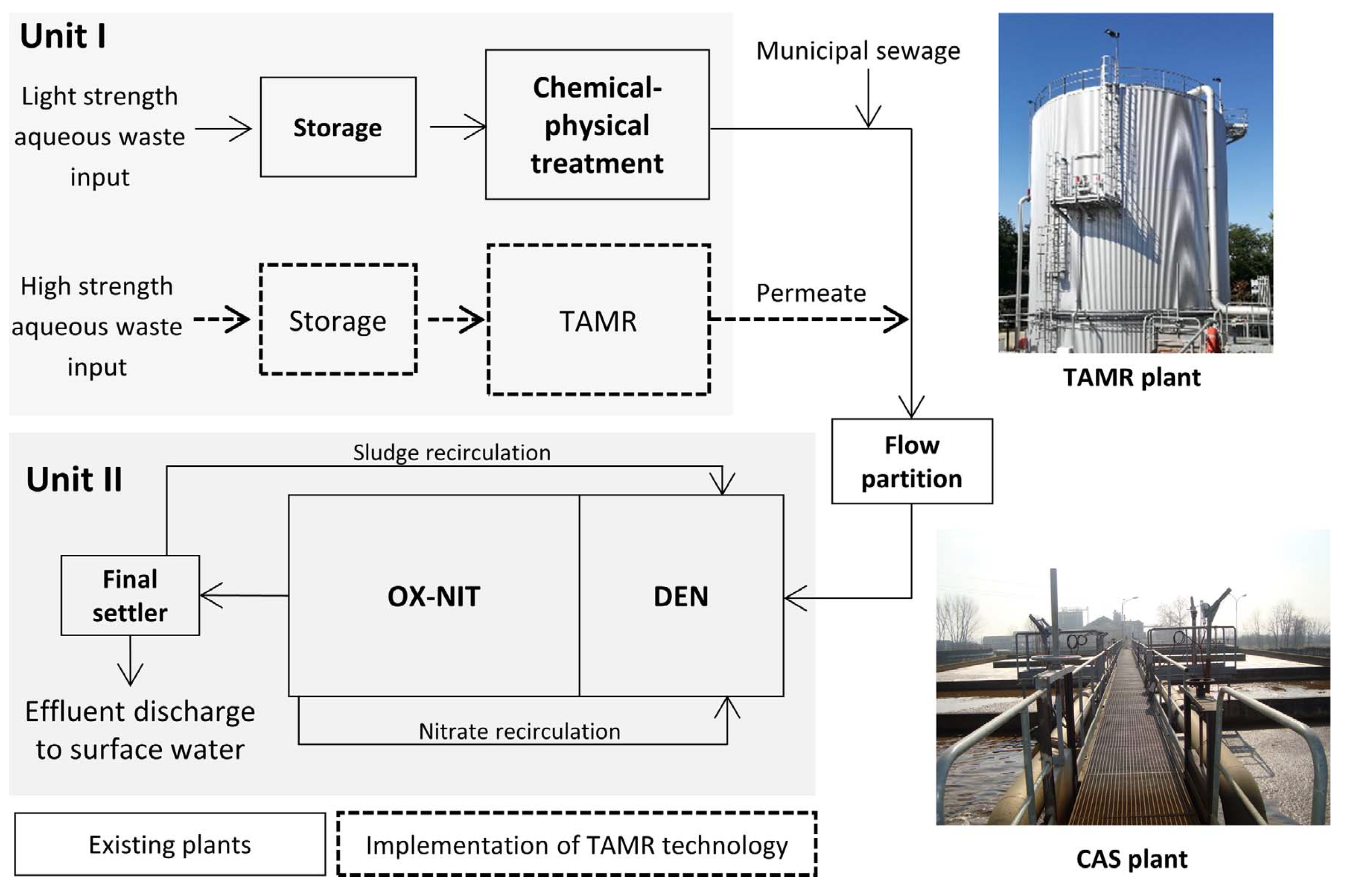
Figure 2.
Scheme of a single LSTM cell.
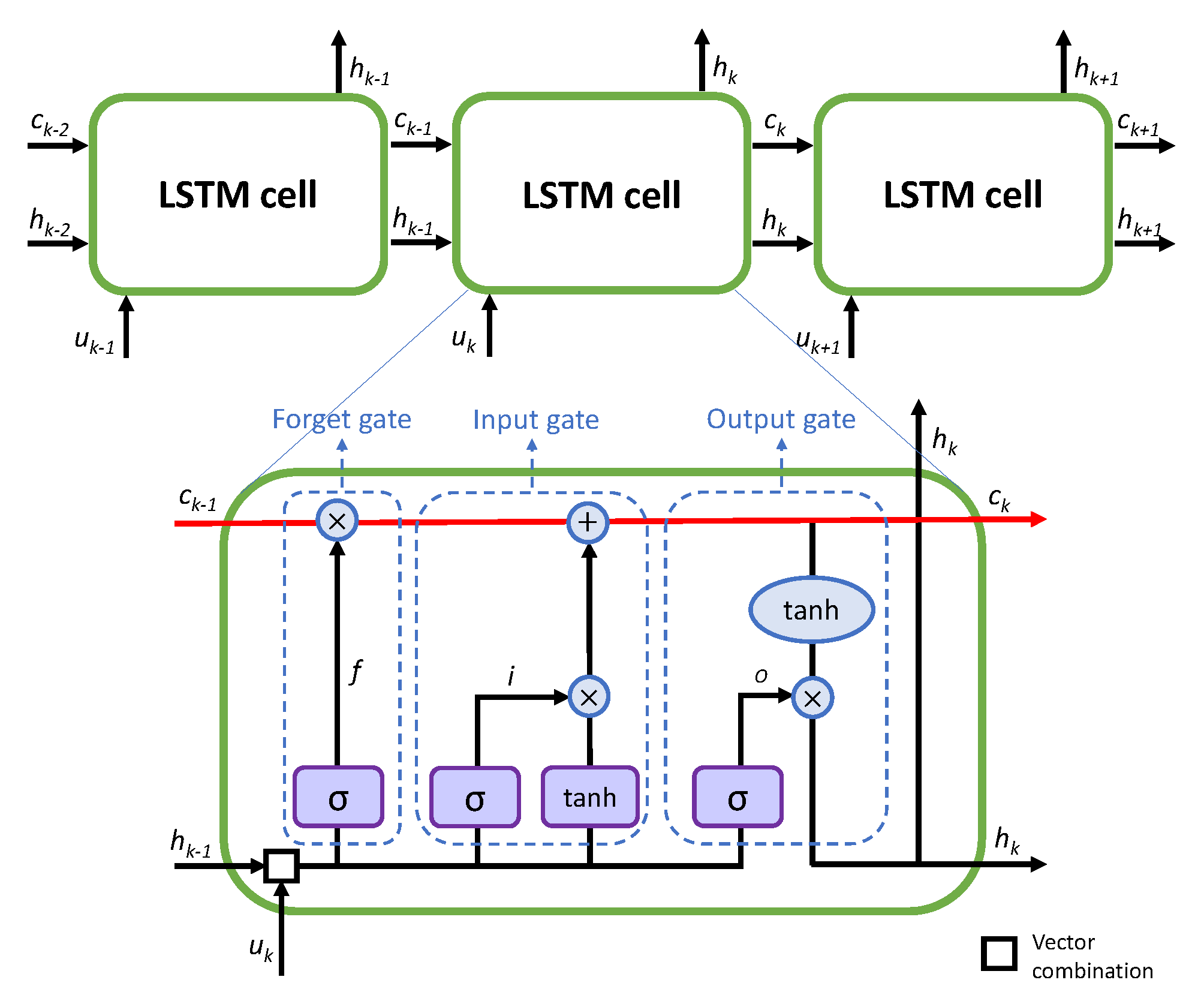
Figure 3.
Results of the LSTM model.
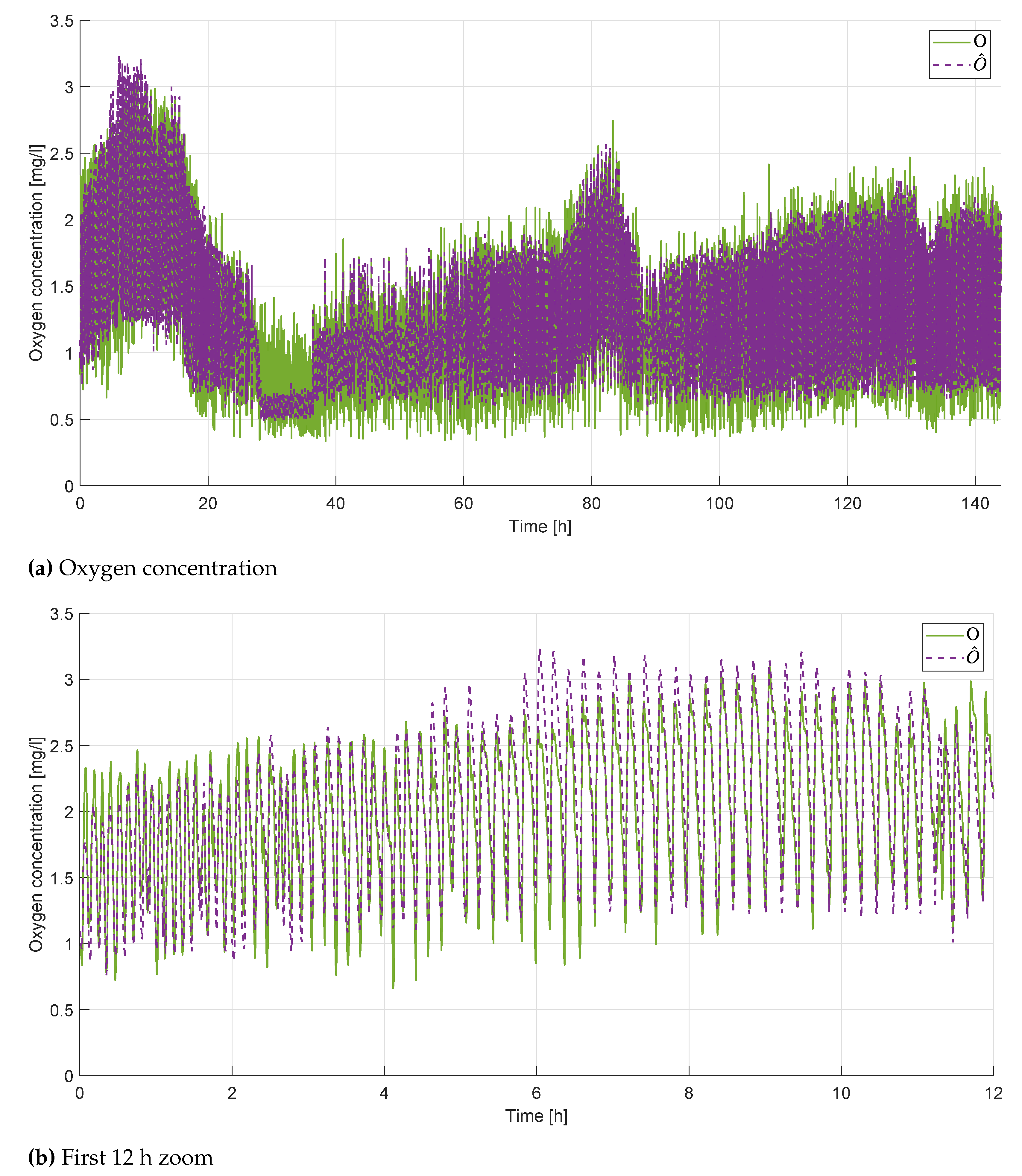
Figure 4.
Results of the ARX model.
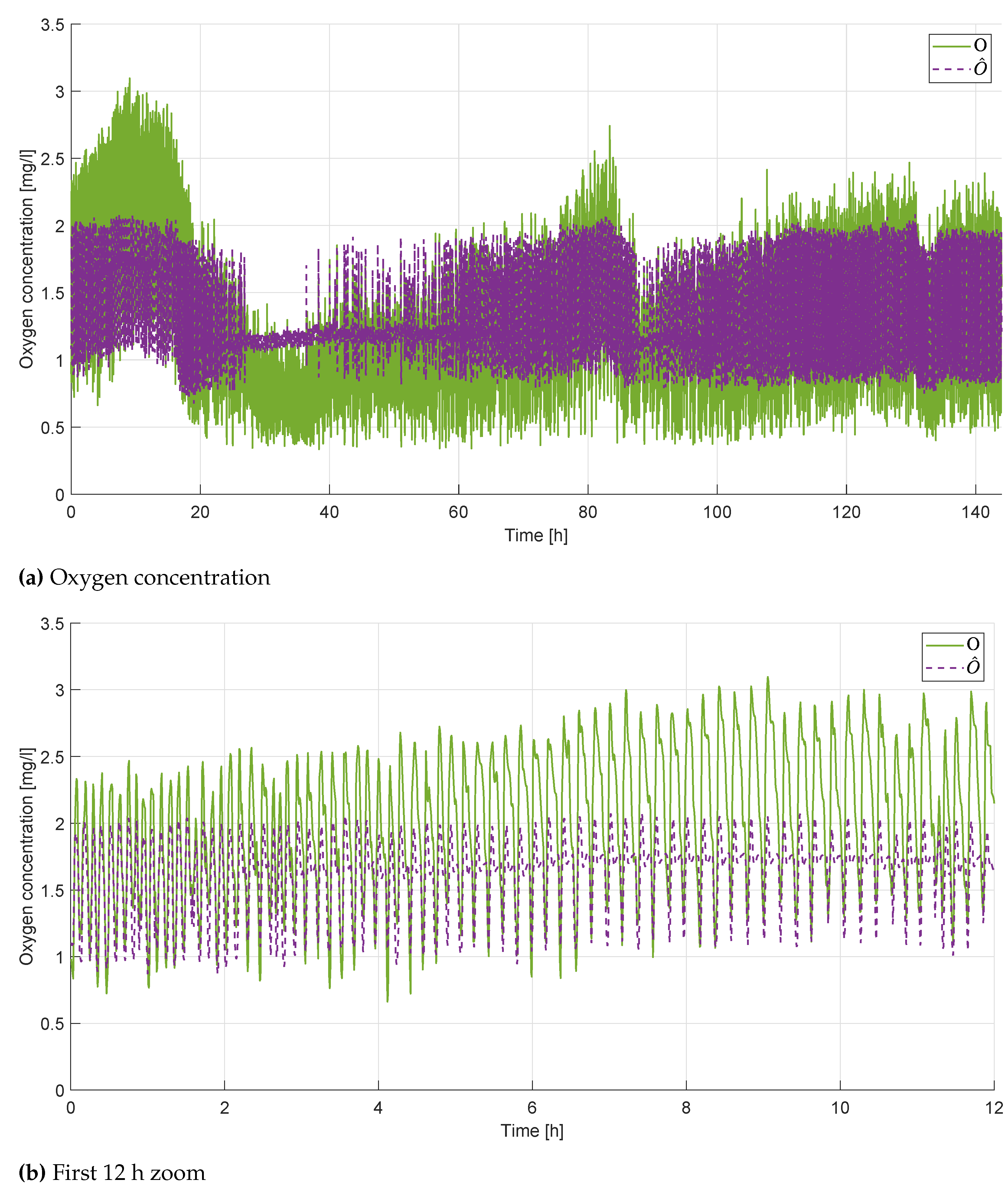
Figure 5.
Comparison of the results obtained with the LSTM and the ARX model during the first 6 h.
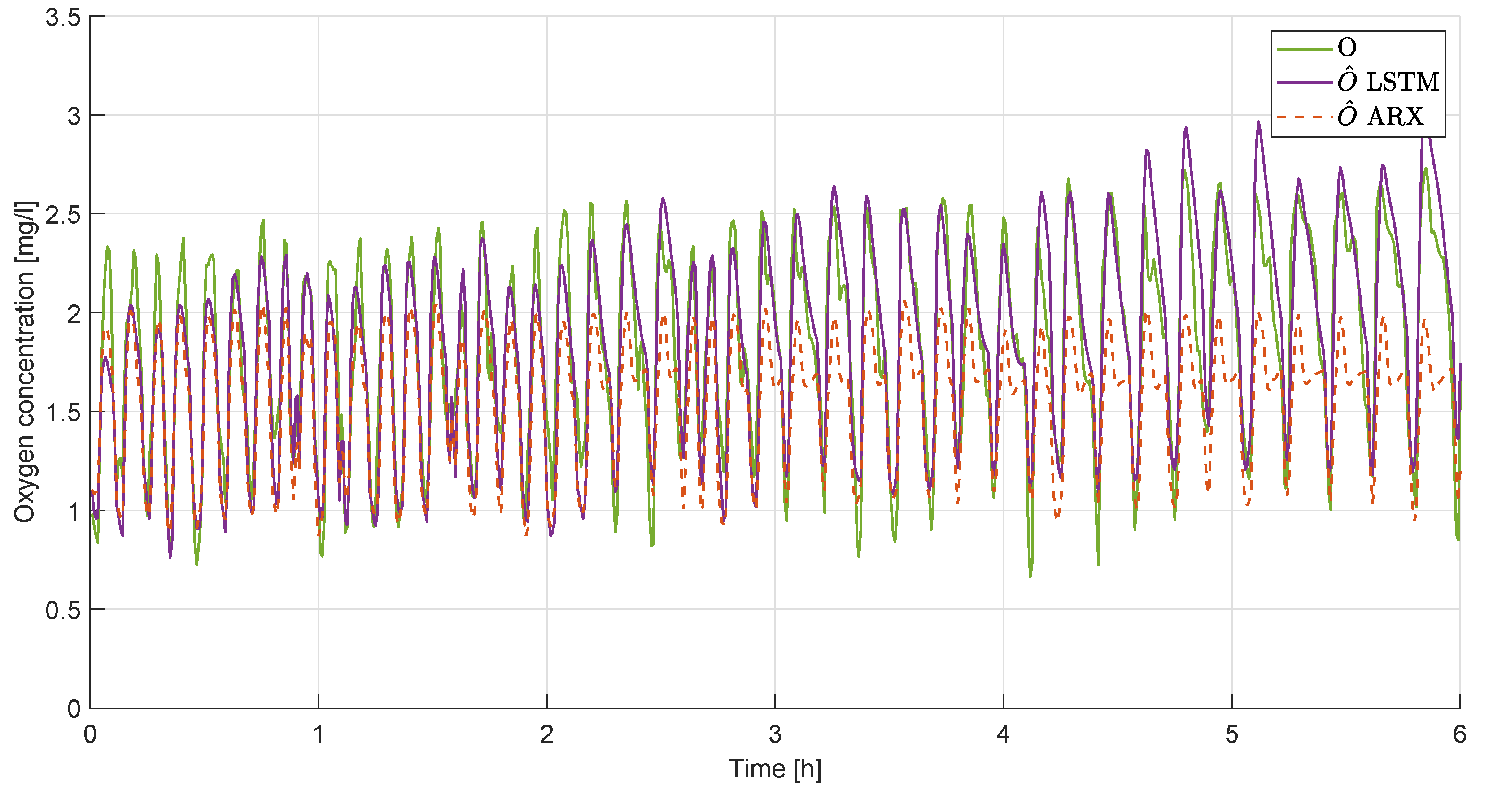

Table 1.
Compared ARX structures.
| signal | component | range | selected |
|---|---|---|---|
| order () | 10 - 17 | 12 | |
| order () | 2 - 12 | 6 | |
| delay () | 0 - 5 | 2 | |
| order () | 2 - 12 | 3 | |
| delay () | 0 - 10 | 5 | |
| order () | 3 - 9 | 7 | |
| delay () | 0 - 10 | 6 |
Table 2.
Datasets description.
| Dataset name | Start date | End date |
|---|---|---|
| Dataset 1 | 06/12/2021 | 11/12/2021 |
| Dataset 2 | 15/12/2021 | 20/12/2021 |
| Dataset 3 | 21/12/2021 | 26/12/2021 |
| Dataset 4 | 27/12/2021 | 01/01/2022 |
| Dataset 5 | 01/03/2022 | 06/03/2022 |
| Dataset 6 | 01/05/2022 | 06/05/2022 |
Table 3.
Model Comparison, results from Dataset1 simulation.
| Index | ARX | LSTM |
|---|---|---|
| 41.20% | 60.56% | |
| 0.833 | 0.921 | |
| 0.307 | 0.206 |
Disclaimer/Publisher’s Note: The statements, opinions and data contained in all publications are solely those of the individual author(s) and contributor(s) and not of MDPI and/or the editor(s). MDPI and/or the editor(s) disclaim responsibility for any injury to people or property resulting from any ideas, methods, instructions or products referred to in the content. |
© 2023 by the authors. Licensee MDPI, Basel, Switzerland. This article is an open access article distributed under the terms and conditions of the Creative Commons Attribution (CC BY) license (http://creativecommons.org/licenses/by/4.0/).
Copyright: This open access article is published under a Creative Commons CC BY 4.0 license, which permit the free download, distribution, and reuse, provided that the author and preprint are cited in any reuse.


