
Submitted:
07 February 2025
Posted:
07 February 2025
You are already at the latest version
Abstract
This paper investigates the application of recurrent neural networks, specifically Long Short-Term Memory (LSTM) models, for pressure forecasting in urban water supply systems. The objective of this study was to evaluate the effectiveness of LSTM models for pressure prediction tasks. To acquire real-time pressure data, an information system based on Internet of Things (IoT) technology using the MQTT protocol was proposed. The paper presents a data preprocessing algorithm for model training, as well as an analysis of the influence of various architectural parameters, such as the number of LSTM layers, the utilization of Dropout layers for regularization, and the number of neurons in Dense (fully connected) layers. The impact of seasonal factors, including month, day of the week, and time of day, on the pressure forecast quality was also investigated. The results obtained demonstrate that the optimal model consists of two LSTM layers, one Dropout layer, and one Dense layer. The incorporation of seasonal parameters improved prediction accuracy. The model training time increased significantly with the number of layers and neurons, but this did not always result in improved forecast accuracy. The results showed that the optimally tuned LSTM model can achieve high accuracy and outperform traditional methods such as the Holt-Winters model. This study confirms the effectiveness of using LSTM for forecasting in the water supply field and highlights the importance of pre-optimizing the model parameters to achieve the best forecasting results.
Keywords:
recurrent neural networks
; long short-term memory model
; hydraulic pressure
; water supply systems
; digital infrastructure
; Internet of Things
; pressure forecasting
; water supply reliability
1. Introduction
In the context of the development of the smart city concept, technical water supply systems are becoming a critical element in ensuring the sustainable transportation and distribution of vital resources. They play a key role in maintaining the stability of the urban environment, meeting the needs of the population, industry and utilities. However, with the development of social and technological infrastructure, water supply networks not only expand, covering ever larger territories, but also become more complex and branched. Such a structure increases the risk of ruptures and accidents due to equipment wear, uncontrolled loads or the influence of external factors, such as extreme weather conditions. Such emergency situations lead to serious environmental, economic and social consequences, including water leaks, environmental pollution and interruptions in the supply of urban consumers.
Traditional methods of responding to accidents in water supply systems involve detecting failures only after the actual failure, often based on calls received by the water utility dispatch service. This approach is not always effective, since the limited resources of operational repair teams or the remoteness of facilities lead to significant delays in troubleshooting, which increases the average time to restore water supply. However, with the development of the Internet of Things (IoT) technology, it has become possible to integrate smart sensors into monitoring systems, which allows collecting data on the state of the hydraulic network in real time. These data can be used to train machine learning models and subsequent digitization of the system state, ensuring early detection of potential accidents and increasing the efficiency of their elimination. In this regard, the objective of the study is to evaluate the effectiveness of using a recurrent neural network, namely its variety - the Long short-term memory (LSTM) model, in pressure forecasting problems. The scientific article examines the features of obtaining pressure data for training models, studies various architectures and their characteristics to improve the accuracy of pressure forecasting in water supply systems. The studies are carried out on the basis of the water supply system of the city of Gomel (Republic of Belarus), which has a significant length of pipeline networks. The scientific contribution of the article is expressed in the following positions:
1. The mechanism for obtaining data for training a hydraulic model based on the Internet of Things (IoT) technology using the MQTT protocol is considered. The process of collecting and preparing data is described in detail, including the difficulties and features that affect the quality of machine learning models.
2. The effectiveness of various neural network architectures used for interval pressure forecasting is studied. An analysis of the optimization of the internal network architecture is carried out, including an assessment of the influence of seasonal factors, the search for the optimal number of neurons in the LSTM model layers, the choice of the forecast horizon, the length of the historical sequence and the number of training epochs. All these aspects are considered to improve the accuracy and stability of the model when applied to water supply problems.
It is expected that the proposed approach to the selection and optimization of a machine learning model, in particular LSTM models, will allow establishing basic parameters for predicting pressure in water supply systems at the training stage. This approach will eliminate the need for long and resource-intensive processes of searching for optimal hyperparameters, which will significantly reduce the cost of computing resources for model training. This will provide the possibility of more rapid implementation of intelligent monitoring systems on the scale of large urban water supply networks and will increase their efficiency due to fast and accurate interval forecasting.
2. Related Works
Today, there are many methods for analyzing large volumes of data collected from sensors in real time, which allow for the timely detection of anomalies and potential threats. The introduction of machine learning algorithms makes it possible to predict time series of process parameters or create digital twins of technical systems, which becomes a powerful tool for modeling and testing various emergency scenarios. Predictive models act as a standard for assessing deviations in process parameters, which contributes to a deeper understanding of individual elements and the system as a whole. Within the framework of world experience, special attention in this context is paid to improving advanced methods that are used to prevent accidents, as well as assessing their contribution to improving the management and maintenance of water supply infrastructure. Despite the fact that the main attention in the article is given to water supply systems, artificial intelligence algorithms demonstrate high potential for application in related areas, such as gas supply, oil industry and heat supply. Analysis of examples presented in scientific publications confirms the effectiveness of these technologies in various industries, which opens up broad prospects for their adaptation and further development.
Of particular interest is the work [1], which examines in detail the use of machine learning methods in gas supply systems. The authors explore the potential of recurrent neural networks (RNN) and the K-nearest neighbors method for detecting gas leaks. The comparative analysis demonstrated that RNN models have significant advantages in tasks of this kind. This is due to their ability to adapt to new data, effectively learn on large volumes of information and take into account time dependencies, which is especially important for complex and dynamically changing conditions. The high accuracy of predictions achieved during the experiments emphasizes the potential of RNN as a tool for monitoring and managing infrastructure, where accurate detection and timely response are critical.
The study [2] presents the results of applying machine learning methods to model failure scenarios of pipelines with defects under pressure changes. The authors used approaches such as Artificial Neural Networks (ANN), Extreme Gradient Boosting (XGB) and CatBoost (CAT) categorical boosting. To train the models, data obtained from real pipeline inspections were used, as well as the results calculated by the finite element method for predicting ruptures. Comparative analysis showed that the CatBoost algorithm demonstrated the most accurate forecasts with minimal errors, which distinguishes it from other methods. This study emphasizes that the use of machine learning models such as CatBoost in combination with traditional analytical approaches significantly improves the efficiency of pipeline safety assessment. This becomes especially important in conditions of changing operating modes, where timely adjustment of process parameters is required to prevent accidents.
The study [3] presents the application of machine learning models to predict water pipe ruptures. The authors used gradient boosting algorithms implemented using the LightGBM (Light Gradient Boosting Machine) library developed by Microsoft. The main feature of the proposed approach is the comprehensive integration of various data, including engineering characteristics, geological conditions, climatic indicators and socio-economic factors. The results of the study demonstrate that taking into account social aspects along with technical parameters significantly affects the accuracy of emergency prediction. This method of risk assessment in water supply systems allows for a deeper analysis of the probability of failures, providing more effective management and accident prevention strategies. This emphasizes the potential of modern machine learning technologies for solving complex problems in the field of technical infrastructure.
Continuing with the topic of machine learning application in water supply systems, it is worth mentioning the study [4] published in the ISH Journal of Hydraulic Engineering. In this paper, the main focus is on the problem of water leakage monitoring using a reverse engineering approach. The authors proposed to solve classification and regression problems for leak detection by analyzing deviations in pressure or water flow using Artificial Neural Networks (ANN) and Support Vector Machines (SVM). The study was conducted in two scenarios: the first included the analysis of pressure data, the second - water flow data. To implement the tasks, the multilayered perceptron (MLP) and multi-layer classification and regression SVM models were developed. The results showed that ANN neural networks demonstrate higher accuracy in leak detection compared to SVM in both scenarios. It is also emphasized that optimizing the amount and quality of input data during the training process can significantly improve model performance, which remains an important direction for further research.
The review highlights a study conducted by [5], which is devoted to the use of coarse hydraulic models to control deviations in process parameters in water supply systems. The authors proposed an approach based on monitoring actual flow rates and pressures in pipelines, combined with machine learning methods. This method was tested on a reference water distribution network, where it demonstrated high efficiency in detecting anomalies. The results of the study emphasize that the integration of modern artificial intelligence and machine learning methods into the management of water supply systems can significantly improve the accuracy and efficiency of leak and emergency detection. This emphasizes the potential of such technologies to optimize the management of utility networks and improve their performance.
A study [6] published in the journal Applied Sciences presents a system for detecting and localizing leaks in water pipes using deep learning and Internet of Things (IoT) technology. The authors developed an approach based on intelligent sound leak detection and the use of convolutional neural networks (CNN). The experimental results demonstrate that the CNN model achieved an accuracy of over 95% after training, which highlights its high efficiency in the leak detection task. Additionally, it was shown that the use of this system can reduce excavation costs by 26%, significantly increasing the overall efficiency of pipeline infrastructure management.
The study [7] focuses on innovative approaches to predicting failures in water supply networks. The authors developed a classification model based on an Artificial Neural Network (ANN), using physical parameters of pipes (diameter, length, material, etc.) and operational indicators (flow rate, pressure, temperature, etc.) as input data. The effectiveness of the proposed method was analyzed taking into account two different data processing strategies. The first scenario examines the model’s performance under insufficient data, when the sample is too small for reliable training, and the second – under excess data, which can hinder analysis due to information overload. On real data from a Spanish water supply network, the ANN model demonstrated high accuracy, emphasizing the importance of balancing the volume and quality of data to ensure reliable forecasts.
In 2018, Onukwugha C. G., Osegi E. N. presented a study in which integrated system models combining machine learning and neural networks were used to monitor and forecast pressure in oil and gas pipelines [8]. The authors demonstrated that the combination of various technologies can significantly improve the accuracy and reliability of forecasts. This approach is an important example of the integration of classical hydraulic analysis methods with artificial intelligence algorithms, which can be adapted for water supply systems, opening up new opportunities for their management and prevention of emergency situations.
Continuing the discussion of innovative approaches to monitoring and forecasting in water supply systems, it is worth highlighting the study [9] devoted to the use of deep learning models to predict failures in water supply networks. In this work, the authors applied the Residual Neural Network (ResNet) algorithm and compared it with the classical Convolutional Neural Network (CNN). The results of the study showed that ResNet outperforms CNN in terms of training speed and forecasting accuracy. Particular attention in the study was paid to the role of physical parameters, such as the length and diameter of pipes, which turned out to be critical for assessing the risk of accidents. The authors concluded that the use of ResNet allows preventing more than half of the failures, focusing on servicing less than 10% of pipes, which significantly increases the efficiency of maintenance. Similar to the study by Onukwugha C. G., Osegi E. N., this work demonstrates how the integration of deep learning with advanced technologies can significantly improve the capabilities of monitoring and forecasting in water supply systems.
The review presents many modern approaches that demonstrate significant progress in the field of monitoring and prediction of failures in engineering systems, including water supply. The considered studies show that artificial intelligence and machine learning methods, such as artificial neural networks (ANN), support vector machines (SVM), gradient boosting (XGBoost, CatBoost, LightGBM), residual neural networks (ResNet) and convolutional neural networks (CNN), are successfully applied to solve problems of classification, regression and prediction in engineering networks. Among all the methods, a special place is occupied by recurrent neural networks (RNN) and their varieties, such as LSTM (Long Short-Term Memory), which, due to their ability to analyze sequential data and take into account temporal dependencies, are ideally suited for monitoring and prediction problems in water supply systems. This article focuses on the use of LSTM models as the main analysis method. This choice is due to their unique ability to process time dependencies and adapt to changing conditions, which allows achieving high efficiency and accuracy in predicting pressure in water supply systems.
3. Methods
The structure of the study consisted of several consecutive stages. At the first stage, a data collection and exchange scheme was developed, including connecting IoT devices, receiving information from pressure sensors, and transmitting it to a cloud storage system. This stage provided the basis for forming a statistical database and training models. At the second stage, data preparation was carried out: eliminating gaps, normalization, necessary transformations of time series, and dividing statistics into training and test data. At the next stage, the structure of the model class in Python was created, which included setting up the architecture, activation functions, optimizing hyperparameters, and training procedures. The last stage was devoted to training and testing the recurrent neural network (RNN) model using its LSTM variety. The effectiveness of the model was assessed based on metrics such as MAE, SMAPE, MAE, and RMSE.
3.1. Organization of Data Collection for Monitoring Pressure in a Water Supply System
An information system has been developed for operational monitoring and archiving of pressure parameters of pumping stations in the water supply system of Gomel (Republic of Belarus). Within the framework of this system, adhering to the concept of the Internet of Things (IoT), a network of interconnected smart devices was deployed that automatically collect, exchange and process data [10]. Figure 1 shows the diagram used, demonstrating the connection of pressure sensors to data collection and transmission devices that polled these sensors and sent the received information in raw form to the computing server [11]. To ensure the reliability of receiving and transmitting information, a specialized Mosquitto broker (MQTT broker) was installed on the server, acting as a central node. It ensured the coordination of data transmission between data publishers (pressure sensors) and subscribers [12] (personal computers, telephones). The developed architecture facilitated prompt response to changes in system parameters and the formation of statistical data for subsequent training of the long short-term memory model.
In the context of this study, the data sources were PD100 piezoelectric pressure transducers of the Russian Oven trademark. This choice was due to the high accuracy of the device, which was critical for the formation of a reliable pressure database at the inlet of pumping stations. The pressure sensors were connected directly to the pressure gauges (Figure 2 b) according to a specific layout on the city map in accordance with the identified water consumption clusters [13]. This made it possible to quickly organize the installation of equipment in the most significant water supply units. It is worth noting that in the absence of pressure gauges, connecting the sensors requires more complex operations that require preparatory welding. RTU-8xx modems from Teleofis (Figure 2, a), configured for 5-minute measurements and sending messages to the cloud server, served as data collection and transmission devices.
3.2. Features of Data Preparation for Model Training
To train the recurrent neural network (RNN) model, it is important to properly prepare the data. The pressure data in the water supply network was collected using piezoelectric sensors equipped with a telemetry output standardized for the range of 4–20 mA. Raw values in this range were received by the server, which required preliminary transformation before being used in the forecasting model. The current values coming to the cloud server were scaled using linear interpolation to the pressure according to the formula:
where – actual pressure value;, – minimum and maximum pressure sensor value; – actual current value;, – minimum (4 mA) and maximum (20 mA) current value.
On the server side, storage of both raw and transformed pressure data is organized. Raw data included time stamps corresponding to the moment of data collection, as well as current values obtained from the sensors. Transformed data are pressure values calculated using formula (1) based on the received current. As a result, the database took the form «epoch – pressure», where the first parameter is the time stamp (Unix time), and the second is the transformed pressure value. This approach allowed storing data in its original form for further processing and analysis, as well as using ready-made transformed values for training models. An example of such data is presented in Table 1.
The initial statistics then underwent pre-processing, which included removing outliers, filling in missing values, and normalizing features. The latter is recommended to improve the learning process and solution convergence [13]. In this case, min-max normalization is used to bring features to the range from 0 to 1:
where , – normalized and original feature;, – the largest and smallest element of a feature.
Thus, the initial data took the form of a matrix of size T × N. Here T is the number of time points (or measurements) of the time series, and N is the number of features corresponding to each moment in time. In the example of Table 1, the initial data set was determined by a single pressure parameter p at time t. In this case, N is equal to 1 and the matrix form of recording took the following form:
In the study, the Keras library in Python [14] was used to train the long short-term memory (LSTM) model. One of the features of training the LSTM model is the need to represent the input data as a multidimensional tensor. In particular, recurrent neural networks expect the data to be in the form of a three-dimensional tensor, where the first axis represents the number of observations (samples) in the data, the second axis corresponds to the length of the time interval or window, which determines the depth of history taken into account by the model when predicting pressure, and the third axis reflects the number of features that are used to predict future values. The transition of the original matrix A to a multidimensional form to form the input tensor in the LSTM model included the following steps:
1. The depth of the observation history M was determined, which is one of the parameters of further research, which was selected depending on the accuracy of pressure forecasting (Figure 3). This parameter determines the size of the time window through which the model can «see» changes in the feature over a certain period of time. The depth of the history M allows the model to take into account the influence of past values on the forecast of future values of the output pressure sequence.
2. The optimal forecast horizon of length K was determined (Figure 3). The minimum forecast error at each step of the interval window and the average error of the resulting sequence served as the criterion.
3. The study used various architectures to extract additional factors from the original timestamp (epoch). In particular, such features as minute, hour of day, month index, day of the week type (working or weekend) were additionally extracted. This expanded the original matrix, increasing the number of input features. For each of these features N, a set of time windows of length M was formed, extracted from the original matrix A. The number of such windows was T – M. Further, each of these windows became a sample of dimension M×N, that is, it contained M observations for each of the N features. In total, T – (M + K) data sets were obtained for training the model (since for each sample it is necessary to have a corresponding output sequence of length K), which determines the number of samples in the three-dimensional tensor.
4. To increase the volume of training data, the rolling window approach was used [15,16]. This method involved forming a set of overlapping sequences, which was achieved by shifting the time series by a given interval (Figure 4). This significantly increased the sample size for training the model. For the initial training data with the number of observations T, the shift step S was specified. Then, for each i-th position of the window with the shift step S = 1, the data samples are in the range , where is the possible number of observations. The training matrix A will contain elements , where i = 1, 2, ..., , ; j = 1, 2, ..., M + K.
5. Matrix A was divided into two parts, defining the input data X with elements , where i = 1, 2, ... , ; j = 1, 2, ..., M and the output (target) data Y with elements , where I = 1, 2, ..., ; j = M + 1, M + 2, ..., M + K. The resulting matrix is reduced to a tensor form, taking into account the number of features of the model:
where – the input layer matrix of the neural network has dimension М×N, where each column represents the i-th subsequence of length M for each of the N features in the time series. Similarly, the output layer of the matrix has dimension , where each column contains information about K prediction values for each of the P parameters. In this study, one pressure parameter was predicted.
3.3. Features of Assessing the Effectiveness of the Learning Process
At the training stage, the search for optimal model parameters was carried out, such as the history length (M) and prediction depth (K), the number of neurons in the layers of the long short-term memory model (NLSTM). The main goal was to find the LSTM architecture that would provide the maximum accuracy of hydraulic pressure forecasting [17,18]. To assess the quality of the predictive model, the cross-validation method was used, namely block cross-validation [19]. This method is based on dividing the time series into non-overlapping blocks using a sliding window with a given step. Instead of repeatedly training the model on different data blocks, the model was trained once using the initial architecture settings, which were then changed to find the best configuration. After that, the effectiveness of the model was assessed on the test set. The procedure for assessing the quality of learning algorithms used in these studies included:
1. Splitting the data into training and test samples: a time series of length T+L (Figure 5) was split into a training sample of length T and a test sample of length L in a ratio of 70% to 30%.
2. Dataset generation: In the forecasting process, a sliding window method with a given step was used to obtain new test data [15]. For each time step t (starting from the first element of the test sample to the end of the time series L), a data block of length M (data history) was used as input and the next K elements were used as the target variable. This formed a dataset of size (T – M – K + 1) x (M + K), where each row contains one set of input and output data (Figure 5).
3. Prediction for a given interval: at each step t, the model made a prediction for a given interval ahead K. The results of the predictions were saved for further analysis.
4. Model quality assessment: The obtained predictions were compared with real observations. A distinctive feature was the assessment of both the average error at each step of the block displacement t over the entire depth of the forecast K, and the calculation of the average error of all predictions. In the studies conducted, classical metrics were used to assess the quality of the pressure forecasting model: MAPE (mean absolute percentage error), MAE (mean absolute deviation) and RMSE (root mean square error). Despite the widespread use of MAPE, this metric does not effectively cope with zero values, which is typical for scenarios related to an emergency pressure drop or on/off modes of pumping stations (Figure 6). In such cases, MAPE gave a distorted estimate due to the mathematical uncertainty that occurs when dividing by zero.
To solve this problem, the SMAPE (symmetric mean percentage error) metric was used as an alternative, which works more stably in such conditions, since it excludes infinite values and gives a more correct assessment of the accuracy of the model at zero pressure values [20]:
where – actual value at the i-th moment in time; – predicted value at the i-th moment of time; – number of observations.
3.4. Finding the Optimal Architecture and Hyperparameters of the LSTM Model
The goal of the study was to find an LSTM model architecture that would ensure high forecasting accuracy and efficient use of computational and information resources during training. To achieve these goals, various combinations of hyperparameters were used before training. The search for the optimal model structure included the following stages:
1. Assessing the impact of adding additional layers to the LSTM model - we studied how an increase in the number of layers affects the accuracy of the model and its ability to generalize.
2. Assessing the impact of parameters that determine seasonality - we analyzed the effectiveness of adding seasonal parameters.
3. Assessing the impact of the number of neurons in model layers - we studied the dependence of the model accuracy on the number of neurons in hidden layers.
4. Assessing the impact of the amount of historical data and forecasting range - we analyzed the effect of increasing the volume of training data and further forecasting steps on the accuracy of modeling.
Figure 7 shows a general view of the structure of the long short-term memory model and the relationships between the layers, the network, and the optimization function of the model under study.
The model was tested on statistical data presented by 5-minute discreteness of the input pressure of the booster pumping station on Artilleriyskaya Street in Gomel for the period from 17.02.2023 to 16.03.2023. The size of the original statistics: [13398, 2], where the first parameter determines the generated number of observations; the second - two features: epoch, pressure.
4. Results and Discussion
4.1. Optimization of the Internal Architecture of the Neural Network
The study tested the impact of additional layers on the model performance. For this purpose, the basic architecture was used, within which the following parameters were fixed: the number of neurons in the LSTM layers and the fully connected layer was 50; the number of historical observations fed to the model input was 12; the length of the output sequence, the number of predicted values was 12; and the number of input parameters was 1 (pressure with 5-minute discretization). These parameters were selected for the initial setup of the model, after which various configuration options were tried to assess their impact on the forecasting accuracy. In total, 7 different architectures with different combinations of the number of LSTM, Dropout, and Dense layers were considered [21,22]. The results of the model performance evaluation are presented in Figure 8.
The study revealed the following:
1. Increasing the number of LSTM layers to 2-3 improves the forecast quality and reduces the MAPE, SMAPE, MAE, and RMSE metrics compared to a single-layer LSTM architecture.
2. Adding a regularization layer (Dropout) improves model performance. Models with one or two Dropout layers show a lower forecast error compared to models without adding Dropout layers.
3. Adding additional fully connected layers (Dense) does not always improve model performance. In this study, models with one Dense layer show better results compared to models with two Dense layers.
4. Model training time increases with the number of layers and model dimension. Models with more layers and parameters require more time to train. The model with three LSTM layers, Dropout and Dense without changing the forecast quality on 20 epochs required twice as much time for training compared to the model consisting of two LSTM layers and one Dropout and Dense. Based on the analysis, we can conclude that the optimal model has 2 LSTM layers, 1 Dropout layer and 1 Dense layer. The error of the given model on the test data was MAPE = 4.79%.
4.2. Evaluation of the Impact of Seasonal Components on the Efficiency of the Model
The study of the influence of seasonality parameters on the quality of the LSTM model was carried out by adding various combinations of time factors to the input layer of the recurrent neural network. The seasonality parameters were month, time (hours and minutes), and day of the week type. The data for training the model was collected for two months - September and October 2022. The short time interval did not allow us to fully assess the variation of the month during the year and its impact on the forecasting results. In practice, this can be eliminated by continuous retraining of the model, when, as new data is received, the model is constantly updated and adapted to new data. The «day type» factor had minimal variability and took only two values: a working day or a day off. Holidays and pre-holiday days were not included in the training set. Nevertheless, the results shown in Figure 9 show that the inclusion of various combinations of seasonality parameters affects both the quality of forecasts and the training time of the model.
The analysis results show that in the case when the input statistics did not take into account seasonal factors, the model showed the following results: MAPE – 4.77%, SMAPE – 4.71%, MAE – 8.0 kPa, RMSE – 10.3 kPa. Adding day type as the only seasonal parameter led to a slight increase in MAPE to 4.81%, while SMAPE remained at 4.71%. Adding minute as the only seasonal parameter increased the MAPE and SMAPE values to 4.78%, and MAE – to 8.1 kPa. Using minute and day type together increased the training time, but did not lead to a significant improvement in the metrics. Taking into account the hour of day in the model increased MAPE and SMAPE to 4.9%, and also increased MAE and RMSE. The best result was achieved when using all four parameters: month, hour, minute, and day type. This resulted in a MAPE of 4.37%, SMAPE of 4.34%, MAE of 7.4 kPa and RMSE of 9.4 kPa.
There are several key findings from examining the impact of seasonal components on model performance:
1. Impact of Seasonality: Including seasonality parameters such as month, hour, minute, and day type in a model improves its predictive ability. Overall, models that include these parameters perform better on all evaluation metrics than models without seasonality parameters. This may be because these parameters help the model capture structure in the data that would be invisible without them.
2. Training Time: Including more seasonality parameters increases the training time for the model, which is due to the larger number of parameters required to process and train the model. However, it is important to note that despite the increased training time, models with more parameters generally perform better predictively.
3. Optimal Combination: The lowest MAPE, SMAPE, MAE, and RMSE scores are demonstrated by the model that includes all four seasonality parameters: month, hour, minute, and day type. This indicates that using all of these parameters together results in improved forecast accuracy.
It is worth noting that training the model with seasonal components does not change the procedure for obtaining information from primary converters and does not increase the volume of the database stored on the server. Information about the month, hour, minute and day type is extracted through the Unix timestamp transformation. This allows seasonality to be taken into account in the data without additional accumulation of information.
4.3. Finding the Optimal Number of Neurons in LSTM Model Layers
The choice of the model configuration is based on the grid search method, which is used to determine the optimal number of neurons in the LSTM and Dense layers of the neural network [23,24,25]. In accordance with this method of model training, an algorithm for cyclic enumeration of all possible combinations of hyperparameters is implemented. To enumerate various combinations in each layer, a list of neurons for each of the three layers of the model (two LSTM layers and one Dense layer) with values of 50, 150 and 250 was formed. In the conducted study, 21 models were trained with a total time cost of 110019 sec. (30.6 h). During the study, it was noted that an increase in the number of neurons in the first and second LSTM layers leads to a significant increase in the model training time. However, no corresponding improvement in the quality of model forecasts is observed. This confirms the assumption that the complexity of the model does not always correlate with its performance. In connection with the above observations, it was decided to stop the cyclic enumeration of parameters after reaching the specified configuration. Figure 10 shows the distribution diagram of the MAPE forecast error indicator when changing neurons in the LSTM layers and one Dense model.
According to the obtained results, it follows:
1. The error rates vary in a small range. This indicates that changing the number of neurons in each layer does not lead to a significant improvement or deterioration in the accuracy of the forecast. The lowest error rates are observed in experiments #3 and #21 (L1=50, L2=50, D=250 and L1=250, L2=50, D=250, respectively). This may indicate that increasing the number of neurons in the Dense layer with a relatively small number of neurons in the LSTM layers, taking into account the resource costs for training, may be more effective for the task under study.
2. The training time of the models varies significantly and, as a rule, increases with an increase in the number of neurons. The fastest learning occurs with the smallest number of neurons (L1=50, L2=50, D=50), the slowest – with the largest (L1=150, L2=250, D=150 and L1=150, L2=250, D=250).
3. In this problem, increasing the number of neurons in the layers does not always lead to an improvement in the forecast accuracy. At the same time, the training time increases significantly, which can be critical with limited computing resources. Based on these results, we can conclude that the optimal configuration is a model with 50 neurons in the LSTM layers and 250 neurons in the Dense layer as the most optimal in terms of the ratio of forecast accuracy and training time. In some cases, the growth of neurons in the first LSTM layer leads to an improvement in the quality of the model. With limited resources, the LSTM and Dense layers can be reduced to 50 neurons, which leads to the minimum training time of the considered configurations.
4.4. Selecting the Optimal Length of the Input and Output Data Sequence
The length of the history sequence refers to the number of previous time steps that the model uses for training and subsequently for predicting the target variable. If the history depth is too small, the model may not have enough information to identify important time patterns, otherwise training the model may become complex and expensive in terms of computational time. The conducted experiment to find the optimal ratio of the history length and the forecast horizon took 95257 seconds over 20 epochs of model training. In this case, various combinations of input and output data were tried with an assessment of the model quality metrics. In the conducted study, 20 different sets of parameters with history [12,24,36,48,60] and forecast [12,24,36,48] depths were considered. The figure shows the results of the analysis of the influence of the history depth and the forecast horizon length on the change in the MAPE metric over 20 epochs of model training. In Figure 11 shows the results of the analysis of the influence of the depth of history and the length of the forecasting horizon on the change in the MAPE metric for 20 epochs of model training.
As a result of the experiment, the following conclusion can be made:
1. With an increase in the length of the input data (history depth), the model training time increases significantly, which is associated with an increase in the dimension of the data tensor, as a result of which more computing power and time are required to train the model.
2. With an increase in the length of the forecasting horizon, no stable growth or decrease in the model quality metrics is observed. This may indicate that the dependence between the forecasting horizon and the quality of the model may be non-linear or may change significantly depending on other factors.
3. Models with fewer input and output data usually show better results in terms of quality and performance metrics.
4. In certain cases, it was observed that an increase in the length of the output data with a constant length of the input data leads to a deterioration in the quality of the model.
Of particular interest is the change in the loss function during the model training process. To do this, the number of epochs was increased from 20 to 50 and the behavior of the mean square error was assessed for cases with 12, 24 and 60 time steps entering the LSTM model (Figure 12).
Analyzing the results of the experiment, we can conclude that with increasing history depth, a more stable behavior of the mean square error is observed without significant outliers. This indicates better convergence of the model, that is, optimal adjustment of weight coefficients during the training process when receiving a larger amount of input data. A stable decrease in the loss function indicates that the model is more effective in learning on data with 60 time steps compared to 12, but the training time for 200 epochs increased by 50%, the metric on the MAPE test data was 4.36%.
4.5. LSTM Models Compared with Holt-Winters Model
An important step in the study is to demonstrate the advantages of deep learning models. For this purpose, the LSTM model used is compared with the classical simpler Holt-Winters exponential smoothing model [26]. Additive seasonality with a period of 288, which characterizes the daily dynamics with 5-minute pressure data, is used as the initial parameters of the exponential smoothing model. Comparison of the quality metrics of the models was carried out on test data, which included statistics including an emergency pressure drop at the inlet of the booster pumping station (Figure 13). The LSTM model demonstrates a lower forecasting error compared to the Holt-Winters model. The MAPE value for the LSTM model is 4.36%, while the Holt-Winters model has an average absolute percentage error of 6.07%. The MAE metric was 7.35 and 9.86 kPA for the first and second models, respectively. Based on these results, it can be concluded that the LSTM model has a higher quality and provides more accurate data prediction.
It is worth paying special attention to the behavior of the model during an emergency pressure drop. In Figure 13, the LSTM model is built with a forecast for 12 steps (1 hour into the future), while the length of the historical data fed to the model was 60 values (5 hours of history). It is interesting to note that the recurrent neural network model is able to notice and respond to the falling pressure dynamics, even though in the considered example the training sample had only one emergency scenario. This indicates high sensitivity and the ability of the model to detect changes in time series, even with limited data at the time of a sudden pressure drop, which does not allow the implementation of the Holt-Winters model.
Conclusions
In the course of this study, an information system for obtaining data on hydraulic pressure in a water supply system was developed. These data were subsequently used to train a long short-term memory (LSTM) model designed to predict pressure in a water supply system and use these forecasts to create preventive methods for responding to accidents. An important stage of the work was to study the influence of the neural network architecture on its performance. It was found that increasing the number of LSTM layers (up to 2-3) and using regularization layers (Dropout) contributes to improving the forecast accuracy, while adding additional fully connected layers does not have a significant effect. The optimal configuration of the model includes two LSTM layers, one Dropout layer and one Dense layer, which provided minimal values of error metrics such as MAPE (4.79%). In addition, a study was conducted on the influence of seasonal factors on forecasting accuracy. It was found that adding parameters such as month, hour, minute and day type leads to an improvement in the quality of the model and a reduction in forecast errors (MAPE decreased to 4.37%).
The influence of the number of neurons in the LSTM and Dense layers on the model performance was also assessed using the grid search method. Based on the obtained data, the optimal model configuration with 50 neurons in the LSTM layers and 250 neurons in the Dense layer was selected, which provided the best ratio of forecast accuracy and training time. In parallel, the influence of the length of the input and output sequences on the quality of the model was investigated. Increasing the length of the input data (history depth) improved the convergence of the model, but also increased the training time. Models with less data demonstrated faster results with comparable forecast accuracy. This confirms that the optimal choice of history depth and forecast length depends on the computing resources and the tasks at hand.
In the final part of the work, the proposed LSTM model was compared with the classical Holt-Winters exponential smoothing model. The results showed that LSTM significantly outperforms the Holt-Winters model both in forecast accuracy (MAPE 4.36 versus 6.07%) and in sensitivity to emergency situations, such as a sharp drop in pressure. Thus, the experiments showed that the use of LSTM models for forecasting pressure in water supply systems significantly improves the accuracy of forecasts, especially when including seasonal factors and optimizing the model architecture. The study is not exhaustive, and other combinations of hyperparameters may be more effective for the task of forecasting water supply network pressure.
Author Contributions
Conceptualisation, AAK, NVH, RVK; methodology, SNS, EAE; software, AEB; validation, SNS, EAE; formal analysis, NVM; investigation, AYD; resources, AYD; data curation, AYD; writing-original draft preparation, AAK, RVK; writing-review and editing, NVM; visualisation, AEB. All authors have read and agreed to the published version of the manuscript.
Funding
This research received no external funding.
Institutional Review Board Statement
Not applicable.
Informed Consent Statement
Not applicable.
Data Availability Statement
The data presented in this study are available from the corresponding authors upon reasonable request.
Conflicts of Interest
The authors declare no conflicts of interest.
References
- Ezechi, C.G.; Okoroafor, E.R. Integration of Artificial Intelligence with Economical Analysis on the Development of Natural Gas in Nigeria; Focusing on Mitigating Gas Pipeline Leakages. SPE Nigeria Annual International Conference and Exhibition. SPE, 2023.
- Liu, W.; Chen, Z.; Hu, Y. Failure Pressure Prediction of Defective Pipeline Using Finite Element Method and Machine Learning Models. SPE Annual Technical Conference and Exhibition. OnePetro, 2022.
- Fan, X. Machine learning based water pipe failure prediction: The effects of engineering, geology, climate and socio-economic factors. Reliability Engineering & System Safety 2022, 219, 108185. [Google Scholar]
- Sourabh, N.; Timbadiya, P.V.; Patel, P.L. Leak detection in water distribution network using machine learning techniques. ISH Journal of Hydraulic Engineering, 2023; 1–19. [Google Scholar]
- Momeni, A.; Piratla, K.R. Prediction of Water Pipeline Condition Parameters Using Artificial Neural Networks. Pipelines 2022, 2022, 21–29. [Google Scholar]
- Tsai, Y.L. Using convolutional neural networks in the development of a water pipe leakage and location identification system. Applied Sciences, 2022; 12, 8034. [Google Scholar]
- Robles-Velasco, A. Artificial neural networks to forecast failures in water supply pipes. Sustainability, 2021, 13(15), 8226. 13(15).
- Onukwugha, C.G.; Osegi, E.N. An Integrative Systems Model for Oil and Gas Pipeline Data Prediction and Monitoring Using a Machine Intelligence and Sequence Learning Neural Technique, 2018.
- Liu, W.; Xie, Z.; Song, Z. Predicting Water Pipe Failures Using Deep Learning Algorithms. Journal of Infrastructure Systems, 0402. [Google Scholar]
- Zyrianoff, I. Scalability of an Internet of Things platform for smart water management for agriculture. 2018 23rd conference of open innova-tions association (FRUCT). IEEE.
- Thangavel, D. Performance evaluation of MQTT and CoAP via a common middleware. 2014 IEEE ninth international conference on intelligent sensors, sensor networks and information processing (ISSNIP). IEEE.
- Naik, N. Choice of effective messaging protocols for IoT systems: MQTT, CoAP, AMQP and HTTP. 2017 IEEE international systems engineering symposium (ISSE). IEEE.
- Kapanski, A.A.; Klyuev, R.V.; Boltrushevich, A.E.; Sorokova, S.N.; Efremenkov, E.A.; Demin, A.Y.; Martyushev, N.V. Geospatial Clustering in Smart City Resource Management: An Initial Step in the Optimisation of Complex Technical Supply Systems. Smart Cities 2025, 8, 14. [Google Scholar] [CrossRef]
- Buda, M. , Maki, A.; Mazurowski, M.A. A systematic study of the class imbalance problem in convolutional neural networks. Neural Networks, 2018, 106, 249–259. [Google Scholar] [CrossRef] [PubMed]
- Chollet, F. Deep Learning with Python. Manning. 2021; ISBN 9781617296864. [Google Scholar]
- Shen, L.; Wei, Z.; Wang, Y. Determining the Rolling Window Size of Deep Neural Network Based Models on Time Series Forecasting. Journal of Physics: Conference Series, 2021, 2078, 012011. [Google Scholar] [CrossRef]
- Hewamalage, H.; Bergmeir, C.; Bandara, K. Recurrent neural networks for time series forecasting: Current status and future directions. International Journal of Forecasting. [CrossRef]
- Hochreiter, S. Long Short-term Memory. Neural Computation, 1735. [Google Scholar] [CrossRef]
- Bengio, Y.; Simard, P.; Frasconi, P. Learning long-term dependencies with gradient descent is difficult. IEEE Transactions on Neural Networks. [CrossRef]
- Bergmeir, C.; Hyndman, R.J.; Koo, B. A note on the validity of cross-validation for evaluating autoregressive time series prediction. Computational Statistics & Data Analysis, 2018, 120, 70–83. [Google Scholar]
- Kreinovich, V.; Nguyen, H.T.; Ouncharoen, R. A: to estimate forecasting quality, 2014.
- Srivastava, N. Dropout: A simple way to prevent neural networks from overfitting. The journal of machine learning research, 1929. [Google Scholar]
- LeCun, Y.; Bengio, Y.; Hinton, G. Deep learning. Nature, 2015; 521, 436–444. [Google Scholar]
- Bergstra, J.; Bengio, Y. Random search for hyper-parameter optimization. Journal of machine learning research, 2012; 13. [Google Scholar]
- Karl, F.; Pielok, T.; Moosbauer, J.; Pfisterer, F.; Coors, S.; Binder, M.; Bischl, B. Multi-Objective Hyperparameter Optimization--An Overview, 2022. arXiv:2206.07438.
- Hutter, F.; Kotthoff, L.; Vanschoren, J. Automated machine learning: Methods, systems, challenges. Springer Nature.
- Taylor, J.W. Short-term electricity demand forecasting using double seasonal exponential smoothing. Journal of the Operational Research Society.
Figure 1.
Architecture of data exchange during experiments.
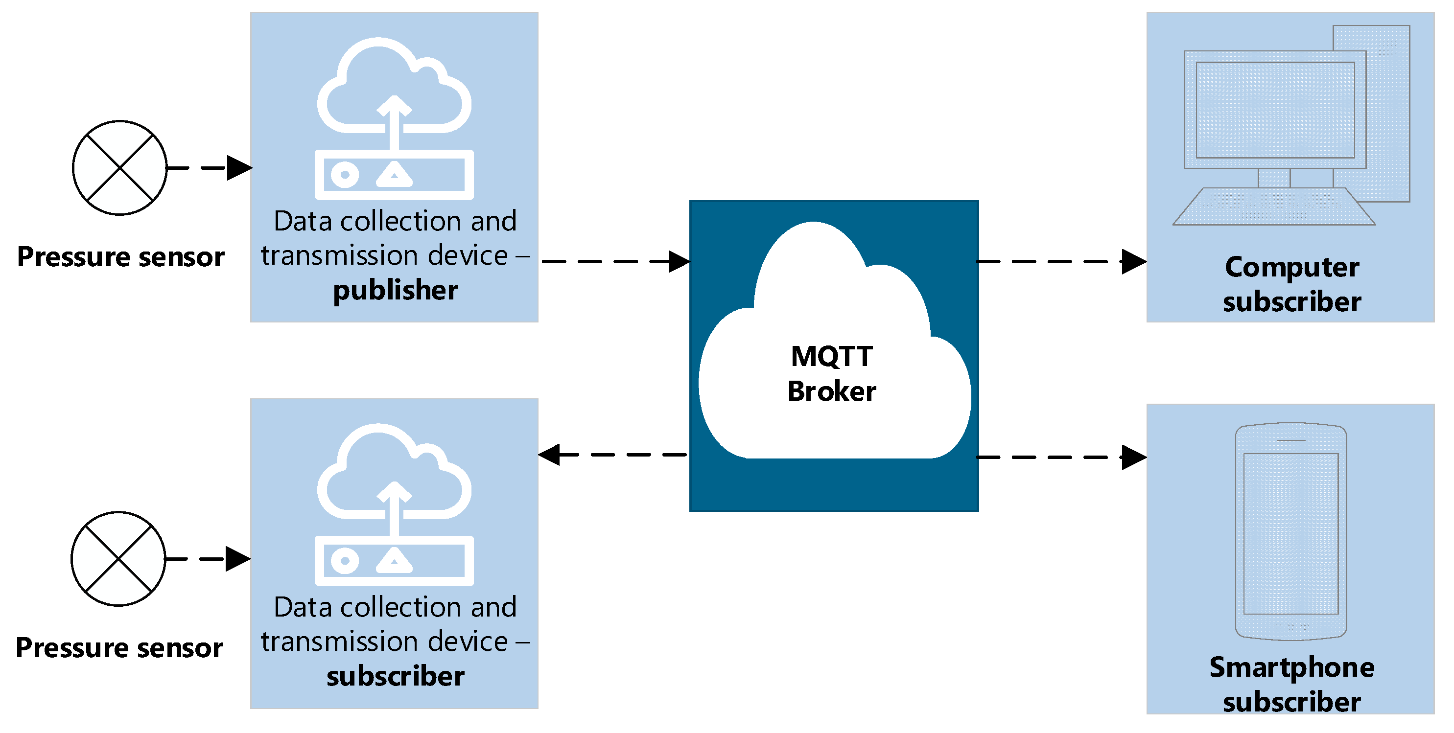
Figure 2.
The process of connecting the pressure transducer at the pumping station to the data collection and transmission device.
Figure 2.
The process of connecting the pressure transducer at the pumping station to the data collection and transmission device.

Figure 3.
A fragment of a sample of input and output sequence of a given length.
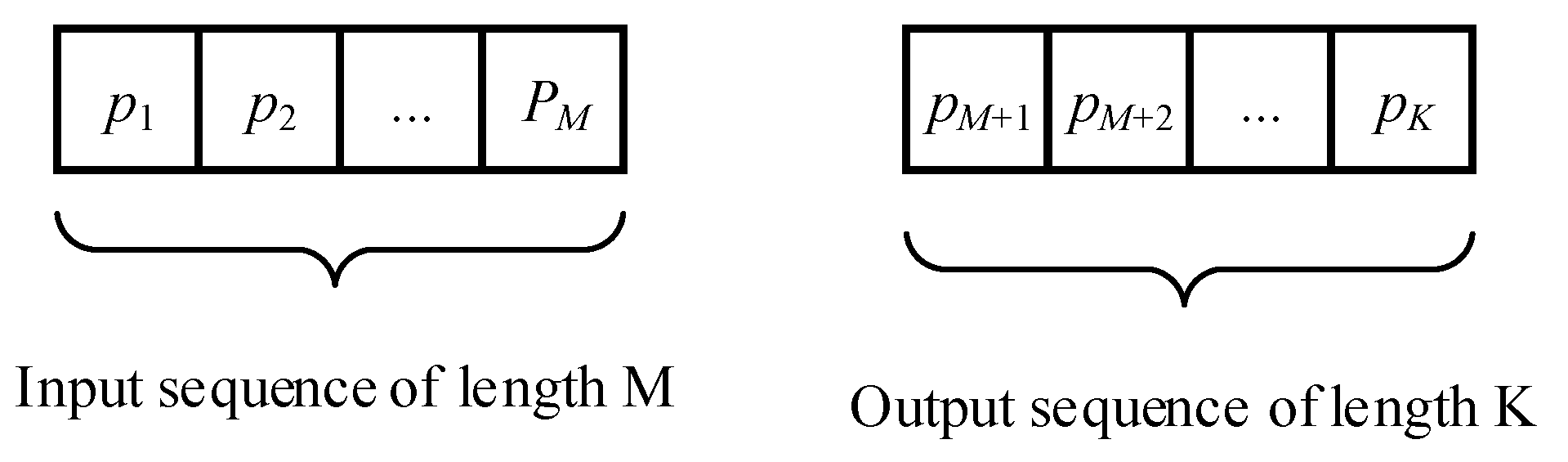
Figure 4.
To explain the use of the sliding window method to increase the statistics set.
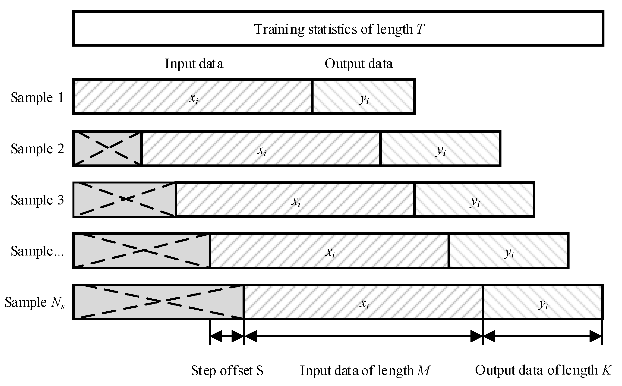
Figure 5.
Interpretation of the cross-validation method used.
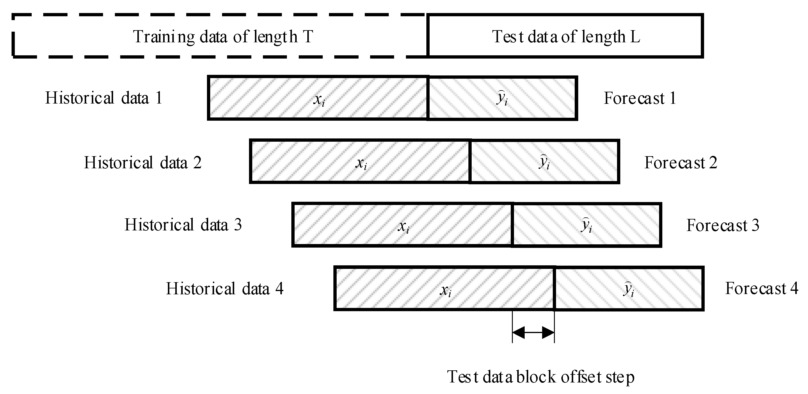
Figure 6.
Switching on and off mode of the pumping station in the village of Bobovichi, Gomel district.
Figure 6.
Switching on and off mode of the pumping station in the village of Bobovichi, Gomel district.

Figure 7.
Towards an explanation of the choice of the LSTM neural network model architecture.
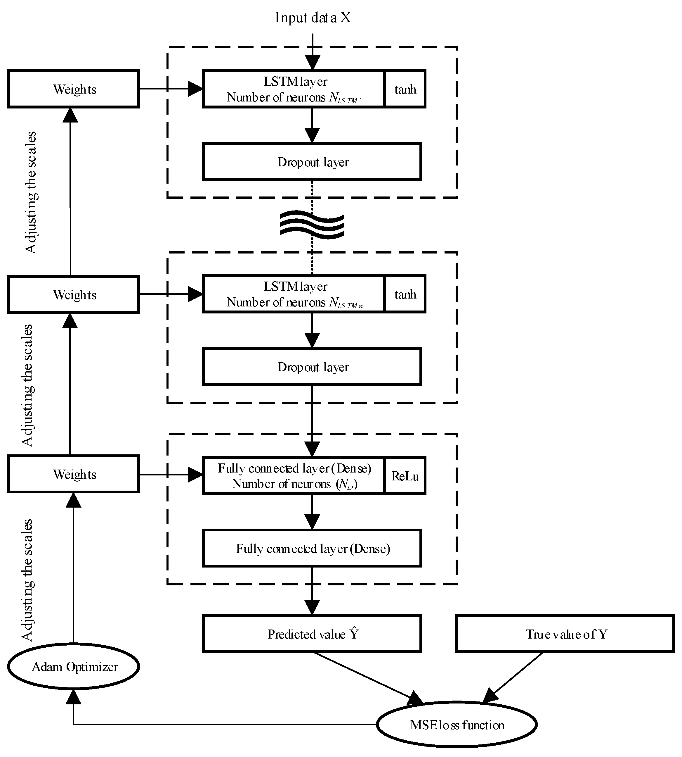
Figure 8.
The Impact of Neural Network Architecture on Model Performance.
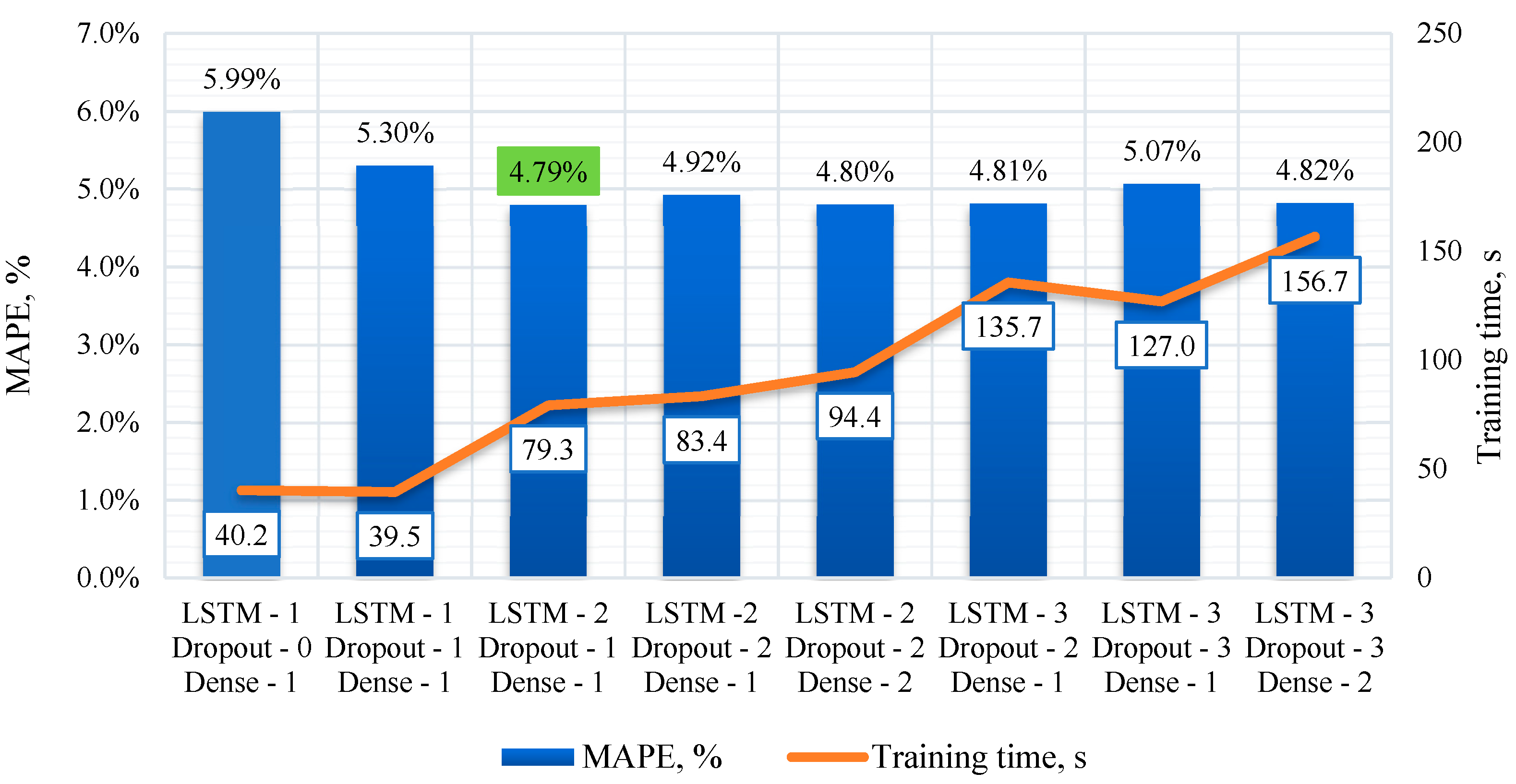
Figure 9.
The influence of seasonal components on the quality of the pressure forecasting model.
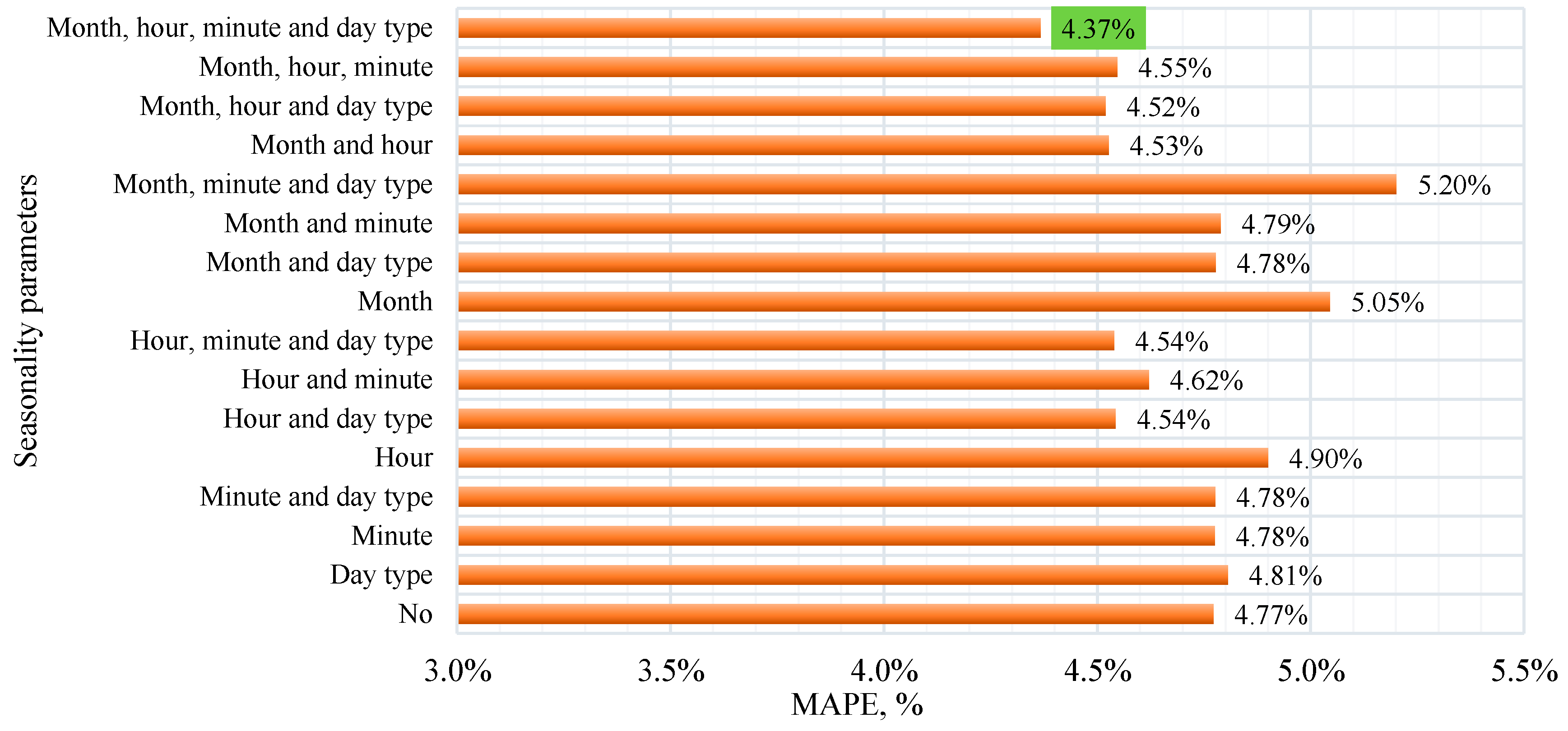
Figure 10.
The influence of seasonal components on the quality of the pressure forecasting model.
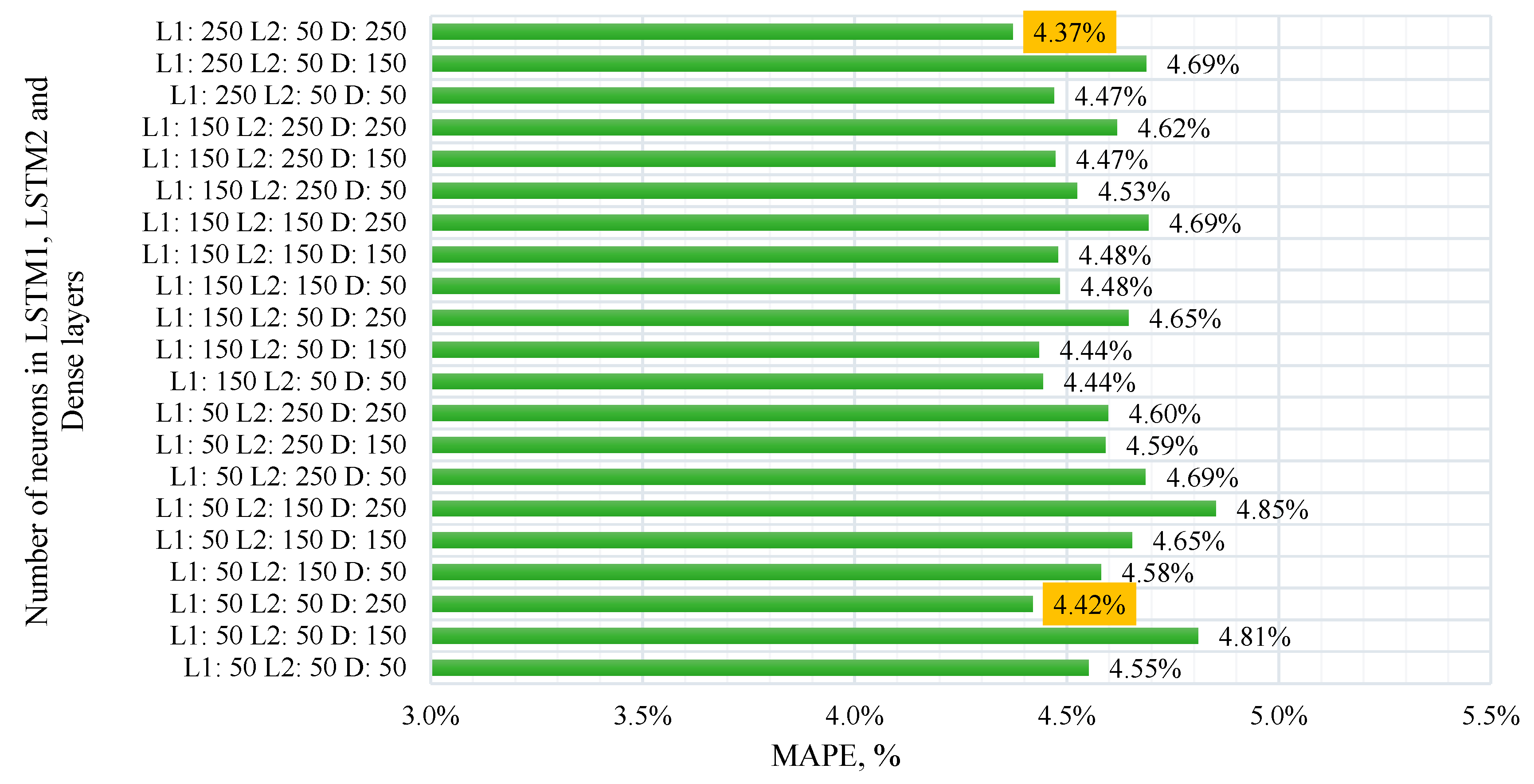
Figure 11.
The influence of history depth and forecast horizon length on model quality.
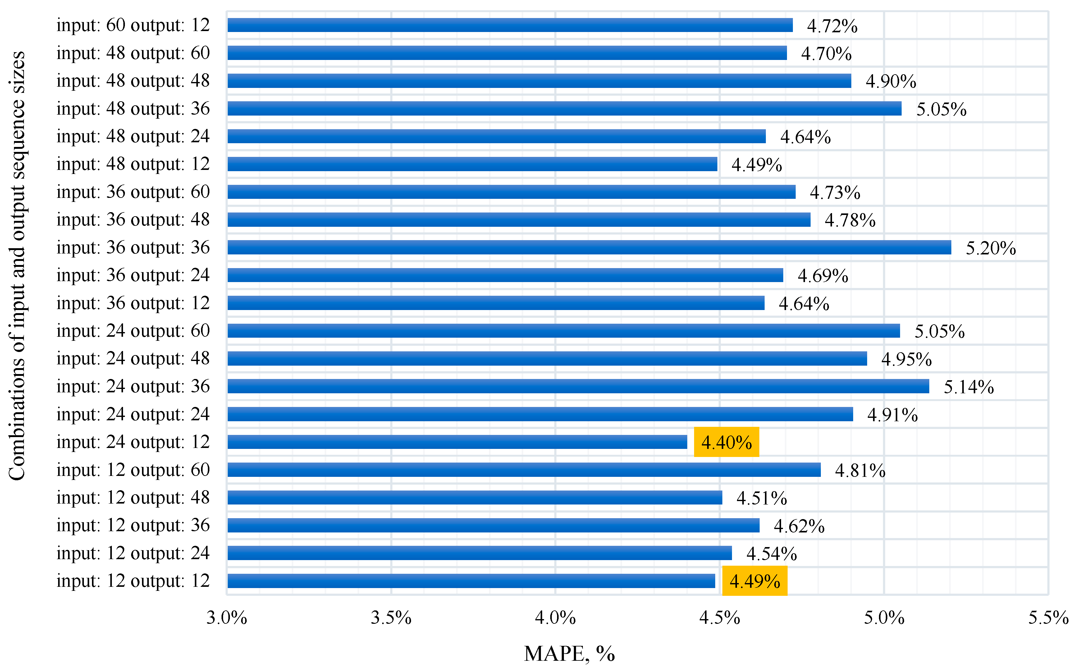
Figure 12.
Change in the mean square error (loss function) with increasing number of training epochs.
Figure 12.
Change in the mean square error (loss function) with increasing number of training epochs.
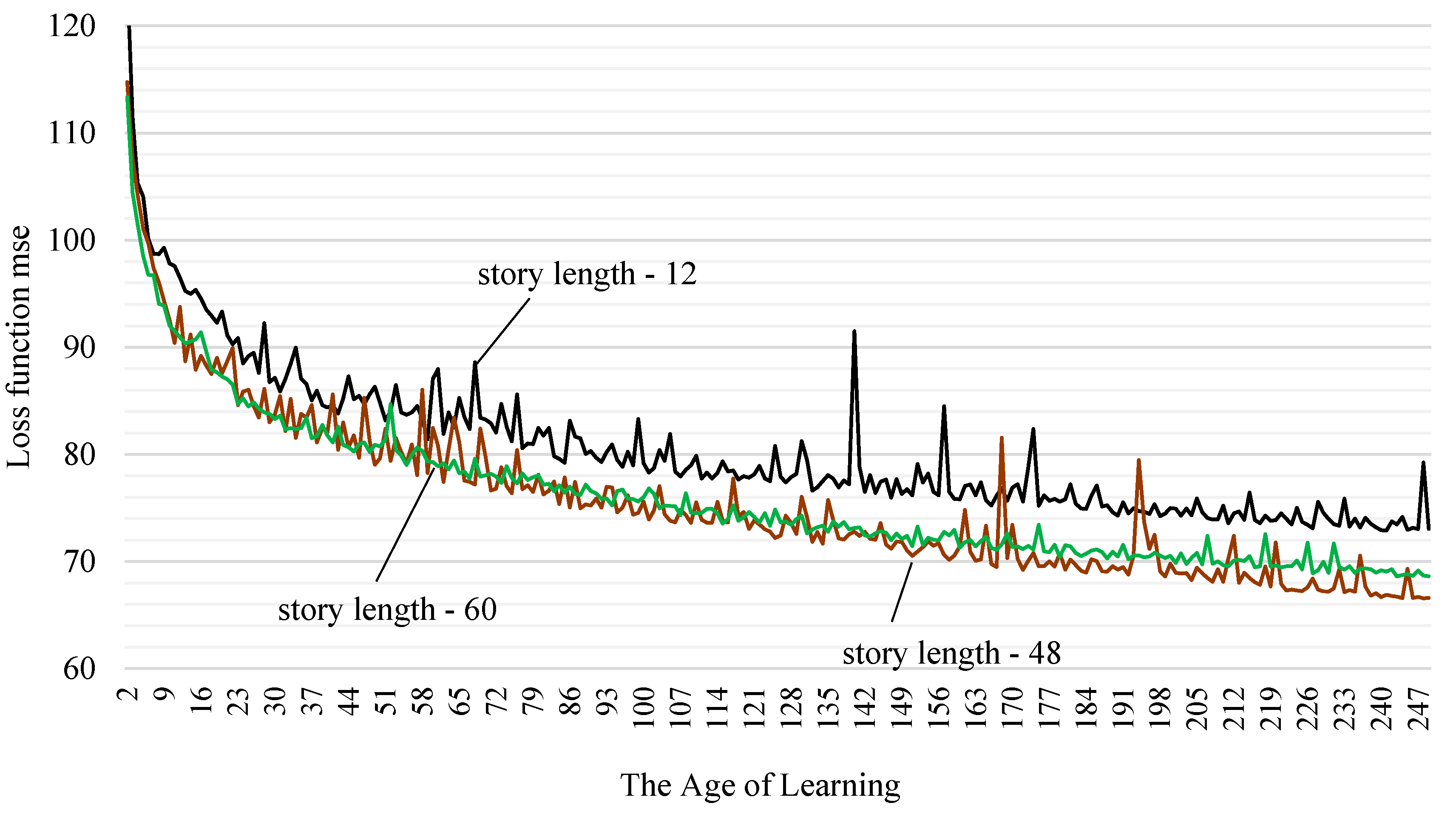
Figure 13.
Comparison of the Long Short-Term Memory Model with the Holt-Winters Model.
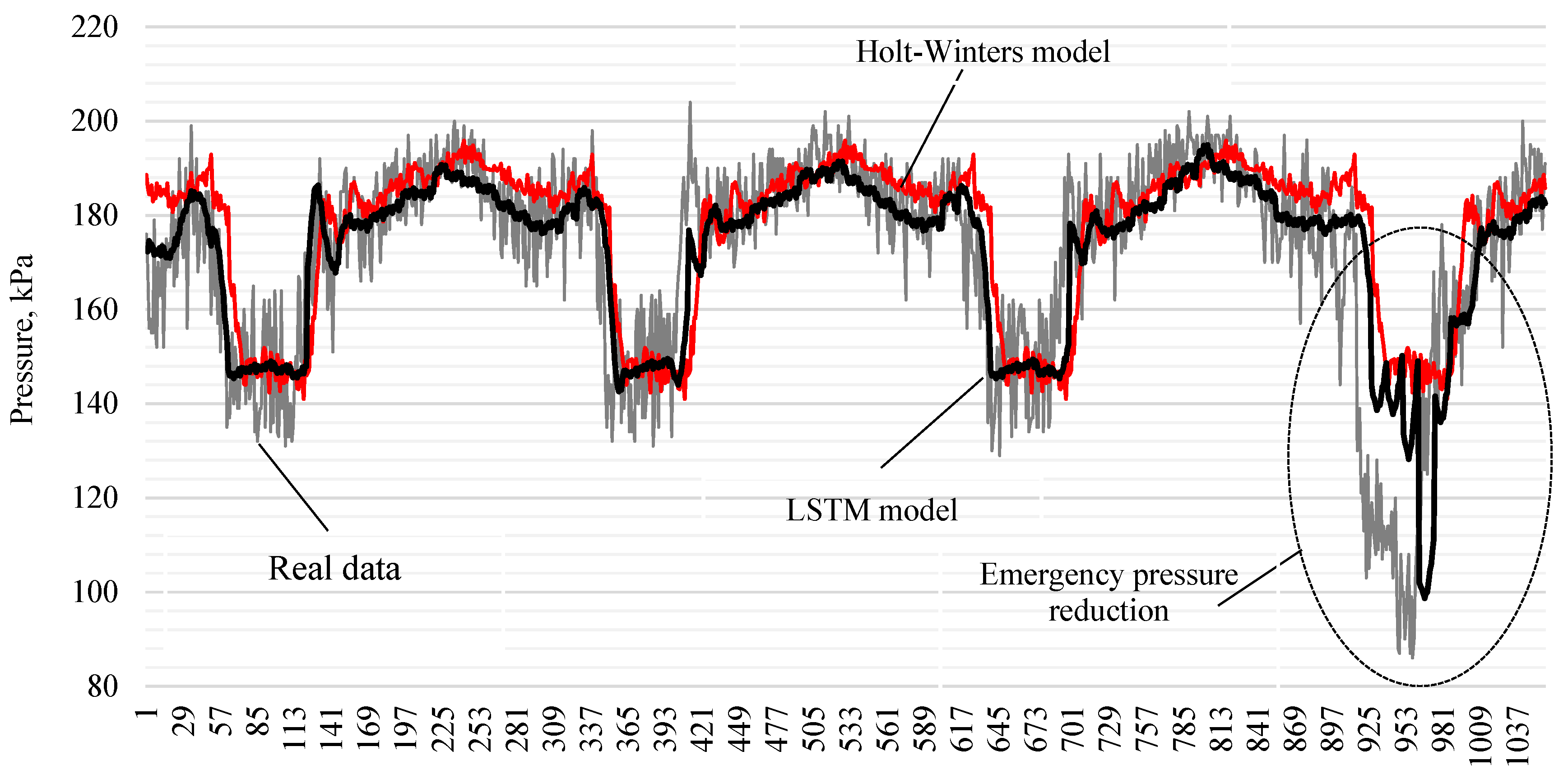

Table 1.
Simplified representation of pressure time series.
| Epoch (Unix time) | Pressure, kPa |
|---|---|
| 1662768000 | 156 |
| 1662768300 | 167 |
| 1662768600 | 168 |
| 1662768900 | 179 |
| ... | ... |
Disclaimer/Publisher’s Note: The statements, opinions and data contained in all publications are solely those of the individual author(s) and contributor(s) and not of MDPI and/or the editor(s). MDPI and/or the editor(s) disclaim responsibility for any injury to people or property resulting from any ideas, methods, instructions or products referred to in the content. |
© 2025 by the authors. Licensee MDPI, Basel, Switzerland. This article is an open access article distributed under the terms and conditions of the Creative Commons Attribution (CC BY) license (http://creativecommons.org/licenses/by/4.0/).
Copyright: This open access article is published under a Creative Commons CC BY 4.0 license, which permit the free download, distribution, and reuse, provided that the author and preprint are cited in any reuse.


