
Submitted:
30 April 2025
Posted:
30 April 2025
You are already at the latest version
Abstract
Accurate prediction of dissolved oxygen levels in river systems is essential for effective water quality management. A novel hybrid model combining Random Forest (RF) and Long Short-Term Memory (LSTM) networks is presented for dissolved oxygen forecasting in river ecosystems. The methodology utilizes RF to analyze feature importance and select relevant variables, reducing input dimensions and eliminating parameters with minimal influence on dissolved oxygen. LSTM networks then model the temporal relationships between the selected water quality parameters and dissolved oxygen levels. The model was validated using real-world river water quality data. Evaluation results show the RF-LSTM model achieves performance metrics of MSE (0.0028), RMSE (0.0529), MAE (0.0405) and R² (0.9890). The research demonstrates LSTM networks’ effectiveness for DO prediction and highlights the importance of data preprocessing and feature selection in environmental modeling.
Keywords:
Random Forest
; LSTM
; Water quality management
; dissolved oxygen prediction
; Yangtze River Basin
; machine learning
1. Introduction
Water is an indispensable resource for life on Earth. It is not only the core element for the normal functioning of ecosystems, but also plays a vital role in industrial production, agricultural activities, and human daily life. According to the China Water Resources Bulletin, the surface water supply reached 487.47 billion cubic meters, accounting for 82.5% of the total water supply [1], and has become the main source of drinking and domestic water for humans. In surface water bodies, the concentration of dissolved oxygen is not only closely related to the living environment of aquatic organisms, but also directly reflects the self-purification capacity and pollution status of the water body. When the DO concentration falls below critical thresholds, it can easily lead to hypoxia and odor formation, which seriously affects water quality safety. Therefore, accurate monitoring and prediction of dissolved oxygen concentration in water bodies have become key research areas in water environment protection and water quality management.
However, traditional DO prediction methods mainly rely on on-site monitoring and laboratory analysis, such as temperature-DO relationship models and biochemical oxygen demand models. These methods are constrained by limitations including sampling frequency, laboratory conditions, and environmental variability, making it difficult to achieve real-time and continuous prediction. Moreover, the relationship between DO concentration and multiple influencing factors, such as water temperature, pH, and turbidity, is complex and nonlinear, which traditional statistical methods struggle to effectively characterize [2,3].
In recent years, the rapid development of artificial intelligence technology has brought breakthroughs in DO prediction. With powerful nonlinear modeling capabilities, machine learning models can simultaneously process multiple influencing factors, explore the intrinsic patterns of DO variations from historical monitoring data, and significantly improve prediction accuracy and efficiency. Among these models, the long short-term memory (LSTM) network has demonstrated exceptional performance in DO time series prediction due to its unique gating mechanism and ability to model temporal dependencies.
DO concentration fluctuations are influenced by both natural conditions and human activities, exhibiting significant nonlinear and non-stationary characteristics. Accurate prediction of DO trends not only helps in the timely detection of water quality anomalies but also provides scientific support for water environment management and pollution control. Therefore, this study develops a dissolved oxygen prediction model based on LSTM using measured data from the Dujiangyan Water Quality Monitoring Station in the Yangtze River Basin. The objective is to enhance prediction accuracy and timeliness, thereby offering technical support for water quality early warning systems and management decision-making.
2. Related Work
Dissolved oxygen is a key indicator for water quality assessment and is essential for maintaining the health of aquatic ecosystems. The solubility of DO is dynamically affected by multiple factors, among which temperature is the main influencing factor and is significantly negatively correlated. In addition, atmospheric pressure, water pH, redox potential and the presence of pollutants can affect the solubility and transformation pathway of DO. The dynamic characteristics of DO show strong nonlinearity and time-varying properties. These complex change patterns put forward high technical requirements for its monitoring and prediction.
Internationally, the prediction method of dissolved oxygen has developed from statistical methods to machine learning. Early studies mainly relied on statistical methods such as multivariate linear regression, which can analyze the linear relationship between water quality parameters, but it is difficult to capture nonlinear relationships [4]. Subsequently developed empirical models, such as BP neural networks and Support Vector Machine (SVM), have made significant progress in dealing with nonlinear relationships. In recent years, deep learning models represented by LSTM have shown superiority in processing time series data [5] and have become the mainstream direction of water quality prediction research. In 2023, researchers applied LSTM to multivariate water quality prediction and achieved an R² of 0.86, which is significantly better than traditional methods [6].Studies have shown that LSTM performs exceptionally well in DO prediction for aquaculture and rivers, demonstrating notable advantages in capturing seasonal fluctuations and anomalous events, such as sudden pollution incidents [7,8].
In China, machine learning technology has been widely used in DO prediction research. The SVM model developed by researchers verified the model’s ability to effectively capture the nonlinear dynamic changes of DO[9,10], while [11]’s MTL-CNN-LSTM model demonstrated the superiority of deep learning technology in DO trend prediction.
Support vector machines use kernel functions to handle nonlinear relationships between water quality parameters and show strong generalization ability. The SVM model, combined with the optimization algorithm, has been successfully applied to DO prediction in rivers and reservoirs. Artificial neural networks use multi-layer perceptrons to achieve complex mappings between input and output, and can automatically learn complex patterns in data. Studies have shown that by optimizing input combinations, the determination coefficient of artificial neural network (ANN) in reservoir DO prediction can reach 0.98 [12].
Random forests [13] and extreme learning machines (ELM) [14] have also been applied to DO prediction. LSTM has shown strong time series modeling capabilities in comparison, and is particularly suitable for cross-seasonal or cross-year DO prediction tasks [15]. Studies have shown that deep learning models are generally superior to traditional machine learning models [16], and the R² of LSTM can reach 0.98, significantly higher than ANN’s 0.91 and SVM’s 0.77.
The prediction performance of LSTM model depends largely on data quality, feature selection and model parameter optimization [17]. The Z-score method effectively detects outliers in water quality data [18] and significantly improves the accuracy of DO prediction model. For missing data processing, various interpolation methods are applied [19], while data smoothing techniques help to eliminate short-term fluctuations and optimize LSTM input features [20].
In terms of feature selection, previous studies have shown that selecting the top correlated features significantly improves LSTM performance in predicting DO concentration [21]. Researchers used the maximum information coefficient analysis to find that conductivity, ammonia nitrogen and total nitrogen are the key features for DO prediction [22]. Another study used the SVR model to study DO prediction, and the results showed that pH and total phosphorus are also important influencing factors [23]. The researchers used the RF algorithm to analyze the key factors affecting DO changes [24], and the LSTM model combined with these insights improved the prediction accuracy by 15%. Other techniques such as PCA and LASSO [25,26] were also used for dimensionality reduction.
Hyperparameter optimization is a key factor in improving prediction accuracy. Intelligent optimization methods such as genetic algorithms [27], random search, and particle swarm optimization [28] have performed well in this area.
Most DO prediction studies focus on rivers, lakes, and aquaculture environments abroad [29], and these research results are difficult to directly apply to China’s complex hydrological environment, especially the Yangtze River Basin. This study fills the regional gap in China’s surface water prediction research by collecting and analyzing multidimensional water quality data from the Dujiangyan site, and provides technical support for China’s water quality monitoring and management system.
3. Materials and Methods
3.1. Study Area and Dataset Analysis
Dujiangyan is located in Sichuan Province, China, on the Min River at the western edge of the Chengdu Plain. It serves multiple comprehensive functions including agricultural irrigation, domestic water supply, flood control, aquaculture, and fisheries in the central and western parts of the Sichuan Basin, making it an irreplaceable water conservancy infrastructure in Sichuan Province [30]. The Min River is an important tributary in the upper reaches of the Yangtze River, with a watershed area of approximately 135,881 square kilometers and an average annual runoff of 89.6 billion cubic meters [31]. The Dujiangyan Environmental Monitoring Station regularly conducts water quality assessments at various cross-sections of the river. Figure 1 shows the geographical location of the Dujiangyan area and the monitoring stations used in this study.
The data utilized in this study were obtained from the Dujiangyan Water Quality Monitoring Station, accessed via the China Water Quality Monitoring Platform (https://szzdjc.cnemc.cn:8070/GJZ/Business/Publish/Main.html), a critical water source monitoring point situated in the Min River Basin, a part of the Yangtze River Basin system, in Chengdu, Sichuan Province.The monitoring data encompasses the entire year of 2023, spanning from January to December, with measurements recorded at 4-hour intervals. The dataset comprises nine core variables including DO, temperature, pH, and turbidity. A total of 1,911 sample records were collected, with each record containing multiple environmental parameters. The data exhibit time series characteristics with potential seasonal variations and diverse fluctuations. Preliminary analysis revealed the presence of occasional missing values and anomalies, necessitating subsequent data cleaning and rectification procedures. These variables encompass the primary physical, chemical, and biological characteristics influencing water quality, providing comprehensive data support for dissolved oxygen concentration prediction research. The key parameters involved in this study are shown in the Table 1.
Statistical analysis of the annual monitoring data from Dujiangyan water quality monitoring station in 2023 (as shown in the Figure 2) revealed significant distribution differences among water quality parameters. DO exhibited an annual mean of 9.52 mg/L, with a median of 9.53 mg/L and a standard deviation of 0.56 mg/L, demonstrating typical normal distribution characteristics. The distribution histogram shows DO values predominantly concentrated in the range of 9.0-10.0 mg/L, indicating that dissolved oxygen levels in the study area remained not only stable but also at an optimal level.Temperature, a critical parameter affecting DO, displayed pronounced multimodal distribution characteristics. The annual mean temperature was 13.89°C, with a median of 14.20°C and a standard deviation of 3.59°C, spanning an annual temperature range of 15°C (5-20°C). This multimodal distribution pattern accurately reflects the seasonal temperature variations in the study area, while also indicating that temperature fluctuations would significantly influence dissolved oxygen solubility.
3.2. Data Preprocessing
This research establishes a comprehensive framework for achieving high-precision predictions of dissolved oxygen concentrations in the Yangtze River Basin. Figure 3 illustrates the research framework. The methodology encompasses data collection, preprocessing, model design, training, and evaluation phases, ensuring scientific rigor and systematic approach throughout the study.
Based on statistic analysis, the dataset contains anomalous values likely resulting from sensor malfunctions or environmental fluctuations. To ensure data accuracy and reliable model inputs, this study implemented the Z-score method for outliers detection and flagging. The Z-score calculation is expressed as:
where x represents the sample value, denotes the sample mean, and represents the standard deviation. Data points with Z-scores exceeding the predetermined threshold (typically ) were flagged as anomalies and subsequently replaced with null values for treatment in missing value operations.
Following outliers detection, missing value treatment was implemented. The dataset exhibited both short-term and long-term data gaps due to monitoring station maintenance or operational constraints. For the dissolved oxygen data from Dujiangyan monitoring station, this study applied a stratified treatment approach: linear interpolation for short-term gaps (<3 days) and forward-backward filling for extended missing periods. For a missing data point y, the calculation formula is Equation 2:
Linear interpolation estimates missing values by constructing linear functions between adjacent temporal observations, effectively preserving data continuity and time series characteristics. This methodology enhanced data completeness while avoiding the bias associated with direct deletion. Additionally, a moving window smoothing technique with a window size of 6 was employed to mitigate noise effects on time series stationarity, effectively reducing short-term fluctuations while maintaining the underlying data trends.The moving average is calculated as shown in Equation 3:
where represents the smoothed value at the window center, n denotes the window size, and represents data points within the window.
3.3. Feature Importance Analysis
The Random Forest methodology was employed to analyze input variable importance for optimizing model features and enhancing dissolved oxygen concentration prediction accuracy. As an ensemble learning method combining multiple decision trees, Random Forest effectively handles non-linear relationships while quantifying feature contributions through various metrics. To ensure analytical reliability, multiple parameter configurations were systematically evaluated, including variations in the number of decision trees (10, 50, and 100) and maximum tree depths (10, 50, and 100). Feature importance scores were calculated as the average reduction in impurity when each feature serves as a splitting node across all trees, expressed as:
where represents the number of trees and denotes the impurity reduction caused by feature j in tree t.
The model training was repeated with each parameter combination, recording average rankings and standard deviations under different importance metrics, with particular attention paid to features maintaining high importance across configurations. This approach not only considers non-linear relationships between features and the target variable but also addresses feature interactions, providing reliable support for subsequent model construction.
3.4. Method Selection and Evaluation
In this study, to comprehensively evaluate dissolved oxygen prediction performance, SVM and ANN models were introduced for comparative analysis with the LSTM model. Both models employed hyperparameter optimization and cross-validation strategies to ensure optimal performance in prediction tasks.
SVM, based on structural risk minimization theory, effectively handles nonlinear problems and high-dimensional data. This study constructed an SVM model using the scikit-learn framework, evaluating both Radial Basis Function (RBF) and linear kernels to capture complex relationships among water quality parameters. To optimize performance, key hyperparameters were systematically explored: the penalty coefficient C ranged from 0.1 to 100, balancing model complexity and training error, while gamma values (’scale’, ’auto’, 0.1, 0.01) controlled the RBF kernel’s influence radius. The study employed RandomizedSearchCV with 50 iterations and TimeSeriesSplit (10-fold) cross-validation to maintain temporal dependencies and prevent data leakage. A fixed random seed (42) ensured reproducibility, providing a robust foundation for performance improvement. The parameter search ranges are detailed in Table 2.
ANN model was employed to process complex relationships between water quality parameters due to its strong feature learning capabilities. The model was constructed using the MLPRegressor from scikit-learn, leveraging the Rectified Linear Unit (ReLU) activation function to enhance non-linearity while mitigating the vanishing gradient problem. The model was trained using the Mean Squared Error (MSE) loss function, with systematic hyperparameter optimization. Hidden layer sizes of 50, 100, and 150 neurons were tested, evaluating both ReLU and Tanh activation functions. The learning rate was searched over the range [0.001, 0.01], and an L2 regularization parameter (alpha) in the range of [0.0001, 0.001] was applied to control complexity and prevent overfitting. The model was trained for 1,000 epochs, with hyperparameter tuning performed using RandomizedSearchCV (50 iterations) and evaluation using 10-fold time series cross-validation, ensuring temporal continuity for reliable performance assessment. The detailed parameter search ranges are presented in Table 3.
LSTM, a specialized variant of RNN , is renowned for its exceptional memory capabilities, making it particularly suitable for time series modeling and water quality prediction. Unlike traditional machine learning methods, LSTM effectively captures long-term dependencies in data, allowing it to model dynamic patterns in water quality parameters. The model’s core mathematical operations involve a forget gate, an input gate, a candidate memory gate, an output gate, and an updated hidden state, each playing a crucial role in maintaining information flow through time steps. The mathematical formulation is expressed as follows:
The forget gate is responsible for deciding which information to discard from the cell state:
The input gate determines which new information to update in the cell state:
The candidate memory gate calculates a new candidate value to be added to the cell state:
The output gate determines which information from the cell state is propagated to the hidden state:
The cell state is updated by combining the forget gate and input gate operations:
Finally, the hidden state is updated based on the output gate and the updated cell state:
The LSTM model was constructed based on the scikit-learn framework, with the overall network design comprising five main components:
- Input Layer: Receives preprocessed input feature data, providing foundational information for subsequent network layers.
- First LSTM Layer: Extracts long-term dependencies from time series data, capturing dynamic data characteristics.
- Second LSTM Layer: Further explores deep temporal dependency features, enhancing model expressiveness.
- Dropout: Implements regularization with a specified dropout rate, reducing overfitting risk through random deactivation of neurons during training.
- Output Layer: A fully connected layer mapping previous layer outputs to target variables, generating final predictions.
To optimize model performance, hyperparameter tuning was conducted using random search, which efficiently explores the parameter space compared to traditional grid search by reducing computational costs while maintaining accuracy. The hyperparameter space included LSTM layer units ([32, 128]), number of LSTM layers, dropout rate ([0.1, 0.5]), activation functions (ReLU, Tanh), and learning rate ([0.001, 0.01]). This systematic tuning approach ensured robust model performance while mitigating overfitting, with detailed parameter search ranges presented in Table 4.
To comprehensively evaluate the prediction performance of the LSTM model, this study employs four key evaluation metrics: Mean Absolute Error (MAE), Mean Squared Error (MSE), Root Mean Squared Error (RMSE), and the Coefficient of Determination (). MAE measures the average magnitude of prediction errors, with lower values indicating higher accuracy. MSE, which calculates the average squared deviation between predicted and actual values, is particularly sensitive to large errors, making it crucial for assessing overall prediction performance. RMSE, as the square root of MSE, maintains the same unit as the original data, providing an interpretable measure of the model’s standard deviation in prediction errors. Lastly, quantifies the proportion of variance explained by the model, with values closer to 1 indicating a better fit and higher predictive power. These metrics collectively assess absolute error, squared error, and explanatory power, ensuring a comprehensive evaluation of the model’s accuracy and robustness.
4. Results and Discussion
The experiments were conducted using Python 3.11.5 and a stable set of libraries (Pandas, NumPy, Matplotlib, Seaborn, Scikit-learn, TensorFlow, Keras, and Keras-tuner) to support efficient data processing, model construction, and hyperparameter optimization, with reproducibility ensured by fixed library versions and random seed control. This chapter presents a comprehensive analysis of experimental results for the Dujiangyan dissolved oxygen prediction method. Using 1,911 preprocessed records from the Dujiangyan monitoring station, we first examined feature importance rankings before evaluating the model across multiple performance metrics. Results demonstrate that our proposed method effectively captures complex temporal patterns and environmental factors influencing dissolved oxygen concentrations, achieving notable improvements in both prediction accuracy and stability.
4.1. Feature Importance Analysis Results
The feature importance analysis of the 9 features in the dataset of this study was performed to find the key factors that have the most significant impact on the change of dissolved oxygen concentration. Multiple Random Forest models were constructed by adjusting the maximum depth (max_depth=10, 50, 100) and the number of decision trees (n_estimators=10, 50, 100) to ensure the stability and reliability of the analysis results.
As shown in Figure 4 and Figure 5, the feature importance scores indicate that turbidity (importance score: ), conductivity (), and temperature () are the top three factors influencing DO variations. These findings align well with the physicochemical mechanisms governing dissolved oxygen dynamics in water bodies:
Changes in turbidity have a significant impact on dissolved oxygen in water. Increased turbidity reduces water transparency, inhibits photosynthesis of aquatic plants, and thus affects oxygen production. In addition, a large amount of suspended particles carried by heavy rain or surface runoff into rivers will disturb the water environment and cause short-term fluctuations in dissolved oxygen concentration.
Conductivity reflects the concentration of dissolved ions and overall ionic strength in water, and can indirectly characterize changes in pollutant input or water self-purification capacity. Therefore, conductivity is often used as an important indicator for monitoring water quality changes.
Water temperature is one of the important factors affecting dissolved oxygen concentration. A large number of experimental studies and time series trend analysis have confirmed that there is a significant negative correlation between dissolved oxygen and water temperature. In the hot season (usually July to September), the dissolved oxygen concentration is generally low, which is consistent with the physical law that the solubility of gases decreases with increasing temperature.
In addition, pH exhibited a relatively lower importance score (), but maintained stability throughout the year, indicating the strong buffering capacity of the water body. Nutrient indicators, such as ammonia nitrogen (), total phosphorus (), and total nitrogen (), showed lower importance scores, suggesting that in the study area, DO variations are mainly driven by physical factors and short-term hydrological disturbances, while chemical factors have less influence.
Based on these results, parameters with importance scores greater than 0.1 (turbidity, conductivity, temperature, and pH) were selected as the input features for the DO prediction models. This selection not only ensures the representativeness of the model inputs but also reduces model complexity, providing a solid foundation for subsequent LSTM model construction and optimization.
4.2. Model Training Results Analysis
Model training was conducted using Python-based deep learning frameworks, primarily TensorFlow and Keras, to leverage their robust support for sequential data modeling. SVM, ANN, and LSTM models were trained on the preprocessed and standardized dataset, which included key water quality parameters such as DO, temperature, pH, turbidity, and conductivity. The dataset was split into a training set and a test set in an 80:20 ratio based on chronological order to ensure sufficient sample size for model training and validation.
The hyperparameter optimization for the SVM, ANN, and LSTM models was conducted using a random search approach. Table 5 summarizes the optimal hyperparameter configurations identified for each model. After obtaining the optimal parameters, we refit each model using these parameters and perform evaluation using 10-fold cross validation. Table 6 shows the comparison of the evaluation results of the three models.
4.3. SVM Model Performance
The SVM model exhibited excellent prediction performance, achieving an of 0.9888, indicating it could explain 98.88% of the observed variation. The model achieved a low MAE of 0.0371 mg/L, an MSE of 0.0029, and an RMSE of 0.0534 mg/L, demonstrating high prediction accuracy.
As shown in Figure 6, the SVM model accurately captured the dynamic fluctuations of dissolved oxygen concentrations. The prediction curve closely matched measured values, including sudden changes (notably around time point 1000). The scatter plot shows a tight linear correlation between predicted and observed values, with points closely distributed along the diagonal line, confirming strong prediction reliability.
The SVM model showed high concordance with measured values and maintained good tracking performance even during sudden concentration changes. This indicates strong environmental dynamic response capability and resistance to interference. The tight distribution of data points around the diagonal line in the scatter plot further validated the model’s reliability.
Compared with traditional time series prediction methods, the SVM model shows significant advantages in dealing with dissolved oxygen changes under the influence of nonlinear relationships and complex environmental factors. This may be attributed to the ability of the SVM kernel function to map data into a high-dimensional feature space, thereby effectively capturing the complex nonlinear relationships between water quality parameters. Despite the excellent performance of the model, it should be noted that its applicability may be limited under extreme climatic conditions (such as sudden heavy rains or long-term droughts). In addition, the generalization ability of the model also depends on the representativeness and completeness of the training data, if applied to water bodies with significantly different hydrological characteristics, retraining or parameter adjustment may be required. Future research may consider integrating more environmental factors, such as algal biomass, organic matter load, etc., to further improve the prediction accuracy and robustness of the model in complex water environments.
4.4. ANN Model Performance
The ANN model also demonstrated good predictive performance. The model achieved an of 0.9541, an MAE of 0.0719 mg/L, and an RMSE of 0.1079 mg/L, indicating reliable but slightly less accurate predictions compared to the SVM model.
As illustrated in Figure 7, the ANN model effectively captured DO dynamics, although a slight response lag was observed during rapid fluctuations. The scatter plot shows a clear linear correlation between predicted and measured values, with slightly larger deviations in the high-concentration range, suggesting that the ANN model’s generalization ability under extreme conditions could be further improved.
Although the ANN model can effectively capture the overall trend, it shows a slight response lag during periods of dramatic fluctuations. This phenomenon may be attributed to the learning characteristics of the neural network in dealing with nonlinear relationships. The scatter plot shows that the prediction accuracy decreases in high-concentration areas, indicating that the model has limited generalization ability under extreme conditions. The hysteresis response characteristics exhibited by the ANN model may be related to its mechanism for processing time series data. Compared with SVM, ANN may overfit specific patterns in the training data during the weight adjustment process, resulting in insufficient sensitivity to emerging mutation responses. This finding suggests that we should consider the matching degree between the model response characteristics and the monitoring objectives in practical applications, especially in scenarios with high timeliness requirements such as water quality mutation monitoring.
4.5. LSTM Model Performance
The LSTM model demonstrated the best overall performance among the three models. The training process (Figure 8) exhibited a smooth convergence trend, with minimal differences between the training loss and validation loss curves, indicating that the model did not suffer from overfitting. The LSTM model achieved an value of 0.9890, a MAE of 0.0405 mg/L, a MSE of 0.0028, and a RMSE of 0.0529 mg/L, confirming its superior prediction accuracy.
The time series prediction results (Figure 9) show that the LSTM model can accurately track both stable trends and rapid fluctuations in dissolved oxygen concentration. The unique gating mechanisms of the LSTM, including the input gate, forget gate, and output gate, enable it to effectively handle temporal dependencies while maintaining sensitivity to sudden changes. The scatter plots further validate this performance, with predicted values closely aligned with measured values across the entire concentration range, reflecting the model’s stable performance under various conditions.
Compared to traditional models, the LSTM architecture significantly outperforms SVM and ANN models in handling nonlinear relationships and long-term temporal dependencies. Its memory cells are capable of storing and utilizing historical information over long sequences, which is particularly important for capturing seasonal patterns and long-term trends. This highlights the applicability of LSTM in complex environmental time series forecasting and its potential value in intelligent water quality monitoring and early warning systems. Future studies may explore integrating LSTM with other feature extraction techniques or developing hybrid model architectures to further enhance prediction performance and generalization ability.
5. Conclusion
This study addresses the challenge of DO prediction in river water quality monitoring by establishing a complete technical framework, including data preprocessing, feature selection, and multi-model evaluation. A differentiated strategy for handling missing data and a multi-combination feature validation approach were proposed to improve data quality and model performance.
Experimental results demonstrated that the LSTM model outperformed SVM and ANN in terms of accuracy and stability. All three models showed robust and reliable prediction capabilities through 10-fold cross-validation.
The contributions of this study are threefold:
- Theoretical Contribution: This work enhances the understanding of the temporal and spatial characteristics of water quality parameters and validates the applicability of deep learning techniques in DO prediction.
- Methodological Contribution: A systematic data preprocessing scheme and a Random Forest-based feature selection strategy were developed, along with a comprehensive multi-model comparison framework.
- Practical Contribution: The proposed models and methods can be applied in real-world water quality monitoring systems and provide technical support for water environment management and early warning systems.
Despite these achievements, limitations remain in data representativeness, model integration, and the consideration of environmental factors. Future research will focus on expanding spatiotemporal data coverage, exploring ensemble modeling, integrating additional influencing factors, and developing practical early warning applications.
In summary, this study provides an effective and systematic approach for dissolved oxygen prediction in river water and offers valuable references for intelligent water quality monitoring and management.
Author Contributions
Conceptualization and review framework, Z.O.; original draft preparation and writing, Y.W.; review and editing, Y.W., Z.O.; supervision, Z.O. All authors have read and agreed to the published version of the manuscript.
Funding
This research received no external funding.
Data Availability Statement
Not applicable.
Conflicts of Interest
The authors declare no conflicts of interest.
References
- Ministry of Water Resources of the People’s Republic of China. (2024, June 14). 2023 China Water Resources Bulletin released. Available online: https://www.chinawater.com.cn/yw/202406/t20240614_1052624.html (accessed on 23 March 2025).
- Tung, Tran Minh, Yaseen, Zaher Mundher, others (2020). A survey on river water quality modelling using artificial intelligence models: 2000–2020. Journal of Hydrology, 585(), 124670. [CrossRef]
- Siami-Namini, S., Tavakoli, N., & Namin, A. S. (2018, December). A comparison of ARIMA and LSTM in forecasting time series. In 2018 17th IEEE International Conference on Machine Learning and Applications (ICMLA) (pp. 1394–1401). IEEE. [CrossRef]
- Cox, B. A. (2003). A review of dissolved oxygen modelling techniques for lowland rivers. Science of the Total Environment, 314, 303–334. [CrossRef]
- Liu, Y., Zhang, Q., Song, L., Chen, Y. (2019). Attention-based recurrent neural networks for accurate short-term and long-term dissolved oxygen prediction. Computers and Electronics in Agriculture, 165, 104964. [CrossRef]
- Pyo, J.; Pachepsky, Y.; Kim, S.; Abbas, A.; Kim, M.; Kwon, Y. S.; ... Cho, K. H. (2023). Long short-term memory models of water quality in inland water environments. Water Research X, 21, 100207. [CrossRef]
- Khabusi, S. P., Huang, Y. P. (2022, August). A deep learning approach to predict dissolved oxygen in aquaculture. In 2022 International Conference on Advanced Robotics and Intelligent Systems (ARIS) (pp. 1–6). IEEE. [CrossRef]
- Pan, D., Zhang, Y., Deng, Y., Van Griensven Thé, J., Yang, S. X., Gharabaghi, B. (2024). Dissolved oxygen forecasting for Lake Erie’s central basin using hybrid long short-term memory and gated recurrent unit networks. Water, 16(5), 707. [CrossRef]
- Ji, X.; Shang, X.; Dahlgren, R. A.; Zhang, M. (2017). Prediction of dissolved oxygen concentration in hypoxic river systems using support vector machine: a case study of Wen-Rui Tang River, China. Environmental Science and Pollution Research, 24, 16062–16076. [CrossRef]
- Nong, X., Lai, C., Chen, L., Shao, D., Zhang, C., Liang, J. (2023). Prediction modelling framework comparative analysis of dissolved oxygen concentration variations using support vector regression coupled with multiple feature engineering and optimization methods: A case study in China. Ecological Indicators, 146, 109845. [CrossRef]
- Wu, X.; Zhang, Q.; Wen, F.; Qi, Y. (2022). A water quality prediction model based on multi-task deep learning: a case study of the Yellow River, China. Water, 14(21), 3408. [CrossRef]
- Ziyad Sami, B. F.; Latif, S. D.; Ahmed, A. N.; Chow, M. F.; Murti, M. A.; Suhendi, A.; ... El-Shafie, A. (2022). Machine learning algorithm as a sustainable tool for dissolved oxygen prediction: a case study of Feitsui Reservoir, Taiwan. Scientific Reports, 12(1), 3649. [CrossRef]
- Ruan, J.; Cui, Y.; Song, Y.; Mao, Y. (2023). A novel RF-CEEMD-LSTM model for predicting water pollution. Scientific Reports, 13(1), 20901. [CrossRef]
- Heddam, S.; Kisi, O. (2017). Extreme learning machines: a new approach for modeling dissolved oxygen (DO) concentration with and without water quality variables as predictors. Environmental Science and Pollution Research, 24(20), 16702–16724. [CrossRef]
- Li, W.; Wu, H.; Zhu, N.; Jiang, Y.; Tan, J.; Guo, Y. (2021). Prediction of dissolved oxygen in a fishery pond based on gated recurrent unit (GRU). Information Processing in Agriculture, 8(1), 185–193. [CrossRef]
- Moghadam, S. V.; Sharafati, A.; Feizi, H.; Marjaie, S. M. S.; Asadollah, S. B. H. S.; Motta, D. (2021). An efficient strategy for predicting river dissolved oxygen concentration: application of deep recurrent neural network model. Environmental Monitoring and Assessment, 193, 1–18. [CrossRef]
- Liu, P.; Wang, J.; Sangaiah, A. K.; Xie, Y.; Yin, X. (2019). Analysis and prediction of water quality using LSTM deep neural networks in IoT environment. Sustainability, 11(7), 2058. [CrossRef]
- Kulanuwat, L.; Chantrapornchai, C.; Maleewong, M.; Wongchaisuwat, P.; Wimala, S.; Sarinnapakorn, K.; Boonya-Aroonnet, S. (2021). Anomaly detection using a sliding window technique and data imputation with machine learning for hydrological time series. Water, 13(13), 1862. [CrossRef]
- Chen, Y.; Song, L.; Liu, Y.; Yang, L.; Li, D. (2020). A review of the artificial neural network models for water quality prediction. Applied Sciences, 10(17), 5776. [CrossRef]
- Eze, E.; Ajmal, T. (2020). Dissolved oxygen forecasting in aquaculture: A hybrid model approach. Applied Sciences, 10(20), 7079. [CrossRef]
- Elkiran, G., Nourani, V., Abba, S. I., Abdullahi, J. (2018). Artificial intelligence-based approaches for multi-station modelling of dissolve oxygen in river. Global Journal of Environmental Science and Management, 4(4), 439–450.
- Zhang, P.; Liu, X.; Dai, H.; Shi, C.; Xie, R.; Song, G.; Tang, L. (2024). A multi-model ensemble approach for reservoir dissolved oxygen forecasting based on feature screening and machine learning. Ecological Indicators, 166, 112413. [CrossRef]
- Liu, W.; Lin, S.; Li, X.; Li, W.; Deng, H.; Fang, H.; Li, W. (2024). Analysis of dissolved oxygen influencing factors and concentration prediction using input variable selection technique: A hybrid machine learning approach. Journal of Environmental Management, 357, 120777. [CrossRef]
- Huan, J.; Chen, B.; Xu, X. G.; Li, H.; Li, M. B.; Zhang, H. (2021). River dissolved oxygen prediction based on random forest and LSTM. Applied Engineering in Agriculture, 37(5), 901–910. [CrossRef]
- Tan, W.; Zhang, J.; Liu, X.; Yu, Z.; Xiao, K.; Wang, L.; ... Guo, P. (2022, September). Dissolved oxygen prediction based on PCA-LSTM. In Journal of Physics: Conference Series (Vol. 2337, No. 1, p. 012012). IOP Publishing. [CrossRef]
- Taşan, S. (2023). Estimation of groundwater quality using an integration of water quality index, artificial intelligence methods and GIS: Case study, Central Mediterranean Region of Turkey. Applied Water Science, 13(1), 15. [CrossRef]
- Singh, P.; Kaur, P. D. (2017). Review on data mining techniques for prediction of water quality. International Journal of Advanced Research in Computer Science, 8(5).
- Huang, M.; Hu, B. Q.; Jiang, H.; Fang, B. W. (2023). A water quality prediction method based on k-nearest-neighbor probability rough sets and PSO-LSTM. Applied Intelligence, 53(24), 31106–31128. [CrossRef]
- Yang, J. (2023). Predicting water quality through daily concentration of dissolved oxygen using improved artificial intelligence. Scientific Reports, 13(1), 20370. [CrossRef]
- Baidu Baijiahao. (2023). Sichuan Dujiangyan: Water conservancy for thousands of years, nourishing Sichuan. Available online: https://baijiahao.baidu.com/s?id=1823006260704459232&wfr=spider&for=pc (accessed on 23 March 2025).
- Baidu Baike. (2024). Dujiangyan. Available online: https://baike.baidu.com/item/%E9%83%BD%E6%B1%9F%E5%A0%B0/122963 (accessed on 23 March 2025).
Figure 1.
Dujiangyan Station Geographical Location
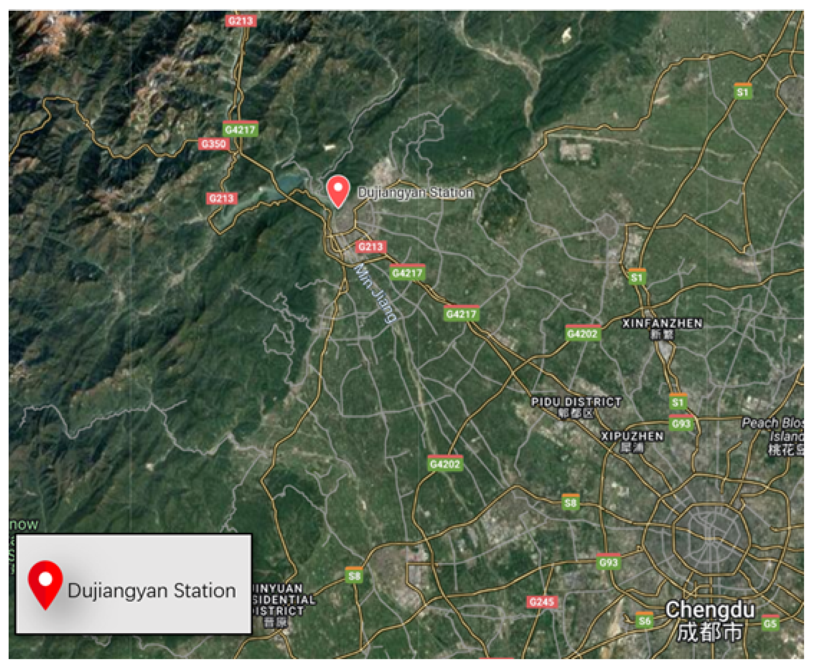
Figure 2.
Parameter Data Statistics
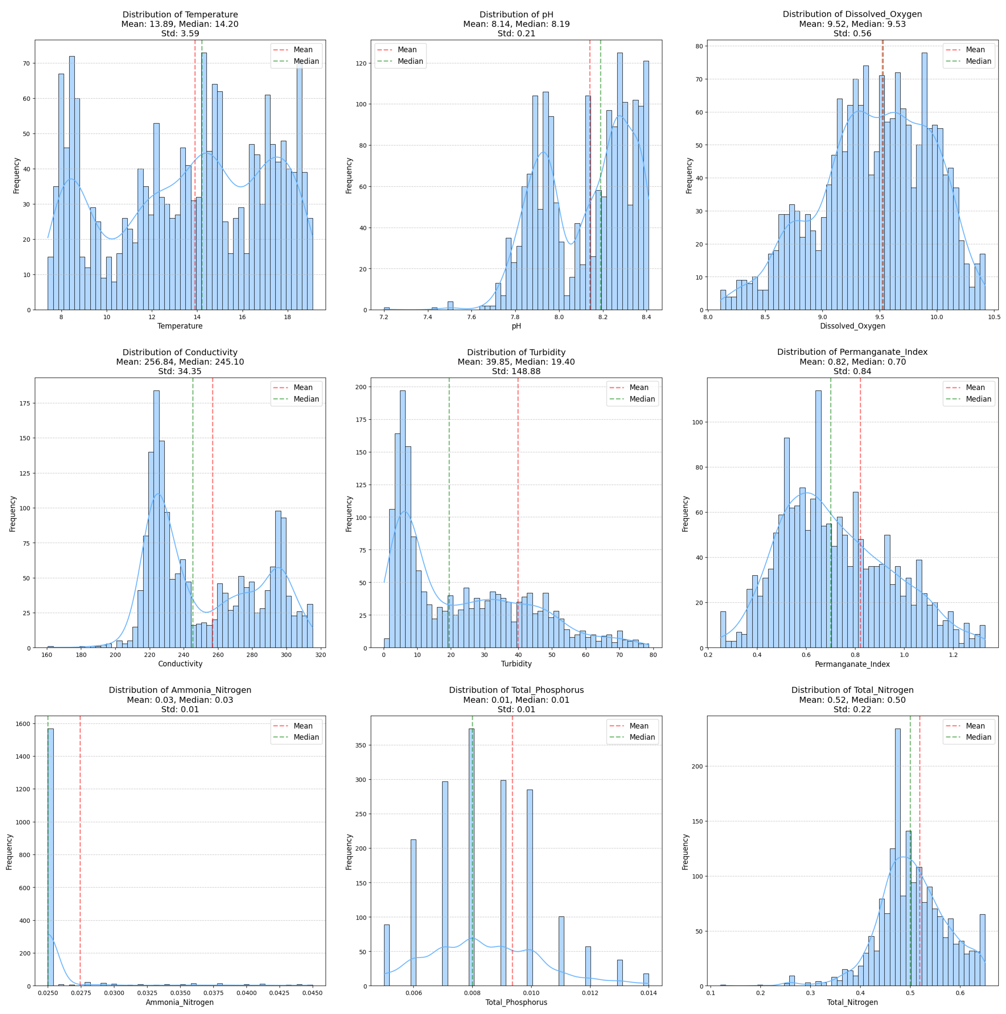
Figure 3.
Research Framework
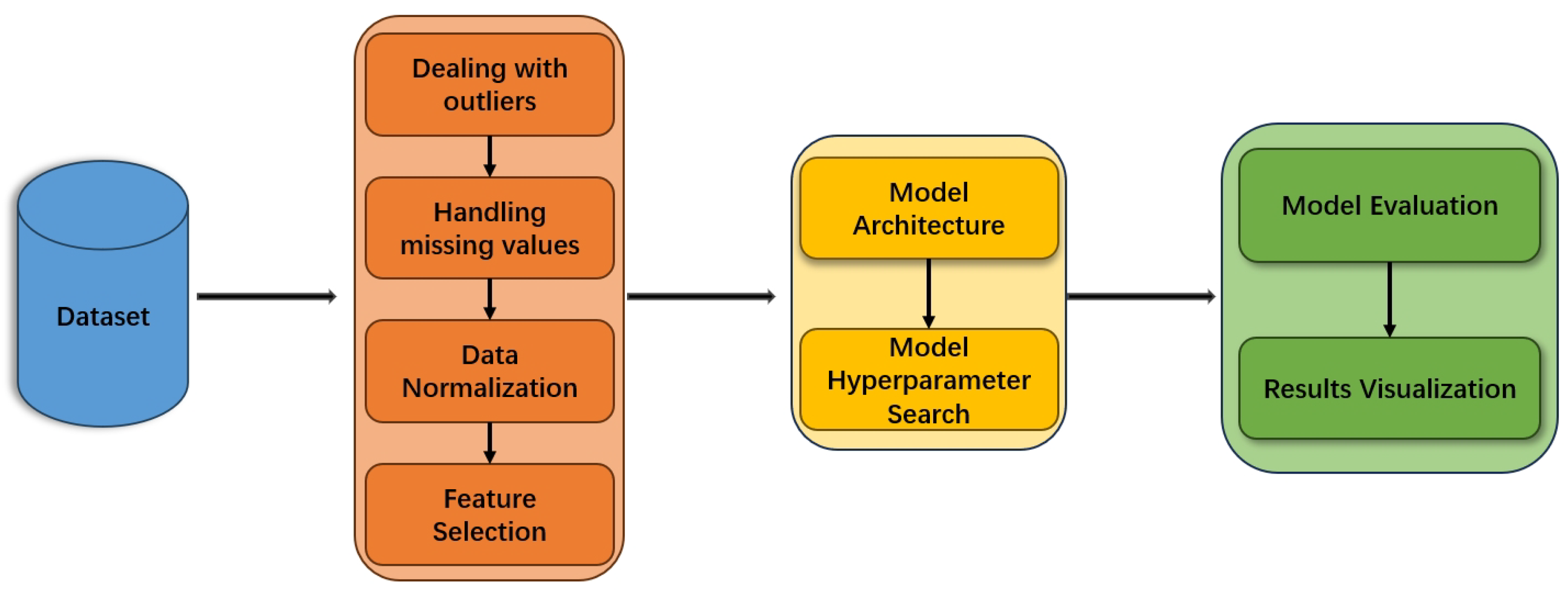
Figure 4.
Feature Importance Heatmap for Different Parameter Combinations
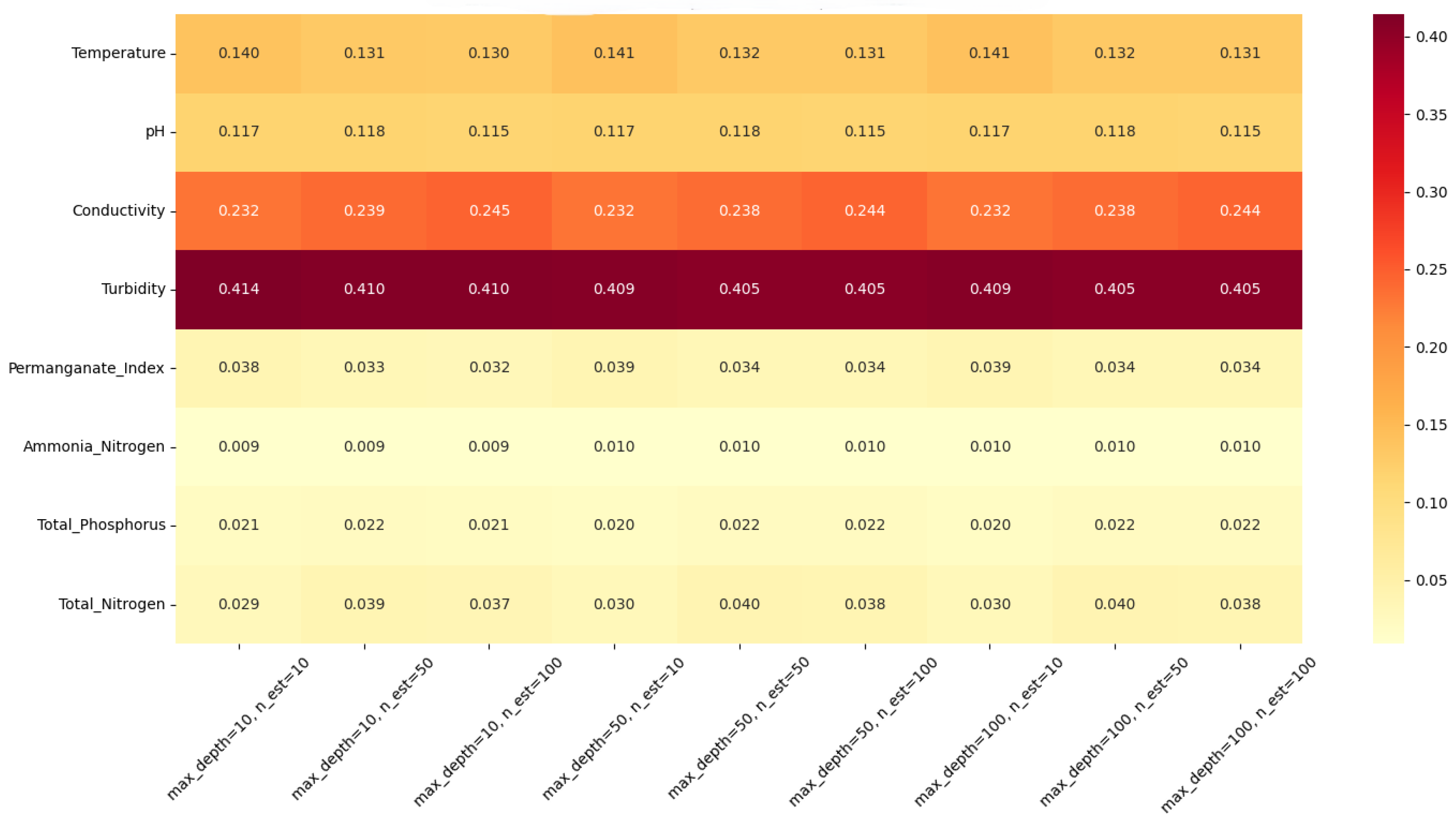
Figure 5.
Feature Importance Mean and Standard Deviation
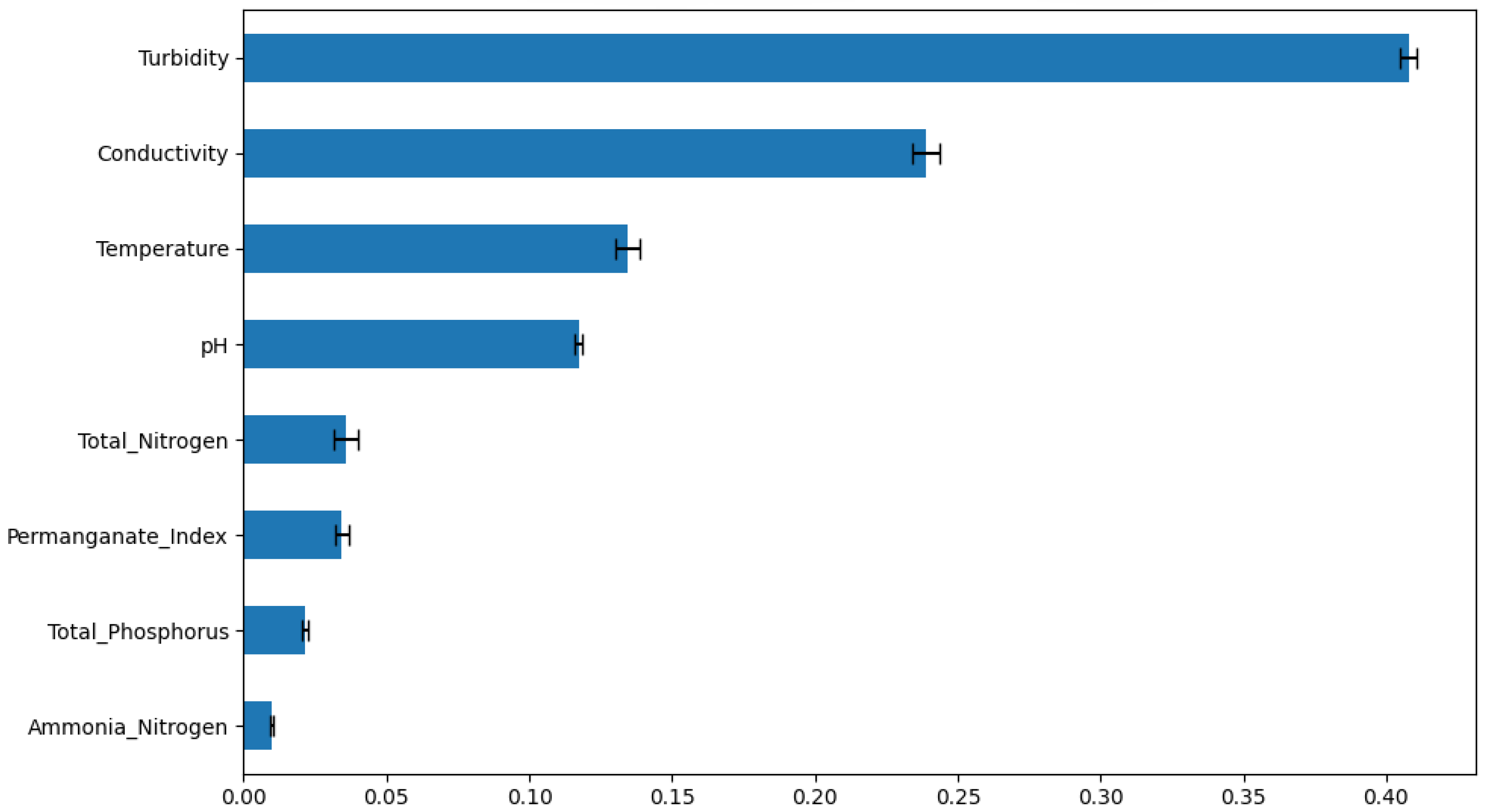
Figure 6.
Overview of SVM model analysis results: (a) SVM model prediction results. (b) SVM Scatter Plot.
Figure 6.
Overview of SVM model analysis results: (a) SVM model prediction results. (b) SVM Scatter Plot.
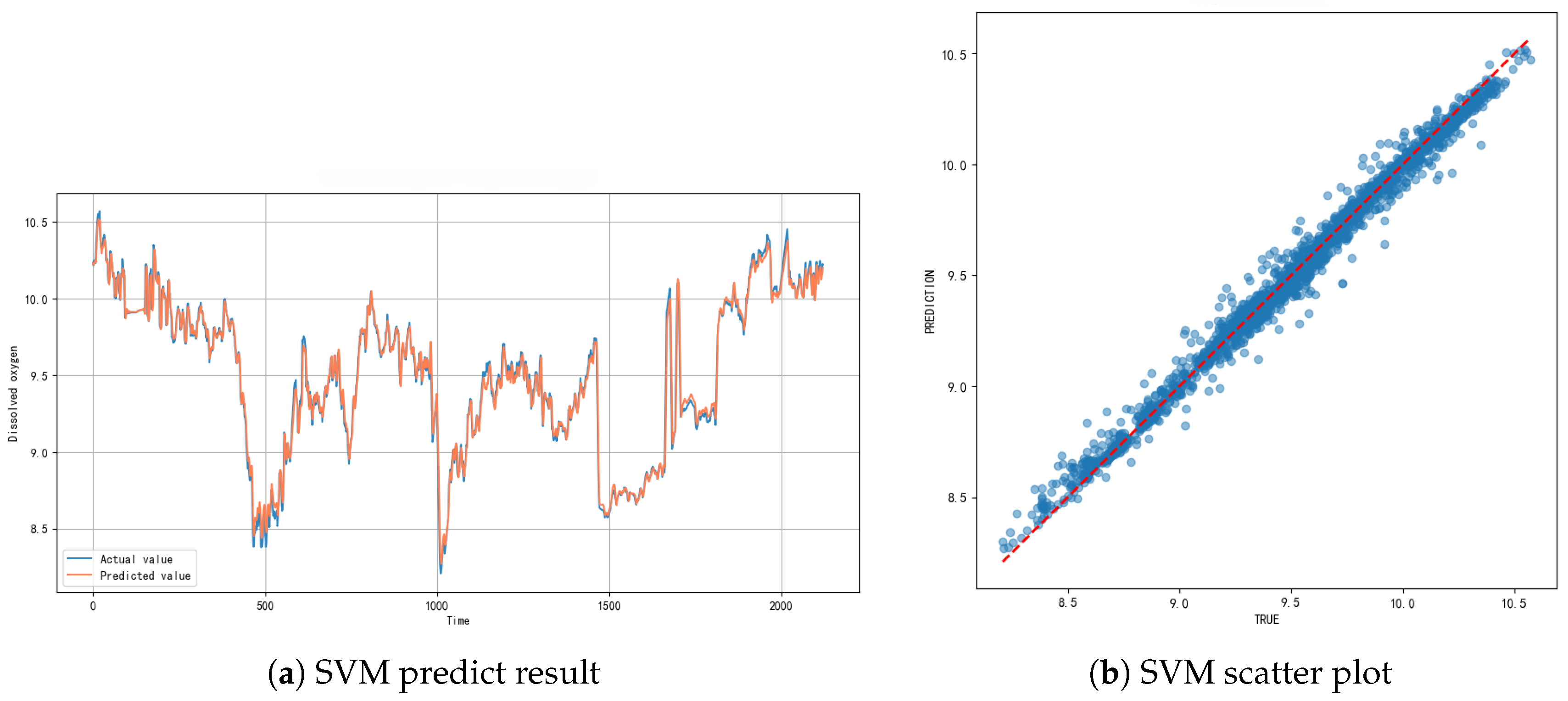
Figure 7.
Overview of ANN model analysis results: (a) ANN model prediction results. (b) ANN Scatter Plot.
Figure 7.
Overview of ANN model analysis results: (a) ANN model prediction results. (b) ANN Scatter Plot.
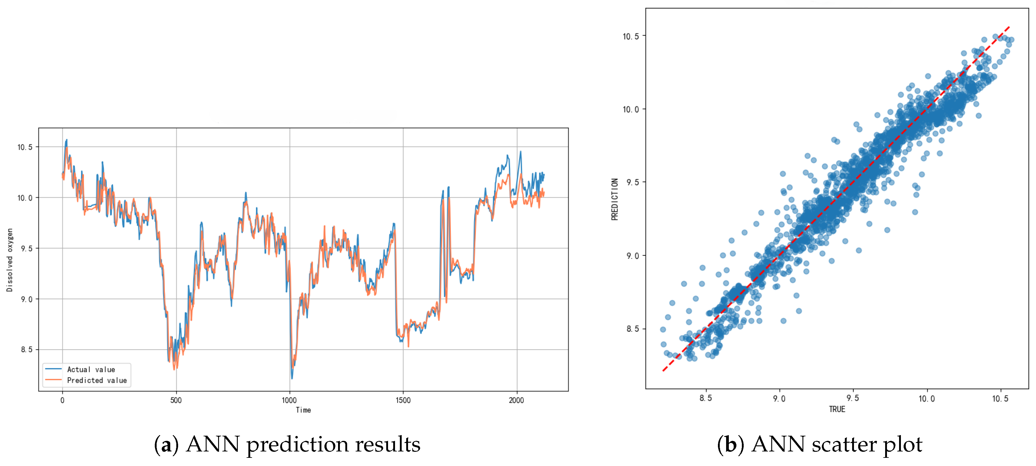
Figure 8.
LSTM Model Training Process
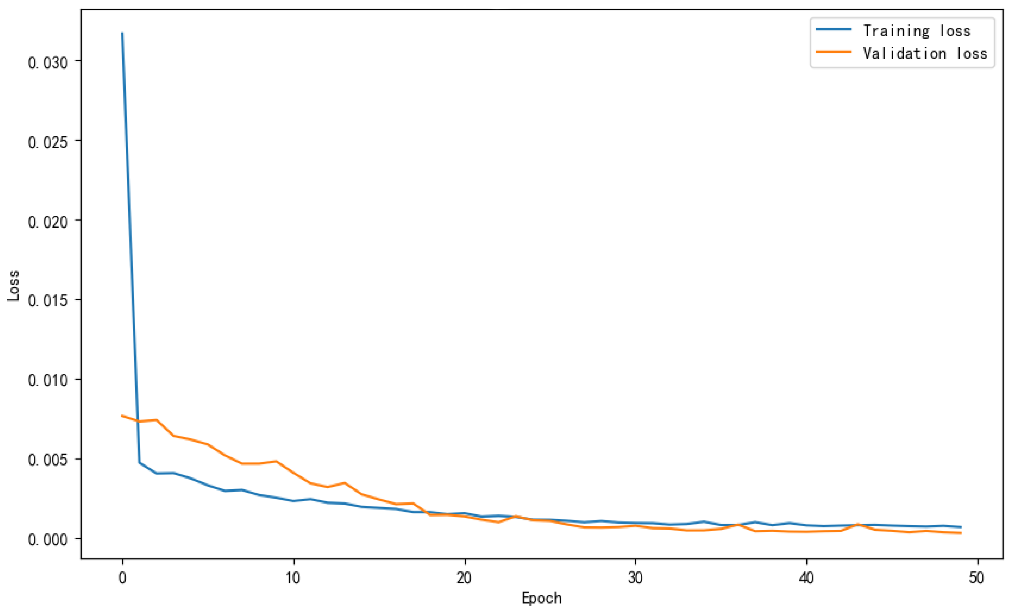
Figure 9.
Overview of LSTM model analysis results: (a) LSTM model prediction results. (b) LSTM Scatter Plot.
Figure 9.
Overview of LSTM model analysis results: (a) LSTM model prediction results. (b) LSTM Scatter Plot.
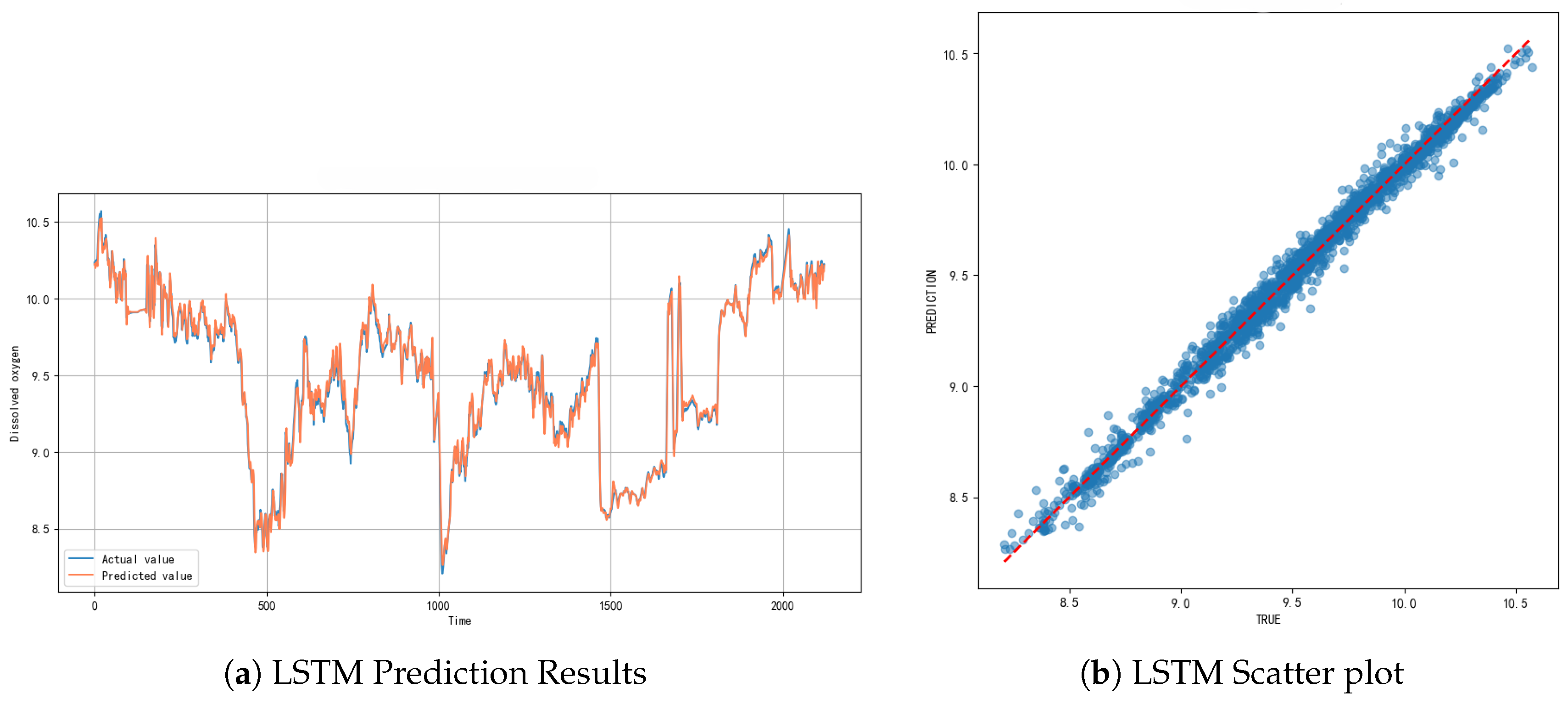

Table 1.
Description of Key Parameters in the Dataset
| Parameter | Description | Unit |
|---|---|---|
| Temperature | Temperature of water. | °C |
| Dissolved Oxygen | Oxygen dissolved in water per unit volume. | mg/L |
| Turbidity | Turbidity caused by suspended particles in water. | NTU |
| Ammonia Nitrogen | Nitrogen in the form of ammonium ions. | mg/L |
| Total Phosphorus | Sum of all forms of phosphorus in water. | mg/L |
| pH | Measures acidity and alkalinity of water. | Dimensionless |
| Conductivity | Measures electrical conductivity due to dissolved salts. | |
| Permanganate Index | Determines oxygen consumption of organic matter in water. | mg/L |
| Total Nitrogen | Sum of all forms of nitrogen in water. | mg/L |
Table 2.
SVM Parameters Description
| Parameter | Description | Range |
|---|---|---|
| C | The penalty parameter is used to balance the relationship between model complexity and training error. | 0.1 - 100 |
| Gamma | The kernel function coefficient determines the influence range of the support vector. | Scale or Auto |
| Kernel | Kernel function type, used to map input data into a high-dimensional space. Choosing an appropriate kernel function can help improve model performance. | Rbf or Linear |
Table 3.
ANN Parameters Description
| Parameters | Description | Range |
|---|---|---|
| Layer sizes | Number of hidden layer neural units | [32, 256] |
| Activation function | Activation function type | ReLU, Tanh |
| Learning rate | Model learning rate | [0.001, 0.01] |
| Alpha | Regularization parameter, used to control model complexity | [0.0001, 0.001] |
Table 4.
LSTM Parameters Description
| Parameter | Description | Range |
|---|---|---|
| LSTM layer units | Number of units in each LSTM layer | [32,128] |
| Dropout rate | Dropout rate for regularization | [0.1, 0.5] |
| Activation function | Activation function for LSTM layers | ReLU, tanh |
| Learning rate | Learning rate for model optimization | [0.001, 0.01] |
Table 5.
Optimized Hyperparameters of SVM, ANN, and LSTM Models
| Model | Optimal Parameters |
|---|---|
| SVM | C = 2.2645; gamma=auto; Kernel = Rbf |
| ANN | layer_sizes = 256; activation = tanh; learning_rate_init = 0.00177; alpha = 0.00101 |
| LSTM | Units1 = 48; Units2 = 112; Dropout rate = 0.1; Activation = tanh; Learning rate = 0.0011117 |
Table 6.
Comparative Evaluation of SVM, ANN, and LSTM Models
| Model | MAE | MSE | RMSE | R2 |
|---|---|---|---|---|
| SVM | 0.0371 | 0.0029 | 0.0534 | 0.9888 |
| ANN | 0.0719 | 0.0116 | 0.1079 | 0.9541 |
| LSTM | 0.0405 | 0.0028 | 0.0529 | 0.9890 |
Disclaimer/Publisher’s Note: The statements, opinions and data contained in all publications are solely those of the individual author(s) and contributor(s) and not of MDPI and/or the editor(s). MDPI and/or the editor(s) disclaim responsibility for any injury to people or property resulting from any ideas, methods, instructions or products referred to in the content. |
© 2025 by the authors. Licensee MDPI, Basel, Switzerland. This article is an open access article distributed under the terms and conditions of the Creative Commons Attribution (CC BY) license (http://creativecommons.org/licenses/by/4.0/).
Copyright: This open access article is published under a Creative Commons CC BY 4.0 license, which permit the free download, distribution, and reuse, provided that the author and preprint are cited in any reuse.


