
Submitted:
02 June 2023
Posted:
09 June 2023
You are already at the latest version
Abstract
he Grassmann variables are used to formally transform a system with constraints into an unconstraint system. As a result, the Schr\"{o}dinger equation arises instead of the Wheeler-DeWitt one. The Schrodinger equation describes a system's evolution, but a definition of the scalar product is needed to calculate the mean values of the operators. We suggest an explicit formula for the scalar product related to the Klein-Gordon scalar product. The calculation of the mean values is compared with an etalon method, in which a redundant degree of freedom is excluded. Nevertheless, we could note that a complete correspondence with the etalon picture is not found. Apparently, the picture with the Grassmann variables requires a further understanding of the underlying Hilbert space.
Keywords:
minisuperspace model
; quantum evolution
; ghost variables
; operator mean values
1. Introduction.
There is a principal possibility to construct the theory of quantum gravity (QG) from the point view that gravity is a usual physical system with constraints [1,2], and it has to be quantized using the Dirac brackets [3]. The physical question is, which gravity theory type must be quantized? It hardly is the general relativity (GR) because GR suffers from the loss of information (unitarity) in black holes (see, e.g., [4]) and from the vacuum energy problem [5]. It seems possible [6] to repair GR by restricting it to a class of manifolds without black holes [7,8,9,10]. Simultaneously, a possibility of arbitrarily choosing an energy density level appears [6,11], which removes the vacuum energy problem, at least for the massless particles. The resulting theory could be a suitable candidate for quantization. Another mathematical question is how to realize the commutation relations corresponding to the Dirac brackets. By now, there is no constructive way to do that [12].
In the quasi-Heisenberg picture [13,14,15,16], the commutator relations are determined near a small-scale factor that simplifies a problem. A more radical method is introducing the Grassmann variables [17,18,19,20,21,22], which formally reduces a system with constraints to that, without constraints. However, if one applies the Grassmann variables, not only to calculate the scattering amplitudes but also the mean values of the operators, the questions about the Hilbert space and the scalar product arise [23,24,25].
For simplicity, the question about the scalar product could be considered on a minisuperspace model example. Minisuperspace models are widely used in QG [26,27,28,29,30,31,32] to understand the main features of gravity quantization and to represent an example of a simple system with constraints. Without the experimental data for the minisuperspace model, one could not check different approaches to gravity quantization straightforwardly. Fortunately, an etalon quantization method for the minisuperspace model exists, which “could not be wrong.” It consists of the explicit exclusion (see Appendix) of the redundant degree of freedom initially to obtain a physical Hamiltonian [33,34].
2. The etalon picture with the exclusion of the redundant degrees of freedom
Let us consider an action for gravity and a real massless scalar field:
where R is a scalar curvature. The consideration of a uniform, isotropic, and flat universe
where functions a and N depend on only, reduces the action (1) to
where the reduced Planck mass is used. The Hamiltonian
also determines the Hamiltonian constraint
by virtue of . The time evolution of an arbitrary observable A is expressed through the Poisson brackets
which are defined as
The full system of the equations of motion has the form:
Their solutions are
The additional time-dependent gauge fixing condition
can be introduced as the constraint that allows reducing this simple system to a sole degree of freedom. The condition (10) fixes the direction of time because a scale factor increases with time. Let us take and as the physical variables, then a and have to be excluded by the constraints. Substituting , and a into (3) results in
where
The most simple and straightforward way to describe a quantum evolution is to formulate the Schrödinger equation
with a physical Hamiltonian (12). In the momentum representation, the operators become
The solution of Eq. (13) is written as
It is possible to calculate the mean values of an arbitrary operator build from and for some particular wave packet in the following way
Since the basic wave functions contain module of k, a singularity may arise at if contains degrees of the differential operator . That may violate hermicity. To avoid this, the wave packet has to be turned to zero at . For instance, it could be taken in the Gaussian form
with the multiplier in the front of the exponent.
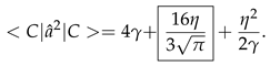
Let us come to the calculation of some mean values taking parameter . The mean value of is
The next quantity is expressed as
3. Evolution in the extended space
Indeed, the etalon picture cannot be applied in the general case to QG because one cannot resolve the constraints. It is believed that the Grassmann variables allow writing a Lagrangian in a form where there are no constraints at all [19,20,36,37].
The discussion could be started in terms of a continual integral. The transition amplitude from to states is written in the form [38]
where is a gauge fixing function (here, the non-canonical gauge fixing [23] is considered).
The action (3) is invariant relatively the infinitesimal gauge transformations:
where is an infinitesimal function of time. If one takes the differential gauge condition , then (21) follows in
and the Faddev-Popov determinant [38] takes the form of . The functional (20) could be rewritten as
where using the Grassmann variables [38] raises the determinant into an exponent. Here a Grassmann number is considered as a complex conjugate to .
Integration over N could be performed explicitly. In a discrete version, where is discretized over the interval , the term with the delta functions has the form
i.e., an initial value of has to equal a final value . For instance, one may take , and, then, the Lagrangian from Eq. (25) becomes
The action (27) is a fixed gauge action with no Hamiltonian constraint, but instead, the ghost (Grassmann) variables arise in (27). The expressions for the momentums of the Grassmann variables are
where, as usual, the left derivative over the Grassmann variables is implied. The Lagrangian (27), rewritten in terms of momentum acquires the form of
Following Vereshkov, Shestakova et al. [19,20], one may consider the Hamiltonian
as describing the quantum evolution of a system.
To quantize the system, the anticommutation relation has to be introduced for the Grassmann variables
In the particular representation , , , , , , the Schrödinger equation reads as
where the operator ordering in the form of the two-dimensional Laplacian has been used. It should be supplemented by the scalar product
where the measure arises due to the hermicity requirement [18,39]. This measure is a consequence of a minisuperspace metric if the Hamiltonian is written in the form of with , . Thus, the measure takes the form [39]. Formal solutions of the equation (32) can be written as
where the functions u and v satisfy the equation
with
Then, the scalar product (33) reduces to
Although the constraint formally disappears from the theory, one may think that the space of solutions of the Wheeler-DeWitt equation (WDW) equation still plays a role [25]. Otherwise, the question of correspondence with the classical theory, where the Hamiltonian constraint holds, arises. We would like to relate the space of the functions, satisfying the Schrödinger equation (32) with the functions satisfying the equation , i.e., the WDW equation. The operator (36) has the Klein-Gordon form. Thus, the Klien-Gordon-type scalar product has to be used. According to this hypothesis, let us represent the functions u, v as
where the operator , or in the representation (14) and
where, as in (15), only a half-space corresponding to the negative frequencies solution of the WDW equation is taken because only in this case the Klein-Gordon product implies a positive definite norm of a state. The operator (see Appendix in [40]) is a necessary attribute of the scalar product for the Klein-Gordon equation to obtain hermicity. It should be noted that, in fact, the function v does not depend on the time because and commutes with . Thus, the time evolution arises only due to function u, or more accurately, due to the presence of the Dirac delta function in ().
Thus scalar product (37) reduces to
The expression for the mean value of an operator has the form:
where u, v are given by (38), () and it is assumed that an operator does not contain the ghost variables , , that is expectable for physical operators. The limit in (42) implies that an evolution begins at , when and tends to .
The evaluation of the mean values is illustrated schematically in Figure 1. Initially, we start with the negative frequency functions , both satisfying . A direct product of these half-spaces is taken. Then function is multiplied by and runs into an extended space, where “evolution” occurs, and, thus, the mean values of the operators could be evaluated.
Both Schrödinger and Heisenberg pictures are possible with this scalar product. For the last, the time-dependent operators have the form
while the functions u and v have to be used without multiplier .
4. Mean values of scale factor degrees
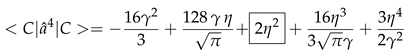
The simplest way to test a theory is to compare it with the etalon picture by calculating the mean value of the squared scale factor, which has to be equal according to (18). To do this by (38), (), (42), it is sufficient to expand in (38) and () and perform the calculation according (42). It turns out to be, that the mean value of actually coincides with that given by (18). The next test is the calculation of . The result of the calculation is
while the etalon model gives another value (19). An origin of this discrepancy could be better seen in the Heisenberg picture. Evolution equations for the Heisenberg operators follows from the operator commutators with the Hamiltonian (36)
It is possible to guess a solution for this particular case:
where . Actually, the calculation of the commutator (45) using (36),(46) gives
which is exactly equal to the derivative of (46) over . Under calculation of the mean value of , third term in (46) does not contribute, and the result coincides with that of the etalon method. However, under the calculation of , the first and third terms in (46) play a role and the discrepancy with the etalon method arises. One could also calculate the mean values of the other degrees of a, which are presented in Table 1. It is interesting to plot these values , that is shown in Figure 2.
5. Discussion and Conclusion
A reasonable expression for the scalar product using the Grassmann variables is suggested. It establishes a relation of a picture with the Grassmann variables to the Klein-Gordon scalar product and allows calculating the mean values of operators in both Schrödinger and Heisenberg pictures, which give the same results. However, it is shown that the mean values of are different for than those calculated in the etalon method, implying an explicit exclusion of the superfluous degrees of freedom. One may guess that the above methods could have different Hilbert spaces. That means that the different wave packets have to be taken for these methods to obtain the same set of operator mean values. Here we cannot find a wave packet , which would give the same mean values as a wave packet for the etalon method.
The possible influence of the Zitterbewegung phenomenon in the extended space was investigated, but without a breakthrough in the results achieved. It should be noted that the quasi-Heisenberg picture corresponds entirely with the etalon method [34,35].
One of the possible ways to correct the picture with the Grassman variables is to assume that the operators of physical observables act not only in k and space, but also in the extended space of the Grassmann variables , . This hypothesis needs further investigation 1 as well the general issue of the scalar product for the approach with the Grassmann variables.
Appendix A. Resolving constraints in the path integral formalism
The theory of constraint systems reduces a system with constraints to the system with the excluded redundant degrees of freedom as proof of formalism [17,18]. Let us consider the action of an arbitrary system with n-dynamical variables q and m constraints
The constraints should be supplemented by additional gauge fixing conditions so that the total system of constraints
leads to a second kind of system with constraints. It is assumed that the determinant , where the Poisson brackets are defined as
Let us consider the transformation to a new set of coordinates
in the transition functional [17,18,20]
where the delta function appears in a second equality after integration over . Last equality has been proved in [18] by taking the functions as the new coordinates , where , or where is associated with momentums , in [17]. As it was shown [17,18], the continual integration could be performed explicitly and only continual integration over coordinates remain in the final result in (A54). However, the result (A54) could be deduced generally. In particular, in the Section 2 we take as the independent variables and exclude using the constraints.
Appendix B. Removing of an “extended Zitterbewegung”
The well-known phenomenon of Zitterbewegung (see [41] and references therein) is an inevitable feature of the Klein-Gordon equation. It arises due to interference of the solutions of the Klein-Gordon equation with the positive and negative frequencies. Here we discuss the solution of the Schrödinger equation (35) with the WDW operator in the right hand side and will consider a possible “extended Zitterbewegung.” In the extended space, the solutions of the Schrödinger equation (35) look as , where the eigenfunctions satisfy
with a different sign of . For the general solution takes the form
where is a Bessel function with a complex index. The solutions for where investigated in [26,27,28,42].
The solution in the extended space is “an heir” of the mass shell solution for a negative frequency (40) by virtue of
where is a Gamma function. The function in () is a superposition of the extended space functions for both and .
Let us take an alternative expression
which consists of the superposition of eigenfunctions with only from
where is a confluent hypergeometric function. It should be noted that the superposition (A11) contains the functions of the extended space corresponding the functions (40) on an on-shell space, but not the functions referring to the positive frequency solutions of the WDW equation.
When tends to zero, the function peaks near , i.e., near . Besides , thus, the limit is an analog of using in () and tending .
Calculations of the mean value of using (A10) gives
As one could see, more complicated regularization is needed, because the limit gives infinity and we need to extract the terms which do not depend on . The situation is similar to that in [34] for this method. After such a regularization, we have the same mean value as in (18). Calculation of gives
 which after regularization, i.e., omitting the terms depending on coincides with (44), but not with the etalon result (18). Thus, removing the possible “extended Zitterbewegung” does not conform to the etalon picture.
References
- Gitman, D.; Tyutin, I.V. Quantization of Fields with Constraints; Springer: Berlin, 1990. [Google Scholar]
- Henneaux, M.; Teitelboim, C. Quantization of gauge systems; Princeton Univ. Press: Princeton, 1992. [Google Scholar]
- Dirac, P. Lectures on Quantum Mechanics; Belfer Graduate School of Science, Yeshiva University: NY, 1967. [Google Scholar]
- Giddings, S. Black hole information, unitarity, and nonlocality. Phys. Rev. D 2006, 74. [Google Scholar] [CrossRef]
- Barvinsky, A.O.; Kamenshchik, A.Y.; Vardanyan, T. Comment about the vanishing of the vacuum energy in the Wess-Zumino model. Phys. Lett. B 2018, 782, 55–60. [Google Scholar] [CrossRef]
- Cherkas, S.L.; Kalashnikov, V.L. An approach to the theory of gravity with an arbitrary reference level of energy density. Proc. Natl. Acad. Sci. Belarus, Ser. Phys.-Math. 2019, arXiv:gr-qc/1609.00811]55, 83. [Google Scholar] [CrossRef]
- Cherkas, S.L.; Kalashnikov, V.L. Eicheons instead of Black holes. Phys. Scr. 2020, 95, 085009. [Google Scholar] [CrossRef]
- Cherkas, S.L.; Kalashnikov, V.L. Vacuum Polarization Instead of “Dark Matter” in a Galaxy. Universe 2022, 8, 456. [Google Scholar] [CrossRef]
- Cherkas, S.L.; Kalashnikov, V.L. Dark Matter in the Milky Way as the F-Type of Vacuum Polarization. Phys. Sci. Forum 2023, 7, 8. [Google Scholar] [CrossRef]
- Carballo-Rubio, R.; Filippo, F.D.; Liberati, S.; Visser, M. Singularity-free gravitational collapse: From regular black holes to horizonless objects, 2023, [arXiv:gr-qc/2302.00028]. arXiv:gr-qc/2302.00028].
- Haridasu, B.S.; Cherkas, S.L.; Kalashnikov, V.L. A reference level of the Universe vacuum energy density and the astrophysical data. Fortschr. Phys. 2020, 68, 2000047–1912. [Google Scholar] [CrossRef]
- Burdík, C̆. ; Navrátil, O. Dirac formulation of free open string. Univ. J. Phys. Appl. 2007, 4, 487–506. [Google Scholar]
- Cherkas, S.L.; Kalashnikov, V.L. Quantum evolution of the universe in the constrained quasi-Heisenberg picture: From quanta to classics? Grav. Cosmol. 2006, 12, 126–129. [Google Scholar]
- Cherkas, S.L.; Kalashnikov, V.L. An inhomogeneous toy model of the quantum gravity with the explicitly evolvable observables. Gen. Rel. Grav. 2012, 44, 3081–3102. [Google Scholar] [CrossRef]
- Cherkas, S.; Kalashnikov, V. Quantization of the inhomogeneous BianchiI model: quasi-Heisenberg picture. Nonlin. Phenom. Complex Syst. 2013, 18, 1–15. [Google Scholar]
- Cherkas, S.; Kalashnikov, V. Quantum Mechanics Allows Setting Initial Conditions at a Cosmological Singularity: Gowdy Model Example. Theor. Phys. 2017, 2, 124–135. [Google Scholar] [CrossRef]
- Faddeev, L.; Popov, V.N. Covariant quantization of the gravitational field. Sov. Phys. Usp. 1974, 16, 777–789. [Google Scholar] [CrossRef]
- Faddeev, L.; Slavnov, A. Gauge Fields. Introduction to quantum theory; Addison-Wesley Publishing: Redwood, CA, 1991. [Google Scholar]
- Savchenko, V.; Shestakova, T.; Vereshkov, G. Quantum geometrodynamics in extended phase space - I. Physical problems of interpretation and mathematical problems of gauge invariance. Grav. Cosmol. 2001, 7, 18–28. [Google Scholar]
- Vereshkov, G.; Marochnik, L. Quantum Gravity in Heisenberg Representation and Self-Consistent Theory of Gravitons in Macroscopic Spacetime. J. Mod. Phys. 2013, 04, 285–297. [Google Scholar] [CrossRef]
- Upadhyay, S. Field-dependent symmetries in Friedmann–Robertson–Walker models. Ann. Phys. 2015, 356, 299–305. [Google Scholar] [CrossRef]
- Chauhan, B. Quantum symmetries and conserved charges of the cosmological Friedmann-Robertson-Walker model. Eur. Phys. Lett. 2022, 140, 40001. [Google Scholar] [CrossRef]
- Ruffini, G. Quantization of simple parametrized systems, 2005, [arXiv:gr-qc/gr-qc/0511088].
- Kleefeld, F. On some meaningful inner product for real Klein—Gordon fields with positive semi-definite norm. Czec. J. Phys. 2006, 56, 999–1006. [Google Scholar] [CrossRef]
- Cianfrani, F.; Montani, G. Dirac prescription from BRST symmetry in FRW space-time. Phys.Rev. D 2013, 87, 084025. [Google Scholar] [CrossRef]
- Gryb, S.; Thébault, K.P.Y. Bouncing unitary cosmology I. Mini-superspace general solution. Class. Quant. Grav. 2019, 36, 035009. [Google Scholar] [CrossRef]
- Gielen, S.; Menéndez-Pidal, L. Singularity resolution depends on the clock. Class. Quant. Grav. 2020, 37, 205018. [Google Scholar] [CrossRef]
- Gielen, S.; Menéndez-Pidal, L. Unitarity, clock dependence and quantum recollapse in quantum cosmology. Class. Quant. Grav. 2022, 39, 075011. [Google Scholar] [CrossRef]
- Garay, L.J.; Halliwell, J.J.; Marugán, G.A.M. Path-integral quantum cosmology: A class of exactly soluble scalar-field minisuperspace models with exponential potentials. Phys. Rev. D 1991, 43, 2572–2589. [Google Scholar] [CrossRef]
- Bojowald, M. Quantum cosmology: a review. Rep. Progr. Phys. 2015, 78, 023901. [Google Scholar] [CrossRef] [PubMed]
- Balcerzak, A.; Lisaj, M. Spinor wave function of the Universe in non-minimally coupled varying constants cosmologies, 2023, [arXiv:gr-qc/2303.13302]. arXiv:gr-qc/2303.13302].
- Lehners, J.L. Review of the No-Boundary Wave Function, 2023, [arXiv:hep-th/2303.08802]. arXiv:hep-th/2303.08802.
- Barvinsky, A.O.; Kamenshchik, A.Y. Selection rules for the Wheeler-DeWitt equation in quantum cosmology. Phys. Rev. D 2014, 89, 043526. [Google Scholar] [CrossRef]
- Cherkas, S.L.; Kalashnikov, V.L. Evidence of time evolution in quantum gravity. Universe 2020, 6, 67. [Google Scholar] [CrossRef]
- Cherkas, S.L.; Kalashnikov, V.L. Illusiveness of the Problem of Time. Nonlin. Phen. Complex Syst. 2021, 24, 192–197. [Google Scholar] [CrossRef]
- Shestakova, T.P.; Simeone, C. The Problem of time and gauge invariance in the quantization of cosmological models. II. Recent developments in the path integral approach. Grav. Cosmol. 2004, 10, 257–268. [Google Scholar]
- Shestakova, T.P. Is the Wheeler-DeWitt equation more fundamental than the Schrödinger equation? Int. J. Mod. Phys. D 2018, 27, 1841004. [Google Scholar] [CrossRef]
- Kaku, M. Introduction to Superstrings; Springer: New York, 2012. [Google Scholar]
- DeWitt, B.S. Dynamical Theory in Curved Spaces I. A Review of the Classical and Quantum Action Principles. Rev. Mod. Phys. 1957, 29, 377–397. [Google Scholar] [CrossRef]
- Mostafazadeh, A. Quantum mechanics of Klein-Gordon-type fields and quantum cosmology. Ann. Phys. (N.Y.) 2004, 309, 1–48. [Google Scholar] [CrossRef]
- Silenko, A.J. Zitterbewegung of Bosons. Phys. Part. Nucl. Lett. 2020, 17, 116–119. [Google Scholar] [CrossRef]
- Menéndez-Pidal, L. 2022; arXiv:gr-qc/2211.09173].
| 1 | In this relation, see [22], where auxiliary pair of the Grassman variables is introduced. |
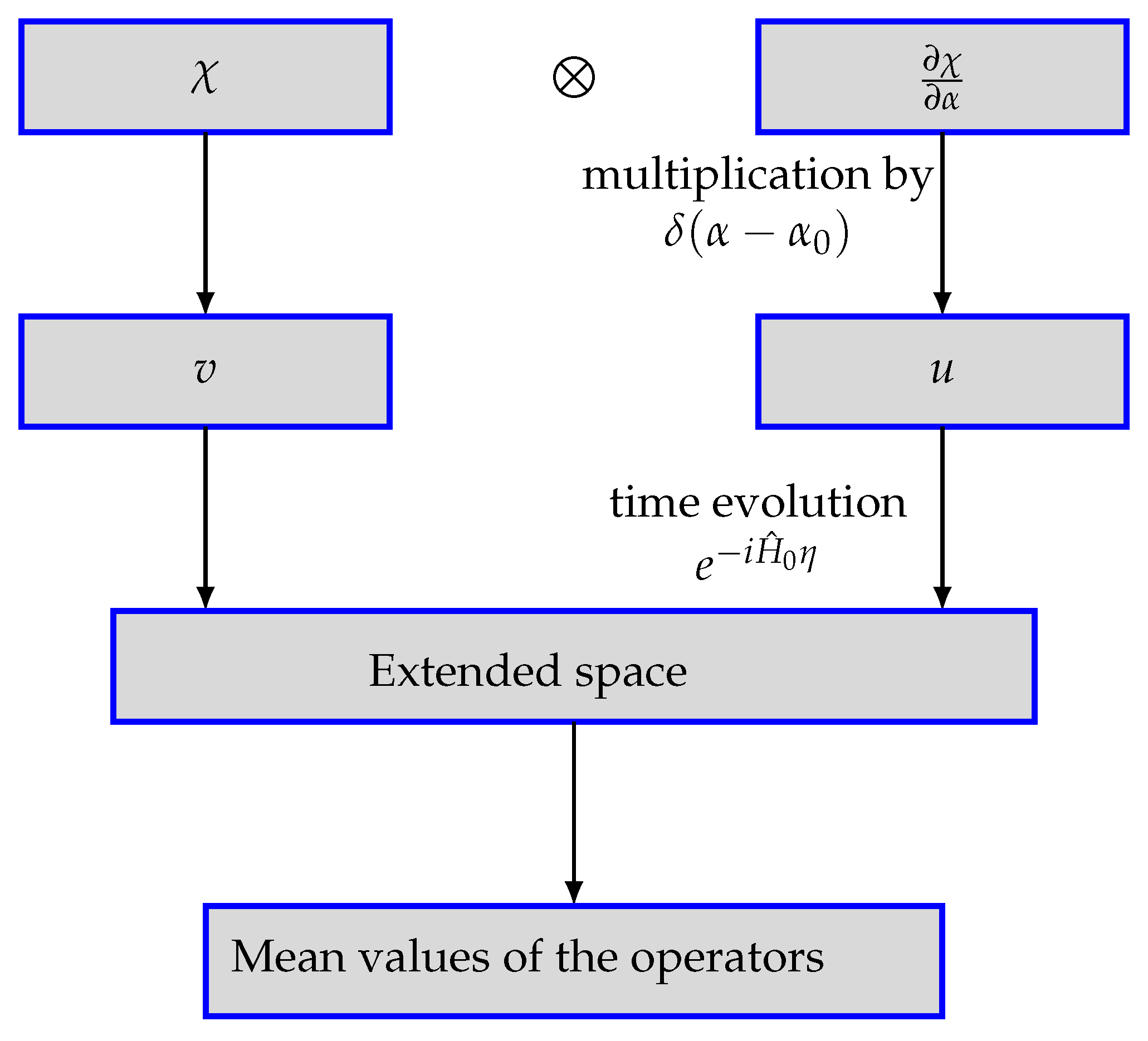
Figure 2.
n-th root of coefficient in the expression for the mean value of th degree of scale factor over wave packet (17). The red and blue curves correspond to the etalon method and that with the Grassmann variables, respectively.
Figure 2.
n-th root of coefficient in the expression for the mean value of th degree of scale factor over wave packet (17). The red and blue curves correspond to the etalon method and that with the Grassmann variables, respectively.
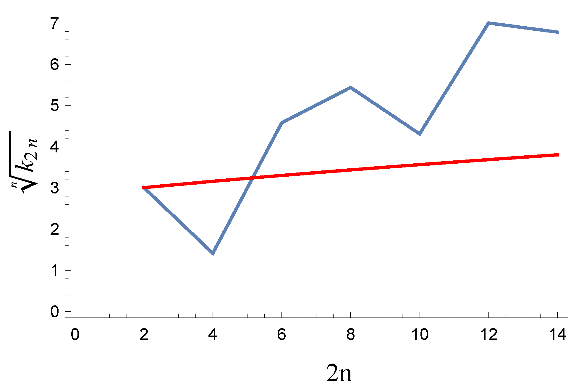

Table 1.
Comparison of the mean values over the wave packet (17).
Table 1.
Comparison of the mean values over the wave packet (17).
| 2 | 4 | 6 | 8 | 10 | 12 | 14 | |
|---|---|---|---|---|---|---|---|
| for the etalon model | |||||||
| for the model with the Grassmann variables |
Disclaimer/Publisher’s Note: The statements, opinions and data contained in all publications are solely those of the individual author(s) and contributor(s) and not of MDPI and/or the editor(s). MDPI and/or the editor(s) disclaim responsibility for any injury to people or property resulting from any ideas, methods, instructions or products referred to in the content. |
© 2023 by the authors. Licensee MDPI, Basel, Switzerland. This article is an open access article distributed under the terms and conditions of the Creative Commons Attribution (CC BY) license (http://creativecommons.org/licenses/by/4.0/).
Copyright: This open access article is published under a Creative Commons CC BY 4.0 license, which permit the free download, distribution, and reuse, provided that the author and preprint are cited in any reuse.


