
Submitted:
15 April 2023
Posted:
17 April 2023
You are already at the latest version
Abstract
The connectivity level of last-generation vehicles is constantly on the rise. The combined use of Vehicle-To-Everything (V2X) connectivity and autonomous driving can provide remarkable benefits through the optimization of the route and speed trajectory. In this framework, this paper focuses on vehicle eco-driving optimization in a connected environment. The virtual test rig of a premium segment passenger car was used for generating the simulation scenarios. The benefits, in terms of energy and time savings, that the introduction of V2X communication, integrated with cloud computing, can have in a real-world scenario were assessed. The Reference Scenario is a pre-defined Real Driving Emissions (RDE) compliant route, while the simulation scenarios were generated by assuming two different penetration levels of V2X technologies. The associated energy minimization problem is formulated and solved by means of a global optimization algorithm, i.e., Dynamic Programming (DP). The optimization framework includes information coming from the surrounding environment, e.g., traffic lights state, speed limits, distance to travel, etc. The simulations show that introducing a smart infrastructure along with optimizing the vehicle speed in a real-world route can potentially reduce the required energy by 54% while shortening the travel time by 38%. Finally, a sensitivity analysis is performed on the bi-objective optimization cost function to find a set of Pareto optimal solutions, between energy and travel time minimization.
Keywords:
Dynamic Programming
; Vehicle-to-Everything
; Real-World Scenario
; Energy Minimization
; Eco-driving
; Speed Optimization
1. Introduction
With climate change threatening the future of our environment and society, implementing immediate and effective strategies to curb Greenhouse Gas (GHG) emissions is the need of the hour. The transportation sector is one of the guiltiest parties, accounting for 35% of the worldwide energy consumption [1]. Road vehicles, especially passenger cars and road freight transport vehicles, account for 86% of the global share [2].
Along with GHG emissions, road congestion is a current problem for transport policy at all levels. According to Joint Research Centre (JRC), the cost of road congestion in Europe is estimated to be over €110 billion a year [3]. Not to mention the dramatic effects that traffic has on the increased air pollution [4] and environmental noise [5]. Despite allowing competing flows of traffic to safely cross busy intersections, traffic signals lead to increased congestion in urban areas.
In this framework, global regulatory targets and customer demand are pushing the automotive industry to develop vehicles with improved fuel economy to curb GHG emissions [6]. On the other hand, integrated with the feasible technical solutions aimed at improving the efficiency of current propulsion systems [7], the adoption of Connected and Automated Vehicles (CAVs) could lead, in the next decade, to a major technological revolution in the mobility sector. The benefits of mass adoption of CAVs can range from enhanced road safety [8], improved traffic handling [9], and reduced fuel consumption [10]. Moreover, creating systems in which information and communication technologies can be easily exchanged, namely Intelligent Transportation Systems (ITS) [11], can also have a beneficial effect on reducing congestion in urban areas. Connected vehicles, featuring Vehicle-to-Vehicle (V2V) and Vehicle-to-Infrastructure (V2I) technologies [12], can have access to the Signal Phase and Timing (SPaT) of traffic lights. This information can be directly transmitted to vehicles through a Dedicated Short Range Communications (DSRC) technology [13] or may become available by the traffic control center through cellular and Wi-Fi networks, namely Cellular Vehicle-to-Everything (C-V2X) [14]. The C-V2X potentiality could be further boosted by a possible coupling with the new 5G mobile network [15] or a joint use of DSRC and C-V2X communications [16]. Alternatively, several studies have demonstrated that SPaT information may be inferred via on-board cameras [16] and via crowdsourcing [17].
Traditional approaches focused more on signal control methods to enhance traffic flow at signalized intersections, such as signal timing optimization [9], or actuated signals application in real-world traffic [18] that could allow to smooth traffic oscillations and decrease vehicle waiting times at intersections. However, with the recent advances in ITS technology, it is also possible to focus on vehicle control, i.e., using V2V and V2I communications to develop eco-driving algorithms. Authors in [19] demonstrated how upcoming traffic signal information can be used by a vehicle’s adaptive cruise control system to reduce idle time at traffic lights and fuel consumption, while [20] introduced a novel software for detecting and predicting the SPaT to enable a Green Light Optimal Speed Advisory (GLOSA) system: i.e., a speed corrector to avoid unnecessary halts at traffic lights. [21] takes into account also the performance degradation of the GLOSA system due to queuing effects and actual tracking driver errors, while [22] introduces the uncertainties of SPaT information due to varying patterns of traffic lights. In the literature, several other applications of eco-driving optimization have been shown: [23] proposes an algorithm to jointly adjust vehicle speeds at intersections and signal timings, while [24] proposes a dynamic eco-driving system for signalized corridors based on an arterial velocity planning algorithm. [24] also assesses the effect of different penetration rates of their algorithm through a sensitivity analysis. Finally, [25] assesses the benefits of incorporating near-term technologies in a predictive management strategy.
From the powertrain control point of view, the increasing adoption of connected vehicles can allow for simultaneously optimizing powertrain control and velocity profile. Several studies have explored methods for optimizing the vehicle velocity profile for Battery Electric Vehicles (BEVs) as well as for Internal Combustion Engine Vehicles (ICEVs). In [26], Dynamic Programming (DP) is used to optimize the velocity of a BEV, while in [27] the fuel consumption reduction of a DP-based algorithm is assessed on a heavy-duty ICEV. However, Hybrid Electric Vehicles (HEVs) and plug-in Hybrid Electric Vehicles (pHEVs) can benefit the most from embedding them in an ITS, since the information from the surrounding environment can be used to optimize their control strategies [28] [29]. Vehicle-to-Everything (V2X) communication along with cloud computing adoption [30] may enable a change of paradigm of the energy management problem: from an instantaneous optimization to globally minimizing it over the entire driver route [31]. In many studies, DP is used for obtaining the optimal solution, but the heavy computation burden of this strategy has made its use largely limited to obtaining an offline performance benchmark. Suitable simplifications to the problem can make the DP real-time implementable, as shown in [32], or the optimization problem can be solved in a remote and/or distributed cloud computing environment [33]. Alternatively, in [34], the optimal solutions provided by DP are used to train Recurrent Neural Networks (RNNs) in improving the energy management of a pHEV.
In this framework, this work aims to assess the benefits that the introduction of V2V and V2I communication, integrated with cloud computing, can have in a real-world route in terms of energy and time savings. The reference scenario is a pre-defined Real Driving Emissions (RDE) compliant route [35], while the simulation scenarios are generated by assuming two different levels of penetration of V2X technologies. DP is used to solve the associated energy minimization problem, where the optimization framework includes information coming from the surrounding environment, e.g., traffic lights state, speed limits, distance to travel, etc. The simulations show that introducing a smart infrastructure along with optimizing the vehicle speed in a real-world urban route can potentially reduce the required energy by 54% while shortening the travel time by 38%. The results of the proposed analysis must be considered as a benchmark since the simulations are carried out for a simplified urban traffic network with vehicles in almost free flow, i.e., no direct constraints related to preceding vehicles. However, it can be conceptually extended to the case of multiple vehicles equipped with the proposed algorithm.
The rest of the paper is organized as follows. In Section 2 the simulation scenarios are introduced along with the description of the virtual test rig used for the simulations. Then, the eco-driving optimization problem is formulated in Section 3. In Section 4, the results of the optimization algorithm are shown in the two different scenarios. In Section 5, conclusions are summarized and further studies are provided.
2. Case Study
2.1. Simulation Scenarios
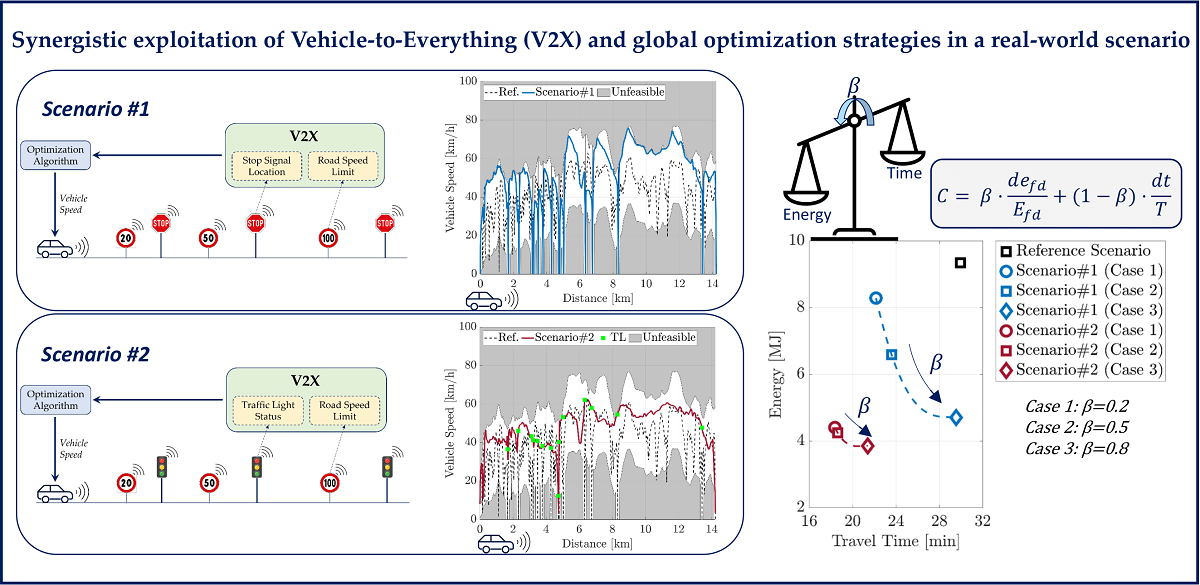
Energy consumption significantly depends on the route characteristics. In this work, in order to fully collect the variability coming from real-world mission profiles, an RDE-compliant route [35] is chosen as a starting point. The RDE driving cycle is considered as the Reference Scenario, without connectivity. As already described, CAVs technology is largely based on the exchange of different types of data between vehicles (V2V) and with the infrastructure (V2I). Two data types may be differentiated: time-invariant and time-variant ones. Time-invariant data, i.e., road network architecture, road elevation, road slope, road speed limits, speed bumps, etc., can be accessed via a Geographic Information System (GIS) server [36]. On the other hand, time-variant data, i.e., traffic information, road closings, SPaT, etc., could be available only thanks to V2X communication. In this study, it is assumed that both time-invariant and time-variant data can be available through cellular/Wi-Fi networks to the vehicle and that the optimization problem can be solved in a cloud domain. In this framework, the optimal velocity profile can be sent to the driver in the vehicle domain. Starting from the RDE route, Scenario #1 and Scenario #2 were created.
2.1.1. Reference Scenario
The Reference Scenario represents a typical real-world mission profile. It is an RDE-compliant route [35] conducted on public roads in the surroundings of the Italian city of Turin. The route, shown in Figure 1, lasted approximately 92 minutes and was 96 kilometers long. The vehicle position was obtained from Portable Emissions Measurement System (PEMS) and combined with a topographic map. In the simulation environment, the speed profile and the vehicle stop of the Reference Scenario are imposed.
2.1.2. Scenario #1
Scenario #1 was designed to assess the benefits that a global optimization can have on the vehicle speed in a real-world mission profile, still respecting all the full stops imposed by traffic and/or infrastructure. It was generated starting from the Reference Scenario and introducing an intersection regulated by a stop sign every time the vehicle comes to a full stop. As detailed in Figure 2, a vehicle speed window was created where the optimizer is allowed to range. The window’s upper and lower boundaries were thought to merge the effects of speed limits and mild traffic conditions in a realistic scenario. Starting from the speed of the Reference Scenario, the upper and lower boundaries are obtained by applying a moving average over a section of 500 meters +- 20 km/h, respectively. It should be noted that the upper boundary never exceeds 135 km/h, and both the upper and lower ones merge to zero whenever a full stop sign is introduced. As depicted in Figure 3, for Scenario #1 it is assumed that the optimizer can have full access to all the time-invariant data and to traffic information.
2.1.3. Scenario #2
Scenario #2 was designed to assess the benefits that the introduction of a smart infrastructure can have on Scenario #1. It was generated starting from Scenario #1 and converting all the stop signs into traffic lights. When designing traffic lights, the quality of the urban realm should be taken into account. According to [37], for urban areas, short cycle lengths of 60–90 seconds are ideal. Moreover, supposing a minor intersection at each traffic light, a 3:2 ratio is suggested for the amount of green time to improve pedestrian compliance and decrease congestion on surrounding streets. Following these guidelines, in this work, the traffic lights were modeled through square waves with a period and a duty cycle of 1 minute and 60%, respectively (the high period corresponds to the green phase). For the sake of simplicity, only red and green phases were considered, while variability was introduced by randomly assigning the initial phase. The speed boundaries coming from Scenario #1 were modified allowing a time-dependent upper boundary in correspondence with the traffic lights, i.e., the upper boundary assumes the moving average value when the traffic light has a green phase. As depicted in Figure 4, it is assumed that SPaT are deterministic and given; thus, the optimizer can have a-priori access to both time-invariant and time-variant data via V2I communication.
2.2. Vehicle Model
The RDE used as the reference scenario was obtained by collecting data from the PEMS mounted on a Mercedes E300de [38]. This vehicle is a state-of-the-art diesel pHEV available in the European market. Figure 5 schematically shows the powertrain layout and Table 1 summarizes the main vehicle and powertrain characteristics. It features a P2 architecture where a Euro 6d-temp 1950 cc diesel engine is integrated into a 90 kW Electric Machine (EM). Both the ICE and the EM are connected, through a Torque Converter and a 9-speed Automatic Transmission, to the rear axle. The vehicle was extensively investigated through an experimental campaign, followed by the validation of a virtual test rig against the experimental data, as explained in [39]. In this work, a simplified version of the vehicle model, relying on a backward kinematic model [40] developed in a MATLAB environment was used. Moreover, since this work presents a powertrain agnostic optimization (i.e., adaptable for each type of vehicle, e.g., ICEV, HEV, pHEV, BEV), the minimization is performed on the energy.
3. Eco-Driving Optimization
In this section, the algorithm for eco-driving is introduced. It takes advantage of V2X communications and is designed for a simplified urban traffic network with vehicles in free flow, i.e., no direct constraints related to preceding vehicles. V2X information can be used to improve the energy efficiency of a vehicle at two different levels:
- Route optimization: choosing the optimal route;
- Eco-driving: optimize the vehicle speed over the defined route.
This work focuses only on the second stage, i.e., eco-driving. The eco-driving problem can be formalized as an optimal control problem, where the optimizer can access both the vehicle’s GPS coordinates (e.g., total trip length, road grade, and speed limits) and V2X information (e.g., SPaT, traffic conditions). Since the position of all the route features varies in a time-based perspective but remains fixed in a distance-based one, it is beneficial to express the model equations in distance-based coordinates: distance (instead of time) becomes the independent variable.
3.1. Optimal Control Problem
In the following, a formulation of the eco-driving problem in distance-based coordinates is proposed:
Where J is the cost function, is the vector of the state variable, is the vector of the control variables, d is the distance variable, is the instantaneous cost function, and is the terminal cost. The cost function is minimized by choosing, in the distance interval the optimal control law that leads to the minimization of the cost function. The cost function defined in Equation (1) is subject to the following constraints:
Where denotes a generic instantaneous constraint, while and are the admissible control and state ranges. Since the main objective of the optimization is to minimize the required energy along with the travel time, the cost function was defined according to the following:
Where and t denote, respectively the energy and time demand at the single distance step, while and T denote, respectively, the energy and time demand along the entire cycle. is a calibration factor that can be used to trade-off between the vehicle energy demand and the traveling time. The constraints for the specific problem concern the physical limitations of the actuators (maximum deliverable power) and of the road infrastructure, e.g., speed limits and traffic lights stop. Moreover, limits regarding the maximum acceleration and deceleration values were imposed to enhance the driver’s comfort in the vehicle. As described in Table 2, in Scenario #1 the vehicle speed is the only state variable and vehicle acceleration is the only control one. As for Scenario #2, since the SPaT is time-dependent, the time must be added as a state variable increasing the computational burden. Dynamic Programming (DP) [41] was used by the Authors to solve the constrained optimal control problem. The open-source MATLAB code developed at ETH-Zurich [42] was used for solving the optimal control problem.
3.2. Variable State Search Grid
DP was first introduced by R. Bellman in 1957 and is based on the concept of breaking up sequential decision problems into a finite number of manageable problems wherein the combination of their solutions leads to the global optimal solution of the entire problem. As already reported in [43], the Achilles heel of discrete DP is the “curse of dimensionality”: in n-dimensional state and m-dimensional control spaces, the number of discrete grid points rises exponentially with the dimensions of n and m [44]. Different techniques could be adopted to reduce the computational time required for finding the most energy-efficient path [45]. In order to reduce the computational time, in this work, a variable state search grid was introduced. As shown in Figure 6, this artifice is particularly relevant for Scenario #2 (two control variables) allowing a reduction in the computational time of more than 95%. The computational times here shown refer to a workstation with the following specifications: Intel(R) Xeon(R) CPU E5-2680 v3 @ 2.50GHz, 64 GB RAM. Figure 7 shows the definition of the variable grid in the urban section. The variable speed grid was defined according to the upper and lower boundaries, supposing that the vehicle can never exceed those limits. The variable time grid was defined allowing the optimizer to sufficiently vary around a predicted time of arrival, where V2X and GPS information plays a key role in providing a time arrival estimation. constraints about the maximum available power are introduced.
4. Results
In this section, the improvements in terms of energy consumption and travel time for Scenario #1 and Scenario #2 are shown. Section 4.1 and Section 4.2 show the results for the case with factor (see 3, i.e., the same weight is given to energy and travel time in the cost function. Section 4.3, instead, shows a sensitivity analysis on the weighting factor . For Scenario #1, the vehicle speed was optimized over the entire selected route in order to assess the performance of the optimization algorithm under different conditions, i.e., urban, rural, and motorway. Instead, since most of the traffic lights are present in the first section of the urban profile the results for Scenario #2 will be shown only for this section. The achievable reduction in terms of time and energy reduction will be shown in the entire driving cycle and only in the selected urban profile for Scenario #1 and Scenario #2, respectively.
4.1. Scenario #1
In this section, the optimization algorithm is applied to Scenario #1. This is aimed at assessing the benefits that optimizing the vehicle speed can have in a real-world mission profile, still respecting all the full stops imposed by traffic or infrastructure. Figure 8 shows the optimized vehicle speed for Scenario #1 (blue line) compared to the Reference Scenario (black dotted line). It seems that the optimizer chooses an almost constant speed only in the rural section. In fact, in the urban and rural sections, the vehicle speed tends to follow as much as possible the lower and upper boundaries, respectively. Figure 9 shows a zoom on the urban section. As expected, Scenario #1 presents smoother accelerations and decelerations if compared to the Reference Scenario, although always respecting the full stops imposed by the infrastructure.
Figure 10 shows the achievable reductions in terms of travel time and energy for Scenario #1 considering the entire route (see Figure 8). Nearly 30% of energy reduction can be obtained while decreasing the travel time by almost 10%. These results are achievable while still respecting all the full stops required by the infrastructure analogously to the Reference Scenario. Note also that regenerative braking is not considered in this analysis, so all the energy required for braking is considered lost.
4.2. Scenario #2
Since the a-priori knowledge of traffic lights SPaT can have major benefits chiefly in an urban environment, the optimization performed by the proposed optimizer will be shown only in these conditions. As already described, Scenario #2 perfectly reproduces Scenario #1 but replaces all the traffic stops with traffic lights. Figure 11 shows the vehicle position as a function of the time axis along with all the traffic light phases. The optimizer chooses the best speed trajectory in order to cross all the intersections at a green light. As evident from Figure 12, since the SPaT of the traffic lights is communicated to the optimizer, the vehicle speed is corrected over the entire route to never cross an intersection at a red light. Differently from Scenario #1 (see Figure 9), where the vehicle speed often laid on the upper boundary when the vehicle was not at an intersection, for Scenario #2 an almost constant speed is preferred. The simulations show that a stop sign (or in general a full stop of the vehicle) is detrimental to both the travel time and the energy required. In fact, the deceleration and acceleration phases preceding and following the full stop of a vehicle cause a major reason for energy loss that should be avoided.
As shown in Figure 13, the introduction of smart infrastructure in the simulated scenario leads to a significant reduction both in terms of travel time and energy. In an urban environment, the energy required by the vehicle can be reduced by half while decreasing the travel time by more than 35%. These findings quantify the maximum achievable reductions in energy and travel time in a framework of connected vehicles able to exploit V2X information in a smart infrastructure.
4.3. Sensitivity Analysis
The sensitivity analysis on the weighting factor was performed to assess the impact that the variation of the relative weights in the cost function can have on the results. In Case 1 () travel time is prioritized at the expense of energy. In Case 2 () the same weight is given to travel time and energy (results shown in Section 4.1 and 4.2). In Case 3 () energy is prioritized at the expense of travel time. Figure 14 shows the Pareto front between energy and travel time for both Scenarios #1 and #2 when varying the value of the weighting factor. Focusing on Scenario #1 (blue marks), for all three cases, the energy consumed to perform the cycle is lower than the Reference Scenario one, mainly due to smoother accelerations and increased cruise traveling time. However, for Case 3 (blue diamond), the excessively conservative driving style, despite decreasing by half the required energy, leads to an increase in travel time if compared to the Reference Scenario. Focusing on Scenario #2 (red marks), Figure 14 reveals that the introduction of a smart infrastructure (such as connected traffic lights) can further improve the trade-off between required energy and total travel time. Moreover, Figure 14 shows that the variation of the weighting factor in Scenario #2 leads to a much more restrained variation in the trade-off energy/time. Prioritizing time does not jeopardize the benefits in terms of energy and vice versa.
5. Conclusions
Over the next decade, Connected and Autonomous Vehicles (CAV) technologies are expected to become ever more commonly available on new vehicles. Although their ultimate goal is to improve safety and convenience for customers, they can provide significant information about the planned driver route and the surrounding environment. The knowledge of this information can improve the energy efficiency of a vehicle while reducing, at the same time, travel time. In this framework, this work assessed the benefits that the introduction of Vehicle-to-Vehicle (V2V) and Vehicle-to-Infrastructure (V2I) communication, integrated with cloud computing, can have in a real-world profile in terms of energy and time savings. The Reference Scenario is a pre-defined Real Driving Emissions (RDE) compliant route, while the simulation scenarios were generated by assuming two different levels of penetration of V2X technologies. The associated energy minimization problem was formulated and solved by means of a global optimization algorithm, i.e., Dynamic Programming (DP). The optimization framework included information coming from the surrounding environment, e.g., traffic lights state, speed limits, distance to travel, etc. Energy reduction benefits are dependent on several factors: route characteristics, traffic conditions, driver behavior, etc. For the route evaluated in this paper, numerical results showed that, in an urban context, introducing a smart infrastructure along with optimizing the vehicle speed in a real-world route can potentially reduce the required energy by 54% while shortening the travel time by 38%. The results of the proposed analysis must be considered as a benchmark since the simulations were carried out for a simplified urban traffic network with vehicles in almost free flow, i.e., no direct constraints related to preceding vehicles. However, it can be conceptually extended to the case of multiple vehicles equipped with the proposed algorithm. Finally, a sensitivity analysis was performed on the bi-objective optimization cost function to find a set of Pareto optimal solutions, between energy and travel time minimization. Future work will be aimed at testing the proposed algorithm on different powertrain topologies (i.e., BEV, ICE, PHEV) and assessing the impact that a real-time traffic simulator can have on the results.
Author Contributions
Conceptualization, L. P., L.T., L.R. and F.M.; methodology, L. P., L.T. and L.R.; software, L. P. and L.T.; writing—original draft preparation, L. P. and L.T.; writing—review and editing, L. R. and F.M.; supervision, L. R. and F.M.; project administration, F.M. All authors have read and agreed to the published version of the manuscript.
Funding
This research was financially supported by Regione Piemonte (Italy) under the Program L.R. 34/04–Programma d’intervento per le attivita produttive 2011/2017–Asse 3 (Internazionalizzazione), Misura 3.1 “Contratto d’insediamento”. Progetto: “Sviluppo di una nuova generazione di sistemi di propulsione di veicoli ibridi ed elettrici”/“Development of a new generation of hybrid and electric propulsion systems”, -Soc. FEV Italia Srl e Politecnico di Torino.
Conflicts of Interest
`The authors declare no conflict of interest.’
Abbreviations
The following abbreviations are used in this manuscript:
| BEV | Battery Electric Vehicles |
| CAV | Connected and Automated Vehicle |
| C-V2X | Cellular Vehicle-to-Everything |
| DP | Dynamic Programming |
| DSRC | Dedicated Short Range Communications |
| EM | Electric Machine |
| GLOSA | Green Light Optimal Speed Advisory |
| GHG | Greenhouse Gas |
| GIS | Geographic Information System |
| HEV | Hybrid Electric Vehicle |
| ICEV | Internal Combustion Engine Vehicle |
| ITS | Intelligent Transportation Systems |
| JRC | Joint Research Centre |
| PEMS | Portable Emissions Measurement System |
| pHEV | plug-in Hybrid Electric Vehicle |
| RDE | Real Driving Emissions |
| RNN | Recurrent Neural Network |
| SPaT | Signal Phase and Timing |
| V2I | Vehicle-to-Infrastructure |
| V2V | Vehicle-to-Vehicle |
| V2X | Vehicle-To-Everything |
References
- IEA. Largest end-uses of energy by sector in selected IEA countries, 2018 – Charts – Data & Statistics. https://www.iea.org/data-and-statistics/charts/largest-end-uses-of-energy-by-sector-in-selected-iea-countries-2018. Accessed: 2022-10-17.
- IEA. Energy consumption in transport in IEA countries. https://www.iea.org/data-and-statistics/charts/energy-consumption-in-transport-in-iea-countries-2018. Accessed: 2022-10-17.
- Christidis, P.; Rivas, N. Measuring road congestion, 2012. EUR 25550 EN. Luxembourg (Luxembourg): Publications Office of the European Union. P: Luxembourg (Luxembourg). [CrossRef]
- Goel, A.; Kumar, P. Characterisation of nanoparticle emissions and exposure at traffic intersections through fast–response mobile and sequential measurements. Atmospheric Environment 2015, 107, 374–390. [Google Scholar] [CrossRef]
- Clark, C.; Paunovic, K. WHO Environmental Noise Guidelines for the European Region: A Systematic Review on Environmental Noise and Cognition. International Journal of Environmental Research and Public Health 2018, 15. [Google Scholar] [CrossRef] [PubMed]
- ICCT. Fit for 55: A review and evaluation of the European Commission proposal for amending the CO2 targets for new cars and vans. https://theicct.org/publications/fit-for-55-review-eu-sept21. Accessed: 2022-10-17.
- Conway, G.; Joshi, A.; Leach, F.; García, A.; Senecal, P.K. A review of current and future powertrain technologies and trends in 2020. Transportation Engineering 2021, 5, 100080. [Google Scholar] [CrossRef]
- Papadoulis, A.; Quddus, M.; Imprialou, M. Evaluating the safety impact of connected and autonomous vehicles on motorways. Accident Analysis & Prevention 2019, 124, 12–22. [Google Scholar] [CrossRef]
- Zhang, L.; Yin, Y.; Chen, S. Robust signal timing optimization with environmental concerns. Transportation Research Part C: Emerging Technologies 2013, 29, 55–71. [Google Scholar] [CrossRef]
- Olin, P.; Aggoune, K.; Tang, L.; Confer, K.; Kirwan, J.; Rajakumar Deshpande, S.; Gupta, S.; Tulpule, P.; Canova, M.; Rizzoni, G. Reducing Fuel Consumption by Using Information from Connected and Automated Vehicle Modules to Optimize Propulsion System Control. SAE Technical Paper 2019-01- 1213, 2019, p 15. [Google Scholar] [CrossRef]
- Commission, E. Directive (EU) 2010/40/EU of the European Parliament and of the Council of 7 July 2010 on the framework for the deployment of Intelligent Transport Systems in the field of road transport and for interfaces with other modes of transport Text with EEA relevance. http://data.europa.eu/eli/dir/2010/40/oj.
- Dey, K.C.; Rayamajhi, A.; Chowdhury, M.; Bhavsar, P.; Martin, J. Vehicle-to-vehicle (V2V) and vehicle-to-infrastructure (V2I) communication in a heterogeneous wireless network – Performance evaluation. Transportation Research Part C: Emerging Technologies 2016, 68, 168–184. [Google Scholar] [CrossRef]
- Zhu, J.; Roy, S. MAC for dedicated short range communications in intelligent transport system. IEEE Communications Magazine 2003, 41, 60–67. [Google Scholar] [CrossRef]
- Dimatteo, S.; Hui, P.; Han, B.; Li, V.O. Cellular Traffic Offloading through WiFi Networks. 2011 IEEE Eighth International Conference on Mobile Ad-Hoc and Sensor Systems, 2011, pp. 192–201. [CrossRef]
- Storck, C.R.; Duarte-Figueiredo, F. A Survey of 5G Technology Evolution, Standards, and Infrastructure Associated With Vehicle-to-Everything Communications by Internet of Vehicles. IEEE Access 2020, 8, 117593–117614. [Google Scholar] [CrossRef]
- Ansari, K. Joint use of DSRC and C-V2X for V2X communications in the 5.9 GHz ITS band. IET Intelligent Transport Systems 2020. [Google Scholar] [CrossRef]
- Fayazi, S.A.; Vahidi, A.; Mahler, G.; Winckler, A. Traffic Signal Phase and Timing Estimation From Low-Frequency Transit Bus Data. IEEE Transactions on Intelligent Transportation Systems 2015, 16, 19–28. [Google Scholar] [CrossRef]
- Hao, P.; Wu, G.; Boriboonsomsin, K.; Barth, M.J. Developing a framework of Eco-Approach and Departure application for actuated signal control. 2015 IEEE Intelligent Vehicles Symposium (IV), 2015, pp. 796–801. [CrossRef]
- Asadi, B.; Vahidi, A. Predictive Cruise Control: Utilizing Upcoming Traffic Signal Information for Improving Fuel Economy and Reducing Trip Time. IEEE Transactions on Control Systems Technology 2011, 19, 707–714. [Google Scholar] [CrossRef]
- Koukoumidis, E.; Peh, L.S.; Martonosi, M.R. SignalGuru: Leveraging Mobile Phones for Collaborative Traffic Signal Schedule Advisory. Proceedings of the 9th International Conference on Mobile Systems, Applications, and Services; Association for Computing Machinery: New York, NY, USA, 2011; pp. 127–140. [Google Scholar] [CrossRef]
- Zhang, Z.; Zou, Y.; Zhang, X.; Zhang, T. Green Light Optimal Speed Advisory System Designed for Electric Vehicles Considering Queuing Effect and Driver’s Speed Tracking Error. IEEE Access 2020, 8, 208796–208808. [Google Scholar] [CrossRef]
- Sun, C.; Guanetti, J.; Borrelli, F.; Moura, S.J. Optimal Eco-Driving Control of Connected and Autonomous Vehicles Through Signalized Intersections. IEEE Internet of Things Journal 2020, 7, 3759–3773. [Google Scholar] [CrossRef]
- Sun, P.; Nam, D.; Jayakrishnan, R.; Jin, W. An eco-driving algorithm based on vehicle to infrastructure (V2I) communications for signalized intersections. Transportation Research Part C: Emerging Technologies 2022, 144, 103876. [Google Scholar] [CrossRef]
- Xia, H.; Boriboonsomsin, K.; Barth, M. Dynamic Eco-Driving for Signalized Arterial Corridors and Its Indirect Network-Wide Energy/Emissions Benefits. Journal of Intelligent Transportation Systems 2013, 17, 31–41. [Google Scholar] [CrossRef]
- Baker, D.; Asher, Z.; Bradley, T. V2V Communication Based Real-World Velocity Predictions for Improved HEV Fuel Economy. SAE Technical Paper 2018-01- 1000, 2018, p 11. [Google Scholar] [CrossRef]
- Lu, D.; Ouyang, M.; Gu, J.; Jianqiu, L. Optimal Velocity Control for a Battery Electric Vehicle Driven by Permanent Magnet Synchronous Motors. Mathematical Problems in Engineering 2014, 2014. [Google Scholar] [CrossRef]
- Hellström, E.; Ivarsson, M.; äslund, J.; Nielsen, L. LOOK-AHEAD CONTROL FOR HEAVY TRUCKS TO MINIMIZE TRIP TIME AND FUEL CONSUMPTION. IFAC Proceedings Volumes 2007, 40, 439–446. [Google Scholar] [CrossRef]
- Zhang, F.; Hu, X.; Langari, R.; Cao, D. Energy management strategies of connected HEVs and PHEVs: Recent progress and outlook. Progress in Energy and Combustion Science 2019, 73, 235–256. [Google Scholar] [CrossRef]
- Pulvirenti, L.; Rolando, L.; Millo, F. Energy management system optimization based on an LSTM deep learning model using vehicle speed prediction. Transportation Engineering 2023, 11, 100160. [Google Scholar] [CrossRef]
- Arthurs, P.; Gillam, L.; Krause, P.; Wang, N.; Halder, K.; Mouzakitis, A. A Taxonomy and Survey of Edge Cloud Computing for Intelligent Transportation Systems and Connected Vehicles. IEEE Transactions on Intelligent Transportation Systems 2022, 23, 6206–6221. [Google Scholar] [CrossRef]
- Gupta, S.; Rajakumar Deshpande, S.; Tufano, D.; Canova, M.; Rizzoni, G.; Aggoune, K.; Olin, P.; Kirwan, J. Estimation of Fuel Economy on Real-World Routes for Next-Generation Connected and Automated Hybrid Powertrains. SAE Technical Paper 2019-01-1213, 2020. [CrossRef]
- Levermore, T.; Sahinkaya, M.N.; Zweiri, Y.; Neaves, B. Real-Time Velocity Optimization to Minimize Energy Use in Passenger Vehicles. Energies 2017, 10. [Google Scholar] [CrossRef]
- Wollaeger, J.; Kumar, S.A.; Onori, S.; Filev, D.; özgüner, ü.; Rizzoni, G.; Di Cairano, S. Cloud-computing based velocity profile generation for minimum fuel consumption: A dynamic programming based solution. 2012 American Control Conference (ACC), 2012, pp. 2108–2113. [CrossRef]
- Millo, F.; Rolando, L.; Tresca, L.; Pulvirenti, L. Development of a neural network-based energy management system for a plug-in hybrid electric vehicle. Transportation Engineering 2023, 11, 100156. [Google Scholar] [CrossRef]
- Commission, E. Commission Regulation (EU) 2017/1151 of 1 June 2017 of the European Parliament and of the Council on type-approval of motor vehicles with respect to emissions from light passenger and commercial vehicles (Euro 5 and Euro 6)... https://tinyurl.com/53ecjp7s.
- Chang, K.T. Geographic information system. International Encyclopedia of Geography: People, the Earth, Environment and Technology: People, the Earth, Environment and Technology 2016, pp. 1–9.
- Sadik-Khan, J. Urban street design guide. New York: NACTO 2012.
- DiPierro, G.; Galvagno, E.; Mari, G.; Millo, F.; Velardocchia, M.; Perazzo, A. A Reverse-Engineering Method for Powertrain Parameters Characterization Applied to a P2 Plug-In Hybrid Electric Vehicle with Automatic Transmission. SAE International Journal of Advances and Current Practices in Mobility 2020, 3, 715–730. [Google Scholar] [CrossRef]
- Millo, F.; Rolando, L.; Pulvirenti, L.; Di Pierro, G. A Methodology for the Reverse Engineering of the Energy Management Strategy of a Plug-In Hybrid Electric Vehicle for Virtual Test Rig Development. SAE International Journal of Electrified Vehicles 2021, 11. [Google Scholar] [CrossRef]
- Millo, F.; Rolando, L.; Andreata, M. Numerical Simulation for Vehicle Powertrain Development. In Numerical Analysis; Awrejcewicz, J., Ed.; IntechOpen: Rijeka, 2011. [Google Scholar] [CrossRef]
- Bertsekas, D. , Dynamic Programming and Optimal Control; Athena Scientific: Belmont, MA, 1995; Volume 1. [Google Scholar]
- Sundstrom, O.; Guzzella, L. A generic dynamic programming Matlab function. 2009 IEEE Control Applications, (CCA) & Intelligent Control, (ISIC), 2009, pp. 1625–1630. [CrossRef]
- Wahl, H.G.; Bauer, K.L.; Gauterin, F.; Holzäpfel, M. A real-time capable enhanced dynamic programming approach for predictive optimal cruise control in hybrid electric vehicles. 16th International IEEE Conference on Intelligent Transportation Systems (ITSC 2013), 2013, pp. 1662–1667. [CrossRef]
- Elbert, P.; Ebbesen, S.; Guzzella, L. Implementation of Dynamic Programming for n-Dimensional Optimal Control Problems With Final State Constraints. IEEE Transactions on Control Systems Technology 2013, 21, 924–931. [Google Scholar] [CrossRef]
- De Nunzio, G.; Canudas de Wit, C.; Moulin, P.; Di Domenico, D. Eco-driving in urban traffic networks using traffic signal information. 52nd IEEE Conference on Decision and Control, 2013, pp. 892–898. [CrossRef]
Short Biography of Authors
 |
Luca Pulvirenti is currently a Ph.D. student in Energetic at Politecnico di Torino, Italy, where he received his Master of Science in Mechanical Engineering in 2019. His research activity is mainly focused on hybrid electric vehicles to assess the emissions reduction that can be achieved by synergically exploiting V2X connections and advanced energy management strategies. From November 1st,2019 to August 31st, 2022, he was a visiting student researcher at Stanford University where he worked on the health estimation of battery packs combining electrochemical modeling and data-inspired algorithms.
 |
Luigi Tresca Luigi Tresca is currently a Ph.D. student in Energetic at Politecnico di Torino in Italy, working in the intelligent mobility field, mainly on research activity based on the integration of artificial intelligence models and vehicle connectivity information into the energy management system of hybrid electric vehicles. He got a MSc in Mechanical Engineering at Politecnico di Torino in 2021 and started his Ph.D. program in November 2022.
 |
Luciano Rolando is an Associate Professor of the Energy Department of Politecnico di Torino where he currently teaches courses on Thermal Machines and Hybrid Propulsion Systems. In 2012, Luciano concluded his Ph.D. in Energetics at Politecnico di Torino defending a thesis on the design of hybrid electric vehicle energy management systems, after which he started a Post-Doc position at the same university. During his post-doctoral research activity, he participated to several projects in collaboration with major OEMs, among which it is worth mentioning the Cayman Project which was entitled by Honda Initiation Grant 2012. In 2017 he was enrolled as an assistant professor through a position funded by Ferrari and, afterwards, he won a tenure track position as Associate Professor. Since 2018 Dr. Rolando has also been an invited lecturer for the IFPEN master program in Powertrain Engineering.
 |
Federico Millo is a full professor of automotive internal combustion engines at Politecnico di Torino, Italy, where he also received his master’s degree in mechanical engineering in 1989, before joining the faculty as a researcher assistant in 1991. His research activity has been entirely focused on internal combustion engines, in particular on the analysis and on the diagnostic of the combustion process, on the use of alternative fuels, on pollutant emissions control in s.i. and diesel engines, on engine modelling and on the development of engine control strategies for conventional as well as for hybrid powertrains. He has been principal investigator for several research projects with major OEMs such as General Motors, Honda and Ferrari and has published over 150 articles based off his research activity. Prof. Millo has been nominated SAE Fellow in 2015, being the first Italian from the Academia to be elevated to the role of Fellow.
Figure 1.
Reference Scenario: vehicle position was obtained from PEMS and combined with a topographic map (Courtesy of Google Maps). The route lasted approximately 92 minutes and was 96 kilometers long.
Figure 1.
Reference Scenario: vehicle position was obtained from PEMS and combined with a topographic map (Courtesy of Google Maps). The route lasted approximately 92 minutes and was 96 kilometers long.
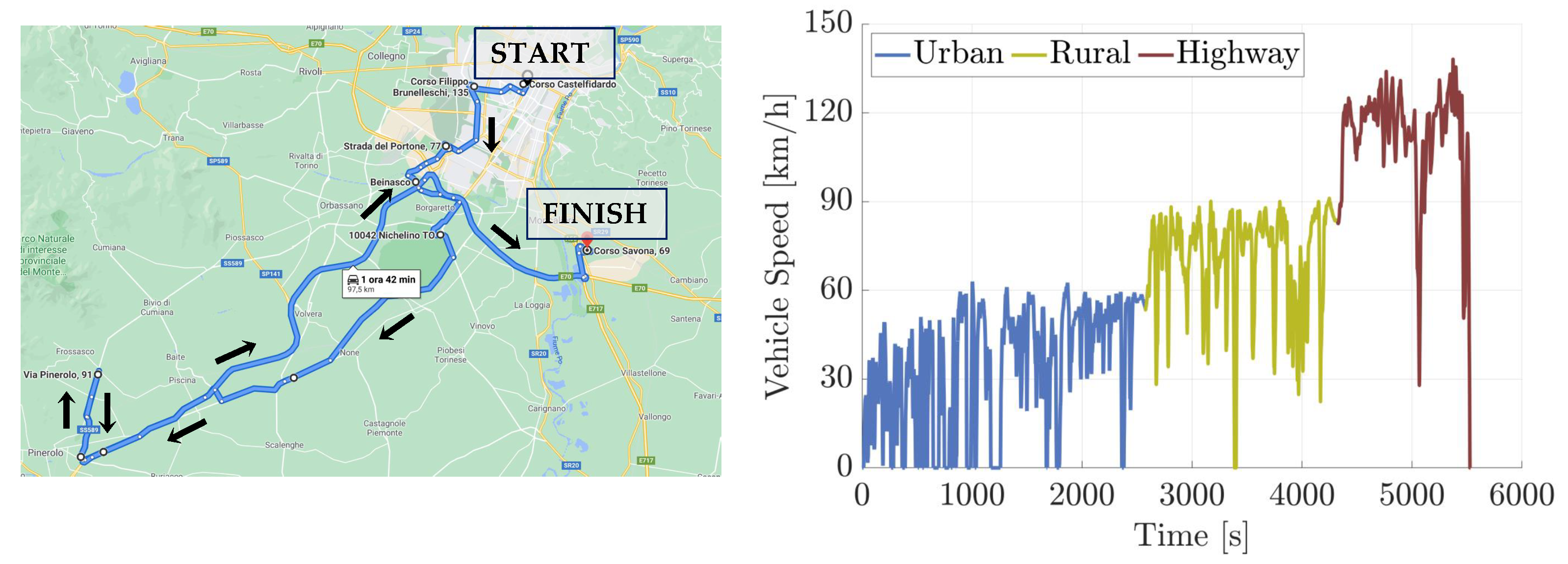
Figure 2.
Speed Boundaries: The upper and lower boundaries of the window were thought to merge the effects of speed limits and mild traffic conditions in a realistic scenario.
Figure 2.
Speed Boundaries: The upper and lower boundaries of the window were thought to merge the effects of speed limits and mild traffic conditions in a realistic scenario.
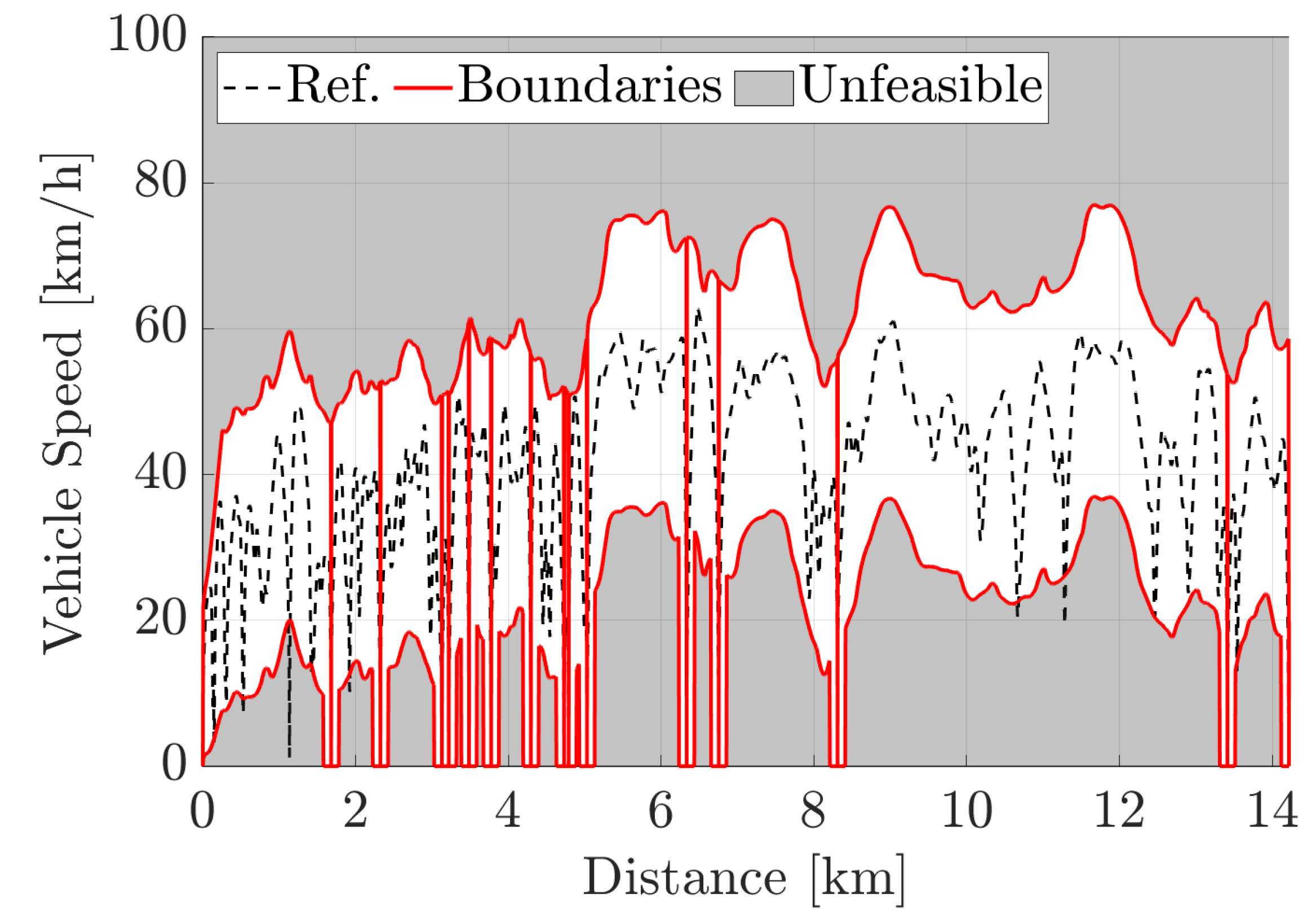
Figure 3.
Scenario #1: it was generated starting from the Reference Scenario and assuming an intersection regulated by a stop sign every time the vehicle comes to a full stop.
Figure 3.
Scenario #1: it was generated starting from the Reference Scenario and assuming an intersection regulated by a stop sign every time the vehicle comes to a full stop.
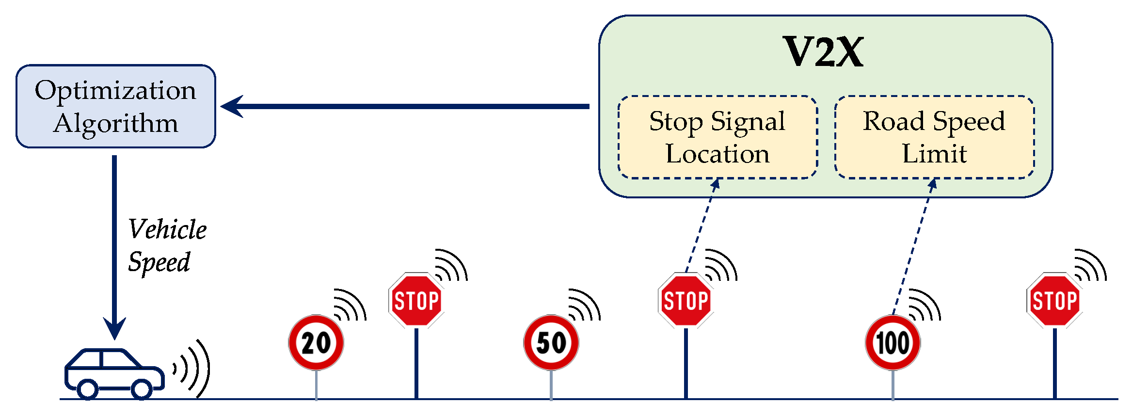
Figure 4.
Scenario #2: it was generated starting from Scenario #1 and converting all the stop signs into traffic lights.
Figure 4.
Scenario #2: it was generated starting from Scenario #1 and converting all the stop signs into traffic lights.
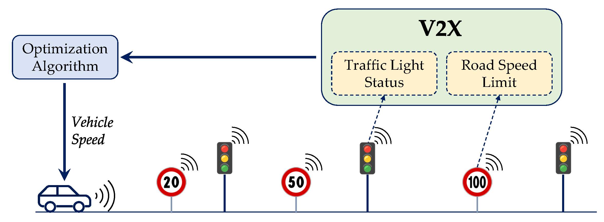
Figure 5.
Powertrain layout: a diesel engine is connected through an auxiliary clutch to an EM. Both the ICE and the EM are connected to the AT by means of a torque converter.
Figure 5.
Powertrain layout: a diesel engine is connected through an auxiliary clutch to an EM. Both the ICE and the EM are connected to the AT by means of a torque converter.
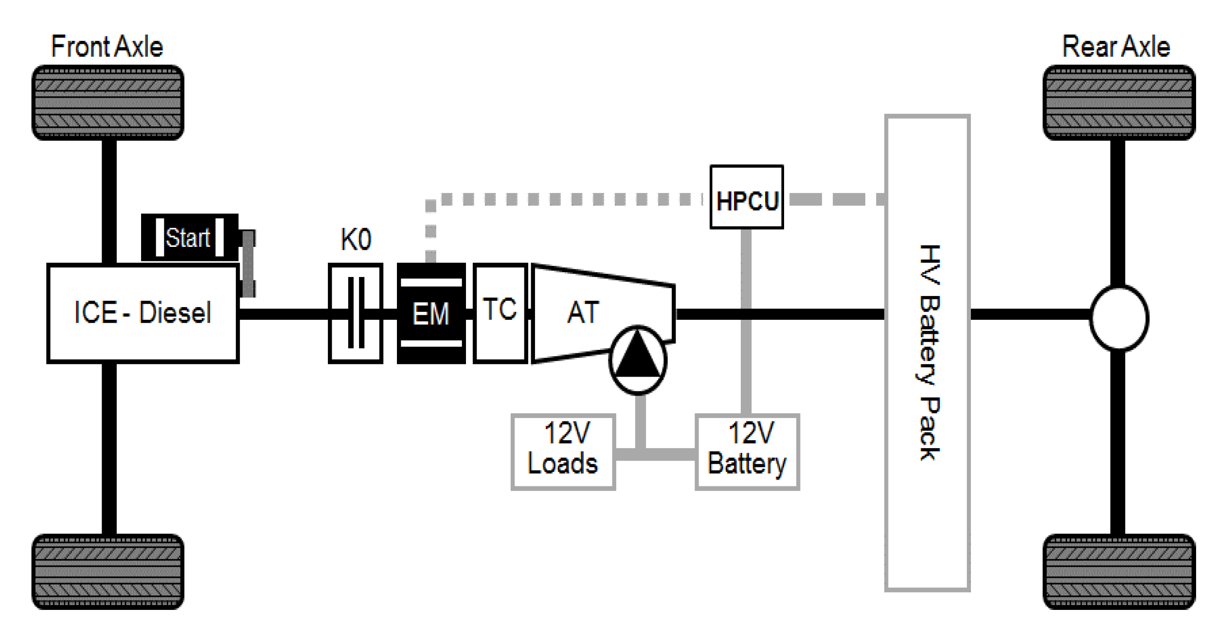
Figure 6.
Scenario #2: computational time for the optimal control problem with a fixed state search grid (grey) and a variable state search grid (light blue). The variable grid allows a reduction in the computational time of more than 95%.
Figure 6.
Scenario #2: computational time for the optimal control problem with a fixed state search grid (grey) and a variable state search grid (light blue). The variable grid allows a reduction in the computational time of more than 95%.
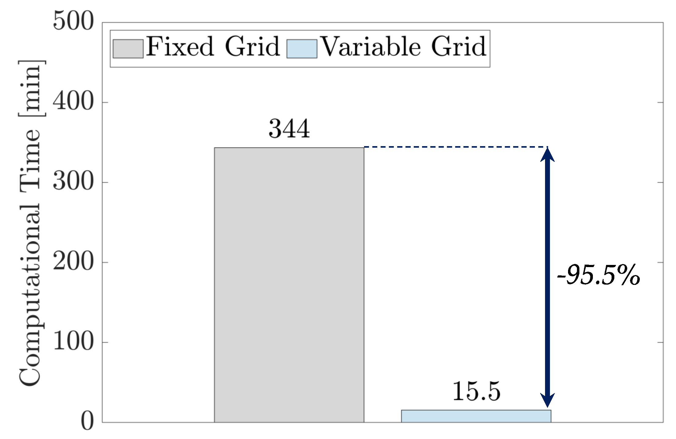
Figure 7.
Variable state search grid: the variable speed grid was defined according to the upper and lower boundaries, supposing that the vehicle can never exceed those limits. The variable time grid was defined allowing the optimizer to sufficiently vary around a predicted time of arrival.
Figure 7.
Variable state search grid: the variable speed grid was defined according to the upper and lower boundaries, supposing that the vehicle can never exceed those limits. The variable time grid was defined allowing the optimizer to sufficiently vary around a predicted time of arrival.
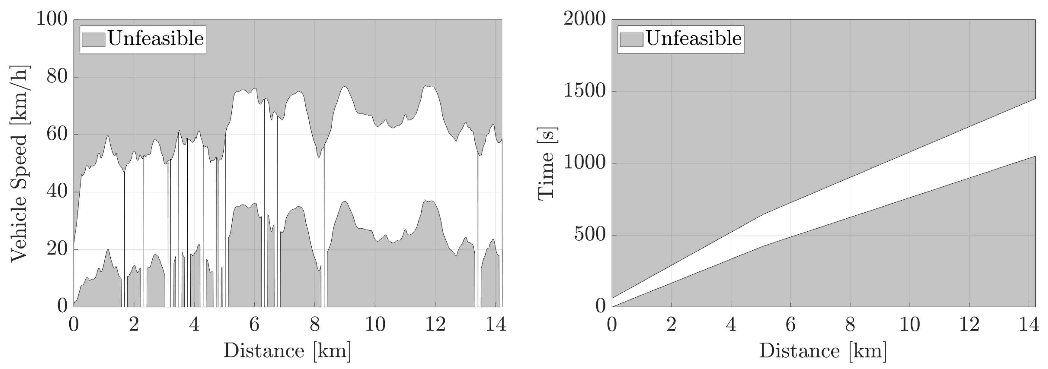
Figure 8.
Scenario #1: optimized vehicle speed compared to the Reference Scenario on the RDE-compliant route.
Figure 8.
Scenario #1: optimized vehicle speed compared to the Reference Scenario on the RDE-compliant route.
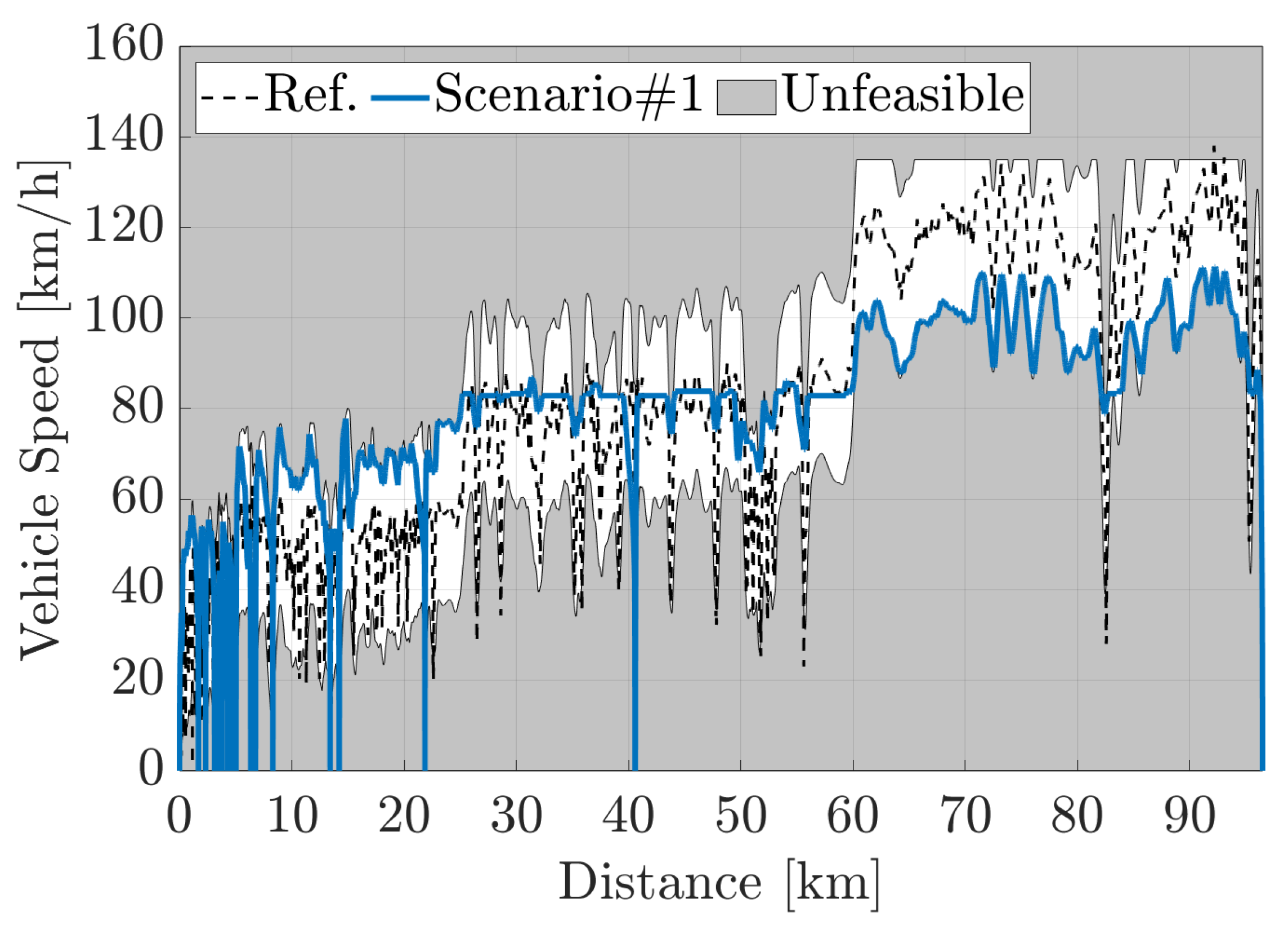
Figure 9.
Scenario #1: optimized vehicle speed compared to the Reference Scenario on the urban section of the RDE-compliant route.
Figure 9.
Scenario #1: optimized vehicle speed compared to the Reference Scenario on the urban section of the RDE-compliant route.
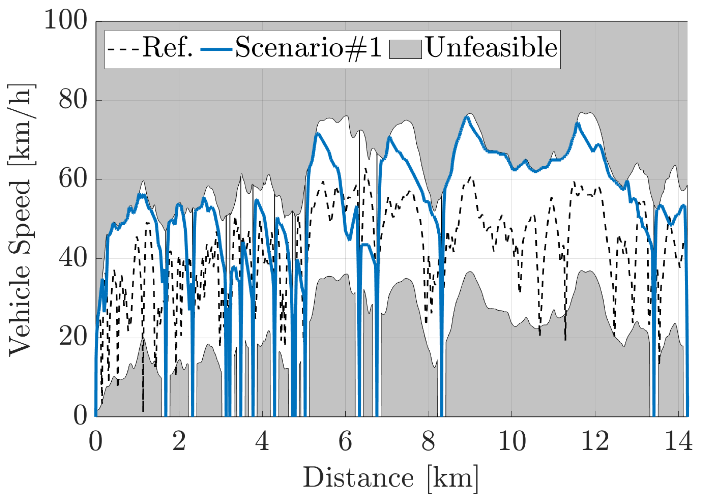
Figure 10.
Scenario #1: achievable reductions in terms of travel time and energy on the RDE-compliant route.
Figure 10.
Scenario #1: achievable reductions in terms of travel time and energy on the RDE-compliant route.
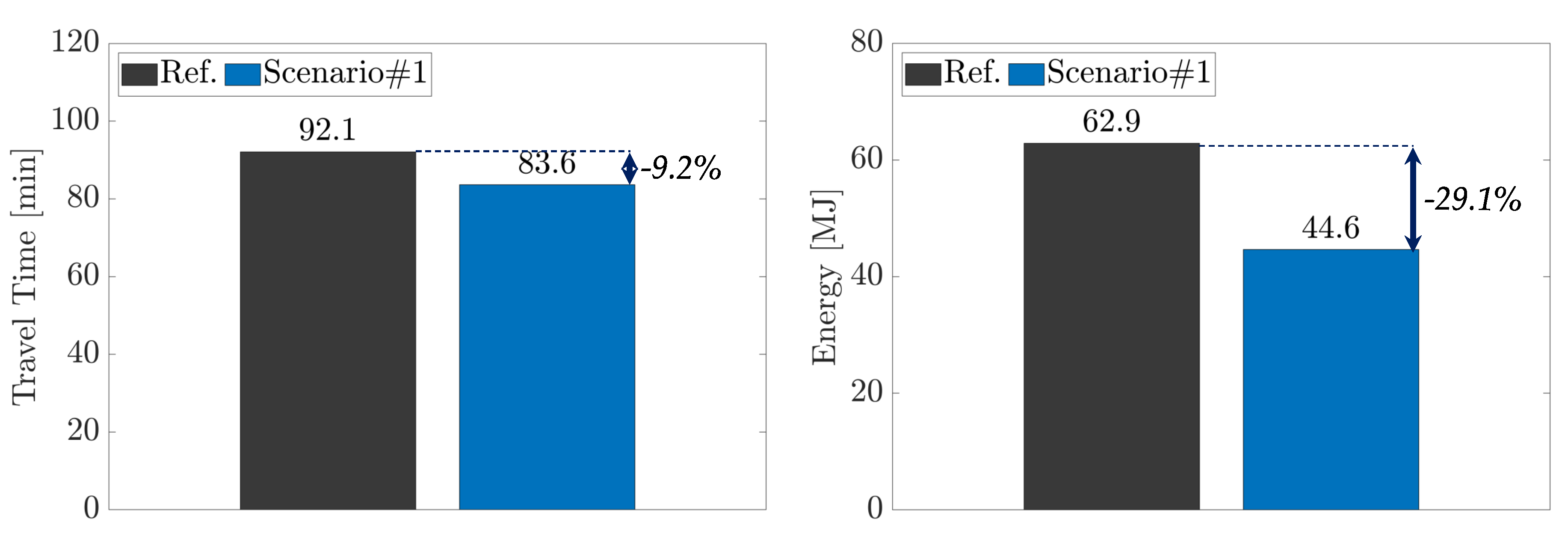
Figure 11.
Scenario #2: vehicle position as a function of the time axis along with all the traffic light phases. The optimizer chooses the best speed trajectory in order to cross all the intersections at a green light.
Figure 11.
Scenario #2: vehicle position as a function of the time axis along with all the traffic light phases. The optimizer chooses the best speed trajectory in order to cross all the intersections at a green light.
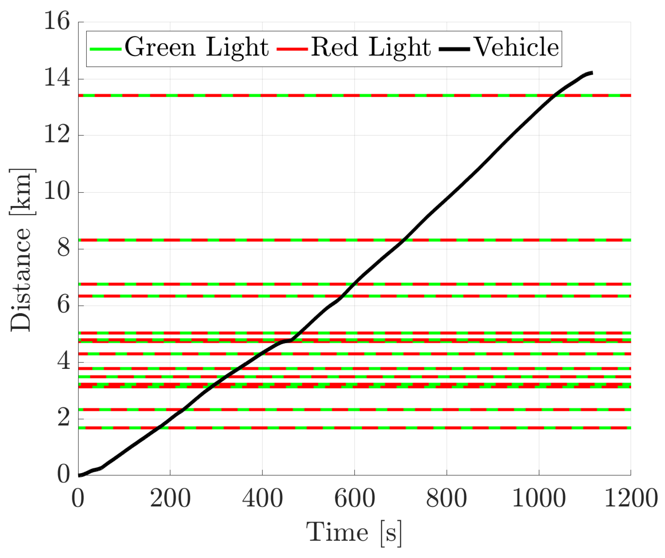
Figure 12.
Scenario #2: optimized vehicle speed compared to the Reference Scenario on the urban section of the RDE-compliant route.
Figure 12.
Scenario #2: optimized vehicle speed compared to the Reference Scenario on the urban section of the RDE-compliant route.
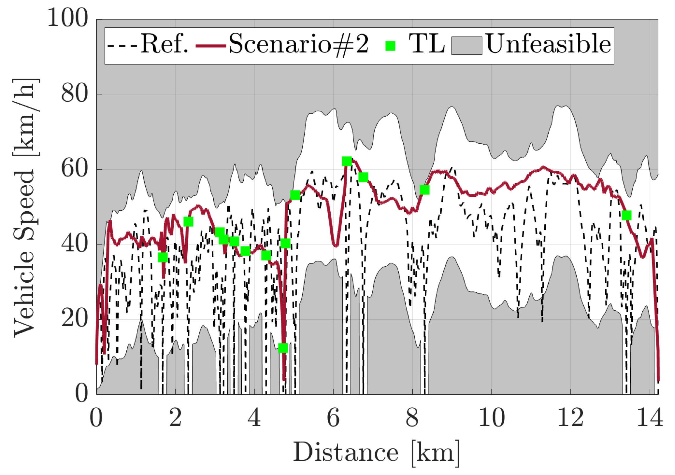
Figure 13.
Scenario #2: achievable reductions in terms of travel time and energy on the urban section of the RDE-compliant route.
Figure 13.
Scenario #2: achievable reductions in terms of travel time and energy on the urban section of the RDE-compliant route.
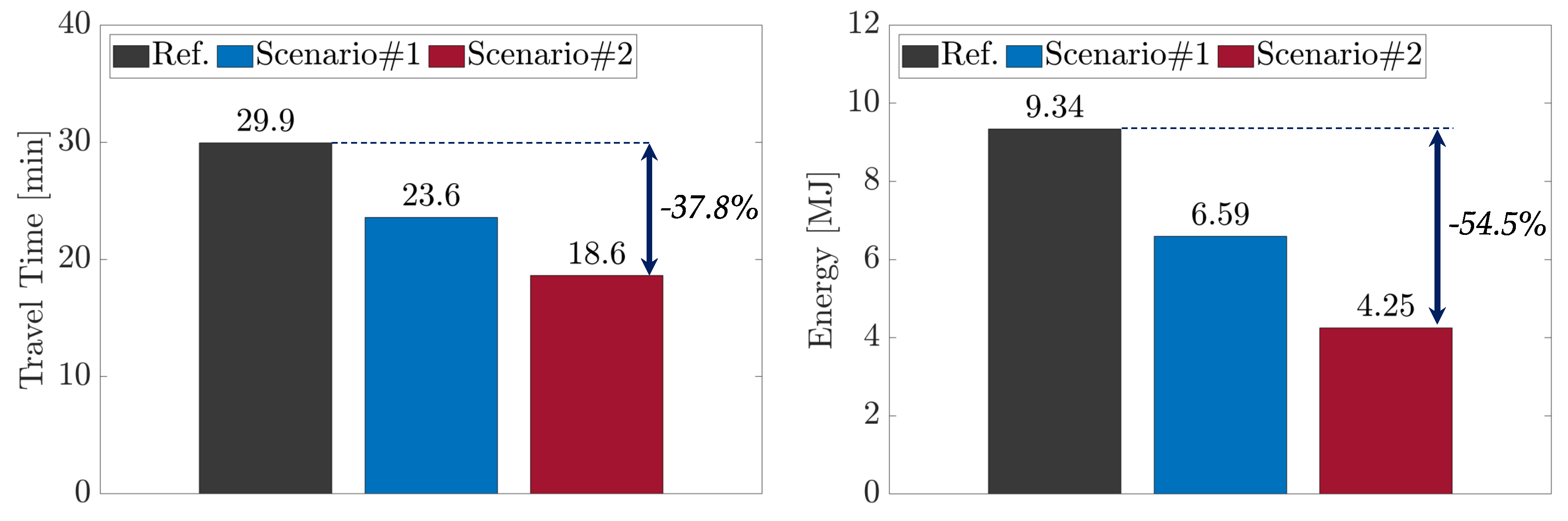
Figure 14.
Pareto front between energy and travel time for both Scenario #1 and Scenario #2 when varying the value of the weighting factor .
Figure 14.
Pareto front between energy and travel time for both Scenario #1 and Scenario #2 when varying the value of the weighting factor .
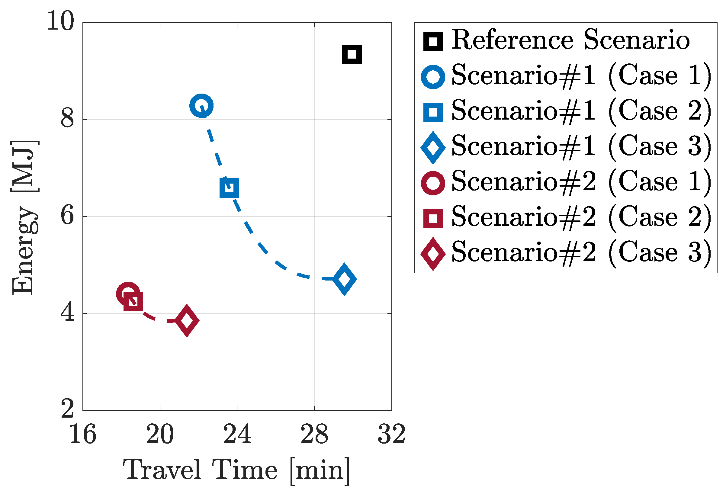

Table 1.
Vehicle and powertrain main specifications.
| Vehicle | Curb Weight [kg] | 2060 |
| Power [kW] @ 100 km/h | 14.9 | |
| Transmission | Type | 9-AT w/ Torque Converter |
| ICE | Type | Turbo Diesel |
| # of Cylinders | 4 | |
| Displacement | 1950 | |
| Max Power [kW] | 143 | |
| Max Torque [Nm] | 400 | |
| Compression Ratio | 15.5:1 | |
| EM | Type | PM Synchronous Motor |
| Max Power [kW] | 90 | |
| Max Torque [Nm] | 440 | |
| Max Speed [rpm] | 6000 |
Table 2.
State and control variables for Scenario #1 and Scenario #2.
| Scenario #1 | Scenario #2 | |
|---|---|---|
| State Variables | Speed | Speed, Time |
| Control Variables | Acceleration | Acceleration |
Disclaimer/Publisher’s Note: The statements, opinions and data contained in all publications are solely those of the individual author(s) and contributor(s) and not of MDPI and/or the editor(s). MDPI and/or the editor(s) disclaim responsibility for any injury to people or property resulting from any ideas, methods, instructions or products referred to in the content. |
© 2023 by the authors. Licensee MDPI, Basel, Switzerland. This article is an open access article distributed under the terms and conditions of the Creative Commons Attribution (CC BY) license (http://creativecommons.org/licenses/by/4.0/).
Copyright: This open access article is published under a Creative Commons CC BY 4.0 license, which permit the free download, distribution, and reuse, provided that the author and preprint are cited in any reuse.


