
Submitted:
16 November 2025
Posted:
18 November 2025
You are already at the latest version
Abstract
We present a geometric field theory in which the action and field equation are constructed from a vector field and its covariant derivative and have full general covariance in a higher-dimensional spacetime. The field equation is the simplest possible generalisation of the Poisson equation for gravity consistent with general covariance and the equivalence principle. It contains the Ricci tensor and metric acting as operators on the vector field. If the symmetrised covariant derivative is diagonalisable across a neighbourhood under real changes of coordinate basis, spacetime coincides with a product manifold. The dimensionalities of the factor spaces are determined by its eigenvalues and hence by its algebraic invariants. Tensors decompose into multiplets which have both Lorentz and internal symmetry indices. The vector field decomposes into conformal Killing vector fields for each of the factor spaces.The field equation has a `classical vacuum' solution which is a Cartesian product of factor spaces. The factor spaces are all Einstein manifolds or two-dimensional Riemannian manifolds. All have a Ricci curvature of roughly the same order of magnitude, or are Ricci-flat. A worked example is provided in six dimensions.Away from this classical vacuum, connection components in appropriate coordinates include $SO(N)$ gauge fields. The Riemann tensor includes their field strength. Unitary gauge symmetries act indirectly on tensor fields and some or all of the unitary gauge fields are found amongst the $SO(N)$ gauge fields. Symmetry restoration occurs at the zero-curvature `decompactification limit', in which all dimensions appear on the same footing.
Keywords:
compactification
; Kaluza-Klein
; unification
; gravity
; gauge fields
; symmetry breaking
; product manifolds
; general relativity
; field equation
; orbits and stabilisers
1. Introduction
1.1. Einstein’s Search for a Unified Field Theory
Following the publication of general relativity (GR) in 1915, Einstein famously spent much of the rest of his life in the search for a unified field theory of gravity and electromagnetism. In the course of this search, he looked into extending the dimensionality of spacetime and also into notions of distant parallelism. From the analysis presented in this paper, it seems clear that he could not have succeeded in his aim, due to a lack of certain conceptual ingredients which were not understood in his lifetime.
Firstly, unification of gravity with non-gravitational forces, in the way that Einstein desired, requires a modern understanding of these forces as gauge fields associated with local symmetries. Two crucial papers in developing this notion were those by Yang and Mills[1] published in the year before Einstein’s death, and Utiyama[2] published in the year after.
Other key ingredients are the transformation properties of coset spaces and the concept of symmetry breaking. These were developed, and the relationships between them revealed, in the 1960s (see Section 2.2). These concepts were not applied to higher-dimensional theories until the late 1970s and early 1980s, and even then, not usually in ways which were consistent with Einstein’s cherished principle of general covariance (see Section 2.1).
These would have been necessary ingredients for Einstein’s approach to be successful. In addition, the concepts underlying the analysis of distant parallelism were usefully developed by Pereira and others in the 2000s and early 2010s – see, for example,[3,4]. This paper and its predecessors[5,6] make use of all of these ingredients to take the subject of Kaluza-Klein theories and spontaneous compactification in a new direction, while staying faithful to the principles and philosophy of Einstein’s search.
1.2. Challenges to Achieving Unification and General Approach of This Paper
The current frontier of our understanding of how our universe works is based on two types of theory.
One is quantum field theory, which describes the working of the strong and electroweak interactions. In this framework, gauge potentials are coupled to matter fields by replacing partial derivatives with covariant derivatives.
The other is GR, describing gravity, which could be termed a ‘geometric field theory’. In GR, there are also covariant derivatives, containing the Levi-Civita connection. This connection transforms in a similar way to gauge potentials. The depth of these parallels was first brought to light by Utiyama[2] in 1955.
In light of this, vast effort has gone into developing a quantum field theory of gravity. The problems with this are well known. Much of the motivation for this has been the success of the quantum field theory framework, both in its predictive power and in unifying interactions. For example, it has allowed us to understand that electromagnetism and the weak interaction are facets of a single electroweak interaction.
GR, however, is a very different type of theory. Its symmetries are not internal symmetries relating components of field multiplets, but the symmetries of four-dimensional spacetime. Moreover, its basic concepts are geometrical ones of connections and curvature, which are not manifest in the quantum field theories.
It seems far from obvious that a unified framework for handling both gravity and other interactions should be based on quantum field theory. It must contain quantum field theories and GR as limiting cases, but why should it not be a geometrical field theory or indeed some other kind of theory, as yet unknown?
Indeed, the first ‘unification theories’ were classical field theories. Maxwell’s electromagnetism unifies magnetic and electrical effects in a single theory. While quantum mechanics was still being developed, Nordström[7,8,9], Kaluza[10] and Klein proposed theories which sought to unify gravity and electromagnetism. These were based on adding an extra spatial dimension to the four-dimensional spacetime of relativity.
Kaluza-Klein theory succeeded in reproducing the Einstein-Hilbert-Maxwell action, although its method for explaining charge quantisation was not consistent with observed masses[11]. Furthermore, after the Second World War, attention turned to the strong and weak nuclear interactions. The quantum field theory framework was found to be admirably suited to describing these. Theories of spontaneous symmetry breaking were developed within this framework. Initially, this work focused on global symmetries, but this was extended to local symmetries[12,13,14,15,16], allowing electromagnetism to be unified with the weak interaction[17,18] and then the strong interaction[19].
A further issue with Kaluza-Klein theory was that it provided no reason for one of the dimensions to be compact. This was addressed when the mechanism of spontaneous compactification was proposed in the late 1970s. The early papers utilised a scalar potential, based on the techniques of spontaneous symmetry breaking[20,21]. By contrast, some papers in the early 1980s triggered compactification using a gauge field[22,23,24].
However, these papers sought to incorporate ‘internal’ interactions, which are described in terms of unitary symmetries. These are not symmetries of spacetime. The geometry to describe the gauge fields for these interactions is one based on fibre bundles. Therefore research focused on mechanisms which would result in these fibre bundle structures after compactification. Furthermore, O’Raifeartaigh’s no-go theorem[25] limited the way in which these symmetries could be unified with those of the Poincaré group. O’Raifeartaigh looked at ways in which the Lie algebras of the Poincaré group and an internal symmetry could be embedded in a larger Lie algebra. He found that ‘none of these (except the direct sum) seems to be particularly attractive from the physical point of view’. This conclusion was strengthened for quantum field theories by the Coleman-Mandula no-go theorem[26]. The only known exception to this was supersymmetry (which in addition provided a solution to the hierarchy problem, by guaranteeing cancellation of quadratic divergences at all orders in perturbation theory). Consequently, most of the research either includes supersymmetry and supergravity explicitly or is constructed in such a way as to facilitate supersymmetric extensions.
We take a different approach in this paper. Unitary groups can be defined in terms of the inner products of complex vectors. Unitary symmetries therefore arise naturally when considering spinor multiplets. They do not appear in the transformation properties of the tensor fields of GR. However, the outer product of a spinor and its conjugate or adjoint can always be decomposed into tensor fields. A unitary group acts on the spinor and its conjugate or adjoint, but this induces a transformation on the tensors of the outer product. These transformations include orthogonal or pseudo-orthogonal transformations, which are isometries on the tangent space, and are amongst the general linear transformations induced by changes of coordinates. We therefore take the approach that a geometric unified field theory should include tensors of orthogonal groups related to internal symmetries.
Unlike the theories based on fibre bundles, we start by asking what spontaneous compactification would look like if the extra dimensions are real spacetime dimensions on exactly the same footing as the four familiar ones. For an N-dimensional theory, bases on a given tangent space are then related by elements of a group isomorphic to . The orthonormality of a frame basis is preserved by a subgroup isomorphic to its maximal pseudo-orthogonal subgroup. This is the group of transformations we want to be included in those of the outer product of the spinor and its conjugate or adjoint.
It is possible to study the decomposition of the group of basis changes with respect to its maximal pseudo-orthogonal subgroup. This leads naturally to the Weitzenböck connection of teleparallelism[5].
However, for the current study, it turns out to be the Levi-Civita connection and the associated covariant derivative of a vector, , which are crucial to the spontaneous compactification described here. This is due to the Levi-Civita connection’s role in describing curvature. (Although it would be interesting to translate the study here into the teleparallel language and see what that reveals.) The field equation we shall derive is based upon this quantity . We will derive it in two different ways. The more comprehensive method is by finding a covariant version of Poisson’s equation for gravity. But prior to that, we shall take a model building-type approach, giving heuristic reasons why we want to use this quantity, constructing an action from it, and finding the corresponding Euler-Lagrange equation.
The primary decomposition of is also different from that in [5] – it is with respect to a direct product of general linear groups[6]. However, one or more of these general linear groups correspond to the compact subspace, and these are then decomposed further, with respect to their maximal orthogonal subgroups. This is what allows the identification of the gauge fields. It is therefore important to understand this kind of decomposition from the outset.
1.3. Structure of This Paper
In Section 2, we summarise some aspects of existing literature in two fields of research:
- Kaluza-Klein theories and spontaneous compactification;
- Non-linear realisations and spontaneous symmetry breaking.
As indicated above, this paper navigates the subtle interplay between the concepts in these two bodies of theory. The existing Kaluza-Klein theories and models of compactification vary widely in their features. The theory presented in this paper has similarities and differences with each of these, so we take time to spell these out. In a similar way, the analysis in this paper includes symmetry breaking, and while the mathematics is very similar to that used in non-linear realisations, the way the symmetry is broken is very different. Also, most theoretical physicists have a superficial knowledge of this subject area at best, so it is worth providing a summary.
Having done this, we are in a position to provide a clearer, more detailed expression of what motivates this study, which we do in Section 3. This culminates in providing a motivation for basing our field equation on and using orbits of its ‘index-aligned’ part to determine the compactification pattern.
From this point, we are able to get into the real substance of this fully covariant model of compactification. But this paper is the third of a series on this subject and some recapping of the content of the other two is necessary, before we can progress to new material. This is done in Section 4. The first part of this recaps relevant parts of [5]: its decomposition of the group of changes of coordinate basis and the two types of connection it describes. The second part summarises [6] and its analysis of Kaluza-Klein-type compactification on a product spacetime. It covers:
- the decomposition with respect to a direct product of general linear groups;
- how the presence of diagonalisable tensors provides information about these groups and the dimensionalities of the factor spaces;
- the decomposition of tensors on these spaces;
- how the Levi-Civita connection for such spaces can describe both gravity and gauge fields.
The detailed new material starts in Section 5. In this short section, we describe how the index-aligned part of , , may be used as the tensor which determines dimensionalities of the factor spaces and symmetries of the compactified spacetime.
While this determines the dimensionalities and symmetries, it does not tell us about the curvature of spacetime and the distribution of the field . For this, we need a field equation. This is the subject of Section 6 and Section 7.
In Section 6, we take a linear sum of two terms as a Lagrangian density. One is a mass term for and the other is the trace of the square of . This gives a second order differential equation. We then rewrite this in a way which involves the Ricci tensor. Thus we determine the field equation up to a proportionality constant.
In Section 7, we take a different approach. We focus on gravity in four-dimensional spacetime, and note that Laplace’s equation for gravity is not generally covariant, being based on scalars and three-vectors. We search for an amended version of it which is both tensorial and consistent with the equivalence principle, by examining the three-acceleration of a test particle freely falling in a gravitational field. The result is an equation in – essentially, a four-dimensional version of that which we had found in Section 6, with the term resulting from the mass term reduced to zero. This allows us to identify the four-dimensional part of the field equation of Section 6 with (a tensorial generalisation of) Poisson’s equation. This gives us a four-dimensional interpretation of the proportionality constant – in just the way it is determined in GR, but with a simpler correspondence between the tensorial and Newtonian equations.
In Section 8, we note that the field equation is an eigenvalue equation which describes the relationship between curvature and matter distribution. There may be spacetimes for which the operator in this equation is trivial. But for other solutions for which is diagonalisable, its invariants may be used to classify the solutions, according to the dimensionalities of the factor spaces, as set out in Section 5. We then search for solutions which represent the ‘classical vacuum’ of the theory, for an arbitrary number of additional dimensions. We find that there is a solution which four-dimensional spacetime is flat and the space of the additional dimensions is curved. There is also a solution for which both of these are curved, but it requires their Ricci scalars to be around the same order of magnitude.
In Section 9, we apply this theory to the case where . We find the characteristic equation for for a classical vacuum solution, and the constraints on its algebraic invariants. The compact factor space here is a two-sphere. We calculate the Levi-Civita components in polar coordinates. By substituting these into the matrix form of in y-coordinates, we find a configuration of that satisfies the constraints. We also use the Levi-Civita components to find the Ricci tensor and show that the configuration of satisfies the field equation. This provides us with a relation between the radius of the two-sphere and the density of the field. The density needs to be extremely high for compactification to sub-nuclear scales.
This concludes the main content of the paper.
In Section 10, we discuss some issues that were not covered in previous sections. These include:
- Fermionic matter and how this affects the geometry;
- A field equation for the gauge fields;
- Transformations which mix Lorentz tensors;
- Translations;
- Isometries of spherical factor spaces;
- Quantum numbers, including charge quantisation;
- How the model evades O’Raifeartaigh’s no-go theorem;
- Symmetry restoration at the decompactification limit;
- The meaning of energy in the model;
- Infinite curvature and dimensional reduction.
Finally, we conclude in Section 11 with a summary of what we have done and recapping some key features of the model.
1.4. Notation and Mathematical Language
This paper follows the language and notation of its predecessors, [5,6]. It is designed to fit a conceptual structure with group theory at its heart. Indices run as follows:
- Greek indices relate to our familiar four-dimensional spacetime and run ;
- Upper-case Latin indices from the end of the alphabet () relate to additional dimensions and run from 5 to N, where N is the total number of space and time dimensions;
- Upper-case Latin indices from the middle of the alphabet () relate to the whole N-dimensional spacetime and run ;
- Lower-case Latin indices from the middle of the alphabet () run , for example for macroscopic spatial dimensions.
Some other aspects of this, which may take some getting used to for researchers who come from different traditions, are as follows:
- We largely avoid the language of fibre bundles, as we are seeking to emphasise firstly how the group transformations are induced by changes of coordinates, and secondly how four-dimensional spacetime and the compact space relating to internal symmetries are two subspaces of a higher-dimensional spacetime that have similar properties within the theory;
- We usually use indices for coordinate bases and frame bases explicitly, rather than using the language of differential forms and exterior derivatives;
- We avoid talking about ‘tetrad fields’ altogether, preferring to talk about transformations between coordinate bases and various frame bases;
- We use the same indices for coordinate bases and frame bases, as frame bases may also be coordinate bases in some situations, and form part of the same carrier space for the transformations;
- The groups involved in this paper are considered to act directly on the bases on tangent spaces. These bases are given the abstract notation and , rather than considering them as differential operators, with the hat representing an orthonormal basis;
- Where we need to specify which coordinate system a set of tensor components relates to, we will do so by putting it in brackets in a superscript or subscript. For example, the components of a vector in a coordinate system will be written ;
- Where we are evaluating a quantity at a given point, we generally state explicitly which point it is evaluated at, to avoid confusion between the value of the quantity and the functional form of that quantity;
- A metric is denoted with a Roman , for example , to distinguish it from the element of the group G (more clearly than just the position of the indices).
2. Existing Literature from Other Authors
2.1. Kaluza-Klein Theories and Spontaneous Compactification
This subsection reviews some of the research which represented significant developments in these subjects. It focuses particularly on three things:
- The spacetime on which the theory is based;
- What the internal transformation group acts upon (where this is stated);
- How its gauge fields appear in the theory.
It concentrates on papers which are particularly relevant to the study in this article. We will see how diverse these papers are, and how their features vary in how natural they appear.
2.1.1. Kaluza-Klein Theories of the 1920s-1960s
Just six years after GR was published, Kaluza[10] proposed what could be called the first geometric unification theory. The theory presented in this paper was largely algebraic. It postulated a five-dimensional metric, then from this it derived a Levi-Civita connection, a Riemann tensor and a geodesic equation. The electromagnetic potential forms four components of the metric. The connection then contains its field strength, .
The paper says little about geometry. However, the state parameters are taken to be independent or largely independent of the fifth coordinate and this is termed the ‘cylinder condition’. In correspondence relating to this paper between Kaluza and Einstein, Einstein said
so clearly this shape of spacetime was assumed by them.The idea of achieving [a unified field theory] by means of a five-dimensional cylinder world never dawned on me[27]
Klein[30] adapted this theory. Klein used a different metric, with the form[31]
where k is a constant. Again, the connection contains . He calculated the Ricci tensor and the Ricci scalar. The five-dimensional Einstein-Hilbert action was found to equal the four-dimensional Einstein-Hilbert-Maxwell action[31].
He assumed the extra dimension to be a physical one. Indeed, as Goenner[27] puts it,
Then, in a follow-up letter[32], he showed that the periodicity of the extra dimension could lead to the quantization of charge – and that this would require its radius to be of the order of m.A main motivation for Klein was to relate the fifth dimension with quantum physics. From a postulated five-dimensional wave equation …and by neglecting the gravitational field, he arrived at the four-dimensional Schrödinger equation after insertion of the quantum mechanical differential operators
The spacetime here thus isometric to . Klein’s metric may be derived from a canonical metric on this space, using a change of variables set out in his first paper, which in our notation may be written[6]
Note the way that appear as coefficients – that is, they are components of the Jacobian matrix for the transformation.
Jordan and Thiry effectively relaxed this isometry condition (see [28,29] – I do not have access to the original works). They generalised the spacetime to one homeomorphic to Klein’s spacetime, by allowing the radius of the compact dimension to vary over four-dimensional spacetime.
In 1953, Pauli extended Klein’s theory to try to account for isospin in mesons, in work which he never published. However, this research is summarised in an article by Straumann[30]. He replaced Klein’s extra dimension by an field space. Once again, the gauge fields appeared as coefficients in the interval, when expressed in the appropriate coordinates. This essentially results in the Yang-Mills gauge theory. This was the year before Yang and Mills submitted their paper for publication[1], in which an gauge group acts on a two-component wavefunction (for example, representing a proton and neutron). In hindsight, Pauli’s model works by taking advantage of the homomorphism between and , as described in Section 7.4 of [6].
The generalisation of Kaluza-Klein theory for an arbitrary non-Abelian gauge group was put forward by Kerner in 1968[31]. This analysis is explicitly carried out in a fibre bundle formulation. The base space is four-dimensional spacetime and the group space provides the fibres. The aim is to produce the same kind of decomposition of the action as Klein achieved. The resulting differential geometry, in terms of how the gauge fields appear, is somewhat mixed up. A starting postulate is that
Consequently, the gauge field appears in the Levi-Civita connection components in both differentiated and undifferentiated factors. This feature persists into the components of the Ricci tensor. After calculating the Ricci scalar and confirming it has the desired form, the paper then studies the resulting geodesic equation.
This has components1 which in our notation would be written . However, use of local geodesic coordinates means that the appear in the metric for these coordinates (as undifferentiated factors):there is a connection in the bundle, given by a Lie algebra valued 1-form A on the bundle manifold.
2.1.2. Spontaneous Compactification
The study of spontaneous compactification in the 1970s and 1980s was started by Cremmer and Scherk[20]. They proposed a model in six dimensions. The fundamental multiplets in this model were the metric field (with Einstein-Hilbert action), the gauge field of an internal symmetry and a Lorentz scalar multiplet which transformed under the action of the defining representation of . The scalar multiplet acted as a Higgs field which could cause two of the dimensions to spontaneously compactify to a two-sphere. Thus in this paper, the gauge field is put in ‘by hand’ at the outset, while the resulting spacetime has a four-dimensional factor and an factor.
This model was generalised by Luciani[21] to one with an arbitrary number of extra dimensions, which started with the metric field, the gauge field of a group K and a Higgs multiplet. The compact space S was now acted on directly by a group G. If , and the symmetry breaking left unbroken, then the gauge fields after compactification could be associated with the Killing vectors of the one-parameter subgroups of G not in H. However, G could alternatively be a non-trivial subgroup of K. In this case, the maximal subgroup of K which commutes with G would also be left unbroken.
A series of papers in the early 1980s by Volkov, Sorokin and Tkach, and one by Randjbar-Daemi and Percacci, considered models with only metric fields and gauge fields –- no scalar fields were required. The gauge field multiplet acts as a matter source for gravity which causes curvature. Symmetric internal spaces, with the form , are found to be solutions to the field equations satisfying the ansatz that the gauge field strength is covariantly constant in all coordinate directions. H is the holonomy group of the internal space[24]. This may be either a simple group or a product of simple groups[32]. It is not necessary for the gauge field triggering the compactification to be one for the whole of G –- the model can start with gauge fields for H only[23] or even an invariant subgroup of H[32]. The field equations have a solution in which the gauge fields are equal to the spin connections associated with the Levi-Civita connection on the internal space[22,33].
These models, with connections related to spin connections and no Higgs-type multiplet, superficially look different from those of Cremmer and Scherk and Luciani. However, it was shown that when the Luciani model with is applied to a case where the internal space is symmetric, it reduces to the connection-based model[33]. This is because the components of the gauge fields of G which are associated with are non-dynamical: they have zero intensity and can be eliminated using a gauge transformation.
2.1.3. Kaluza-Klein Theories of the 1970s and 1980s
These papers investigating mechanisms of spontaneous compactification also formed a basis for the further development of Kaluza-Klein theories. Various authors did not concern themselves with how compactification arose, but focused on the field content arising from it. Scherk and Schwarz[34] and Salam and Strathdee[35] addressed symmetry aspects of the resulting spacetime, starting with the geometrical fields – the vielbein, metric and connection – and then proceeding to other fields that might be in the system. Salam and Strathdee provided important theory on harmonic expansions on an internal quotient space.
Manton[36], on the other hand, considered symmetry breaking patterns for a gauge field for a simple, compact Lie group on . He looked for solutions where the unbroken gauge group is . The four-dimensional effective Lagrangian turned out to be just that for the bosonic part of electroweak theory.
2.2. Non-Linear Realisations and Spontaneous Symmetry Breaking
This subsection summarises the conceptual development of non-linear realisations and their description in terms of coset spaces, and how these relate to spontaneous symmetry breaking (SSB). It focuses on the aspects which are of most relevance to this paper.
Goldstone’s first paper[37] on SSB and Gell-Mann and Lévy’s paper[38] which introduced the non-linear sigma model were both submitted for publication in Nuovo Cimento in 1960. However, these topics were studied in such different ways that it was not proved until after nearly a decade of research that they were two sides of the same coin.
Goldstone’s paper and a follow-up with Salam and Weinberg[39] looked at potentials with degenerate minima constructed out of scalar fields. They found that whenever a Lagrangian has an invariance under a continuous global symmetry group which is not (fully) shared by its vacuum states, there will be spinless fields of zero mass present. These became known as Goldstone bosons.
Gell-Mann and Lévy considered three models relating to pion decays in a system of pions and nucleons. The third of these effectively took a multiplet of four scalar fields and constrained its length, allowing them to eliminate one of the fields from the Lagrangian. This was the first of many papers in the 1960s in which scalars were included non-linearly in the Lagrangian, so that the full symmetries of the system were not explicit. Much of the early work revolved around one particular realisation of a chiral group (for example, [40,41,42,43]). However, in 1969, Callan, Coleman, Wess and Zumino[44,45] showed how a coset decomposition of a linear Lie group G could be used to find the most general form of a Lagrangian in which a subgroup H was linearly represented but the rest of the symmetries were realised non-linearly.
The geometry of these non-linear realisations was examined further by Isham [46], who introduced the concepts of Killing vectors and of a metric (prompted by Meetz[47]), and later by Boulware and Brown [48].
The extension of Goldstone’s mechanism of SSB to a gauge symmetry became known as the Higgs mechanism, following a series of papers in the mid 1960s[12,13,14], but the non-Abelian case was addressed by Kibble[15]. This paper again used a coset decomposition of the invariance group of the Lagrangian. It pointed out that the vacuum manifold could be identified with the coset space.
This led researchers to realise that non-linear realisations represented the low-energy effective theory where a global symmetry was spontaneously broken - this was shown by Honerkamp [49] in a specific case and by Salam and Strathdee[16] in the general case.
From this viewpoint, the coset space represents the vacuum manifold – a submanifold of the field space of the linear representation which is used to break the symmetry. It is therefore crucial to start with scalar fields in the appropriate representation to allow this. This issue was emphasised by Isham[50]. Once this is done, representatives of can be used to map every other G-multiplet in the system into an H-multiplet.
3. Motivations Behind This Model of Covariant Compactification
3.1. The Geometrised Universe
In 1876, Clifford suggested that the
This idea is expressed by Davies as…variation of the curvature of space is what really happens in that phenomenon we call the motion of matter…That in the physical world nothing else takes place but this variation.[51]
We are familiar with taking measurements in space using a ruler and in time by using a clock. This is the spacetime of the ‘physical world’, as Clifford puts it. It is hard to see how a ruler or a clock could (hypothetically) be applied to the internal field spaces of Gell-Mann and Levy’s sigma models or those in the models proposed by Kerner and Luciani.the forces and fields … themselves being explained in terms of geometry[52].
The idea behind the model proposed here is to see how far we can take Clifford’s notion. There should be a limit which we can smoothly approach in which all the dimensions appear in the equations on an equal footing. That is, the theory should be fully covariant over all N dimensions. In this limit, one cannot distinguish between any of the spatial dimensions. Time would only differ from these by its signature and the consequences of that, as happens in relativity.
However, under conditions which represent the universe we live in, the additional dimensions would form a compact subspace. In this curved spacetime, we would want some components of the curvature to represent gravity and other components to represent gauge fields. That is, the gauge fields would not have to be ‘inserted by hand’ as they are in the papers on spontaneous compactification described above – rather, they would appear in the geometry, as in the original models of Kaluza and Klein.
3.2. The Relation Between Unitary Transformations on Spinors and Orthogonal Transformations on Tensors
The immediate problem is that the known gauge symmetries are unitary symmetries, rather than spacetime symmetries. But a clue to resolving this can be found by considering the symmetries of the compact spaces in the pre-1960 Kaluza-Klein theories described above. In Kaluza and Klein’s work, and its extension by Jordan and Thiry, which includes a gauge field, the compact space is . Rotations around this space form the group . In Pauli’s model, which includes a gauge field, the compact space is . Rotations around this space form the group . These are possible because the unitary group has a vector representation which is an group.
This property is unique to and . However, there is a generalisation which can be used for any unitary group of the form or where , with n an integer.
In this case, the direct action of the unitary group is on a d-dimensional spinor multiplet of an orthogonal group. This spinor transforms as the (direct sum) Weyl representation of , the sole spinor representation of and as a fundamental representation of . For example, if , the group acts directly on a 16-dimensional spinor. This spinor transforms as the direct sum of the two spinors of ; alternatively, it can be seen as the spinor representation of , or as either the left-handed or right-handed spinor of .
The unitary group then acts by conjugation on the direct product of a spinor and its conjugate. This direct product can be decomposed into tensors of the corresponding orthogonal symmetries. preserves orthonormality on complex vector space, which describes the local values of the spinor fields, just as preserves orthonormality on a real vector space, which describes the local values of vector fields contained in the decomposition. The rotations are contained in the indirect action of the unitary group on the outer product.
Hence if we extend our four-dimensional spacetime to include , or additional dimensions, rotations in these extra dimensions may be induced by an transformation of a spinor. The gauge fields of then span part or all of the space of the gauge fields.
The extra dimensions would form a compact space in our universe. This would give the full N-dimensional spacetime an symmetry.
However, we could consider what happens as the curvature of the compact space is reduced steadily to zero. This would give us a ‘decompactification limit’. In this limit, the symmetry would be extended to an symmetry of rotations and boosts.
In such a limit, any matter fields would form multiplets of this full N-dimensional symmetry group. If we want to derive field equations for the model from an action, the action would need to be expressed in terms of these N-dimensional multiplets.
However, in our universe, we expect these to break into multiplets of .
For example, if the universe has two additional dimensions, the decompactification limit is a six-dimensional flat spacetime. Rotations and boosts in this universe form an group. The spacetime has six-dimensional vectors and a rank-two tensor field has two indices running . Under conditions which represent our universe, spacetime becomes a product manifold with two factors: one is our familiar four-dimensional spacetime and the other is a compact two-space. A six-vector then decomposes into a Lorentz four-vector and a two-vector of the internal symmetry. A rank-two tensor will similarly decompose into tensors with Lorentz and internal indices: .
3.3. Symmetry Breaking
This decomposition of tensors of a group into those of a subgroup tells us that the coset space methods of Callan, Coleman, Wess and Zumino[44,45] are the appropriate ones to use. Effectively, the higher-dimensional symmetry is being ‘broken’ into the symmetry of the space with the compact factor. But the way this symmetry is broken is very from that described in Section 2.2. As Salam and Strathdee describe[16], spontaneous symmetry breaking of an internal symmetry occurs when observation energy is reduced below a threshold. In covariant compactification, by contrast, symmetry breaking occurs when curvature is increased above zero. That is, if you reduce curvature to zero, there is no longer anything marking out certain dimensions as special, and they all appear on the same footing. In place of the redefinition of the fields using the coset space representative that Salam and Strathdee describe, we simply have a change of coordinates. One consequence of this is that there are no Goldstone bosons or massive vector fields resulting from covariant compactification. (See Section 4.2.3.)
Now in SSB, the symmetry breaking pattern is determined by algebraic invariants of the Lorentz scalar multiplet which triggers the breaking. For example, if the multiplet transforms as the defining representation of an orthogonal group , the vacuum manifold might consist of all states which satisfy . All of these states have an invariance group of , so this is the subgroup which is realised linearly. (That is, all other fields will be representations of this subgroup at low energies.)
The question for covariant compactification is how the symmetry breaking pattern would be determined. We start by noting that in SSB, is a non-trivial multiplet of the unbroken symmetry group, . We might therefore expect our model to involve a non-trivial multiplet of .
While this is indeed correct, we are in fact breaking more than the symmetry. As explained in [5] and Section 4.1, the set of all changes of basis on a N-dimensional tangent space form a group under the operation of matrix multiplication. The group of changes of basis which preserves orthonormality is a subgroup of this, and is a subgroup within that. The N-dimensional metric has independent components, which depend solely upon the parameters of the corresponding coset space. The Levi-Civita connection and Riemann and Ricci tensors therefore depend upon these parameters and their derivatives.
We are therefore looking to break a group of symmetries down to its subgroup. Now has degrees of freedom; so does a generic rank-two tensor . We are also looking for a tensor which carries information about the curvature of the compactified space. Both of these criteria are satisfied by the covariant derivative of a vector :
– it has degrees of freedom and contains information about the curvature through the connection . This will be the key quantity we work with in developing a fully covariant model of compactification.
4. Relevant Content from My Previous Papers
[5] explains the geometric meaning of the general linear and special orthogonal groups and their relation to two types of connection. [6] describes product spacetimes and the groups of changes of basis on these. It explains how the presence of diagonalisable tensors provides information about these groups and the dimensionalities of the factor spaces. It shows how tensors decompose on these spaces. And it explains how the Levi-Civita connection for such spaces can describe both gravity and gauge fields and gives examples of how these gauge fields can also gauge symmetries. We recap the relevant content from [5] and summarise the main findings of [6] in this section.
4.1. Basis Transformations and Connections
Take a curved pseudo-Riemannian manifold with t time dimensions and s space dimensions. A change of coordinates induces a change of basis at a point A:
Note that is a matrix of values. Carrying out two successive changes of coordinates results in two such matrices, multiplied together. The set of all possible Jacobian matrices at A forms a group which is isomorphic to .
If we choose a pseudo-orthonormal basis on this tangent space, any other pseudo-orthonormal basis is related to it by
where i is an element of a group which is isomorphic to .
Then if we denote the transformation between the chosen frame basis and a chosen coordinate basis by j:
this can be uniquely decomposed into an element of and a representative of the coset space which has no dependence on the group parameters of :
Now if we consider a bundle of tangent spaces across a coordinate neighbourhood, we can choose a field of pseudo-orthonormal frames across this neighbourhood, . Similarly, we have a field of coordinate bases, . These are related by
Given the pseudo-orthonormality of the frame field and the fact that preserves pseudo-orthonormality, the metric then takes the form
If we so choose, we can use the frame field to define a parallelism across the neighbourhood. Then determines the corresponding Weitzenböck connection:
Alternatively, we can use the metric to define the Levi-Civita connection:
There are similarities and differences between the properties of these connections, as shown in Table 1.
For any connection , we may define the covariant derivative of a vector, with components
The Levi-Civita connection determines geodesics, through the geodesic equation:
Its field strength is the Riemann tensor, which describes the intrinsic curvature of :
If a body is in free fall, it is taken to follow a geodesic, as in GR. It is possible to construct a set of coordinates – Riemann normal coordinates – for which the coordinate basis is pseudo-orthonormal along the geodesic. If we wish, we can align the timelike vector in this basis with the four-velocity vector of the body. Then the coordinates constitute a rest frame for the body.
If we take as the rest frame coordinates and as the corresponding basis along the geodesic, this basis is related to that for any set of curvilinear coordinates on by
At a given point A on the geodesic, this is evaluated as
The pseudo-orthonormality of the basis along the geodesic means that the Levi-Civita connection reduces to zero along this curve. But in a curved spacetime, it is not possible for the coordinate basis to be pseudo-orthonormal away from the geodesic. This means that intrinsic curvature may be distinguished by the variation in the Levi-Civita connection with separation from the geodesic. This will be important to us later in this paper.
4.2. Compactification on Product Manifolds
4.2.1. Product Manifolds
[6] looks at Kaluza-Klein theories and compactification on product manifolds. The definition adopted for a generic product manifold is simply that, in the appropriate coordinates, the metric takes a block diagonal form:
Such spaces are not unusual. Most spacetimes of interest in general relativity are products of four one-dimensional spaces – that is, they are completely diagonalisable. A notable exception is the Kerr metric, but even this can take block diagonal form.
Indeed, a two-dimensional cylinder is a product manifold, with factor spaces and . Even the humble two-dimensional plane fits this description, with two factor spaces. Other than these, a simple example was given in [6] of deforming a cylinder to introduce bulges and/or constrictions – resulting in a tube of varying radius – see Figure 1.
Replacing the factor space here with four-dimensional Minkowski spacetime gives us the background spacetime of the Jordan-Thiry model.
The simplest product manifolds are ones in which one or more of the factor spaces are Ricci-flat or are Einstein manifolds. Einstein manifolds (along with all two-dimensional manifolds) have the property that the mixed form of their Ricci tensor is diagonal, with all eigenvalues equal:
These are important to understanding the ‘classical vacuum’ of Kaluza-Klein theories, as described below in Section 4.2.4.
4.2.2. Orbits of Rank-Two Tensors and Diagonalisability
The important insight which underlies much of the analysis in [6] is that under a change of coordinates, the action of on a rank-two tensor in mixed form is a similarity transformation:
Similarity transformations preserve eigenvalues. The eigenvalues of a matrix are completely determined by its ‘algebraic invariants’ – the traces of its powers:
The action of partitions the space of all rank-two tensors into orbits, where every element of an orbit has the same eigenvalues. Some orbits contain diagonal matrices, but some do not. For a start, a diagonal matrix has the property
We write such a tensor and refer to it as ‘index-aligned’. (It is the mixed form of a symmetric tensor, but may not be a symmetric matrix due to the signature of the spacetime.) This property is preserved under the action of . So for a tensor to be diagonalisable under , it must be index-aligned.
However, from any rank-two tensor, we can always construct an index-aligned tensor. This is because an arbitrary rank-two tensor can be decomposed into symmetric and anti-symmetric parts. In their mixed form, these take the forms:
Index-alignment is a necessary but not sufficient condition for a real tensor to be diagonalisable under . Some real, index-aligned tensor matrices have complex eigenvalues – that is, they diagonalise to a complex matrix. This cannot be achieved by the action of , which only contains real matrices. If, instead, a matrix has only real eigenvalues but some of them are repeated, it may or may not be diagonalisable under . Indeed, two matrices can have the same eigenvalues and one is diagonalisable while the other is not. But if matrix has distinct real eigenvalues, it is always diagonalisable under .
4.2.3. Stabiliser Groups and the Product Space Decomposition Theorem
It turns out that the presence of diagonalisable tensors tells us a lot about the group theory and geometry of spacetime. The multiplicities of the eigenvalues of any such tensor determine the ‘breaking pattern’, i.e. which symmetries are realised linearly or ‘unbroken’.
For example, if can be diagonalised to the form
it is invariant under a group which is isomorphic to . These invariance groups, which contain the Lorentz group and an SO(2) group, are valid in any coordinate system, up to equivalence.
Furthermore, any changes of basis in the first four dimensions and/or in the last two dimensions preserve this form for . It is only transformations which mix the coordinates on the two subspaces which result in a non-diagonal form for .
The group G stabilising the diagonal tensor X is a subgroup of J, which provides a new decomposition of :
where is an element of , and L is a representative of which has no dependence on the parameters of G.
can be a direct product of general linear groups. The relationship between J and its subgroups in the case where it is not a direct product is shown in Figure 2.
In Section 6 of [6] it is shown that if L can be consistently defined across a coordinate neighbourhood, then it can be used to define a coordinate basis which can only exist on a product space. Then in Section 12, this is all put together into the following theorem:
Theorem 1.
If any real tensor field of the form can be diagonalised across a region of spacetime with the same multiplicities of its eigenvalues, then
- The spacetime coincides with a product manifold across that region;
- The dimensionalities of its factor spaces are equal to the multiplicities of the eigenvalues;
- The tensor is stabilised by G across the region, where G is a direct product of the general linear groups of basis changes on the factor spaces;
- A representative of the coset space will take us from a generic coordinate basis to a basis relating to a set of coordinates which respect the factor spaces;
- In any coordinate system which respects the factor spaces, the tensor field is diagonalised.
By ‘a coordinate system which respects the factor spaces’ we mean a set of coordinates of which subsets parametrise each of the factor spaces individually: .
So for example, if can be diagonalised across a region to the form (24), the spacetime is a product of a four-dimensional space and a two-dimensional space. Note that a and b do not need the same values everywhere, they just need the same multiplicities. By allowing them to vary, we are promoting them to scalar fields.
Note also that plays a similar role to the one it plays in SSB, except that in SSB, the parameters in its exponent are realised as Goldstone bosons.
4.2.4. Applying the Product Space Decomposition Theorem in the Kaluza-Klein Framework
Given how common product spaces are, the product space decomposition theorem may not seem too impressive. But it has highly significant consequences in the context of Kaluza-Klein theories. In this context, G describes the symmetries of the system which are manifest in the compactified spacetime. On product manifolds, we can decompose tensors in terms of the factor spaces. For example, for the six-dimensional spacetime we have just considered, a six-component vector breaks into a Lorentz four-vector and a two-component multiplet .
Similarly, the Levi-Civita connection components can be assembled into subsets:
The components and vanish if is independent of the coordinates on the compact factor space – a generalisation of Kaluza’s ‘cylinder condition’.
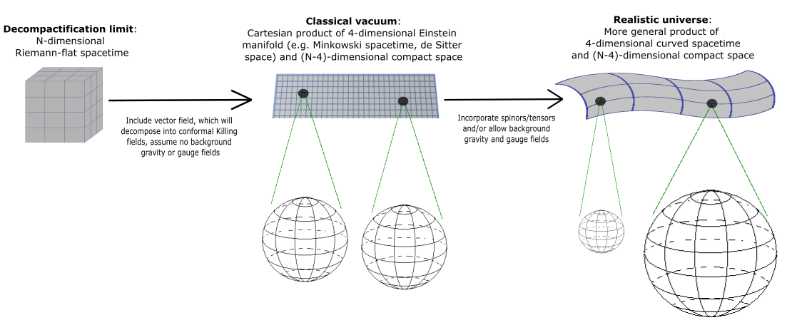
In [6], we ended up with the following interpretation of this framework. In deep space, in the absence of background fields or any passing gravitational waves or waves of the gauge fields, spacetime is represented by a Cartesian (direct) product of four-dimensional Minkowski space and an Einstein manifold or two-dimensional manifold (or a set of these). In the present paper, we generalise this slightly to include cases where the four-dimensional spacetime is an Einstein manifold, such as a de Sitter space. (We look at such solutions of the field equation in Section 8.4.) This Cartesian product is described as the ‘classical vacuum’ of the theory. In y-coordinates (those that respect the factor spaces), the metric has the form
(If is a direct product group, there is more than one factor space and is itself block diagonal.) Meanwhile, the operator (mixed) form of the Ricci tensor is
where is the Ricci scalar of the compact factor space.
When there is gravitating matter or a background gravitational field, these generalise to
and
Adopting more a general coordinate system, where one or more coordinates is a function of both and , gives values to components of the Levi-Civita connections with both types of index. These represent ‘fictitious’ gauge fields - that is, ones with zero field strength.
To get gauge fields with a non-zero field strength, we need to move away from a Cartesian product space, to one where the curvature of the additional dimensions varies with .
Even in two dimensions, we can see how allowing the curvature to vary in this way gives values to the relevant components of the connection. For a tube of varying radius with coordinates , the metric is (see Section 5 of [6]):
So, as we move along x, we find that the radius shrinks or grows, resulting in a change in metric for the space parametrised by , giving us
If the generalised cylinder condition holds – that is, as we move around the compact subspace, the metric for the four-space does not change – the covariant derivative of with respect to four-dimensional spacetime is then
– just as we get in GR – while the covariant derivative of with respect to four-dimensional spacetime is
where
If we now transform to a set of Riemann normal coordinates on the compact factor space (but retain curvilinear coordinates on the four-dimensional spacetime) then these connection components are transformed into a spin connection for . They can be identified with gauge fields of and span part or all of the space of the gauge fields of the corresponding unitary symmetry.
[6] provides two examples of this. In the first, there are two extra dimensions, so we get gauge fields. The vector (defining) representation of is the doublet representation of . can be rewritten as the covariant derivative of a complex scalar. This gives it exactly the right form for the coupling of this field to a gauge field, where that gauge field is proportional to that of .
In the second example, there are three extra dimensions, giving us gauge fields. The vector representation of is the triplet (vector, adjoint) representation of . The gauge fields are proportional to the triplet of gauge fields and couples to them as a vector of .
The field strength tensor for gauge fields, , can be found in the Riemann tensor components for these coordinates. It does not contribute to the Ricci tensors for either factor space. Meanwhile, still describes our normal gravity operating in four spacetime dimensions – it is not diluted by propagating through extra dimensions, as is sometimes claimed of Kaluza-Klein theories.
If one wants to use the language of fibre bundles to describe the product spacetime, this is possible. The oriented orthonormal frames in the tangent spaces for the compact space form a bundle over the four-dimensional spacetime, with structure group . However, this description misses out most of the beauty of this model – in particular, the way that all the factor spaces, compact and non-compact, are treated on the same footing.
5. Using a Covariant Derivative to Determine the Factor Spaces and Symmetry Groups
We decided at the end of Section 3 that the appropriate quantity for breaking J-symmetry is the covariant derivative of a vector. From Section 4.1, we can see that the connection which most naturally describes curvature is the Levi-Civita connection. We therefore utilise the Levi-Civita covariant derivative:
We shall write the matrix of components as for short.
We can now apply the analysis of Section 4.2 to this. The action of J on partitions the space of all possible values of this matrix into orbits. These orbits are characterised by the scalar invariants
If we take the index-aligned part of this tensor matrix,
it has orbits which contain diagonal matrices. By imposing constraints on using its algebraic invariants, we can therefore specify spacetimes which coincide over finite regions with a product space, for which the factor spaces have particular dimensionalities. Away from their classical vacuums, these will have gauge fields amongst the connection components. For example, if diagonalises to (24), we have a four-space on which
and a 2-space, on which
It is worth noting that the trace of is zero. Thus only contributes to the first scalar invariant, . In any coordinate system, this is simply the sum of the eigenvalues of . For example, if diagonalises to (24),
If we calculate this invariant for each factor space, we have
Thus (39) and (40) may be written
and
These are conformal Killing equations, so is a conformal Killing vector for the four-space and is a conformal Killing vector for the compact space. (That is, they generate conformal maps on the manifold.)
6. Deriving a Field Equation from a Lagrangian
The last section explained how the covariant derivative of a vector could be used to fix the dimensionalities of the factor spaces of a product manifold. This leads to a particular decomposition of tensors.
What it does not tell us about is the curvature of the factor spaces. Now, in GR, the field equation determines the curvature of spacetime and the matter distribution. We want a field equation which does likewise for this theory.
There are two approaches to this. The first we shall take is to to construct a Lagrangian from scalar invariants and use the principle of least action. Taken alone, this looks rather like guesswork. But we will see in Section 7 that the same field equation results from the simplest possible generalisation of Poisson’s equation for gravity.
For , the second algebraic invariant looks like a kinetic term:
But we want the extra dimensions to be tightly compact, so we need a mass term:
We therefore take our Lagrangian to be
where k is a constant (dimensionful, but invariant and constant across spacetime). The action integral uses the measure :
where has the property
We then subject to an active variation over the region – one in which the coordinate basis is preserved – which vanishes at the boundary. The field equation then follows by using established procedures. (The method may be found on p146–147 of D’Inverno[53]. It includes making use of the fact that for a contravariant vector density of weight +1, the covariant derivative is equal to the partial derivative).
We thus arrive at the field equation
This does not look much like the field equation of GR. However, by using the relation
we get the following form for the field equation:
where is the Ricci tensor.
In the next section, we derive this equation in four dimensions by generalising Poisson’s equation for gravity. This gives us a value for the proportionality constant, and an interpretation for it in four-dimensional gravitational theory.
7. Deriving a Field Equation by Generalising Poisson’s Equation
7.1. Generalising Laplace’s Equation
We start by considering a test particle – one whose own gravitational field is negligible – moving in a background gravitational field. Newtonian gravitation has a scalar potential, . This means that the work done in moving the particle from one point to another is independent of path; around a closed loop it is zero. Denoting the particle’s Newtonian velocity vector , the acceleration due to the field is
Laplace’s equation for gravity simply equates the divergence of this to zero:
In general relativity, if a test particle has no non-gravitational forces acting on it, it is considered to be in ‘free fall’. For a particle with finite real mass, it moves on a timelike geodesic. Its relativistic velocity vector, whose components we shall denote , is covariantly constant along the geodesic. Hence the free fall acceleration is entirely due to the variation in the transformation between the coordinate basis and the particle’s rest frame along the path.
The result of parallel transporting the velocity vector from one point to another depends on the path taken, and parallel transporting it around a closed loop of intersecting geodesics induces a transformation. We therefore do not expect our generalisation of Laplace’s equation to contain the derivative of a scalar potential.
Now from (17), at any point A on the geodesic,
and
We now define a ‘Newtonian coordinate system’ as one for which
at every point on the geodesic, where is a very small parameter. That is, the change of coordinates may mix up the spatial basis vectors to any extent, but the mixing of the spatial and timelike bases is very limited and . Then using the usual transformation law for vectors together with (55), we have
Substituting these into (54), we find
Thus the spatial components of the acceleration are given by
where c is the speed of light.
Components of the Levi-Civita connection therefore play the role of in (52). Our equivalent of Laplace’s equation (53) should thus involve derivatives of this connection. Given that we noted in Section 4.1 that intrinsic curvature may be distinguished by the variation in the Levi-Civita connection with separation from the geodesic, equation (61) is looking promising. However, this cannot function as a generalisation of the gradient of the gravitational potential , as it is not tensorial. It has been derived from the expression on the right hand side of (54). Taking that expression, , as our ‘potential gradient’ would represent a minor improvement over the right hand side of (61), as it at least has covariance in its indices. But it still will not suffice, for two reasons: it is still not tensorial and furthermore it contains a local vector, , which is only defined on the particle’s path.
We can tackle the second of these issues by replacing the local vector in this expression with the vector field which determines the overall shape of the spacetime, . This gives us . Then finally, to ensure that our ‘potential gradient’ transforms as a tensor, we add on a term. The term we must add is none other than the partial derivative of , giving us back the familiar covariant derivative:
This is the simplest possible generalisation of consistent with general covariance and the equivalence principle.
7.2. Using Poisson’s Equation to Interpret the Proportionality Constant
The relationship between (65) and (49) is obvious: with and , (49) reduces to (65). Now Laplace’s equation is the zero density limit of Poisson’s equation. In Newtonian gravity, it is mass density that is the source of gravity. Similarly, in GR, energy-momentum density is the source of curvature. This suggests that (49) itself might be a covariant generalisation of Poisson’s equation, with k playing the role of density – which seems very plausible given that it is the coefficient of the mass term in (46).
However, there are also indications that mass and density are intrinsically four-dimensional quantities. Perhaps the most stark of these is that the rest mass of a particle is proportional to the norm of its four-momentum. And more pertinently to our study, gravity is curvature in the first four dimensions. This curvature should be related to a four-dimensional energy-momentum density, .
So rather than work with the full N-dimensional equation (49), we will consider it in four dimensions and compare it with Poisson’s equation. Consider the component:
In a coordinate system which becomes Newtonian at A, defining t by
we get
The first term on the left is our generalisation of derived in the previous subsection - this can be expanded to give
where is related by (61) to the three-acceleration caused by . The meaning of the next term is unclear, but it may be that it vanishes in the non-relativistic limit (unless there is a very rapid variation in ) due to the factor of . Assuming this to be the case, comparing with Poisson’s equation for gravity, we then expect the right hand side to reduce to where is the density of the field . If we assume that in this coordinate system , as we had for in the rest frame, we find that k is indeed proportional to the density:
(Note that if m varies with , so does .)
Our generalisation of Poisson’s equation therefore reads
It can easily be verified that the two sides of this equation have the same dimensionality. Its Ricci form is
8. Solutions
8.1. Properties of the Field Equation
It is informative to compare and contrast (51) with the field equation of GR and the equations of motion in non-relativistic and relativistic quantum mechanics.
(51) can be viewed as an eigenvalue equation for . Like the Schrödinger, Dirac and Klein-Gordon equations, it contains a differential operator, . But the Schrödinger, Dirac and Klein-Gordon equations assume (pseudo)-orthonormal coordinates on flat space or spacetime. By contrast, (51) incorporates geometry into the operator. Geometrical information is encoded in the field equation through the Ricci and metric tensors; to this extent, it has similarities with the field equation of GR. But unlike GR, these tensors do not appear on their own - they appear as matrix operators acting on , which itself is geometrical, as it decomposes into conformal Killing vectors in an appropriate coordinate system.
These similarities and differences give us insights into solutions of the field equation. It differs from solving the quantum mechanical equations, because these have only one unknown: the wavefunction. For (51), is also an unknown, occuring in the operator. Instead, our field equation relates the Ricci curvature to the conformal Killing vectors.
8.2. Solutions with a Trivial Operator
The vacuum field equation of GR, when contracted with a vector, may be expressed in the form of an eigenvalue equation:
We saw in Section 4.2.1 that for Einstein manifolds (and all two-dimensional manifolds), the eigenvalues of are all equal. This means that every vector is an eigenvector. This is because for these spacetimes, is proportional to the identity, so the operator is zero.
It may be that there are spacetimes for which the operator in (51 has the same property – that it is always proportional to the identity, so that all vectors are eigenvectors. This would take further research to verify.
8.3. Solutions with Diagonalisable
Section 5 provides a way of classifying all other solutions for which is diagonalisable. They can be classified by the following equivalent classifications:
- The algebraic invariants of ;
- The eigenvalues of ;
- The stabiliser groups of ;
- The dimensionalities of the factor spaces.
Fixing just the first algebraic invariant, the trace , simplifies the Ricci form of the field equation. For example, if there are just two factor spaces, so that , we have
where and are the eigenvalues associated with the four-dimensional spacetime and the compact factor space respectively. Then substituting this result into (51), we find
8.4. Specific Solutions for Symmetric
Now consider the case where the covariant derivative matrix is index-aligned – that is, the antisymmetric part of is zero. Note that this choice eliminates of the degrees of freedom of . Then in y-coordinates, we have
This will enable us to find classical vacuum solutions. As mentioned in Section 4.2.4, a classical vacuum solution is a Cartesian product of a four-dimensional Einstein manifold (such as Minkowski spacetime or de Sitter space) and another Einstein manifold or two-dimensional manifold. (76) allows us to find an explicit form of from its definition and for from the field equation, as follows.
First, we note that for this form of solution, the Ricci tensor decomposes into and . We thus have
and
Second, both sides of (49) are a higher-dimensional vector, which decomposes into a Lorentz vector and a vector of the internal symmetry:
and
Substituting in (76), we get
and
These equations have several solutions. First, if we set , both manifolds become Ricci flat. This is the decompactification limit. Alternatively, we can find a solution in which just one of the manifolds is Ricci flat. The more physically interesting of these is achieved by setting everywhere, so that its covariant derivative matrix and a vanish. Then we have a solution in which the four-space is flat and the other submanifold is curved.
There are also clearly solutions in which neither k, nor is zero, but instead
and
The two factor spaces then have Ricci scalars
and
If k varies only slowly around a point, then at that point, both these manifolds approximate to Einstein manifolds. In the most symmetric example of this, the first factor space is a de Sitter spacetime with squared pseudo-radius [59] equal to
A few comments about this analysis are worth making here:
- A similar decomposition can naturally be used with analogous results when is itself a direct product of general linear groups;
- We have arrived at these solutions without any need to have a curvature tensor appearing explicitly in the Lagrangian. This provides some justification for choosing the covariant derivative as the tensor which determines the symmetry breaking pattern.
9. Worked Example: The Two-Sphere
In this section, we work through an example of applying the theory we have developed in the previous sections. In this example, . This is the simplest example with a non-trivial (the maximal orthogonal subgroup of - see Figure 2). It has an gauge group, or equivalently a gauge symmetry, as described in Section 4.2.4 and [6]. The additional dimensions form a sphere. We calculate the components of the covariant derivative matrix in spherical polar coordinates and find a field configuration on the sphere which satisfies the constraints. We then show directly that this solution satisfies the field equations.
We start by identifying coordinate-independent constraints on which lead to a solution with and a flat four-space. That is, we find the relations between the algebraic invariants of that specify the orbits we are interested in.
We want the matrix in y-coordinates to take the form
This means that this matrix has characteristic equation
This is specified by the traces of the powers:
Now, we do not want our constraints to specify a particular value of b – we need derivatives of b to be non-zero. We can achieve this generality by expressing the second and later invariants in terms of the first:
These conditions specify that if is diagonalisable, it must diagonalise to the form (90). This is stabilised by and the two factor spaces must be four-dimensional and two-dimensional. As we saw in the last section, there is a solution for which the first factor space is flat four-dimensional spacetime and the second is a two-dimensional Einstein manifold. With the appropriate sign for , this must be a two-sphere.
We can therefore adopt the coordinates for all of this manifold except for where and where . The basis for these coordinates has inner products
where is the sphere’s radius.
This means that an orthonormal basis at A is given by
As noted in Section 4.1, the field of such basis vectors does not form a basis for any coordinate system.
As explained in Section 4.2.3, the basis for the coordinates and the orthonormal basis are related by an element . This is simply
We could, if we wanted to, take the parallelism defined by
and use it to construct a Weitzenböck connection. Instead, we calculate the Levi-Civita connection and find that its non-zero components are
Now, the solution we are looking at is one for which the antisymmetric part of is zero. Thus from (90) we have
Substituting in the components of the Levi-Civita connection, we find
It is easy to see that a solution to these equations is
Comments on this solution can be found in Section 10.
From the Levi-Civita connection, we can calculate the Riemann tensor. Contracting this with the metric then reveals that the Ricci tensor has two non-zero components:
Note that this means the Ricci tensor is proportional to the metric, as expected.
We then want to check whether the solution (108)-(110) satisfies the field equations. From these, (90), (94)-(96) and (111)-(112) we find that
and
Therefore the two-space part of (51) is satisfied if
Note that will vary with if k does – this would give rise to background gauge fields. Other aspects of this solution are discussed in Section 10.
10. Discussion
This section is far more speculative than the rest of the paper, but it should provide a flavour of the likely future directions of this research.
10.1. Spinors, Charge Quantisation and Non-Cartesian Product Spacetimes
If we had spinors on our product spacetime, these would transform as both Lorentz spinors (fermions) and the defining representation of unitary gauge symmetries. Work to clarify the relationship between the gauge symmetries of the standard model and the higher-dimensional J-symmetry is ongoing. The outer product of a higher-dimensional spinor field and its adjoint can be decomposed into a set of higher-dimensional tensor fields. This will include both scalars and vectors of .
10.1.1. Charge Quantisation and Calculations on a Cartesian Product Space
The fact that spinors transform as the defining representation of unitary gauge symmetries means that they will carry internal charges and induce gauge fields.
However, the quantisation of charges is easier to understand if we consider the limit of zero gauge fields, so that the spacetime is a Cartesian product space. Configurations of all fields on such a spacetime need to be periodic over the compact space. Such configurations can be decomposed as a linear sum of harmonics, as described, for example, by Satheesh Kumar and Suresh[60] in the five-dimensional case (where these are Fourier modes) and by Salam and Strathdee[35] in more general cases.
This results in a Klein-type quantisation of internal charges, as follows. Rotations of such field configurations around the compact space are generated by differential operators satisfying the Lie algebra of the relevant group. The harmonics are eigenfunctions of these operators, whose eigenvalues are inversely proportional to their periods. These are the charge quantum numbers. This is covered in detail in [54].
In searching for solutions to the field equations for such spaces, researchers should be aware of points raised by Pons[55]. Firstly, one would be looking to find a four-dimensional effective theory, by integrating over the compact factor space. Thought would need to be given to whether it is necessary that the solutions are ‘consistent truncations’, in the sense that there is a way of carrying out the reduction to a four-dimensional effective theory either from the Lagrangian or from the field equations, and the resulting field configurations are the same. Secondly, in seeking a specific solution, a researcher might naturally make certain simplifying assumptions (for example, to obtain particular field content, such as we have done in Section 8.4). This should be done with caution, as it is possible that these could be equivalent to imposing constraints, resulting in the specific solution having a lower degree of symmetry than a completely general consistent solution.
10.1.2. Gauge Fields and Their Interaction with Matter
Nonetheless, we expect charges to induce gauge fields (besides which, there may be background gauge fields present even in the absence of the spinors). These gauge fields represent the spacetime deviating from a Cartesian product space – meaning that there are geodesics which are not purely on one of the subspaces. This puts a question mark over whether it is possible to use the usual harmonic expansions over the compact manifold. It is certainly unclear how dimension reduction could be carried out in this case.
We would expect the way in which the charges induce the gauge fields to be described by a field equation for the gauge fields. Usually in field theories, this takes the form
Until we have charged matter appearing explicitly in the model, we cannot know for certain how, or indeed if, this equation can arise. However, we note that in GR, the field equation is not the only constraint on the geometry – the Riemann tensor also obeys the Bianchi identity:
On a product space in y-coordinates, we easily find
Then on going over to frame (Riemann normal) coordinates on the compact space, this gives us
That is, the derivative of the field strength is equal to a Lorentz vector which carries internal symmetry indices. It is conceivable that when combined with the field equation for the charged matter, this could result in the desired field equation for the gauge fields.
10.1.3. Relaxing the ‘Cylinder Condition’
The other type of deviation from a Cartesian product space is a relaxation of the generalised ‘cylinder condition’. It seems reasonable to anticipate that on scales well above that of the compact space, variations of the four-metric over the compact space would not have any physical impact. But a method of dimensional reduction that is suited to such spacetimes would be needed to verify this.
10.2. Symmetries Beyond G
10.2.1. O’Raifeartaigh’s Theorem and What Happens to Symmetries on Compactification
We now return to an issue raised in the Introduction – that of O’Raifeartaigh’s no-go theorem[25]. This makes it clear that we need to examine the action of higher-dimensional transformations more closely.
It is clear that J and its maximal pseudo-orthogonal subgroup I, when acting directly on tensor fields, mix Lorentz multiplets of different rank. This sounds unphysical, but they do not act directly on these multiplets in our physical universe. Remember that has been used to redefine all multiplets of J as multiplets of G. This redefinition is induced by a change of coordinates from the generic curvilinear ones to a set which respect the factor spaces, . This, for example, breaks an N-vector into a neutral four-vector and a charged scalar. transforms the four-vector components and is a coordinate transformation on the charge space. Consequently, only G is gauged.
If we were to undo this change of coordinates in our physical universe and adopt a more general set of coordinates , this would introduce gauge fields for the rest of J into our theoretical calculations, and these would mix Lorentz multiplets. However, for our physical universe, as a product spacetime, these would be pure gauge. They would only become dynamical fields in the decompactification limit.
In our product spacetime, the symmetries which mix Lorentz tensors of different rank are non-linearly realized, just as the fermionic spin-changing symmetries are non-linearly realized in the Volkov-Akulov model[56,57]. This may hint at a relationship between J-symmetry and supersymmetry 2.
This raises the question of whether this model violates O’Raifeartaigh’s theorem and its successor, the Coleman-Mandula theorem. As explained in [6], it is at present difficult to evaluate whether it violates the latter. However, it does evade O’Raifeartaigh’s theorem, as shown in [54]. A summary of the argument is as follows. Put in the language of this paper, O’Raifeartaigh’s concern with a model with I-symmetry is that there would be a corresponding N-dimensional translation group. The generators of the translations on the additional dimensions would have continuous spectra of eigenvalues.
And indeed, this would be the case in the decompactification limit. However, as we compactify, the -dimensional flat subspace is replaced by a compact space. The translations on this space are then replaced by transformations in a compact group. For example, if the compact space is a spherical space, , it has an isometry group . The space itself is diffeomorphic to . Now, the model in this paper gauges . This leaves the transformations of the coset space ungauged. There are of these, and these are precisely the transformations which reduce to translations in the decompactification limit.
For example, if we have six extra dimensions which curl up into , has an subgroup of proper rotations. This has 15 parameters. But has a wider group of symmetries. This has a total of 21 parameters – leaving six parameters which are not gauged. These are the ones which reduce to translations in the decompactification limit.
Now if we are looking for commuting sets of observables, and are both rank-n groups. This means that if we have an even number of additional dimensions, we have no additional quantum numbers that commute with those of . (For example, and both have three mutually observable quantum numbers.) If, on the other hand, we have an odd number of additional dimensions, there is one additional quantum number associated with the wider group of symmetries. However, it has discrete eigenvalues, so O’Raifeartaigh’s theorem is evaded. Further discussion of quantum numbers is provided in the next section.
10.2.2. Symmetries and Degrees of Freedom on the Two-Sphere
It is worth thinking about how these spherical symmetries play out in the two-sphere example of Section 9. The two-sphere has an symmetry, which is not present in our initial Lagrangian, and it can be identified with the manifold . However, both and our solution (108)-() are dependent only on one periodic component. All reference to the coordinate has dropped out and the -component of has also dropped out of the solution. Consequently, only the symmetry is manifest in the solution. This is analogous to the finding of Volkov et al[33] that for Luciani-type compactification on (where H is the holonomy group of the compact submanifold), the gauge potentials associated with are non-dynamical and can be eliminated using a gauge transformation. Interestingly, in our case the solution depends on the coordinate on the sphere, and therefore has periodicity (rather than as it would for the corresponding -dependence, for example).
Note that the solution we found was not necessarily the most general one. From the fact that the curvature of a two-dimensional compact manifold can be completely described using the Ricci scalar, we knew that it must be a sphere and that we could utilise polar coordinates. But we then stated a particular solution of (103) and showed that it satisfies the field equations.
An informative direction for future research might be to look into what we are able to say about the most general solution which is consistent with the field equations and the constraints - both for two dimensions and for higher dimensionality, where the Einstein manifold is not fully determined by the scalar curvature. This could examine the question of whether the additional symmetries of the compact space always drop out in the way just described.
10.3. Energy and the Limits of Curvature
This theory makes it clear that in the absence of any matter, spacetime has its maximal symmetry. Consequently, our universe, with its broken symmetry, is not the ‘ground state’ or the ‘low energy state’ in this model. Symmetry is not restored as energy is increased beyond a threshold (either the energy in an experiment or the energy in the system). Instead, it is restored as curvature is reduced to zero. The distribution of that curvature between dimensions is determined by the covariant derivative of , while the intensity of the curvature is determined by k. In the four-dimensional spacetime, this is proportional to the rest mass density of the field, so the curvature is associated with this density – the greater the density, the greater the curvature.
If we want to examine the energy in the system, we need to bear in mind that the relativistic view of energy and energy density is as non-covariant quantities – they are just some of the components of tensors, namely four-momentum and energy-momentum density. We also need to consider the meaning of gravitational energy. In GR, the equivalence principle makes it impossible to separate gravitational and inertial energy-momentum in a covariant way. To do this, the teleparallel approach is required[4].
Note that in the case where neither nor is zero everywhere, k also controls the curvature of the compact subspace of the additional dimensions. Thus when the density of the field reduces to zero, both scalar curvatures also reduce to zero and the whole universe is flat in all N dimensions.
As well as this decompactification limit, it is worth considering the opposite limit, where k becomes infinite. This would reduce both the pseudo-radius of the four-space and the radius of the compact space to zero, leaving us with a four-dimensional theory, but would need to have an infinite density. So if only finite densities are allowed, the singularities that so concerned Penrose[59] (see Cipriani and Senovilla[60] for an expanded analysis) would not occur in this model.
Nonetheless, we could perform calculations in this theoretical limit. Not only would the fields have infinite density, if we had Kaluza-Klein modes for additional fields, their masses may also become infinite. These masses would be reset to finite values as the curvature of the compact factor space is returned to a finite value. This suggests a possible interpretation of the renormalisation procedure: the limit of infinitely curved extra dimensions is described by unrenormalised quantum field theories, while renormalisation represents resetting the curvature to its actual value. Indeed, taking this one stage further, we are increasing the number of dimensions above four in this procedure, so this could even provide a physical interpretation of dimensional regularisation3. This is all entirely speculative, but it is worth noting that several authors have shown a relation between the dynamics of forces and renormalisation[48,62,63].
10.4. Symmetries of the Standard Model
Of course, the evenutual aim of this research is to incorporate or reproduce the gauge fields and matter content of the Standard Model. Either fermions would need to be incorporated by explicitly including one or more higher-dimensional spinors, or they may be identified within the geometry of the model. Either way, they would decompose into multiplets carrying both Lorentz spinor indices and indices relating to internal symmetries.
Doing this in a way which provides the correct transformation properties for the resulting fermion fields is a non-trivial matter. It is beyond the scope of this paper and is under current investigation. For colour symmetry, there is the question of its embedding in (or a higher group) and why only part of this larger group is gauged. For the electroweak symmetry group , there is the matter of how these transformations interact with parity transformations. It is unclear whether the framework set out in this paper is sufficient to achieve this, or whether it must be adapted in some way.
11. Conclusions
We have shown that a tensor field in an empty N-dimensional spacetime can characterise the factorisation of the spacetime – even if it is not a multiplet of any other symmetry groups – but only if that field has the necessary properties. The covariant derivative of a vector field has the correct properties. It forms an orbit under the action (20) of the general linear group of the full spacetime. The symmetry breaking pattern – and hence the product structure of the spacetime – depends on which orbit the operator form of the symmetrised covariant derivative belongs to.
Furthermore, we found a suitable Lagrangian for such a system, such that the field equation (71) resulting from it is the simplest generalisation of Poisson’s equation compatible with general covariance and the equivalence principle and extended to N dimensions.
We have shown that such a system can admit solutions where the additional dimensions form a compact Einstein manifold and the familiar four dimensions can form either a Minkowski spacetime or a de Sitter spacetime. In the latter case, the radius of the compact manifold is in fixed proportion to the pseudo-radius of the de Sitter spacetime, with a proportionality constant dependent only on the number of additional dimensions and such that they have the same or similar order of magnitude.
The constraints on the symmetrised covariant derivative matrix which ensure these solutions can be written in terms of the traces of its powers, and we have found these explicitly (92) in the case where the compact factor space is a two-sphere and the four-dimensional spacetime is flat.
We have shown that when the constraints are satisfied across a coordinate neighbourhood, all tensor fields decompose naturally into tensors of the subspaces. The Levi-Civita connection for the product spacetime includes the Levi-Civita connection for the Minkowski spacetime. It also has components for which the associated spin connection is a gauge potential for an internal symmetry. This differs, for example, from the theories of Kaluza and Klein, in which the gauge potential appears directly in the metric.
The model has the following features:
- Additional dimensions are physical dimensions, which appear on the same footing as the four we are familiar with in the ‘decompactification limit’ of zero curvature;
- Variations in the curvature of the compact factor space with the four-dimensional coordinates are manifested as gauge fields; singularities in the extra dimensions cannot result unless a quantity controlling their curvature becomes infinite - and unless the fields are zero everywhere, this can only happen if their rest mass density is infinite;
- The group of higher-dimensional coordinate transformations is non-linearly realised, by adopting coordinates adapted to the factor spaces;
- The full higher-dimensional symmetry is not restored at higher energies, it only becomes manifest at the ‘decompactification limit’;
- The action is invariant under the full higher-dimensional group of transformations, the field equation is fully covariant and symmetry breaking patterns are determined by invariants;
- Unitary gauge transformations do not act directly on the space or its tensors; they act directly on spinors, but the action of such a transformation on the outer products of a spinor and its conjugate includes an orthogonal transformation which rotates vector and tensor fields;
- There are only additional translation symmetries at the ‘decompactification limit’; in our universe, these are replaced by additional internal symmetries, which provide at most one additional quantum number with discrete eigenvalues, thus evading O’Raifeartaigh’s no-go theorem;
- The model could possibly provide a physical interpretation of renormalisation.
Funding
This research received no funding.
Acknowledgments
I would like to thank Iuval Clejan and Ervin Goldfain for their many probing and thought-provoking questions on the analysis presented here, and the rest of the CAMP group at the Ronin Institute for questions at various times. As always, I am grateful to all those those who put helpful postings on sites such as StackExchange and ResearchGate and edit Wikipedia pages on these subjects. Finally, my thanks to Luke Weston, John Tighe and Jason Hamilton-Charlton, for all the stimulating conversations, long walks and physics jokes over the years, and my parents for always being there for me and being so supportive over the many years I have worked on this.
Abbreviations
The following abbreviations are used in this manuscript:
| GR | General Relativity |
| SSB | Spontaneous Symmetry Breaking |
| 1 | Kerner calls these ‘coordinates’ when they are introduced, but they appear to be components of A |
| 2 | Gabrielli[58] also looks at extending the Lorentz group to include symmetries which mix fields of different integer spin, but in four dimensions. |
| 3 | In a similar vein, Tanaka[61] has studied the regulation of ultraviolet divergences with higher Kaluza-Klein modes of a spinor. |
References
- Yang, C.N.; Mills, R.L. Conservation of isotopic spin and isotopic gauge invariance. Physical Review 1954, 96, 191. [Google Scholar] [CrossRef]
- Utiyama, R. Invariant theoretical interpretation of interaction. Physical Review 1956, 101, 1597. [Google Scholar] [CrossRef]
- Pereira, J. Lorentz connections and gravitation. In Proceedings of the AIP Conference Proceedings. American Institute of Physics, 2012, Vol. 1483, pp. 239–259, [1210.0379].
- Maluf, J.W. The teleparallel equivalent of general relativity. Annalen der Physik 2013, 525, 339–357. [Google Scholar] [CrossRef]
- Lawrence, T. Tangent space symmetries in general relativity and teleparallelism. International Journal of Geometric Methods in Modern Physics 2021, 18, 2140008. [Google Scholar] [CrossRef]
- Lawrence, T. Product manifolds as realizations of general linear symmetries. International Journal of Geometric Methods in Modern Physics 2022, 19, 2240006. [Google Scholar] [CrossRef]
- Nordström, G. On the possibility of unifying the electromagnetic and the gravitational fields. Phys. Zeitschr. 1914, 15, 504–506. [Google Scholar] [CrossRef]
- Nordström, G. On a theory of electricity and gravitation. Öfversigt af Finska Vetenskaps-Societetens Förhandlingar (Helsingfors), 1914-1915, Bd. LVII., 1–15, [physics/0702222]. [CrossRef]
- Nordström, G. On a possible foundation of a theory of matter. Öfversigt af Finska Vetenskaps-Societetens Förhandlingar (Helsingfors), 1914-1915, Bd. LVII., 1–21, [physics/0702223]. [CrossRef]
- Kaluza, T. On the unification problem in physics. International Journal of Modern Physics D 2018, 27, 1870001. [Google Scholar] [CrossRef]
- Overduin, J.M.; Wesson, P.S. Kaluza-klein gravity. Physics reports 1997, 283, 303–378. [Google Scholar] [CrossRef]
- Higgs, P.W. Broken symmetries, massless particles and gauge fields. Phys. Lett. 1964, 12, 132–133. [Google Scholar] [CrossRef]
- Higgs, P.W. Broken symmetries and the masses of gauge bosons. Physical review letters 1964, 13, 508. [Google Scholar] [CrossRef]
- Higgs, P.W. Spontaneous symmetry breakdown without massless bosons. Physical review 1966, 145, 1156. [Google Scholar] [CrossRef]
- Kibble, T.W. Symmetry breaking in non-Abelian gauge theories. Physical Review 1967, 155, 1554. [Google Scholar] [CrossRef]
- Salam, A.; Strathdee, J. Nonlinear realizations. I. The role of Goldstone bosons. Physical Review 1969, 184, 1750. [Google Scholar] [CrossRef]
- Salam, A., Weak and electromagnetic interactions. In Elementary particle theory: relativistic groups and analyticity; Svartholm, N., Ed.; John Wiley & Sons; pp. 367–377.
- Weinberg, S. A Model of Leptons. Phys. Rev. Lett 1967, 19, 1264. [Google Scholar] [CrossRef]
- Georgi, H.; Glashow, S.L. Unity of all elementary-particle forces. Physical Review Letters 1974, 32, 438. [Google Scholar] [CrossRef]
- Cremmer, E.; Scherk, J. Spontaneous compactification of space in an Einstein-Yang-Mills-Higgs model. Nuclear Physics B 1976, 108, 409–416. [Google Scholar] [CrossRef]
- Luciani, J. Space-time geometry and symmetry breaking. Nuclear Physics B 1978, 135, 111–130. [Google Scholar] [CrossRef]
- Volkov, L.; Tkach, V. Spontaneous compactification of subspace due to interaction of the Einstein fields with the gauge fields. JETP Lett. (United States) 1980, 32, 668–670. [Google Scholar]
- Randjbar-Daemi, S.; Percacci, R. Spontaneous compactification of a (4+ d)-dimensional Kaluza-Klein theory into M4× G/H for symmetric G/H. Physics Letters B 1982, 117, 41–44. [Google Scholar] [CrossRef]
- Volkov, L.; Tkach, V. Spontaneous compactification of subspaces. Theor. Math. Phys. 1982, 51, 427–431. [Google Scholar] [CrossRef]
- O’Raifeartaigh, L. Lorentz invariance and internal symmetry. Physical Review 1965, 139, B1052. [Google Scholar] [CrossRef]
- Coleman, S.; Mandula, J. All possible symmetries of the S matrix. Physical Review 1967, 159, 1251. [Google Scholar] [CrossRef]
- Goenner, H.F. On the history of unified field theories. Living reviews in relativity 2004, 7, 1–153. [Google Scholar] [CrossRef]
- Coquereaux, R.; Esposito-Farese, G. The theory of Kaluza-Klein-Jordan-Thiry revisited. In Proceedings of the Annales de l’IHP Physique théorique, 1990, Vol. 52, pp. 113–150.
- Goenner, H.F. On the history of unified field theories. Part II.(ca. 1930–ca. 1965). Living Reviews in Relativity 2014, 17, 1–241. [Google Scholar] [CrossRef] [PubMed]
- Straumann, N. On Pauli’s invention of non-abelian Kaluza-Klein Theory in 1953. In Proceedings of the The Ninth Marcel Grossmann Meeting: On Recent Developments in Theoretical and Experimental General Relativity, Gravitation and Relativistic Field Theories (In 3 Volumes). World Scientific, 2002, pp. 1063–1066, [gr-qc/0012054]. [CrossRef]
- Kerner, R. Generalization of the Kaluza-Klein theory for an arbitrary non-abelian gauge group. In Proceedings of the Annales de l’IHP Physique théorique, 1968, Vol. 9, pp. 143–152.
- Volkov, D.; Sorokin, D.; Tkach, V. Spontaneous compactification into symmetric spaces with nonsimple holonomy group. Theoretical and Mathematical Physics 1984, 61, 1117–1125. [Google Scholar] [CrossRef]
- Volkov, D.; Sorokin, D.; Tkach, V. Gauge fields in mechanisms of spontaneous compactification of subspaces. Theoretical and Mathematical Physics 1983, 56, 746–751. [Google Scholar] [CrossRef]
- Scherk, J.; Schwarz, J.H. How to get masses from extra dimensions. Nuclear Physics B 1979, 153, 61–88. [Google Scholar] [CrossRef]
- Salam, A.; Strathdee, J. On kaluza-klein theory. Annals of Physics 1982, 141, 316–352. [Google Scholar] [CrossRef]
- Manton, N. A new six-dimensional approach to the Weinberg-Salam model. Nuclear Physics B 1979, 158, 141–153. [Google Scholar] [CrossRef]
- Goldstone, J. Field theories with" superconductor" solutions. Nuovo Cimento 1960, 19, 154–164. [Google Scholar] [CrossRef]
- Gell-Mann, M.; Lévy, M. The axial vector current in beta decay. Il Nuovo Cimento (1955-1965) 1960, 16, 705–726. [Google Scholar]
- Goldstone, J.; Salam, A.; Weinberg, S. Broken symmetries. Physical Review 1962, 127, 965. [Google Scholar] [CrossRef]
- Schwinger, J. Chiral dynamics. Physics Letters B 1967, 24, 473–476. [Google Scholar] [CrossRef]
- Cronin, J.A. Phenomenological model of strong and weak interactions in chiral U(3) ⊗ U(3). Physical Review 1967, 161, 1483. [Google Scholar] [CrossRef]
- Lee, B.W.; Nieh, H. Phenomenological Lagrangian for field algebra, hard pions, and radiative corrections. Physical Review 1968, 166, 1507. [Google Scholar] [CrossRef]
- Weinberg, S. Nonlinear realizations of chiral symmetry. Physical Review 1968, 166, 1568. [Google Scholar] [CrossRef]
- Coleman, S.; Wess, J.; Zumino, B. Structure of phenomenological Lagrangians. I. Physical Review 1969, 177, 2239. [Google Scholar] [CrossRef]
- Callan Jr, C.G.; Coleman, S.; Wess, J.; Zumino, B. Structure of phenomenological Lagrangians. II. Physical Review 1969, 177, 2247. [Google Scholar]
- Isham, C. Metric structures and chiral symmetries. Nuovo Cimento A Serie 1969, 61, 188–202. [Google Scholar]
- Meetz, K. Realization of chiral symmetry in a curved isospin space. Journal of Mathematical Physics 1969, 10, 589–593. [Google Scholar] [CrossRef]
- Boulware, D.G.; Brown, L.S. Symmetric space scalar field theory. Annals of Physics 1982, 138, 392–433. [Google Scholar] [CrossRef]
- Honerkamp, J. Spontaneous symmetry breaking mechanism of SU(3) ⊗ SU(3). Nuclear Physics B 1969, 12, 227–238. [Google Scholar] [CrossRef]
- Isham, C. The embedding of nonlinear meson transformations in a Euclidean space. Nuovo Cimento A Serie 1969, 61, 729–736. [Google Scholar] [CrossRef]
- Clifford, W. On the space-theory of matter. Proc. Cambridge Philos. Soc. 1870, 2, 157–158. [Google Scholar]
- P, D. Superforce - The Search for a Grand Unified Theory of Nature; Unwin Paperbacks.
- R, D. Introducing Einstein’s Relativity; Oxford University Press.
- Lawrence, T. Symmetries of Field Configurations and No-Go Theorems. Preprints 2025. [Google Scholar] [CrossRef]
- Pons, J.M. Dimensional reduction, truncations, constraints and the issue of consistency. In Proceedings of the Journal of Physics: Conference Series. IOP Publishing, 2007, Vol. 68, p. 012030.
- Volkov, D.; Akulov, V. Is the neutrino a Goldstone particle? Physics Letters B 1973, 46, 109–110. [Google Scholar] [CrossRef]
- Uematsu, T.; Zachos, C.K. Structure of phenomenological Lagrangians for broken supersymmetry. Nuclear Physics B 1982, 201, 250–268. [Google Scholar] [CrossRef]
- Gabrielli, E. Extended gauge theories in Euclidean space with higher spin fields. Annals of Physics 2001, 287, 229–259. [Google Scholar] [CrossRef]
- Penrose, R. On the instability of extra space dimensions. The Future of Theoretical Physics and Cosmology 2003, pp. 185–201.
- Cipriani, N.; Senovilla, J.M. Singularity theorems for warped products and the stability of spatial extra dimensions. Journal of High Energy Physics 2019, 2019, 1–25. [Google Scholar] [CrossRef]
- Tanaka, S. Ultraviolet divergences and extra space dimensions. In Quantum field theory; 1986.
- Duerksen, G. Dynamical symmetry breaking in supersymmetric U (n+ m) U (n)× U (m) chiral models. Physical Review D 1981, 24, 926. [Google Scholar] [CrossRef]
- Kögerler, R.; Lucha, W.; Neufeld, H.; Stremnitzer, H. Dynamical generation of gauge bosons of hidden local symmetries in nonlinear sigma models. Physics Letters B 1988, 201, 335–339. [Google Scholar] [CrossRef]
Figure 1.
Homeomorphism from a cylinder to a tube of varying radius (reproduced from [6] with kind permission of World Scientific Publishing Co Pte Ltd)
Figure 1.
Homeomorphism from a cylinder to a tube of varying radius (reproduced from [6] with kind permission of World Scientific Publishing Co Pte Ltd)
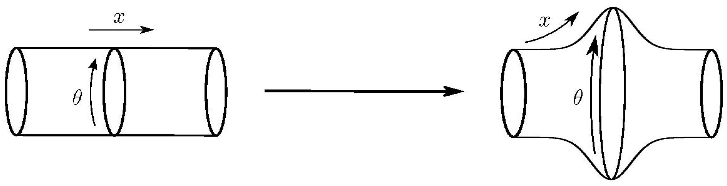
Figure 2.
The relationships between tangent space groups on product manifolds (reproduced from [6] with kind permission of World Scientific Publishing Co Pte Ltd)
Figure 2.
The relationships between tangent space groups on product manifolds (reproduced from [6] with kind permission of World Scientific Publishing Co Pte Ltd)
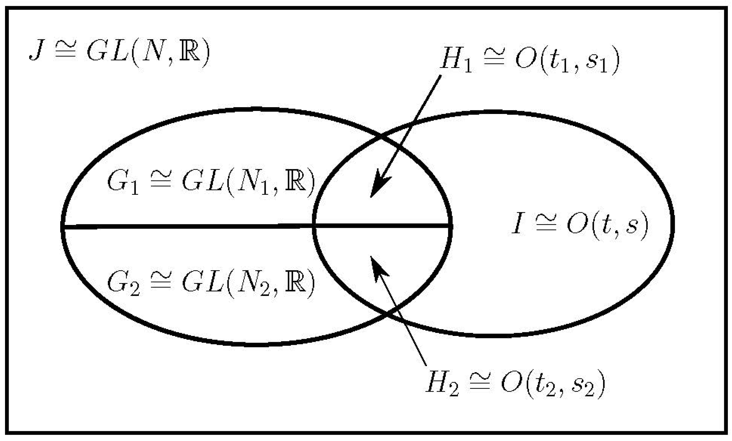

Table 1.
Comparison of the properties of the Levi-Civita and Weitzenböck connections.
| Levi-Civita | Weitzenböck |
|---|---|
| Used in GR | Used in teleparallel theories |
| Metric-compatible | Metric-compatible |
| Symmetric on lower indices: | Has torsion: |
| For given coordinate system, uniquely defined across coordinate neighbourhood, in terms of metric | For a given coordinate system, not unique – depends on choice of parallelism; defined in terms of matrices |
| Parallel transport along segments of different geodesics don’t commute – so result depends on path | Uniquely defined once coordinates and parallelism are chosen – then parallel transport is independent of path taken |
Disclaimer/Publisher’s Note: The statements, opinions and data contained in all publications are solely those of the individual author(s) and contributor(s) and not of MDPI and/or the editor(s). MDPI and/or the editor(s) disclaim responsibility for any injury to people or property resulting from any ideas, methods, instructions or products referred to in the content. |
© 2025 by the authors. Licensee MDPI, Basel, Switzerland. This article is an open access article distributed under the terms and conditions of the Creative Commons Attribution (CC BY) license (http://creativecommons.org/licenses/by/4.0/).
Copyright: This open access article is published under a Creative Commons CC BY 4.0 license, which permit the free download, distribution, and reuse, provided that the author and preprint are cited in any reuse.


