Predicting the Growth of Vibrio parahaemolyticus in Oysters Under Varying Ambient Temperature

1. Introduction

Oysters, traditionally harvested for thousands of years, are a very important part of many diets around the world [1], and increasing as aquaculture oyster demands surge [2]. Since 2009, the global production has increased from 3 million to over 5.9 million tons [3]. This is an important factor contributing to the increase in the number of cases of gastroenteritis caused by the human pathogen Vibrio parahaemolyticus (Vp) [4,5], a bacteria endemic to marine environments and present in seafood including oysters [6]. In addition to gastroenteritis, consuming oysters with high Vp concentrations can lead to primary septicemia in individuals with underlying medical conditions such as chronic diseases, liver disease, or immune disorders [7].

The first outbreak of Vp was reported in Osaka (Japan) in 1950 and since then, a continuing rise of Vp infections has been reported in several countries over the past few decades [8,9,10]. Such Vp cases increase is connected to an unknown occurrence of global Vibrio infections [11]. In 2020, around half a million Vp infection cases were estimated worldwide [10], being this pathogen the leading cause of seafood-derived illnesses worldwide [12].

It is almost impossible to obtain seafood free of these bacteria due to the ubiquitous nature of Vibrio species in marine and estuarine environments, particularly during warm, summer months [13] and the accumulation of Vibrio by oysters through filter-feeding. Seawater temperature is a major factor determining the concentration, distribution, and proliferation of Vp in the coastal environment [13,14]. Higher densities of Vp in oysters have been detected in the spring and summer, and are positively correlated with seawater temperature [13,15]. Vp is rarely detected during winter when Vibrio survives in the marine sediment until temperatures rise again to 14ºC and it is released to the seawater [2]. Oysters harvested in summer can be associated with Vp tissue concentrations approaching 1000 CFU/g, while in winter this concentration decreases to less than 10 CFU/g [13,16].

Oysters are harvested, sacked, and left at ambient air temperature on the boat deck before being dragged to shore. When the air temperature is very high in hot summer conditions, this exposure can result in an important Vp growth in oysters up to 50 × 10⁶ cells/g (7.7 $lo{g}_{10}$ CFU/g) [17]. Regarding disease risk, the probability of illness is relatively low in winter ($\le 0.00001$) for consumption of a serving of 12 oysters with 100 × 10³ Vp cells ($\sim 50$ cells/g or 1.7 $lo{g}_{10}$ CFU/g ) [18]. However, in summer this probability can increase to $\ge 0.5$ after the consumption of a serving with 100 × 10⁶ Vp cells (∼ 500 × 10³ cells/g or 5.7 $lo{g}_{10}$ CFU/g) [18]. In this context, raising temperature associated with climate change is a factor of concern, due to the expected influence of prolonged exposure to seawater temperatures supporting Vibrio proliferation and its impact on Vp distribution [10,11] and population dynamics, and eventually the impact on human disease outcomes.

To address this risk, worldwide sanitation programs for shellfish control established time-to-temperature regulations to limit the growth of Vp in post-harvest oysters [19]. An example of this thermal process consists of cooling down the shellfish harvested for raw consumption to 10ºC (50ºF) within 10, 12, or 36 hours when the average monthly air temperature is higher than 27ºC, between 19 and 27ºC or lower than 18ºC, respectively [2]. An absence of refrigeration, non-rapid refrigeration, or breaking the cold chain can lead to high temperatures during oyster warehousing leading to Vp in vivo population increase. Resubmersion can also be considered a method for vibrio control [20]

This effect of temperature on Vp has been commonly explored by experiments at different constant temperatures [17,21,22]. However, inferring outcomes from constant-temperature experiments onto realistic varying temperature regimes is complex and problematic [23]. Improving methods in this regard is essential for the understanding of this and similar temperature-dependent host-pathogen systems while supporting studies about the public health impact of pathogenic Vp associated with raw seafood consumption [17,19,24].

In this study, a continuous-time model was developed for predicting the growth of Vp in oysters under varying ambient temperatures. The model was constructed by numerically integrating an ordinary differential equation system with temperature-dependent growth parameters. First, the model was fitted, verified, and evaluated against previous experimental data of Vp concentrations in Pacific oysters (Crassostrea gigas) at constant temperatures [17]. Once the model was verified and evaluated, Vp dynamics in oysters were modeled at different post-harvest scenarios under varying environmental temperatures for winter and summer initial conditions, and with and without dockside ice and onboard ice treatments.

2. Materials and Methods

The predictive model developed in this study for exploring Vp growth in oysters under varying environmental temperatures was parameterized with and evaluated against experimental data of Vp concentrations in Pacific oysters obtained at different constant temperatures (see details in [17]). First, linear and non-parametric regression models were obtained. Second, from the maximum slopes of these models, the inactivation and growth rates were estimated. Third, using these rates, our growth model was constructed for predicting the growth of Vp in oysters under varying ambient temperatures:

2.1. OLS and LOESS Regression Models for Vp Growth and Inactivation Processes

Two models were applied to analyze the relationship of Vp concentration in oysters with time at experimental constant temperatures [17]: the classic parametric Ordinary Least Squares regression model (OLS) (Galton, 1886) and the non-parametric Locally Weighted Least Squares Regression smoothing technique (LOESS) (Cleveland et al., 1988). As a non-parametric smoothing technique, the LOESS can model the relationship between Vp and time more robustly and in a more flexible manner than parametric models such as the OLS, potentially extracting information (e.g. ecological, biological) from the data that more restrictive parametric models miss. For Vp inactivation, the goodness of fit of the OLS and LOESS regression curves were assessed and compared by analyzing the percentage error ($PE$); a lower $PE$ meaning a better prediction accuracy. The $PE$ was calculated based on the residual standard error ($RSE$) as follows:

$$\begin{array}{c}\hfill RSE=\sqrt{\frac{{\sum }_{i=1}^n(VP{C}_i-\widehat{VP{C}_i})}{n}}\end{array}$$

(1)

$$\begin{array}{c}\hfill PE(\%)=100·\frac{RSE}{\overline{VPC}}\end{array}$$

(2)

Where $VP{C}_i$ and $\widehat{VPC}$ are respectively the observed Vp and mean Vp counts in terms of colony forming units ($lo{g}_{10}$$CFU/g$) and $\widehat{VP{C}_i}$ is the predicted counts by the OLS and LOESS models.

For Vp growth, the goodness of fit of the LOESS regression curve was assessed. The obtained curves and the corresponding maximum slopes or growth rates were compared to the curves obtained by model fitting in [17]. The PE was also calculated here based on the residual standard error.

Data analysis was conducted with R statistical software (R Core Team, 2018). The “ggplot2” package was used to generate plots.

2.2. Growth and Inactivation Rates for the Model

For Vp growth, the classic square root model [25] was applied to describe the growth rate (r) as a function of temperature as follows:

$$\begin{array}{c}\hfill \sqrt{r}=a·(T-T_{min}).\end{array}$$

(3)

The model shows a linear relationship between temperature (T) and the $\sqrt{r}$, where the regression coefficient is represented by a and $T_{min}$ is a hypothetical reference or threshold temperature between growth and inactivation of Vp.

The Arrhenius equation was used for the estimation of the kinetic parameters for the effect of temperature on bacterial inactivation as follows:

$$\begin{array}{c}\hfill lnr=lnA-\frac{E_a}{R·T}\end{array}$$

(4)

where r is the reaction rate coefficient or constant, T is the absolute temperature, $E_a$ is the activation energy (i.e., the minimum amount of energy that must be provided to result in a reaction), R is the universal gas constant, and A is the collision factor.

2.3. The Model

2.3.1. Model Description, Mathematical Theory and Assumptions

The model developed here is a Vp growth model for Vp in oysters that accounts for the effect of varying temperature on bacterial growth. It is a continuous-time model, which results from an ordinary differential equation (ODE) system solved using a fourth-order Runge-Kutta method (RK4) [26]. The numerical model for this ODE system is programmed in Matlab.

The model accounts for both bacterial growth and inactivation. Regarding bacterial growth, the model is an extension of the Logistic model [27] which suggests that the rate of bacterial population increase is limited. The logistic model combines the ecological processes of growth and competition. Both processes depend on population density and their rates match the mass-action law [27]. Regarding bacterial inactivation, the model is a linear decreasing model.

2.3.2. Model Equations

Vp growth and inactivation are described by the system and conditions defined by equations (5) and (6), being $N=N_1+N_2$ the total number of Vp counts per gram. That is, for having both Vp growth and inactivation in the equation system for the variable Vp population in oysters is divided into two classes $N_1$ and $N_2$. The following equations represent the change of these two classes with time:

$$\begin{array}{c}\hfill \frac{d{N}_1}{dt}=-\gamma {\mu }_{max}{N}_1\end{array}$$

(5)

$$\begin{array}{c}\hfill \frac{d{N}_2}{dt}=\gamma {\mu }_{max}m{N}_1+{\mu }_{max}{N}_2(1-\frac{m(N_1+N_2)}{N_{max}},\end{array}$$

(6)

where ${\mu }_{max}$ is the maximum growth rate of Vp population in oysters ($cells/h$). $N_{max}$ accounts for substrate competition, that is, represents the carrying capacity or the maximum total counts, corresponding to 5.5 $lo{g}_{10}$$CFU/g$ for lower temperatures ($T<{23}^{\circ }C$), 7.5 $lo{g}_{10}$$CFU/g$ for medium-high temperatures (${23}^{\circ }C\le T<{30}^{\circ }C$) and 6.75 $lo{g}_{10}$$CFU/g$ for high temperatures ($T\ge {30}^{\circ }C$) as observed by [17]. The parameter m can be 1 or 0, depending on the temperature (see equations (7) and (8)).

From equations (3) and (4), the following growth rates (${\mu }_{max}$) were obtained:

$$\begin{array}{c}\hfill \mathrm{if}T>T_{min},{\mu }_{max}=a^2(T-T_{min})\mathrm{and}m=1\end{array}$$

(7)

$$\begin{array}{c}\hfill \mathrm{if}T\le T_{min},{\mu }_{max}=e^{lnA-\frac{E_a}{R·T}}\mathrm{and}m=0\end{array}$$

(8)

The growth rate ${\mu }_{max}$ and m depend on temperature (T) representing growth or inactivation of Vp in oysters. That is, when T is higher than $13.{37}^{\circ }C$, Vp population growth is defined by equation (7), being m=1 so that the first term in both equations (5) and (6) are annulled. In these conditions, the model studies the change in total Vp population $N=N1+N2$ or bacterial growth by the second term in equation (6), ${\mu }_{max}{N}_2(1-\frac{m(N_1+N_2)}{N_{max}})$. While if T is lower or equal to $13.{37}^{\circ }C$, the growth rate ${\mu }_{max}$ is defined by equation (8), being m=0. In this conditions, the change in total Vp population ($N=N1+N2$ or inactivation is only defined by $-\gamma {\mu }_{max}{N}_1$ in equation (5). The rest of the terms are annulled when $m=0$ and the initial number of $N_2=0$.

2.3.3. Model Verification and Evaluation

The probability of illness is relatively low ($<0.001$ percent) for consumption of 10 × 10³ cells/g Vp cells/serving [18], being a serving of 12 oysters or approximately 16 grams of meat. This is equivalent to about 50 cells/oyster meat gram; that is, 800 cells/serving. These concentrations are equivalent to winter CFU/g values [13]. However, the probability of disease increases to 50 percent for consumption of about 100 × 10⁶ Vp cells/serving. This corresponds to 8000 × 10³ cells/oyster [18], which are body burdens of the same order of magnitude as those found in oysters harvested in summer [13].

Model verification consisted of showing that the model is correct, complete, and coherent by means of (i) static tests involving a structured examination of the formulas, algorithms, and code used to implement the model, and (ii) dynamic tests, where the computer program was run under different conditions to ensure that results produced were correct, according to the conceptual model, and consistent with expectations of reviewers experts in oyster pathology, Vp and population dynamics.

The parameter values used for model verification were those obtained by fitting the model growth and inactivation rate equations (Equations 5 and 6). The model was run for a series of 100/150-hour simulations for growth scenarios and 300/500-hour simulations for inactivation scenarios. This simulation time span was chosen (i) to detect pathogen proliferation and inactivation events, and (ii) to evaluate the model against growth and inactivation experimental data along the same time span [17]. Thus, eight realistic (experimental) scenarios were simulated to verify and evaluate the performance of the model regarding the dynamics of Vp population (Table 1) [17]. Figure 3 and Figure 4 illustrate the results of these verification/evaluation cases (simulations 1-8).

2.3.4. Modelling Scenarios

Different simulations were run representing both (i) realistic environmental (air) temperatures for regions with hot summers and mild winters as in south Europe [?] and south US [?], and (ii) realistic oyster processing temperature scenarios in terms of refrigeration by ice treatment from harvesting to consumption, in both summer and winter (simulations 9-17). For each season, simulated scenarios were differentiated by the ice treatment applied to oysters: non-iced (NI), dockside ice storage (DS), on-board ice storage (OB). In the NI scenario, there is not any type of pre-consumption treatment in terms of refrigeration. In the DS scenario, ice treatment started 10 hours after harvesting. In the OB scenario, ice treatment starts onboard right after harvesting.

Table 1. Simulations for model verification and evaluation against experimental data of Vp growth at constant temperatures from laboratory tests [17].

Simulation	Scenario (Initial Conditions)	Expected Results	Figure
Simulation 1	T=18.4ºC, Vp=3.4 $lo{g}_{10}CFU/g$	Logistic (extension) 3.4 to 5.5 $lo{g}_{10}CFU/g$	3A
Simulation 2	T=20ºC, Vp=3.4 $lo{g}_{10}CFU/g$	Logistic (extension) 3.4 to 5.5 $lo{g}_{10}CFU/g$	3B
Simulation 3	T=25.7ºC, Vp=3.4 $lo{g}_{10}CFU/g$	Logistic (extension) 3.4 to 7.5 $lo{g}_{10}CFU/g$	3C
Simulation 4	T=30.4ºC,Vp=3.4 $lo{g}_{10}CFU/g$	Logistic (extension) 3.4 to 6.75 $lo{g}_{10}CFU/g$	3D
Simulation 5	T=3.6ºC, Vp=5.8 $lo{g}_{10}CFU/g$	Linear 5.8 to 3.0 $lo{g}_{10}CFU/g$	4A
Simulation 6	T=6.2ºC Vp=5.5 $lo{g}_{10}CFU/g$	Linear 5.5 to 4.0 $lo{g}_{10}CFU/g$	4B
Simulation 7	T=9.6ºCVp=5.1 $lo{g}_{10}CFU/g$	Linear 5.1 to 3.0 $lo{g}_{10}CFU/g$	4C
Simulation 8	T=12.6ºCVp=5.3 $lo{g}_{10}CFU/g$	Linear 5.3 to 4.0 $lo{g}_{10}CFU/g$	4D

Table 1. Simulations for model verification and evaluation against experimental data of Vp growth at constant temperatures from laboratory tests [17].

Simulation	Scenario (Initial Conditions)	Expected Results	Figure
Simulation 1	T=18.4ºC, Vp=3.4 $lo{g}_{10}CFU/g$	Logistic (extension) 3.4 to 5.5 $lo{g}_{10}CFU/g$	3A
Simulation 2	T=20ºC, Vp=3.4 $lo{g}_{10}CFU/g$	Logistic (extension) 3.4 to 5.5 $lo{g}_{10}CFU/g$	3B
Simulation 3	T=25.7ºC, Vp=3.4 $lo{g}_{10}CFU/g$	Logistic (extension) 3.4 to 7.5 $lo{g}_{10}CFU/g$	3C
Simulation 4	T=30.4ºC,Vp=3.4 $lo{g}_{10}CFU/g$	Logistic (extension) 3.4 to 6.75 $lo{g}_{10}CFU/g$	3D
Simulation 5	T=3.6ºC, Vp=5.8 $lo{g}_{10}CFU/g$	Linear 5.8 to 3.0 $lo{g}_{10}CFU/g$	4A
Simulation 6	T=6.2ºC Vp=5.5 $lo{g}_{10}CFU/g$	Linear 5.5 to 4.0 $lo{g}_{10}CFU/g$	4B
Simulation 7	T=9.6ºCVp=5.1 $lo{g}_{10}CFU/g$	Linear 5.1 to 3.0 $lo{g}_{10}CFU/g$	4C
Simulation 8	T=12.6ºCVp=5.3 $lo{g}_{10}CFU/g$	Linear 5.3 to 4.0 $lo{g}_{10}CFU/g$	4D

Other four realistic scenarios of interest were run in order to explore Vp how Vp growth would behave in an event of a potential break in the cold chain (simulations 18-21) referring to dockside and on-board situations in both winter and summer. Last simulation represent Vp inactivation scenario in the long term. The characteristics of this set of modeling scenarios are summarized in Table 2 and results showed in Figure 5, Figure 6, Figure 7, Figure 8, Figure 9 and Figure 10.

Table 2. Realistic scenarios for exploring Vp dynamics in oysters under varying temperature in terms of water and air temperature, ice treatment and initial Vp number per oyster gram. Ice treatments are as follows: NI (non-iced), DS (ice treatment on dockside), OB (on-board ice treatment), Breaking cold chain (BCC). Water temperature (W), Air temperature (A).

Simulation	Scenario (Initial Conditions)	Figure
Simulation 9	NI, Summer, W= ${30}^{\circ }C$, A= ${40}^{\circ }C$, Vp=3 $lo{g}_{10}CFU/g$	5A
Simulation 10	DS, Summer, W= ${30}^{\circ }C$, A= ${40}^{\circ }C$, Vp=3 $lo{g}_{10}CFU/g$	5B
Simulation 11	OB, Summer, W= ${30}^{\circ }C$, A= ${40}^{\circ }C$ , Vp=3 $lo{g}_{10}CFU/g$	5C
Simulation 12	NI, Summer, W= ${25}^{\circ }C$, A= ${30}^{\circ }C$, Vp= 3 $lo{g}_{10}CFU/g$	6A
Simulation 13	DS, Summer, W= ${25}^{\circ }C$, A= ${30}^{\circ }C$, Vp= 3 $lo{g}_{10}CFU/g$	6B
Simulation 14	OB, Summer, W= ${25}^{\circ }C$, A= ${30}^{\circ }C$ , Vp= 3 $lo{g}_{10}CFU/g$	6C
Simulation 15	NI, Winter, W= ${15}^{\circ }C$, A= ${13}^{\circ }C$, Vp= 1 $lo{g}_{10}CFU/g$,	7A
Simulation 16	DS, Winter, W= ${15}^{\circ }C$, A= ${13}^{\circ }C$, Vp= 1 $lo{g}_{10}CFU/g$,	7B
Simulation 17	OB, Winter, W= ${15}^{\circ }C$, A= ${13}^{\circ }C$, Vp= 1 $lo{g}_{10}CFU/g$,	7C
Simulation 18	DS, BCC Summer, W= ${30}^{\circ }C$, A= ${40}^{\circ }C$, Vp= 3 $lo{g}_{10}CFU/g$	8A
Simulation 19	OB, BCC, Summer, W= ${30}^{\circ }C$, A= ${40}^{\circ }C$, Vp= 3 $lo{g}_{10}CFU/g$	8B
Simulation 20	DS, BCC, Winter, W= ${15}^{\circ }C$, A= ${13}^{\circ }C$, Vp= 1 $lo{g}_{10}CFU/g$	9A
Simulation 21	OB, BCC, Winter, W= ${15}^{\circ }C$, A= ${13}^{\circ }C$, Vp= 1 $lo{g}_{10}CFU/g$	9B
Simulation 22	DS, Summer, W= ${25}^{\circ }C$, A= ${30}^{\circ }C$, Vp= 3 $lo{g}_{10}CFU/g$	10A

Table 2. Realistic scenarios for exploring Vp dynamics in oysters under varying temperature in terms of water and air temperature, ice treatment and initial Vp number per oyster gram. Ice treatments are as follows: NI (non-iced), DS (ice treatment on dockside), OB (on-board ice treatment), Breaking cold chain (BCC). Water temperature (W), Air temperature (A).

Simulation	Scenario (Initial Conditions)	Figure
Simulation 9	NI, Summer, W= ${30}^{\circ }C$, A= ${40}^{\circ }C$, Vp=3 $lo{g}_{10}CFU/g$	5A
Simulation 10	DS, Summer, W= ${30}^{\circ }C$, A= ${40}^{\circ }C$, Vp=3 $lo{g}_{10}CFU/g$	5B
Simulation 11	OB, Summer, W= ${30}^{\circ }C$, A= ${40}^{\circ }C$ , Vp=3 $lo{g}_{10}CFU/g$	5C
Simulation 12	NI, Summer, W= ${25}^{\circ }C$, A= ${30}^{\circ }C$, Vp= 3 $lo{g}_{10}CFU/g$	6A
Simulation 13	DS, Summer, W= ${25}^{\circ }C$, A= ${30}^{\circ }C$, Vp= 3 $lo{g}_{10}CFU/g$	6B
Simulation 14	OB, Summer, W= ${25}^{\circ }C$, A= ${30}^{\circ }C$ , Vp= 3 $lo{g}_{10}CFU/g$	6C
Simulation 15	NI, Winter, W= ${15}^{\circ }C$, A= ${13}^{\circ }C$, Vp= 1 $lo{g}_{10}CFU/g$,	7A
Simulation 16	DS, Winter, W= ${15}^{\circ }C$, A= ${13}^{\circ }C$, Vp= 1 $lo{g}_{10}CFU/g$,	7B
Simulation 17	OB, Winter, W= ${15}^{\circ }C$, A= ${13}^{\circ }C$, Vp= 1 $lo{g}_{10}CFU/g$,	7C
Simulation 18	DS, BCC Summer, W= ${30}^{\circ }C$, A= ${40}^{\circ }C$, Vp= 3 $lo{g}_{10}CFU/g$	8A
Simulation 19	OB, BCC, Summer, W= ${30}^{\circ }C$, A= ${40}^{\circ }C$, Vp= 3 $lo{g}_{10}CFU/g$	8B
Simulation 20	DS, BCC, Winter, W= ${15}^{\circ }C$, A= ${13}^{\circ }C$, Vp= 1 $lo{g}_{10}CFU/g$	9A
Simulation 21	OB, BCC, Winter, W= ${15}^{\circ }C$, A= ${13}^{\circ }C$, Vp= 1 $lo{g}_{10}CFU/g$	9B
Simulation 22	DS, Summer, W= ${25}^{\circ }C$, A= ${30}^{\circ }C$, Vp= 3 $lo{g}_{10}CFU/g$	10A

2.4. Risk of Illness

The model results are discussed in terms of the probability of illness. For this, risk of illness was estimated in Table 3 by adapting previous dose-response model results [18].

Table 3. Probability and risk of gastroenteritis ((P(G) and R(G), respectively) and septicemia (P(S) and R(S), respectively) as a function of Vp dose per oyster serving (12 oysters) and per oyster gram in a serving. Adapted and estimated from results of the Beta-Poisson Dose-Response model by [18].

CFU Per Serving	Log CFU/g	P (G)	Risk (G)	P (S)	Risk (S)
${10}^4$	1.72	$1.0·{10}^{-4}$	Extremely low	$2.5·{10}^{-7}$	Extremely low
${10}^5$	2.72	$1.0·{10}^{-3}$	Very low	$2.5·{10}^{-6}$	Extremely low
${10}^6$	3.72	$1.0·{10}^{-2}$	Low	$2.5·{10}^{-5}$	Extremely low
${10}^7$	4.72	$1.0·{10}^{-1}$	Moderate	$2.5·{10}^{-4}$	Extremelylow
${10}^8$	5.72	$5.0·{10}^{-1}$	High	$1.3·{10}^{-3}$	Verylow
${10}^9$	6.72	$9.0·{10}^{-1}$	Very high	$2.3·{10}^{-3}$	Verylow
${10}^{10}$	7.72	$9.6·{10}^{-1}$	Extremely high	$2.4·{10}^{-3}$	Verylow
${10}^{11}$	8.72	$9.9·{10}^{-1}$	Extremely high	$2.5·{10}^{-3}$	Very low

Table 3. Probability and risk of gastroenteritis ((P(G) and R(G), respectively) and septicemia (P(S) and R(S), respectively) as a function of Vp dose per oyster serving (12 oysters) and per oyster gram in a serving. Adapted and estimated from results of the Beta-Poisson Dose-Response model by [18].

CFU Per Serving	Log CFU/g	P (G)	Risk (G)	P (S)	Risk (S)
${10}^4$	1.72	$1.0·{10}^{-4}$	Extremely low	$2.5·{10}^{-7}$	Extremely low
${10}^5$	2.72	$1.0·{10}^{-3}$	Very low	$2.5·{10}^{-6}$	Extremely low
${10}^6$	3.72	$1.0·{10}^{-2}$	Low	$2.5·{10}^{-5}$	Extremely low
${10}^7$	4.72	$1.0·{10}^{-1}$	Moderate	$2.5·{10}^{-4}$	Extremelylow
${10}^8$	5.72	$5.0·{10}^{-1}$	High	$1.3·{10}^{-3}$	Verylow
${10}^9$	6.72	$9.0·{10}^{-1}$	Very high	$2.3·{10}^{-3}$	Verylow
${10}^{10}$	7.72	$9.6·{10}^{-1}$	Extremely high	$2.4·{10}^{-3}$	Verylow
${10}^{11}$	8.72	$9.9·{10}^{-1}$	Extremely high	$2.5·{10}^{-3}$	Very low

Note that U.S. Food and Drug Administration [18], for example, predicts about 2800 Vp illnesses from oyster consumption each year. Of infected individuals, approximately 7 cases of gastroenteritis will progress to septicemia each year for the total population, of which 2 individuals would be from the healthy sub-population and 5 would be from the immunocompromised sub-population [18].

2.5. Model Limitations

The ODE system here was solved using the RK4 method. RK4 methods are easy to implement, very stable, and self-starting; that is, unlike multi-step methods, there is no need to treat the first few steps taken by a single-step integration method as special cases. However, the primary disadvantages of RK4 methods are (i) the requirement of significantly more computation time than multi-step methods of comparable accuracy, and (ii) the fact that they do not easily yield good global estimates of the truncation error. However, for straightforward dynamical systems such as the one investigated by this model, the advantage of the relative simplicity and ease of use of RK4 methods far outweighs the disadvantage of their relatively high computational cost.

The growth and inactivation rate for the model was obtained by integrating the information obtained by regression models exploring the change in Vp concentrations with time at only eight constant temperatures. This is a simplification of reality and may result in a relative underestimation of Vp growth and consequently is an underestimation of the risk of getting gastroenteritis and septicemia.

Finally, when modeling realistic scenarios caution is required to interpret the results in quantitative terms; since the model is dealing with multiple dimensions, latent covariates, and data coming from laboratory experiments could result in some situations that are not entirely realistic.

3. Results

3.1. $OLS$ and $LOESS$ Regression Models for Vp Growth and Inactivation

For Vp growth, at higher temperatures (18.4${ }^{\circ }$C, 20.0${ }^{\circ }$C, 25.7${ }^{\circ }$C and 30.4${ }^{\circ }$C), the LOESS model expresses the Vp growth in a more flexible manner than that obtained by the Baranyi model [17]. The maximum Vp count level beyond which the Vp counts remain constant in the Baranyi model [17] is not that clear and constant for the LOESS model here, showing some increasing patterns beyond that level (Figure 1, A-D). Nevertheless, comparing maximum growth rates (initial slopes) in terms of $lo{g}_{10}CFU/h$ there are no differences.

For Vp inactivation, OLS regression models from experiments [17] showed significant (p<0.05) negative linear relationships of Vp counts ($CFU/g$) with time for different constant temperatures between 3.6${ }^{\circ }$C and 12.6${ }^{\circ }$C (Figure 2 A-D, left). The Pearson correlation coefficient squared was high in all cases ($R^2$ between 0.769 and 0.913). The LOESS regression curves showed that the response variable Vp counts exhibited a progressive inactivation (decrease) with time (Figure 2 A-D, right). Particularly, for 6.2${ }^{\circ }$C and 12.6${ }^{\circ }$C, this inactivation showed two phases: the inactivation in the first phase was faster than that in the second phase. These LOESS curves adapted in a more flexible manner to data, however, the differences in PE were not significant and inactivation rates in terms of $lo{g}_{10}CFU/h$ can be considered similar. The OLS and LOESS showed similar $PE$, 3.36-8.6% and 3.24-8.89%, respectively. Regarding the goodness of fit, all studied models were well-fitting regression models ($PE$<10%).

Figure 1. $LOESS$ regression model for 18.4, 20.0, 25.7, and 30.4ºC. Regression curves are represented by solid lines with smoothing based on 95% confidence intervals (shaded areas).

Figure 1. $LOESS$ regression model for 18.4, 20.0, 25.7, and 30.4ºC. Regression curves are represented by solid lines with smoothing based on 95% confidence intervals (shaded areas).

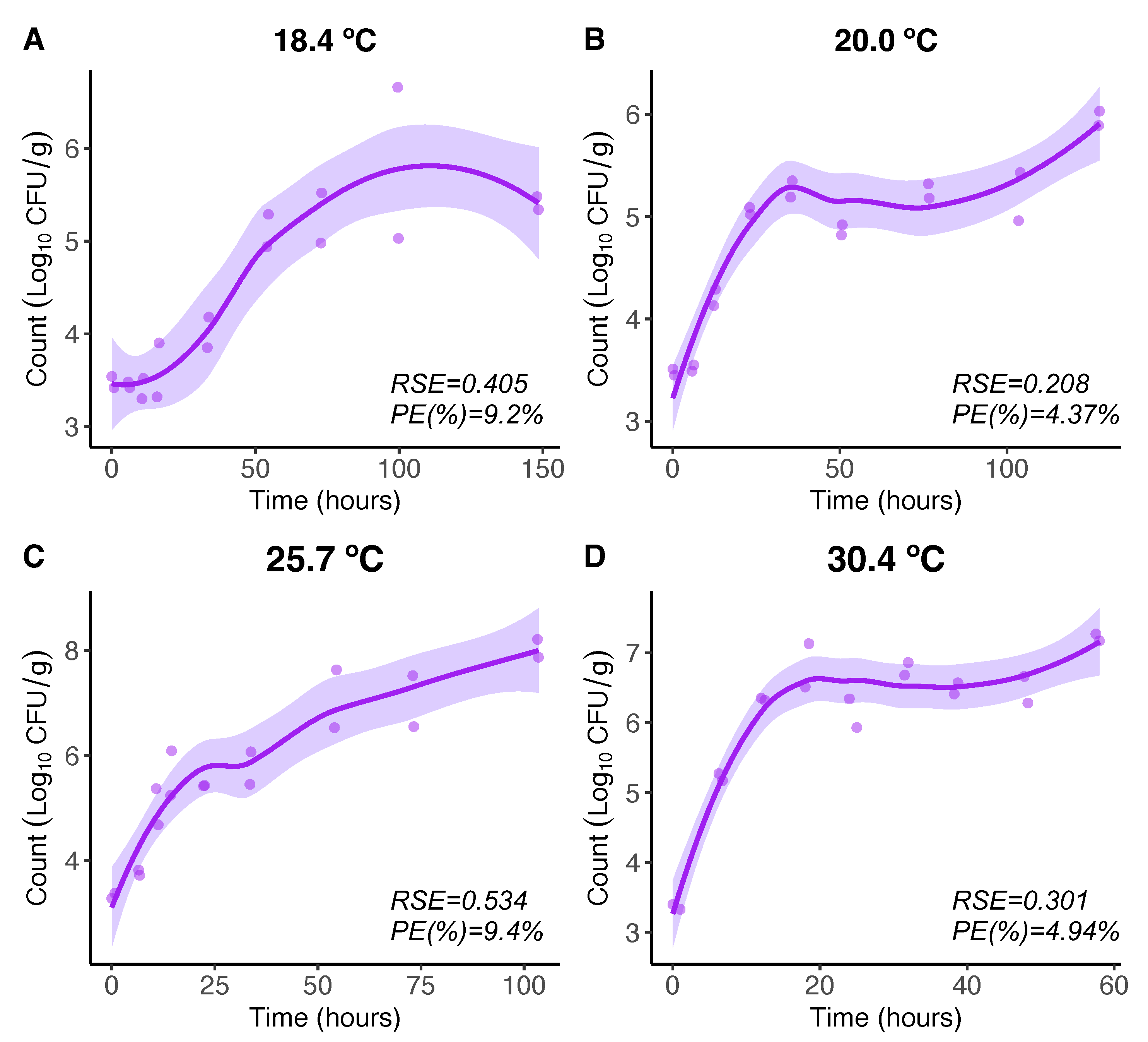
Figure 2. $OLS$ and $LOESS$ regression models for 3.6, 6.2, 9.6, and 12.6ºC. Regression curves are represented by solid lines with smoothing based on 95% confidence intervals (shaded areas).

Figure 2. $OLS$ and $LOESS$ regression models for 3.6, 6.2, 9.6, and 12.6ºC. Regression curves are represented by solid lines with smoothing based on 95% confidence intervals (shaded areas).

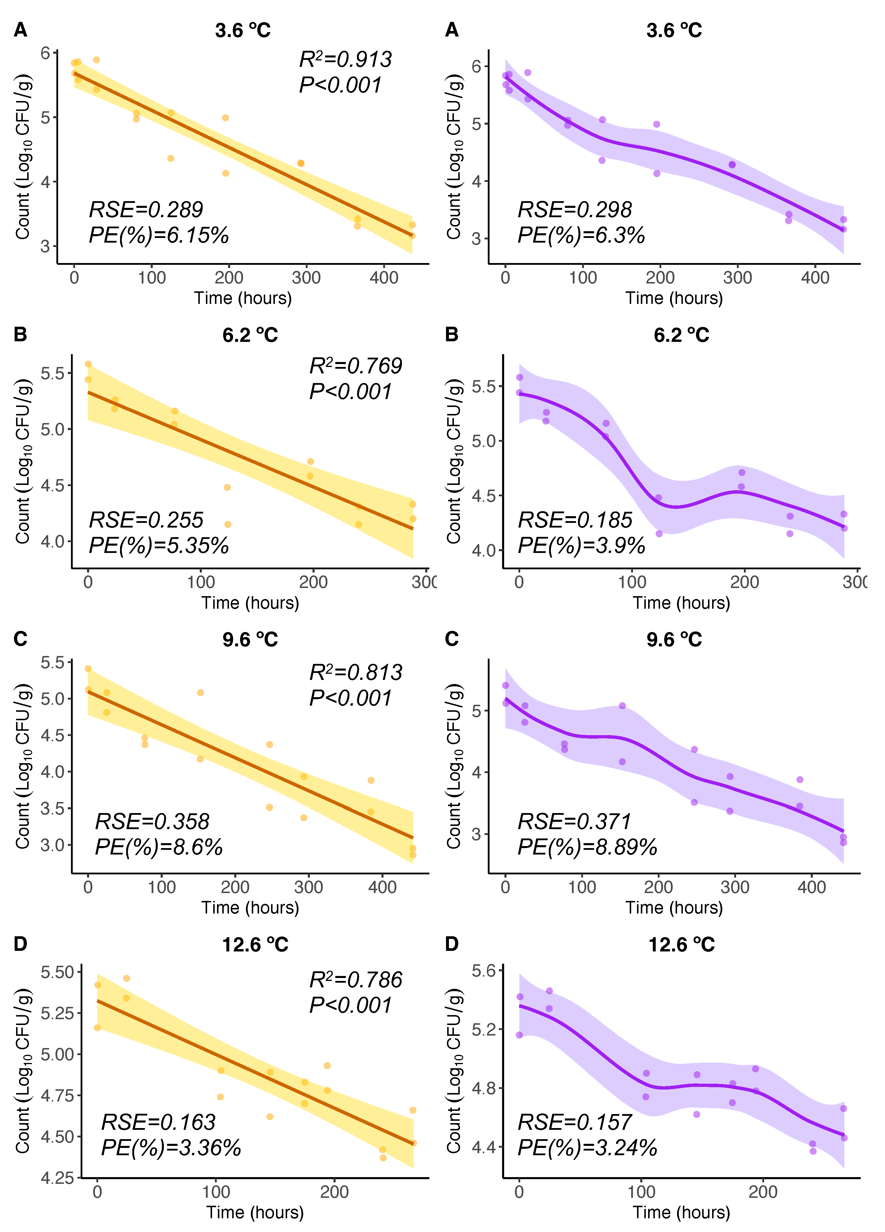
The results of this comparative analysis between both the OLS and Baranyi models applied in [17] and the LOESS models here, suggest to use similar maximum growth rate values (slopes) for each temperature as in [17] in order to formulate the equations (models) for growth and inactivation rates needed for the Vp growth model in oysters developed here.

3.2. Growth and Inactivation Rates for the Model

From OLS and LOESS regression models (slopes) maximum growth and inactivation rates for Vp were obtained as in [17]. These rates were -0.006, -0.004, -0.005, -0.003, 0.030, 0.075, 0.095, and 0.282 $lo{g}_{10}CFU/h$ at 3.6, 6.2, 9.6, 12.6, 18.4, 20.0, 25.7, and 30.4ºC, respectively. Fitting these rates vs different temperatures, the following parameter values for equations 1 and 2 were obtained: $T_{min}$=13.37ºC, as an intrinsic property of the Pacific oyster, and $a=0.04$, $A=4.81·{10}^{-9}$, $E_a=4131.2$, $R=T+273.5$. Thus, the growth and inactivation rate models as a function of temperature were formulated as follows:

For Vp growth, the classic square root model [25] applied to describe the growth rate is formulated as:

$$\begin{array}{c}\hfill \sqrt{r}=0.04·(T-13.37).\end{array}$$

(9)

The model for growth shows a linear relationship between temperature (T) and the $\sqrt{r}$, where the regression coefficient is represented by a, and $T_{min}$ is a hypothetical reference or threshold temperature between growth and inactivation of Vp. As an intrinsic property of the Pacific oyster, this temperature is $T_{min}=13.{37}^{\circ }C$ [17].

The Arrhenius equation was used for the estimation of the kinetic parameters for the effect of temperature on bacterial inactivation. The equation used was as follows:

$$\begin{array}{c}\hfill lnr=Ln(4.81·{10}^{-9}+4131.2·\left(\frac{1}{T+273.5}\right),\end{array}$$

(10)

where r is the rate constant, T is the absolute temperature, $E_a$ is the activation energy, R is the universal gas constant, and A is the collision factor.

3.3. Model Verification and Evaluation

Simulations at constant temperatures for model verification and evaluation (Figure 3 and Figure 4) were run with initial conditions described in Table 1 and model parameter values defined in Section 2.3.3 and Section 3.2

For growth scenarios (Simulations 1-4) results conform to expectations (Table 2.1) and thus, are consistent with real experimental data from [17] using identical initial conditions and temperatures. Increasing temperature from Figure 3A–C leads to more rapid initial growth and eventually in a higher maximum growth rate conforming to expectations (Table 1). Overall, Regarding model evaluation, the model has a very good fit to the experimental data both for the maximum growth and the Vp values at the maximum of the curve (Table 1 and [17]).

Figure 3. Simulations 1-4 from Table 2.1 (A-D) for model verification and evaluation using constant temperatures as in [17].

Figure 3. Simulations 1-4 from Table 2.1 (A-D) for model verification and evaluation using constant temperatures as in [17].

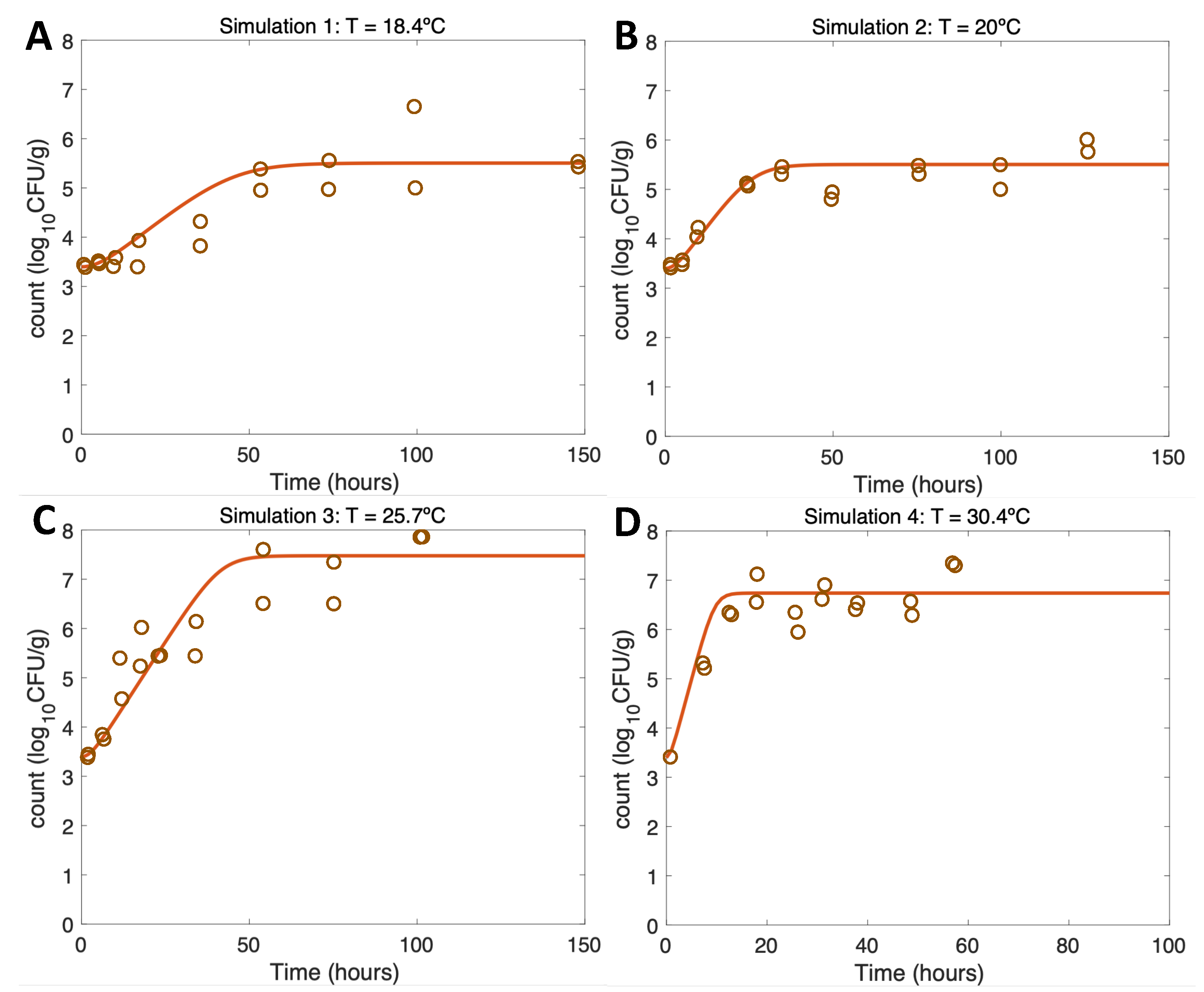
Figure 4. Simulations 5-8 from Table 2.1 (A-D) for model verification and evaluation using constant temperatures as in inactivation experiments conducted by [17].

Figure 4. Simulations 5-8 from Table 2.1 (A-D) for model verification and evaluation using constant temperatures as in inactivation experiments conducted by [17].

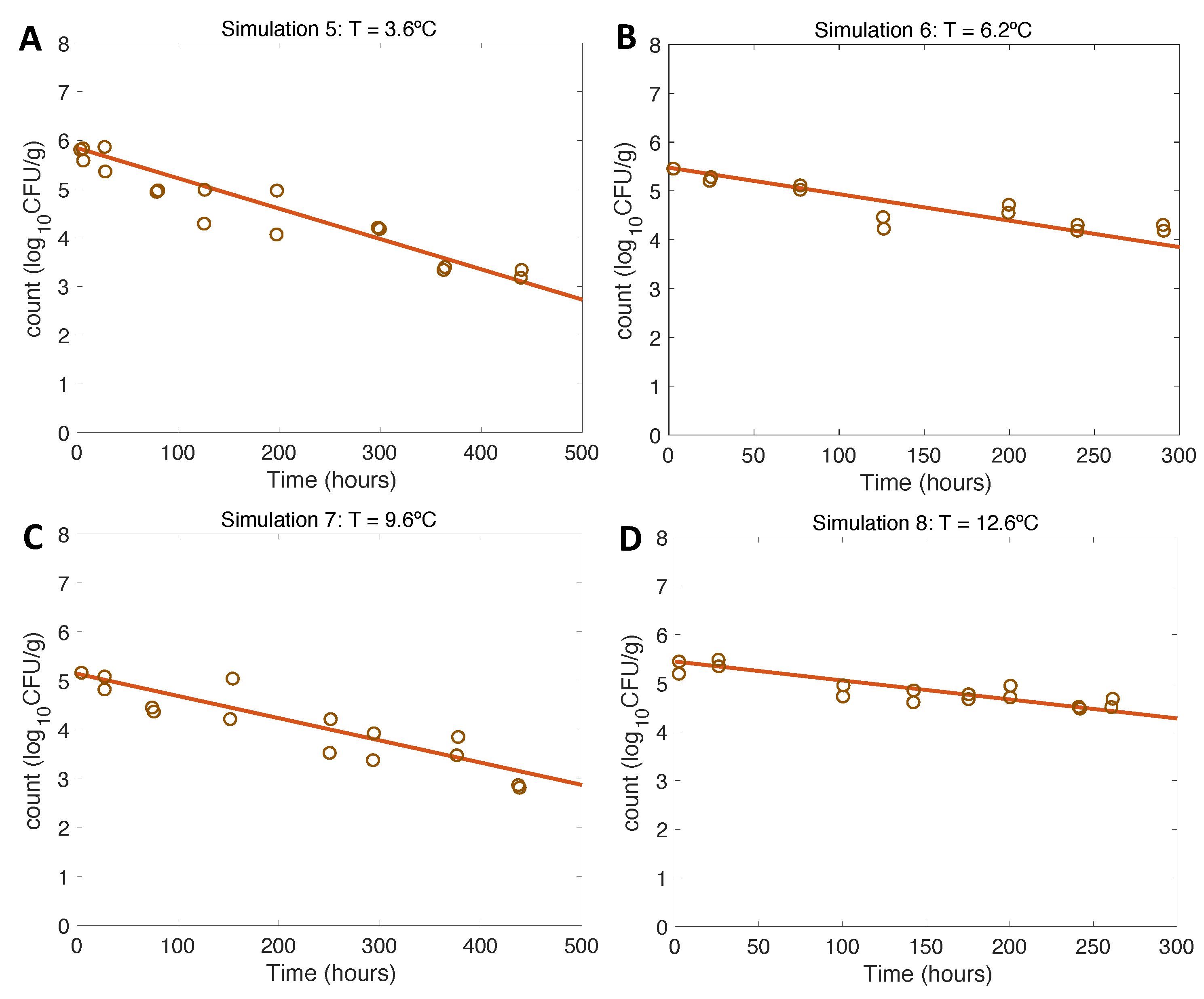
Results of model verification for inactivation scenarios conform to expectations, being also consistent experimental data from [17]. In this case, the opposite trend to growth is observed: the lower the temperature, the faster the inactivation of the pathogen conforms to the expected final values. Regarding model evaluation, the model has a very good fit to the experimental data for the entire inactivation pattern (Table 1 and [17]).

3.4. Modelling Scenarios under Varying Temperature

Once the model was verified and evaluated against real data [17], a series of theoretical scenarios were simulated, trying to mirror realistic scenarios. The results obtained for each scenario tested are described and shown in Table 2 and Figure 5, Figure 6, Figure 7, Figure 8, Figure 9 and Figure 10.

3.4.1. Simulations 9–11. Summer. Water 30${ }^{\circ }$C, Air 40${ }^{\circ }$C

In the NI scenario (Simulation 9, Figure 5A, left) the initial Vp concentration is 1000 $CFU/g$ (3 $lo{g}_{10}CFU/g$) as found by [13] in summer. The post-harvest air temperature oscillates between 18 and 40${ }^{\circ }$C mirroring day/night temperature fluctuations. Given these varying temperature conditions, a gradual increase in Vp counts is observed with a maximum of 7.5 $lo{g}_{10}CFU/g$ (Simulation 9, Figure 5A, right). Relatively low temperatures in this simulation lead to a slower growth rate. The risk of illness is high beyond hour 20 and very high beyond hour 23.

In the DS scenario (Simulation 10, Figure 5B, left), under the same initial conditions, the temperature represents an ice treatment in the dockside some hours after the harvest of oysters on board and transport to the dockside. Here, the ice treatment leads to a drastic decrease in temperature; 4 hours are necessary for the oysters at high temperature to reach a low temperature (7.2${ }^{\circ }$C) [13]. Given these temperature conditions, a gradual Vp increase is observed at the beginning of the curve, but temperatures during cold storage resulted in a slow inactivation process, reaching a maximum of 6.25 $lo{g}_{10}CFU/g$ Vp counts (Simulation 10, Figure 5 B, right). The risk of illness is high beyond hour 10 but thanks to the DS ice treatment this risk does not continue increasing and slowly decreases to hour 50.

Figure 5. Simulations 9 - 11. Summer Non-Ice (NI), Dockside (DS) and On Board (OB) post-harvest ice treatment scenarios. Water temperature of 30${ }^{\circ }$ and Air temperature of 40${ }^{\circ }$C, and initial Vp concentration of 1000 CFU/g.

Figure 5. Simulations 9 - 11. Summer Non-Ice (NI), Dockside (DS) and On Board (OB) post-harvest ice treatment scenarios. Water temperature of 30${ }^{\circ }$ and Air temperature of 40${ }^{\circ }$C, and initial Vp concentration of 1000 CFU/g.

Finally, in the OB scenario (Simulation 11, Figure 5C, left), repeating the aforementioned initial conditions, oysters are stored on ice within two hours after harvesting. Therefore, considering that oysters stored on ice reach 7.2${ }^{\circ }$C in 4 hours, beyond hour 6 of this simulation the temperature is constant. Under these temperature conditions, a slight increase in Vp counts is observed up to hour 4, after which counts start gradually to decrease, with a final total count of 3.5 $lo{g}_{10}CFU/g$ (Simulation 11, Figure 5C, right). The risk of illness in this scenario was low after the drastic inactivation caused by OB ice treatment.

3.4.2. Simulations 12–14. Summer. Water 25${ }^{\circ }$C, Air 30${ }^{\circ }$C

In the non-ice scenario (Simulation 12, Figure 6A, left) the initial Vp concentration is 1000 $CFU/g$ (3 $lo{g}_{10}CFU/g$) as found by [13] in summer. The post-harvest air temperature oscillates between 13 and 32${ }^{\circ }$C mirroring day/night temperature fluctuations. Given these varying temperature conditions, a gradual increase in Vp counts is observed with a maximum of around 6.8 $lo{g}_{10}CFU/g$ (Simulation 12, Figure 6A, right). Minimum temperatures result in slower inactivation. The risk of illness is moderate approximately beyond hour 25, high beyond hour 42, reaching the very high-risk of illness at hour 49.

Figure 6. Simulations 12 - 14. Summer Non-Ice (NI), Dockside (DS) and On Board (OB) post-harvest ice treatment scenarios. Water temeprature of 25${ }^{\circ }$ and Air temperature of 30${ }^{\circ }$C, and initial Vp concentration of 1000 CFU/g.

Figure 6. Simulations 12 - 14. Summer Non-Ice (NI), Dockside (DS) and On Board (OB) post-harvest ice treatment scenarios. Water temeprature of 25${ }^{\circ }$ and Air temperature of 30${ }^{\circ }$C, and initial Vp concentration of 1000 CFU/g.

The DS scenario (Simulation 13, Figure 6B, left) was performed under the same initial conditions aforesaid. In this scenario, oysters are initially exposed to temperatures oscillating between 25 and 32${ }^{\circ }$C. Then the temperature changes drastically by storing oysters on ice on DS for 10 hours after harvesting. 4 hours are necessary for the oysters on ice to reach a temperature of 7.2${ }^{\circ }$C, which was maintained to the end of the simulation. Temperatures during ice storage resulted in a halt in the growth, showing a final value of 4.1 $lo{g}_{10}CFU/g$ (Simulation 13, Figure 6B, right). The risk of illness increases to low risk by hour 5 and stays, with a descending pattern, in that risk zone until the end of the simulation.

Referring to the OB scenario (Simulation 14, Figure 6C, left), under identical initial conditions, after harvesting, it took 2 hours for the oysters to be stored on ice. Therefore, after cooling them down, a constant temperature was maintained from hour 6 to the end of the simulation (hour 50). A small increase of the Vp counts is observed up to hour 4, after which Vp counts start gradually to decrease, with a final total count of 3.1 $lo{g}_{10}CFU/g$ (Simulation 14, Figure 6C, right). The risk of illness in this simulation was never higher than low.

3.4.3. Simulations 15–17. Winter. Water 15${ }^{\circ }$C

First, alluding to the NI scenario (Simulation 15, Figure 7A, left) the initial Vp concentration value is 10 $CFU/g$ (3 $lo{g}_{10}CFU/g$) as found by [13] in winter. The post-harvest air temperature oscillates between 4 and 17${ }^{\circ }$C. Given these varying temperature conditions, a gradual decrease in Vp concentration is observed with 0.85 $lo{g}_{10}CFU/g$ at the end of the simulation (Simulation 15, Figure 7A, right). As temperature do not exceed 17${ }^{\circ }$C, there is no Vp growth in this scenario, so the risk of illness is very low throughout the simulation.

Continuing with the DS scenario (Simulation 16, Figure 7B, left), a similar trend is observed despite the storage on ice being 10 hours after harvesting. A slightly higher Vp inactivation than that observed in NI scenario can be noticed here, with a final Vp concentration of 0.8 $lo{g}_{10}CFU/g$ (Simulation 16, Figure 7B, right). The risk of disease also remained very low throughout the scenario. Finally, with regard to the use of ice OB, the decreasing pattern is also similar to the previous two scenarios; the use of ice after harvesting causes a decrease in the Vp counts, reaching 0.76 $lo{g}_{10}CFU/g$ (Simulation 17, Figure 7C, right). The risk of illness also remains at a very low level during the simulation time.

Figure 7. Simulations 15 - 17. Winter Non-Ice (NI), Dockside (DS) and On Board (OB) post-harvest ice treatment scenarios. Water temperature of 15${ }^{\circ }$C, and initial Vp concentration of 10 $CFU/g$.

Figure 7. Simulations 15 - 17. Winter Non-Ice (NI), Dockside (DS) and On Board (OB) post-harvest ice treatment scenarios. Water temperature of 15${ }^{\circ }$C, and initial Vp concentration of 10 $CFU/g$.

3.4.4. Other Simulations of inter-est. Simulations 18–22

In Figure 8, two previously simulated summer scenarios (DS & OB, Water 25${ }^{\circ }$C, Air 30${ }^{\circ }$C) are simulated but in this case, occurring a hypothetical break in the cold chain. Simulations 18 and 19 (Figure 8A,B, left) reproduce two cold chain break events: the first event describes oysters moved from a market to consumer (hour 24, 32${ }^{\circ }$C), and the second event, at the end of the simulation, refers to the movement of oysters from a market to a consumption site (hour 50, 29${ }^{\circ }$C). The model shows an increase in the final concentration of Vp counts, resulting in Vp concentrations of 4.7 $lo{g}_{10}CFU/g$ for the DS scenario (Figure 8A, right) and 3.7 $lo{g}_{10}CFU/g$ for the OB scenario (Figure 8B, right). The risk of illness is moderate for the DS scenario and remained low throughout the OB scenario.

Figure 8. Simulations 18 - 19. Summer Dockside (DS) and On Board (OB) post-harvest ice treatment scenarios, breaking cold chain. Water temperature of 25${ }^{\circ }$C and Air temperature od 30${ }^{\circ }$C and initial Vp concentration of 1000 $CFU/g$.

Figure 8. Simulations 18 - 19. Summer Dockside (DS) and On Board (OB) post-harvest ice treatment scenarios, breaking cold chain. Water temperature of 25${ }^{\circ }$C and Air temperature od 30${ }^{\circ }$C and initial Vp concentration of 1000 $CFU/g$.

Such breaks in cold storage were also tested in winter scenarios (Simulation 20 (DS) & Simulation 21 (OB), Water 10${ }^{\circ }$C, Air 15${ }^{\circ }$C). Although a slight rise in temperature in hours 24 and 50 was simulated due to those breaks in the cold chain (Figure 9A,B, left), here, the sudden increase in temperature led to a slight increase in Vp not compromising consumer´s health, as the risk of disease remained below the low-risk zone to the end of the simulation. (Figure 9A,B, right)

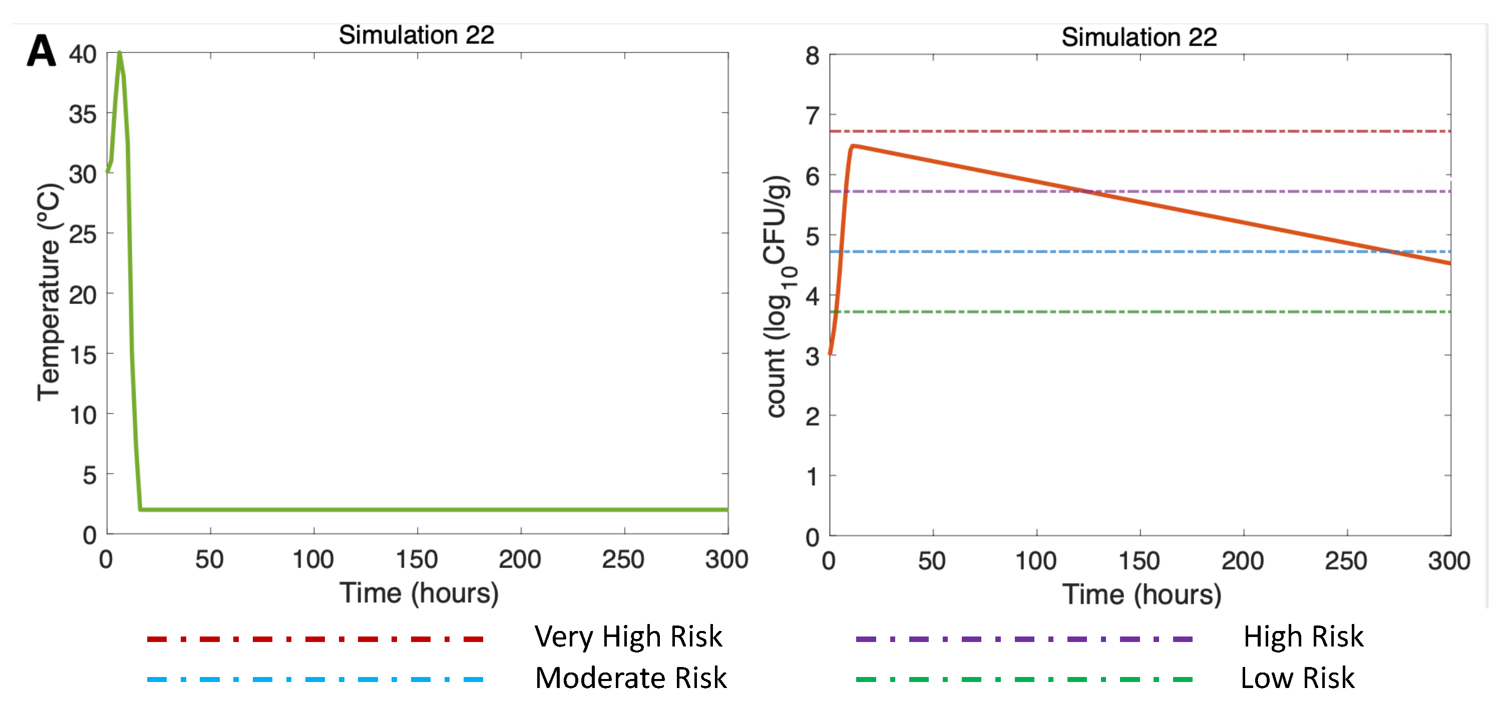
Finally, Figure 10 (DS in summer, Air 40${ }^{\circ }$C) shows how long the use of ice was necessary to reduce the risk of illness to the low-risk zone for gastroenteritis and extremely low for septicemia (Table 3). This simulation is the same as Simulation 10, (Figure 5A, right) but here applying a more prolonged ice treatment. In this simulation 22 (Figure 10A, left), oysters were subjected to cooling at 2${ }^{\circ }$C after the first 10 hours of harvesting on DS. Referring to [13], and remembering the above mentioned, the temperature scenario is constructed as follows: oysters in ice can take an average of 4 hours in summer to descend to temperatures equal to 7.2${ }^{\circ }$C, which is why a temperature equal to 2${ }^{\circ }$C is reached in hour 18. This temperature is maintained until the end of the simulation (hour 300). A gradual inactivation is observed in this simulation, ending with a Vp concentration of 4.5$lo{g}_{10}CFU/g$, implying a decrease from a high-risk zone to a low-risk zone.

Figure 9. Simulations 20 - 21. Winter Dockside (DS) and On Board (OB) post-harvest ice treatment scenarios, breaking cold chain. Water temperature of 15${ }^{\circ }$C and initial Vp concentration of 10 $CFU/g$.

Figure 9. Simulations 20 - 21. Winter Dockside (DS) and On Board (OB) post-harvest ice treatment scenarios, breaking cold chain. Water temperature of 15${ }^{\circ }$C and initial Vp concentration of 10 $CFU/g$.

Figure 10. Summer Dockside (DS) post-harvest ice treatment scenario, 300-hour duration. Water temperature of 30${ }^{\circ }$ and Air temperature of 40${ }^{\circ }$C, and initial Vp concentration of 1000 CFU/g.

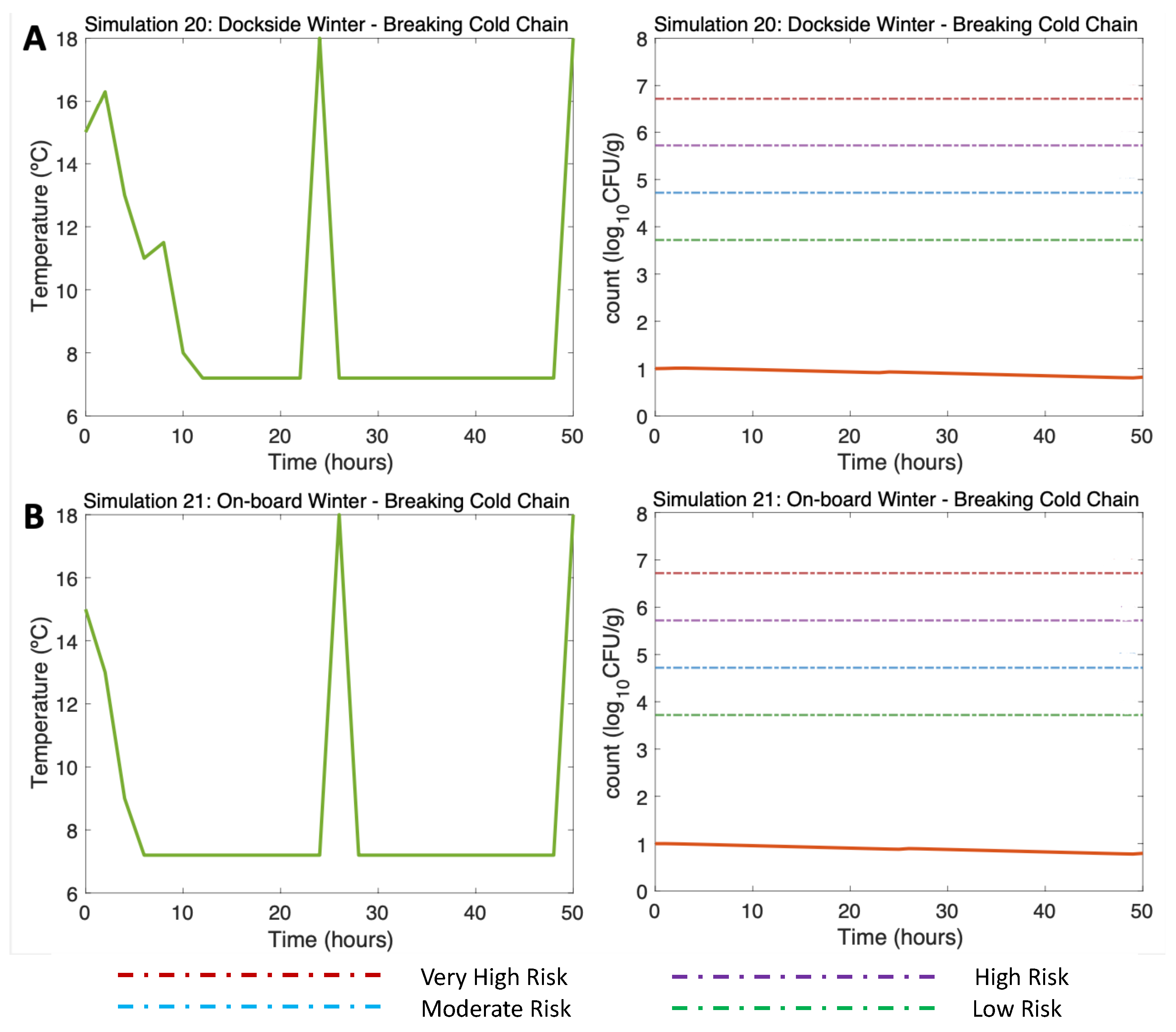
Figure 10. Summer Dockside (DS) post-harvest ice treatment scenario, 300-hour duration. Water temperature of 30${ }^{\circ }$ and Air temperature of 40${ }^{\circ }$C, and initial Vp concentration of 1000 CFU/g.

4. Discussion

Varying temperatures critically shape Vp proliferation dynamics of oysters [18,28]. However, empirically testing all possible varying temperature scenarios for a comprehensive study of their effects on Vp proliferation is unachievable. Modeling Vp growth under varying temperature mirroring ambient temperatures and the effect of ice treatments is crucial to both predict the magnitude of human illnesses and identify the temperature-related dynamics that are most important, particularly in the face of environmental change [10,29].

Our model generalizing from constant to time-varying temperatures was fed by growth and inactivation rate equations, both being temperature-dependent functions. These equations were obtained by means of analyzing the slope of regression models of the relationship between Vp counts and time under different constant temperatures obtained in previous experiments [17]. The slope for inactivation was identical to that obtained by [17] as the same linear model was applied. The slope for the growth rate (maximum slope) obtained by the nonparametric LOESS regression model was very similar to that obtained by Baranyi models in [17]. However, the LOESS curve adapted in a more flexible manner to the data and has the potential to extract more information from it than the Baranyi model. That is, the main advantage of using these types of models is the flexibility and the ease of interpretation of the smoothing function [30]. Although further biological/ecological analysis of these non-parametric curves is required, non-parametric curves seem to provide valuable information to study the dynamics of bacterial growth in oysters in detail.

The model verification results conform to expectations of mathematical theory, behavior, and population dynamics. Moreover, the model evaluation against real experimental data shows a favorable match with particularly well-documented growth and inactivation dynamics from constant-temperature experiments [17]. Once the model was verified and successfully evaluated, it can be considered for simulating different scenarios with the objective of improving the understanding of the Vp-oyster system to support studies about the public health impact of pathogenic Vp associated with raw oyster consumption. More broadly, this predictive initiative has the purpose to support identifying options for managing diseases caused by the consumption of any type of seafood. In addition, the model has also space to be adapted to and provide insights into other pathogen systems responding to varying temperatures e.g., [31].

The model here is able to incorporate varying temperature conditions and day/night temperature oscillations to reproduce their effect on the temporal dynamics of Vp. In this study, model initial conditions mirror realistic summer/winter Vp concentrations in oysters [13], with summer Vp counts well above those in winter as high-temperatures favor Vp proliferation, causing a higher number of bacteria at the time of collection. Model results are discussed here in terms of realistic air temperatures for zones with hot summers and mild winters as in south Europe [[?] and south US [?]. Increasing ambient temperature in summer favor Vp growth in oysters from 3 $lo{g}_{10}CFU/g$ up to 7.5 $lo{g}_{10}CFU/g$, resulting in a very high risk of gastroenteritis after consumption of a serving (12 oysters), particularly in hot summers reaching 40${ }^{\circ }$C (Simulation 9). The model also reflects pathogen inactivation due to day/night oscillations, particularly, due to ice treatments. Ice treatment is much more effective in limiting the risk of illness when this is applied on board compared to dockside. On board, the gastroenteritis risk decreases to the low-risk zone (Simulation 11) corresponding to an extremely low risk for sepsis (Table 3). Whilst, for dockside ice treatment, the risk of illness after a raw oyster serving consumption remains high for gastroenteritis and extremely high for septicemia. These results can be extrapolated to milder summers (30${ }^{\circ }$C) in terms of dynamic patterns (Simulations 12-14) showing a rapid increase of Vp followed by a maximum plateau. However, in this case, both on-board and dockside ice treatments limit the disease risk to the low-risk zone.

The model results are realistic; consuming raw oysters during hot summer months is inherently risky and requires onboard icing, while in mild summers dockside ice can be an acceptable control measure. The benefit of ice in hot summer scenarios is clear in our model results, but it should be emphasized that late cooling of oysters can be fatal and may not sufficiently inactivate the Vp generated in the first few hours for guaranteeing a save consumption. These model results are consistent with oyster industry criteria [18] and previous experimental studies [32,33].

For mild winter scenarios (Simulations 15-17), the model shows Vp counts starting from 1 $lo{g}_{10}CFU/g$ and remaining consistently below the low-risk zone throughout the tested simulations. The effect of ice on inactivation is slight by hour 50. Here, the model detects tiny variations of each scenario; the final concentration of Vp is slightly higher in the non-ice scenario than that observed for the Dockside ice treatment scenario and relatively higher when compared to the on-board ice treatment scenario. The model also reproduces the effect of the cold chain breaking in summer (Simulations 18-19) showing an oscillating pattern with Vp growth and inactivation events. This effect is negligible in winter (Simulations 20-21).

A longer preservation time is essential to explore the real extent of cooling oysters down to minimize Vp concentrations. For this, Simulation 22 was performed with initial conditions as in Simulation 10, but running the model for 300 hours (almost 13 days) instead of 50 hours (2 days). The model reproduces a cooling down on dockside decreasing oyster temperatures to 2${ }^{\circ }$C. In this long-term simulation, the risk of gastroenteritis decreases from high risk to low risk by hour 300. Even if the prolonged ice treatment effect seems to work best for treating oysters for raw consumption, the ice treatment duration needs to be applied with caution. Very long ice treatments risk the marketability of harvested oysters; they may collapse and eventually open, influencing product placement and sales, and limiting their consumption, [34]. Consequently, conclusions from this simulation result need to be balanced in terms of market quality. In winter, for example, prolonged and strong ice treatments may have little impact on inactivation compared to a non-ice scenario, while the performance of oysters can be jeopardizing sales.

This obviously cannot be extrapolated to higher temperature scenarios, where it is necessary to assess the most appropriate ice treatment timing (on-board or dockside) without posing a risk to human health. In this context, research on new treatments that minimize human health risks is essential. However, achieving this goal will not be an easy task as climatic anomalies are becoming more common, with long summer and winter seasons, thus increasing the seasonal risk of seafood illness. Under such circumstances, it is necessary to consider adjustments in industry practices and regulatory policy, especially for shellfish consumed raw, such as bivalve mollusks [35]. Modeling approaches such as the one presented, verified, and evaluated here can be valuable tools with the necessary adjustments for simulating near-future scenarios under both varying ambient temperatures and the umbrella of climate change [36,37]. In addition, this modeling tool can support predictive studies under irregular and occasional temperature regimes, caused by weather events or thermoregulatory behaviors of organisms [31]. Overall, this approach will help not only to improve our predictions of how organisms perform in varying temperature environments but also gain understanding of how temperature impacts organisms.

5. Conclusions

The model for exploring Vp dynamics performed satisfactorily under varying ambient temperatures. The effect of seasons, day/night, and ice treatment-associated temperature oscillations on Vp growth patterns was adequately detected and reproduced by the model. Thus, the predictive tool here can serve (i) to improve the understanding of Vp-oyster system and to provide insights into similar marine and terrestrial systems, for which temperature is crucial, and (ii) to support studies about the impact of pathogenic Vp associated with raw oyster consumption on public health, particularly in the face of global change.

References

- NMFS. Status of the Eastern Oyster, Crassostrea virginica. National Marine Fisheries Service 2007.
- Su, Y.C.; Liu, C. Vibrio parahaemolyticus: A concern of seafood safety. Food Microbiology 2007, 24, 549–558. [CrossRef]
- Odeyemi, O.A. Incidence and prevalence of Vibrio parahaemolyticus in seafood: a systematic review and meta-analysis. Springerplus 2016, 5, 1–17. [CrossRef]
- Joseph, S.W.; Colwell, R.R.; Kaper, J.B. Vibrio parahaemolyticus and related halophilic vibrios. CRC Critical Reviews in Microbiology 1982, 10, 77–124. [CrossRef]
- Jay, J.M.; Loessner, M.J.; Golden, D.A. Foodborne gastroenteritis caused by Vibrio, Yersinia, and Campylobacter species. Modern Food Microbiology 2005, pp. 657–678. [CrossRef]
- Desmarchelier, P.; others. Pathogenic vibrios. Foodborne microorganisms of public health significance 2003, pp. 333–358.
- CDC. Preliminary FoodNet Data on the incidence of infection with pathogens transmitted commonly through food–10 States, 2008. Centers for Disease Control and Prevention: MMWR. Morbidity and mortality weekly report 2009, 58, 333–337.
- Wang, R.; Zhong, Y.; Gu, X.; Yuan, J.; Saeed, A.F.; Wang, S. The pathogenesis, detection, and prevention of Vibrio parahaemolyticus. Frontiers in Microbiology 2015, 6. [CrossRef]
- Shen, X.; Su, Y.C.; Liu, C.; Oscar, T.; DePaola, A. Efficacy of Vibrio parahaemolyticus depuration in oysters (Crassostrea gigas). Food microbiology 2019, 79, 35–40. [CrossRef]
- Trinanes, J.; Martinez-Urtaza, J. Future scenarios of risk of Vibrio infections in a warming planet: a global mapping study. The Lancet Planetary Health 2021, 5, e426–e435. [CrossRef]
- Vezzulli, L.; Grande, C.; Reid, P.C.; Hélaouët, P.; Edwards, M.; Höfle, M.G.; Brettar, I.; Colwell, R.R.; Pruzzo, C. Climate influence on Vibrio and associated human diseases during the past half-century in the coastal North Atlantic. Proceedings of the National Academy of Sciences 2016, 113. [CrossRef]
- Lydon, K.A.; Farrell-Evans, M.; Jones, J.L. Evaluation of ice slurries as a control for postharvest growth of Vibrio spp. in oysters and potential for filth contamination. Journal of food protection 2015, 78, 1375–1379. [CrossRef]
- DePaola, A.; Nordstrom, J.L.; Bowers, J.C.; Wells, J.G.; Cook, D.W. Seasonal abundance of total and pathogenic Vibrio parahaemolyticus in Alabama oysters. Applied and environmental microbiology 2003, 69, 1521–1526. [CrossRef]
- Takemura, A.F.; Chien, D.M.; Polz, M.F. Associations and dynamics of Vibrionaceae in the environment, from the genus to the population level. Frontiers in microbiology 2014, 5, 38. [CrossRef]
- Audemard, C.; Ben-Horin, T.; Kator, H.I.; Reece, K.S. Vibrio vulnificus and Vibrio parahaemolyticus in Oysters under Low Tidal Range Conditions: Is Seawater Analysis Useful for Risk Assessment? Foods 2022, 11, 4065. [CrossRef]
- Froelich, B.; Bowen, J.; Gonzalez, R.; Snedeker, A.; Noble, R. Mechanistic and statistical models of total Vibrio abundance in the Neuse River Estuary. Water research 2013, 47, 5783–5793. [CrossRef]
- Fernandez-Piquer, J.; Bowman, J.P.; Ross, T.; Tamplin, M.L. Predictive Models for the Effect of Storage Temperature on Vibrio parahaemolyticus Viability and Counts of Total Viable Bacteria in Pacific Oysters (Crassostrea gigas). Applied and Environmental Microbiology 2011, 77, 8687–8695. [CrossRef]
- FDA. Quantitative Risk Assessment on the Public Health Impact of Pathogenic Vibrio parahaemolyticus, 2005 ed.; U.S. Department of Health and Human Services, 2005.
- Mudoh, M.F.; Parveen, S.; Schwarz, J.; Rippen, T.; Chaudhuri, A. The Effects of Storage Temperature on the Growth of Vibrio parahaemolyticus and Organoleptic Properties in Oysters. Frontiers in Public Health 2014, 2. [CrossRef]
- Pruente, V.L.; Jones, J.L.; Steury, T.D.; Walton, W.C. Effects of tumbling, refrigeration and subsequent resubmersion on the abundance of Vibrio vulnificus and Vibrio parahaemolyticus in cultured oysters (Crassostrea virginica). International Journal of Food Microbiology 2020, 335, 108858. [CrossRef]
- Kim, Y.; Lee, S.; Hwang, I.; Yoon, K. Effect of Temperature on Growth of Vibrio paraphemolyticus and Vibrio vulnificus in Flounder, Salmon Sashimi and Oyster Meat. International Journal of Environmental Research and Public Health 2012, 9, 4662–4675. [CrossRef]
- Wang, Y.; Zhang, H.y.; Fodjo, E.K.; Kong, C.; Gu, R.R.; Han, F.; Shen, X.S. Temperature effect study on growth and survival of pathogenic Vibrio parahaemolyticus in Jinjiang oyster (Crassostrea rivularis) with rapid count method. Journal of Food Quality 2018, 2018. [CrossRef]
- Bernhardt, J.R.; Sunday, J.M.; Thompson, P.L.; O’Connor, M.I. Nonlinear averaging of thermal experience predicts population growth rates in a thermally variable environment. Proceedings of the Royal Society B: Biological Sciences 2018, 285, 20181076. [CrossRef]
- Fernandez-Piquer, J.; Bowman, J.P.; Ross, T.; Estrada-Flores, S.; Tamplin, M.L. Preliminary stochastic model for managing Vibrio parahaemolyticus and total viable bacterial counts in a Pacific oyster (Crassostrea gigas) supply chain. Journal of food protection 2013, 76, 1168–1178. [CrossRef]
- Ratkowsky, D.A.; Olley, J.; McMeekin, T.; Ball, A. Relationship between temperature and growth rate of bacterial cultures. Journal of bacteriology 1982, 149, 1–5. [CrossRef]
- He, F.; Yeung, L.F.; Brown, M. Discrete-time model representations for biochemical pathways. Trends in Intelligent Systems and Computer Engineering 2008, pp. 255–271. [CrossRef]
- Verhulst. Mémoires de l’Académie Impériale et Royale des Sciences et Belles-Lettres; Vol. 20, Académie Royale des Sciences, des Lettres et des Beaux-Arts de Belgique: Bruxelles, 1847.
- McLaughlin, J.B.; DePaola, A.; Bopp, C.A.; Martinek, K.A.; Napolilli, N.P.; Allison, C.G.; Murray, S.L.; Thompson, E.C.; Bird, M.M.; Middaugh, J.P. Outbreak of Vibrio parahaemolyticus gastroenteritis associated with Alaskan oysters. New England Journal of Medicine 2005, 353, 1463–1470. [CrossRef]
- Levy, S. Warming Trend: How Climate Shapes Vibrio Ecology. Environmental Health Perspectives 2015, 123. [CrossRef]
- Sestelo, M.; Villanueva, N.M.; Meira-Machado, L.; Roca-Pardiñas, J. An R Package for Nonparametric Estimation and Inference in Life Sciences. Journal of Statistical Software 2017, 82. [CrossRef]
- Gajewski, Z.; Stevenson, L.A.; Pike, D.A.; Roznik, E.A.; Alford, R.A.; Johnson, L.R. Predicting the growth of the amphibian chytrid fungus in varying temperature environments. Ecology and Evolution 2021, 11, 17920–17931. [CrossRef]
- Chae, M.; Cheney, D.; Su, Y.C. Temperature effects on the depuration of Vibrio parahaemolyticus and Vibrio vulnificus from the American oyster (Crassostrea virginica). Journal of food science 2009, 74, M62–M66. [CrossRef]
- Melody, K.P. Two post-harvest treatments for the reduction of Vibrio vulnificus and Vibrio parahaemolyticus in eastern oysters (Crassostrea virginica). LSU Digital Commons 2008.
- Andrews, L.S.; Park, D.L.; Chen, Y.P. Low temperature pasteurization to reduce the risk of vibrio infections from raw shell-stock oysters. Food Additives & Contaminants 2000, 17, 787–791. [CrossRef]
- Martinez-Urtaza, J.; Bowers, J.C.; Trinanes, J.; DePaola, A. Climate anomalies and the increasing risk of Vibrio parahaemolyticus and Vibrio vulnificus illnesses. Food Research International 2010, 43, 1780–1790. [CrossRef]
- Groner, M.L.; Maynard, J.; Breyta, R.; Carnegie, R.B.; Dobson, A.; Friedman, C.S.; Froelich, B.; Garren, M.; Gulland, F.M.; Heron, S.F.; others. Managing marine disease emergencies in an era of rapid change. Philosophical Transactions of the Royal Society B: Biological Sciences 2016, 371, 20150364. [CrossRef]
- Maynard, J.; Van Hooidonk, R.; Harvell, C.D.; Eakin, C.M.; Liu, G.; Willis, B.L.; Williams, G.J.; Groner, M.L.; Dobson, A.; Heron, S.F.; others. Improving marine disease surveillance through sea temperature monitoring, outlooks and projections. Philosophical Transactions of the Royal Society B: Biological Sciences 2016, 371, 20150208. [CrossRef]
Disclaimer/Publisher’s Note: The statements, opinions and data contained in all publications are solely those of the individual author(s) and contributor(s) and not of MDPI and/or the editor(s). MDPI and/or the editor(s) disclaim responsibility for any injury to people or property resulting from any ideas, methods, instructions or products referred to in the content. |
© 2023 by the authors. Licensee MDPI, Basel, Switzerland. This article is an open access article distributed under the terms and conditions of the Creative Commons Attribution (CC BY) license (http://creativecommons.org/licenses/by/4.0/).
Copyright: This open access article is published under a Creative Commons CC BY 4.0 license, which permit the free download, distribution, and reuse, provided that the author and preprint are cited in any reuse.