Submitted:
20 February 2023
Posted:
21 February 2023
Read the latest preprint version here
Abstract
This article proposes the multilayer and multilevel cosmological model, on average, balanced with respect to the Einsteinian vacuum. This hierarchical model is based on 10 possible Kottler solutions of the extended Einstein's field equations. The extension of the Einstein field equations is associated with the addition of an infinite number of lambdaj-terms to these equations with the condition that the series (i.e., the total sum) of these terms converges to zero. A simplified ten-layer and ten-level case is considered, in which ten spherical formations are sequentially nested into each other like "nesting dolls", while the radii of these spherical formations correspond to the characteristic sizes of a discrete sequence of observed spherical objects: metagalaxy core, galactic cores, stellar (planet) core, biological cells and nuclei of atoms and elementary particles, etc. As an example, from the general ten-level (hierarchical) solution of extended Einstein's field equations, two antipodal spherical formations with a core radius commensurate with the classical electron radius are singled out. Therefore, the metric-dynamic models of these formations obtained in this way are called «electron» and «positron». The article is aimed at the development of differential geometry and the program for the complete geometrization of physics by Clifford-Einstein-Wheeler.
Keywords:
cosmological model
; multilayer and multilevel cosmological model
; Kottler metric
; Einstein’s field equations
; metric signature
; signature
; geometrized physics
1. Background and introduction
In 1915, the efforts of Albert Einstein, with the assistance of Marcel Grossmann, and David Hilbert culminated in the derivation of the equations of general relativity [1]
where are the components of the metric
tensor; are the components of the matter energy-momentum
tensor; c is the speed of light in vacuum; G is Newton's
gravitational constant;
is the scalar curvature;
However, Eq.s (1) did not allow the possibility of
describing the static universe. Therefore, Einstein in 1917, used the property
of covariant derivatives:
and as a result, in the article [2], he wrote down the Einstein's field equations
(13a), which is transformed into the formula
where Λ is a constant, called the
"cosmological constant".
 |
In various cosmological models, for example [4–6,8,10,11], it is often assumed
where ra is the radius of some
sphere (in particular, the radius of the observable universe); For , the case Λ > 0 corresponds to the de
Sitter model, Λ < 0 corresponds to the anti-de Sitter model.
Λ = 3/ra2 or Λ = –3/ra2,
This article assumes the complete absence of matter
(), i.e. the vacuum version of the Einstein field
equations (3) is considered
Combining Eq.s (5) with the contravariant
components of the metric tensor , we obtain
where is the number of space dimensions.
From Ex. (6) it follows
in this case, Eq.s (5) takes the form
For a 4-dimensional space: n = 4, R =
4Λ, and Eq.s
(5) takes the simplest form [4]
This equation, taking into account expressions (4),
can be represented as a system
 where ra can also take both
positive and negative values (.
where ra can also take both
positive and negative values (.
Eq.s (8) are essentially conservation laws, since
the condition (3b.A1) in Appendix 1 is satisfied, and the solutions of these
equations describe the metric-dynamic state of stable deformations of local or
global areas of vacuum.
The solution of Eq.s (9a) is written in the form of
the Kottler metric, which is also called the de Sitter-Schwarzschild solution [4–6,12]
where and are constant parameters of the metric with
distance dimension.
In the case: ra = ∞ and rb ≠ 0, the Kottler
metric (10) turns into the Schwarzschild metric
In another case: ra
≠ ∞ and rb = 0, the Kottler metric (10) becomes the de Sitter
metric
In the third case: ra
= ∞ and rb = 0, the metric (10) takes the form of the
Minkowski metric
 |
2. Generalized Kottler metrics
In fact, Friedrich Kottler wrote down in [3] not the metric (10), but the metric of the form
this can be easily seen on page 443 of that
article.
Article [3] was
published in March 1918, that is, almost immediately after the publication of
Einstein's GR, so the metrics given below will be called the generalized
Kottler metrics.
Since the metric (10) is used in many cosmological
models, for example, [4–12], in this article
it is proposed to pay attention to the fact that the parameters 3/ra2
and can take both positive and negative values (±3/ra2
and ), so the system of Eq.s (9) generally has the
following 10 mutually irreducible solutions:
- with signature (+ – – –)
- and with signature (– + + +)
where and are parameters of the cosmological model.
All ten metrics (14) – (25)
are solutions of one system of Eq.s (9), which determines the metric-dynamic
state of the same region of space. Therefore, we can assume that these
solutions describe the metric-dynamic state of the ten "layers" of this
area. In this case, the additive overlay (i.e. sum or average) of all ten
metrics
leads to two more trivial solutions of Eq.s (9)
with mutually opposite signatures (+ – – –) and (– + + +)
This can be easily seen if we substitute the zero
components of the metric tensor from metrics (27) and (28) into Eq.s (9) taking
into account Ex.s (1a) and (1b).
All 12 solutions of the system Einstein's field
equations (9) will be taken into account in the multilayer cosmological model.
Before discussing the possibility of additive
superposition (i.e., summation or averaging) of metric layers on each other, we
note the following important circumstance.
Addition of two quadratic forms
or their averaging
resembles the Pythagorean theorem (see Figure 1a) a2 + b2 = c2.
dsa2+ dsb2
= dsab2,
This means that the segments dsa and dsb of the corresponding lines sa and sb are always mutually perpendicular to
each other (dsa ⊥
dsb). This is possible only if the lines sa and sb form a double helix (see Figure 1b), which can be described by a system
of two complex conjugate numbers
The product of complex numbers (30) and (30a), under the condition и , is equal to the quadratic form (29).
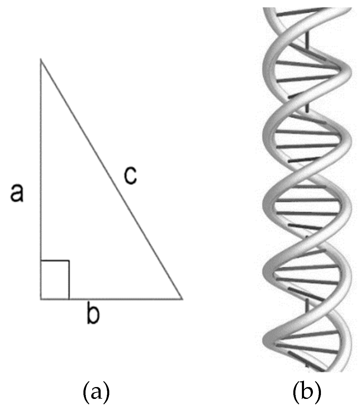
Figure 1.
Double helix of lines sa and sb.
Figure 2.
Illustration of a 4 line spiral
Such a spiral will be called a 4-braid (i.e., a bundle consisting of 4 interlaced lines ), wherein:
- -
- the line belongs to the outer side of the a-th affine space;
- -
- the line belongs to the inner side of the a-th affine space;
- -
- the line belongs to the outside of the b-th affine space;
- -
- the line belongs to the inner side of the b-th affine space.
The addition of quadratic forms (29) or their averaging (29a) depends on the model representation. If we assume that two metric spaces are additively superimposed on each other, then the addition operation (29) should be used. If we assume that a metric space can be in a state with the metric sa2 or with the metric sb2 with equal probability, then this corresponds to the quantum mechanical approach, and the averaging operation (29a) should be used.
At this stage of the study, it is difficult to decide which operation "addition" (29) or "averaging" (29a) should be used. However, the quantum mechanical approach provides additional opportunities for probability theory and does not require an answer to the question: "Is the sum of solutions (for example, sa2 and sb2) of Einstein's non-linear differential equations also a solution of this equations?". Therefore, the quantum mechanical approach looks much more preferable, especially when the sum of solutions is also a solution to a nonlinear equation. Arguments in favor of the second approach are presented in Appendix 1, see Ex.s (4.A1) – (32.A1).
Now, for example, consider the averaging of four metrics (14) – (20)
dS1-4 = 1/4(ds1(–)2+ ds2(–)2 +ds3(–)2+ ds4(–)2).
As a result, we obtain the averaged metric
By analogy with (29) – (30), such a metric space is based on the interweaving of four affine extensions, which respectively belong to 8 linear forms dsi(–) and dsi(–)′, i.e. segments of 8 lines twisted into an 8-braid.
Such an 8-braid is described by a system of two complex conjugate quaternions:
whose product is equal to the metric (32).
On Figure 3 shows an illustration of the interweaving of several affine subspaces that form a multilayer metric space.
Properties of intertwined affine subspaces and multilayer metric spaces with signatures (+ – – –) and (– + + +) corresponding to the “vacuum balance” condition
detailed in the "Algebra of signatures" [16,17].
(+ – – –) + (– + + +) = 0
In the same papers [16,17], a more detailed analysis was carried out, considering metric spaces with all sixteen possible signatures:
which in total correspond to the principle of "full vacuum (i.e., zero) balance", (37a)
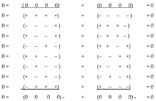 |
In this expression, called in [16,17] ranking, the summation of the signs "+" and "–" is performed both in columns and in rows.
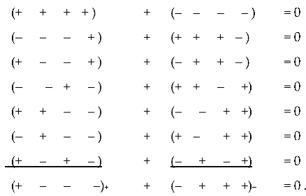 |
(37b)
That is, the additive superposition (in this case, the addition of signs of signatures by columns) of seven metric spaces with signatures in the denominator of the left column of the ranking Ex. (37b), form a Minkowski space with signature (+ – – –).
Whereas the additive superposition of seven metric spaces with signatures in the denominator of the right column of the ranking Ex. (37b), form an anti-Minkowski space with the opposite signature (– + + +).
3. Extended Einstein's field equations
In the previous paragraphs of this article, we considered a set of solutions to the Einstein field equations (8), well known to specialists. In this paragraph, for the first time, it is proposed to consider an extended version of this equations.
Recall that Einstein, in order to write Eq.s (3), used the following property of the metric tensor
however, it is obvious that the covariant derivative of the infinite series is also equal to zero
where Λ1, Λ2, … , Λ∞ are constants that can take both positive (Λi > 0) and negative (Λi < 0) values.
Therefore, we use the same method that Einstein used to introduce the Λ-term into Eq.s (1) [2], and write the equations
or in a more compact form
where Λj = 3/rаj2 or – 3/rаj2, here raj is the radius of the j-th spherical formation.
If the sum of the series Λ1 + Λ2 + Λ3 +…+ Λ∞ converges to a constant number Λ0, i.e., if
then Eq.s (40) takes the form of Eq.s (5)
which, like (6) – (7), is reduced to the form similar to Eq.s (8)
Therefore, the solutions of Eq.s (43) practically coincide with the solutions (14) – (25):
- with signature (+ – – –)
- and with signature (– + + +)
where and are the zero results of the summation of alternating series
where Nj are the dimensionless corrective parameters of the considered cosmological model.
Such a cosmological model is the most optimal, since in the case of (54) the extended Einstein field equations as a whole take on the simplest form
with four Schwarzschild solutions
which, when condition (55) is met, turn into two Minkowski solutions (20) and (25), which is consistent with the principle of “maximum rationality” and the principle of “total average absence” (i.e., observance of the “vacuum balance”).
At the same time, it is possible that there is a slight imbalance between the positive and negative members of the series (54)
where j =1,2,3,…
For example, it is possible that the imbalance exists, but is extremely small.
i.e., tend to the value published by the Plank collaboration [14] for the Standard cosmological model Lambda-CDM; where is the total cosmological constant (TCC).
Then Eq.s (43) takes the form
with four de Sitter solutions
In this case, according to Ex.s (7) and (4)
If there is a predominance of positive terms in Ex. (55b), then > 0 (de Sitter universe); if negative terms predominate, then < 0 (anti - de Sitter universe).
At the same time, in the author's opinion, the "vacuum balance" cannot be violated, since only mutually opposite entities can appear from the void (for example, convexity - concavity, wave - antiwave, particle-antiparticle, etc.). Therefore, if an imbalance (55b) of type > 0 exists, then a counter-imbalance of type < 0 must also coexist.
It is possible to restore the averaged “vacuum balance” in such a situation if we assume that the sign of the total cosmological constant (TCC) periodically changes with time. For example, it can be assumed that the value of the TCC fluctuates according to a sinusoidal law with an amplitude . Then, on average, the “vacuum balance” is restored
where is the cosmological oscillation frequency.
4. Closed ten-layer and ten-level cosmological model
In the previous section, it was shown that the extended Einstein field equations can contain an infinite number of -terms, provided that the sum of all these terms must tend to zero to maintain the “vacuum balance”.
Further, it will be shown that the cosmological model based on the extended Einstein field equations (43), taking into account Ex.s (54) and (55) [or (55b) and (55c)], can be a closed spherical space filled with an infinite number of spherical formations ("bubbles") and opposite anti-spherical formations ("anti-bubbles") with different radii , inside which there is an infinite number of smaller "bubbles" and "anti-bubbles" with different radii , and so it continues to infinity from level to level (see Figure 4).
At this point, for simplicity, we single out only ten levels with two mutually opposite spherical formations (i.e., a “bubble” and an “anti-bubble”) at each level.
In other words, to identify the main parameters of the multilevel cosmological model, we study a special case when, instead of infinite series (54) and (55), we use a simplified series limited by ten mutually opposite pairs of terms:
Consider separately the series with positive and negative terms
Let’s substitute series (58) into metrics (44) – (48) instead of series (56) and (57) and take into account that we can write:
As a result, we obtain five metrics with signature (+ – – –):
Similarly, substitution of series (59) into metrics (49) – (53) leads to the following five similar metrics, but with the opposite signature (– + + +):
Let's try to connect the radii rj, included in Ex.s (56) and (57), with the characteristic sizes of bodies in the world around us.
Let's assume that in the basis of a fully geometrized cosmological model there are only two geometric constants: Rv is the parametric radius of the universe, and lс ≈ сΔt ≈ с·1sec ≈ 2.9·1010 cm is the distance that a light beam travels in vacuum in a time interval Δt = 1 sec.
Let’s assume that the radii rj in the metrics (64) – (73) are estimated by the recursive formula consisting of the above two constants
where cm is the distance obtained by raising the number 2.9·1010 to the power j (1, 2,…,10) with the dimension centimeter.
rj ~ Rv2/lсj,
If we assume Rv ≈ 1025 cm, then we obtain the following approximate recurrent formula
from which follows a hierarchical sequence of radii of ten spheres nested into each other (see Figure 5 and Figure 6):
(76)
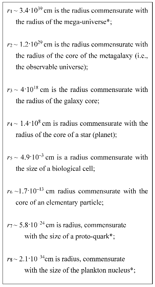 |
Figure 5.
Hierarchical sequence of nested spherical formations.
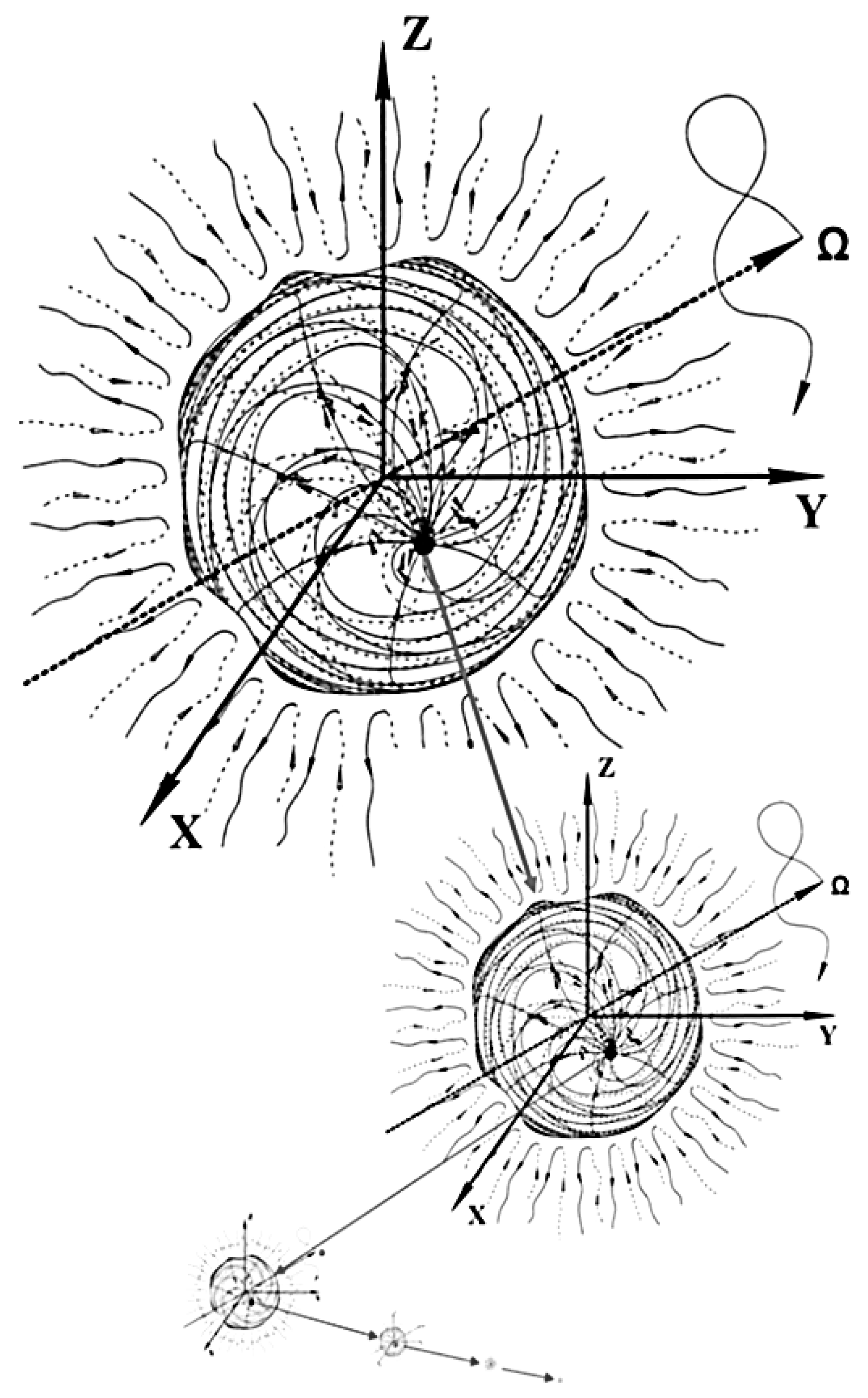
Figure 6.
Three levels of a sequence of nested spherical formations.
The existence of spherical formations marked with an asterisk * has not been confirmed in practice due to the imperfection of modern technology. Therefore, it is proposed to consider the 10-level cosmological model as a speculative forecast of the author intended for the first working hypothesis. This forecast is based on the confessional intuition of the author, connected with the philosophical doctrine of the “Tree of Life” (i.e., “Tree of ten Sefirot”).
However, the radii r2, r3, r4, r5 and r6 from the sequence (76), obtained using the recurrent formula (75), surprisingly turned out to be commensurate with the characteristic sizes of the cores (or nuclei) of the observed discrete hierarchical sequence of real spherical formations: metagalaxies, galaxies, stars (planets) and biological cells, while the radius r6 practically coincided with the "classical radius of the electron" 2.8·10–13 cm. Therefore, it is possible that compact formations with characteristic sizes r1, r7, r8, r9 and r10 can also be detected over time.
Metrics (64) – (73) with a hierarchical sequence of radii rj (76) describe the metric-dynamic state of a sequence of ten nested multilayer spherical formations (see Figure 5 and Figure 6), the proportions of which partially coincide with the sizes of a discrete sequence of cores (or nuclei) of real objects [17]. Therefore, such a ten-layer and ten-level cosmological model looks promising for further development and refinement.
However, this hierarchical model has one circumstance that does not lend itself to logical understanding. The fact is that from metrics (64) – (73) it follows that the 1-st sphere (whose radius is commensurate with the radius of the mega-universe r1 ~ 1039 cm) is located inside the 10-th sphere (with the instanton size r10 ~ 10–55 cm).
To verify this, follow, for example, the sequence of terms:
and pay attention to the last term, which contains r1 and r10. This means that the sphere with radius r1 is inside the sphere with radius r10 [17], as can be seen from the previous terms of the same expression. A similar situation takes place in all metrics (64) – (73).
Such isolation of the proposed 10-layer and 10-level cosmological model looks very extravagant and requires additional study and reflection. However, the history of science teaches that sometimes what looks impossible is disproved by experiment. For example, 100 years ago, Einstein and many of his contemporaries could not admit the idea that the part of the universe we observe is expanding with acceleration.
Note that today we do not see only the upper and lower "ends" of the proposed 10-layer and 10-level cosmological model, but in the interval from r2 ~ 1028 cm (scale of the observable universe) to r6 ~ 10–16 cm (intranuclear scale), this model can be useful for solving many problems.
5. Metric-dynamic models of «electron» and «positron»
For example, let’s select from a hierarchical discrete sequence of spheres nested into each other (see Figure 5 and Figure 6) two mutually opposite spherical formations with a radius r6 ~ 10–13 cm, which corresponds to the characteristic size of the "core" of an elementary particle (in particular core of the «electron» and "positron"). All other spherical formations from the considered hierarchical model (64) – (73) are arranged similarly.
In this work, the names of the particles are quoted, for example, «electron», since the metric-dynamic models of these spherical formations differ in many respects from the model ideas about these formations in modern physics.
In metrics (64) – (68), let’s leave for consideration only those terms that contain radii r6. As a result, we obtain the following multilayer metric-dynamic model of a "convex" spherical formation, which we will call «electron»:
where r5 ~ 10–3 cm, r6 ~10–13 cm, r7 ~10–24 cm.
«ELECTRON»
"Convex" multilayer spherical formation with
a signature (+ – – –), consisting of:
The outer shell of the «electron»
in the interval [r5, r6] (Figure 7)
The сore of the «electron»
in the interval [r5, r6] (Figure 7)
The shelt of the «electron»
in the interval [0, ∞]
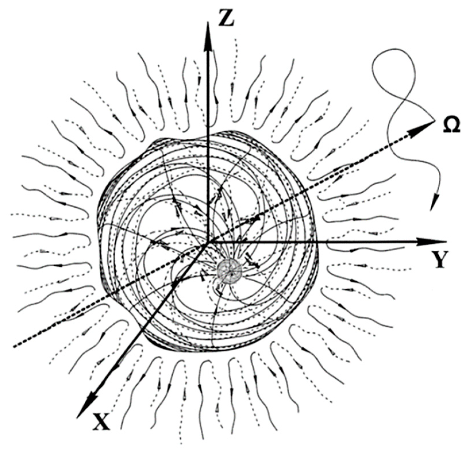
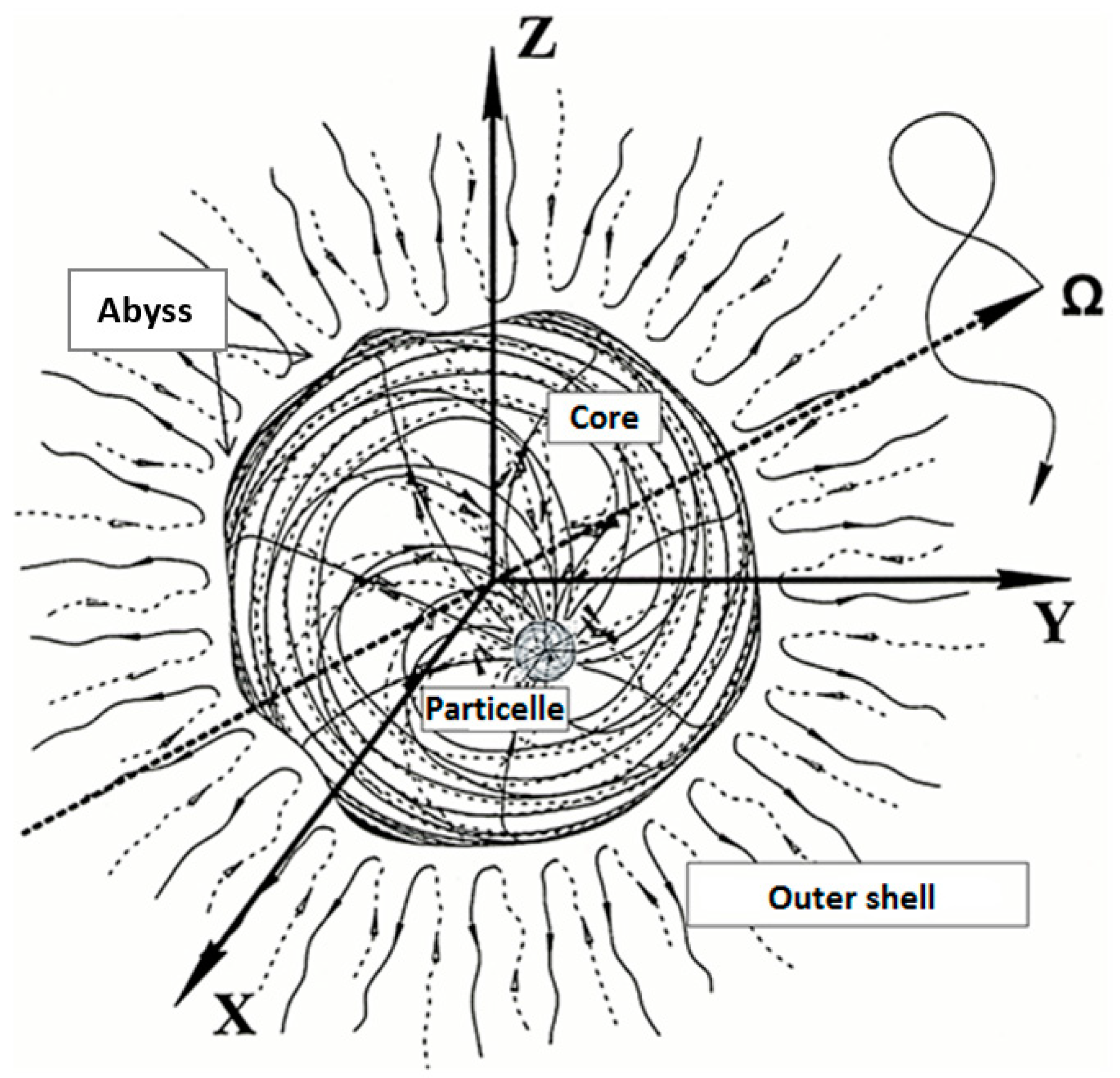
Figure 7.
A model of a spherical formation (in particular, an «electron») with four clearly defined areas: "outer shell", "abyss" (or "rakia"), "core" and inner "nucleolus" (or “particelle”).
Figure 7.
A model of a spherical formation (in particular, an «electron») with four clearly defined areas: "outer shell", "abyss" (or "rakia"), "core" and inner "nucleolus" (or “particelle”).
Similarly, in the metrics (69) – (73) we also leave only those terms that contain the radii r6. As a result, we obtain the following multilayer metric-dynamic model of a "concave" spherical formation, which we will call «positron»:
where r5 ~ 10–3 cm, r6 ~10–13 cm, r7 ~10–24 cm.
«POSITRON»
"Concave" multilayer spherical formation with
a signature (– + + +), consisting of:
The outer shell of the «positron»
in the interval [r5, r6] (negative of the Figure 7)
The core of the «positron»
in the interval [r5, r6] (negative of the Figure 7)
The shelt of the «positron»
in the interval [0, ∞]
The sets of metrics (78) and (88) differ only in their signature. That is, «electron» and «positron» are completely identical, but antipodal copies of each other. If an «electron» is conventionally called a "convex" spherical formation, then a «positron» is exactly the same conventionally "concave" spherical formation.
The Figure 7 shows a metric-dynamic (i.e., fully geometrized) model of a spherical formation with a radius from the hierarchical sequence (76). In a particular case, an «electron» (and/or its exact antipodal copy, a "positron") has (see Figure 7):
- -
- core with radius r6 ~10–13 cm;
- -
- inner “nucleolus” with radius r7 ~10–24 cm;
- -
- "outer shell", extending from r6 ~10–13 cm to r5 ~ 10–3 cm (or up to r4 ~ 108 cm, or up to
r3 ~ 1018 cm and etc. depending on which spherical formation the given core of the «electron» is located inside).
In another case, for example, «planets» (or «anti-planets»): the "core" has a radius r4 ~1,4·108 cm; the inner "nucleolus" has a radius r5 ~ 10–3 cm (or r6 ~ 10-13 cm, etc., depending on which spherical formation is located inside the core of the «planet»), and "outer shell" extends from r4 ~ 108 cm to r3 ~ 1018 cm (or up to r2 ~ 1029 cm, or up to r1 ~ 1039 cm and depending on, inside which sphere is the core of the "planet"). And so on.
The "shelt" (87) or (97) of a spherical formation begins at its center, and ends at infinity. The "shelt" is a kind of memory of the undeformed state of the considered area of space. The “shelt” does not seem to exist in the curved state of this area of space, but without the components of the metric tensor of the "shelt" or it is impossible to determine the deformation, relative elongation, speed and direction of movement of each local section of the object under study (see [16,17]).
The "abyss" (or "rakia") (see Figures 7) is a spherical boundary between the "core" and the "outer shell" of any spherical vacuum formation. The "rakia" is the most complex spherical area of the object under study, since it contains sub-layers associated with all higher spheres, inside which is the core of the «electron» (see Figures 5), as well as sub-layers associated with all the spheres that are inside the same core of the «electron».
A detailed study of the sets of metrics (79) – (87) describing the «electron» and (89) – (97) describing the «positron» is given in [17]. In the same place, taking into account all sixteen signatures (37), metric-dynamic models of almost all elementary particles included in the Standard Model are proposed: all types of «quarks», all types of «neutrinos», «mesons», etc., with the exception of Higgs boson (see Appendix 2 and also http://metraphysics.ru Contents, Chapter 2, sections 2.9 – 2.14).
6. Conclusion and discussion
The article proposes to take into account all 10 Kottler solutions (14) – (25) of the system of Einstein field (vacuum) equations (9) when constructing a multilayer and multilevel cosmological model, balanced on average with respect to the Einstein vacuum (i.e., "emptiness").
It is shown that the averaging of metric spaces represented by the quadratic forms and (14) – (25) is connected with the intertwining (i.e. twisting into bundles or braids) of the corresponding affine spaces, represented by linear forms and . Moreover, these affine bundles are described by Clifford algebras with the number of generators equal to the number of intertwined linear forms and (see [16,17]).
The second innovation proposed in this article is related to the increase to infinity of Λi-terms in Einstein's field equations (1).
The restrictions imposed on the sum of Λi-terms made it possible to propose a 10-layered and 10-level (hierarchical) cosmological model.
This model is a hierarchical sequence of nested spheres (see Figure 5) with the corresponding radii ri (76), which are obtained using the recurrent formula (75) using only two dimensional parameters: Rv ≈ 1025 cm is parametric the radius of the universe, and lс ≈ 2,9·1010 cm is the distance that a light beam travels in vacuum in a single time interval Δt = 1sec.
Wherein, part of the radii r2, r3, r4, r5 and r6 from the hierarchy (76) turned out to be commensurate with the characteristic sizes of the core (or nuclei) of the observed discrete sequence of real spherical formations (i.e., cores): metagalaxies, galaxies, stars (planets), biological cells (bacteria) and elementary particles.
At the end of the article, from the hierarchical solutions (64) – (73), the metric-dynamic models of the «electron» (78) and «positron» (88) are singled out, which are part of the proposed ten-layer and ten-level cosmological model.
Similarly, from solutions (64) – (73) can be singled out metric-dynamic models a «biological cell» with characteristic radius r5 ~ 10–3 cm, a «star» with characteristic core radius r4 ~ 108 cm and a «galaxy» with characteristic core radius r3 ~ 1018 cm, etc.
Mathematical techniques that allow extracting various information about local spherical formations from a set of the solutions of extended Einstein's field equations, including a geometrized description of all particles that included in the Standard Model and all known force interactions: electrostatic, electromagnetic, weak and nuclear, are presented in the author's work [17] and on the website www.metraphysics.ru.
The advantages of the multilayer and multilevel cosmological model, proposed in this article, include:
- the complete absence of the need to introduce the concept of matter and its energy-momentum tensor as a source of curvature of 4-dimensional space. Here matter is replaced by an infinite number of spherical objects (see Figure 5 and Figure 6) with 10 types of characteristic sizes rj (76) [17]. In this case, the right side of the Einstein-Hilbert equations (1) naturally vanishes. In this case, Einstein's field equations (8) and (43) are the general covariant expression of the conservation laws [16,17].
The disadvantages of the hierarchical 10-layer and 10-level cosmological model proposed in this article include:
- causal and logical inconsistency of this type of closedness of the universe, in which the largest sphere with the size r1 ~ 1039 cm is inside the smallest sphere with the size r10 ~ 10–55 cm, see, for example, Ex. (77a);
- unreasonable presence of the anthropic principle element in the recurrent formula (75), since the distance lс ≈ с·1sec ≈ 2,9·1010 cm, which passes a light beam in vacuum in 1 sec (i.e., approximately during the period of oscillation of the human heart);
- an intuitive (i.e., scientifically unfounded) choice of 10 levels (nested spheres) of the cosmological model, despite the fact that today only five discrete levels out of ten are observed.
- the model does not answer the question why we observe a discrete (i.e., in fact, quantum) scale hierarchy of spherical formations (galaxies, stars, biological cells, elementary particles, etc.). The proposed model only "copies" such a discrete-hierarchical manifestation of reality. Obviously, Einstein's field equations (8) and (43) do not contain the possibility of explaining hierarchical discretization (i.e., scaling quantization). This means that Einstein's field equations are not complete. Perhaps, the Einstein-Cartan equations with torsion, or the equations of the geometry of absolute parallelism in a tetrad representation, have such properties. On the other hand, it can be assumed that hierarchical discreteness is not the result of the properties of differential equations, but is associated with boundary conditions. This is how Maxwell's equations for a waveguide or resonator lead to a discrete spectrum of electromagnetic waves.
At the same time, the multilayer and multilevel cosmological model proposed here is variable, that is, it can be refined as further analysis and accumulation of empirical data.
Acknowledgements
For assistance, I express my deep appreciation and gratitude to the mathematician David Reid (USA, Israel), Ph.D. Tatyana Levi, IT-specialist Alexander Maslov and Eliezer Reichman.
Appendix 1
The first Einstein field equation and its solutions
The Einstein-Hilbert equation for empty space (i.e., Einstein vacuum) has the form of equation (1) for
where is the scalar curvature;
is Ricci tensor;
is Christoffel symbols.
Combining Eq.s (1.A1) with the contravariant components of the metric tensor , we obtain
where is the number of space dimensions.
For any n-dimensional space (except for n = 2), equality (2.A1) can be satisfied only for R = 0. Therefore, for n = 4, Eq. (1.A1) takes the simplest form
We will call this equation the first Einstein vacuum equation, and it is an expression of the conservation laws, since
In this case, the solutions of Eq.s (3.A1) describe the metric-dynamic state of stable vacuum formations.
Einstein wrote [19]: “The equation of gravity for empty space is the only rationally substantiated case of field theory that can claim to be rigorous.”
Solutions of the Eq.s (3.A1) are considered in many works on modern differential geometry and general relativity. However, none of the publications known to the author discusses the relationship between various solutions of this equations, so we will consider it in sufficient detail.
Solutions to Eq.s (3.A1) are sought in a spherical coordinate system in the form of metrics:
where ν and λ are the required functions of t and r.
ds(–)2 = еνс2dt2 – еλdr2 – r2dθ 2 – r2sin2θ dϕ 2 with signature (+ – – –),
ds(+)2 = –еνс2dt2 + еλdr2 + r2dθ 2 + r2 sin2θ dϕ 2 with signature (– + + +),
As a result of substitution of the covariant and contravariant components of the metric tensor from the metric (4.A1) into Eq. (3.A1) for the stationary (i.e., time-independent) state of the "vacuum", a system of three equations is obtained [20]:
ν = – λ ,
– е ν (ν′ /r + 1/r2) + 1/r2 = 0,
ν′′ + ν′ 2 + 2ν′ /r = 0.
The differential Eq. (7.A1) has three solutions:
where h1, h2, h3 are integration constants.
ν1 = ln(h1+ h2 /r), ν 2 = ln(h1 – h2 /r), ν3 = h3,
Eq. (8.A1) also has three solutions:
where rb is the integration constant (the radius of the spherical volume).
ν1 = ln(1+ rb b/r), ν 2 = ln(1 – rb /r), ν 3 = 0,
For h1 = 1, h2 = rb and h3 = 0, the solutions of Eq.s (7.A1) and (8.A1) coincide.
Substituting three possible solutions (10.A1) into the metric (4.A1) we get three metrics with the same signature (+ – – –):
ds1(–)2 = (1– rb /r)с2dt2 – (1– rb /r) –1dr2 – r2dθ 2 – r2sin2θ dϕ 2,
ds2(–)2 = (1+ rb /r)с2dt2 – (1+ rb /r) –1dr2 – r2dθ 2 – r2sin2θ dϕ 2,
ds3(–)2 = с2dt2 – dr2 – r2dθ 2 – r2sin2θ dϕ 2.
Performing similar operations with the components of the metric tensor from the metric (5.A1), we obtain three more metrics that also satisfy Eq.s (3.A1), but with the opposite signature (– + + +):
ds1(+)2 = – (1– rb /r)с2dt2 + (1– rb /r) –1dr2 + r2dθ 2 + r2sin2θ dϕ 2,
ds2(+)2 = – (1+ rb/r)с2dt2 + (1+ rb /r) –1dr2 + r2dθ 2 + r2sin2θ dϕ 2,
ds3(+)2 = – с2dt2 + dr2 + r2dθ 2 + r2sin2θ dϕ 2.
Irreducible into each other metrics (11.A1) – (16.A1) will be called generalized Schwarzschild metrics.
Metrics (11.A1) – (16.A1) describe the metric-dynamic state of the same vacuum region, therefore it is proposed to consider various options for averaging them, despite the fact that Eq.s (3.A1) is non-linear and, as a rule, in such cases, the sum of his decisions is not his own decision.
If the centers of the metrics (11.A1) – (13.A1) and (14.A1) – (16.A1) are aligned, then it is obvious that their sum is equal to zero
is also a trivial solution of the vacuum Eq.s (3.A1).
ds1(–)2+ds2(–)2+ds3(–)2+ds1(+)2+ds2(+)2+ds3(+)2 = 0∙с2dt2 +0∙dr2 + 0∙dθ 2+ 0∙sin2θ dϕ 2= 0.
Received metric ds(0)2 = gij(0) dxi dxj ,
Thus, contrary to expectations, the addition of six metrics (11.A1) – (16.A1) led to an additional solution to Eq. (3.A1).
Consider now the arithmetic mean of two metrics (11.A1) and (12.A1)
The distance between two points r1 and r2 along the length with the signature (+ – – –) in general relativity is determined by the expression
in the case of substitution from the averaged metric (20.A1), we obtain
Let’s first find the value of the segment between the points r1= rb and r2 = ∞:
The length of this segment is equal to the radius of the cavity rb, and the imaginary nature of this result indicates that there is no "vacuum" in the cavity. Outside this cavity from r1= rb to r2 = ∞ we have
In the absence of vacuum deformation, the distance between the points r2 = ∞ and r1 = rb is equal ∞ – rb, and in the case under consideration it is equal to (24.A1). The difference between these segments is approximately equal to
This result shows that the average vacuum extension on the segment ]rb, ∞[ is compressed by the value ~ rb, in all radial directions due to the fact that it is displaced from the cavity with radius (25.A1). This result is similar to an air bubble in a liquid (Figure 2.A.1).
The difference between the initial (non-curved) state of a local area of vacuum and its actual (curved) state is determined by the difference [21]
Figure 2.A1.
Air bubble in liquid
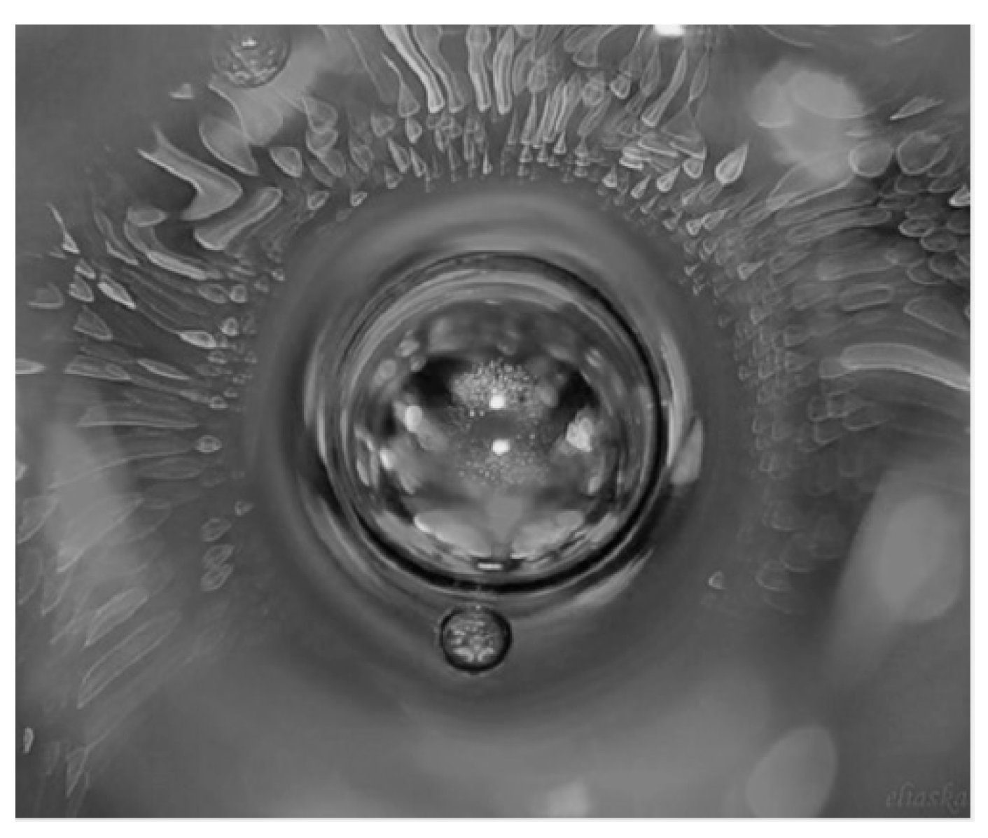
Figure 3.A1.
Graph of the function lr(–) – the relative elongation of the vacuum in the outer shell surrounding the spherical cavity. The calculation was performed at rb = 2, using the software MathCad 15
Figure 3.A1.
Graph of the function lr(–) – the relative elongation of the vacuum in the outer shell surrounding the spherical cavity. The calculation was performed at rb = 2, using the software MathCad 15
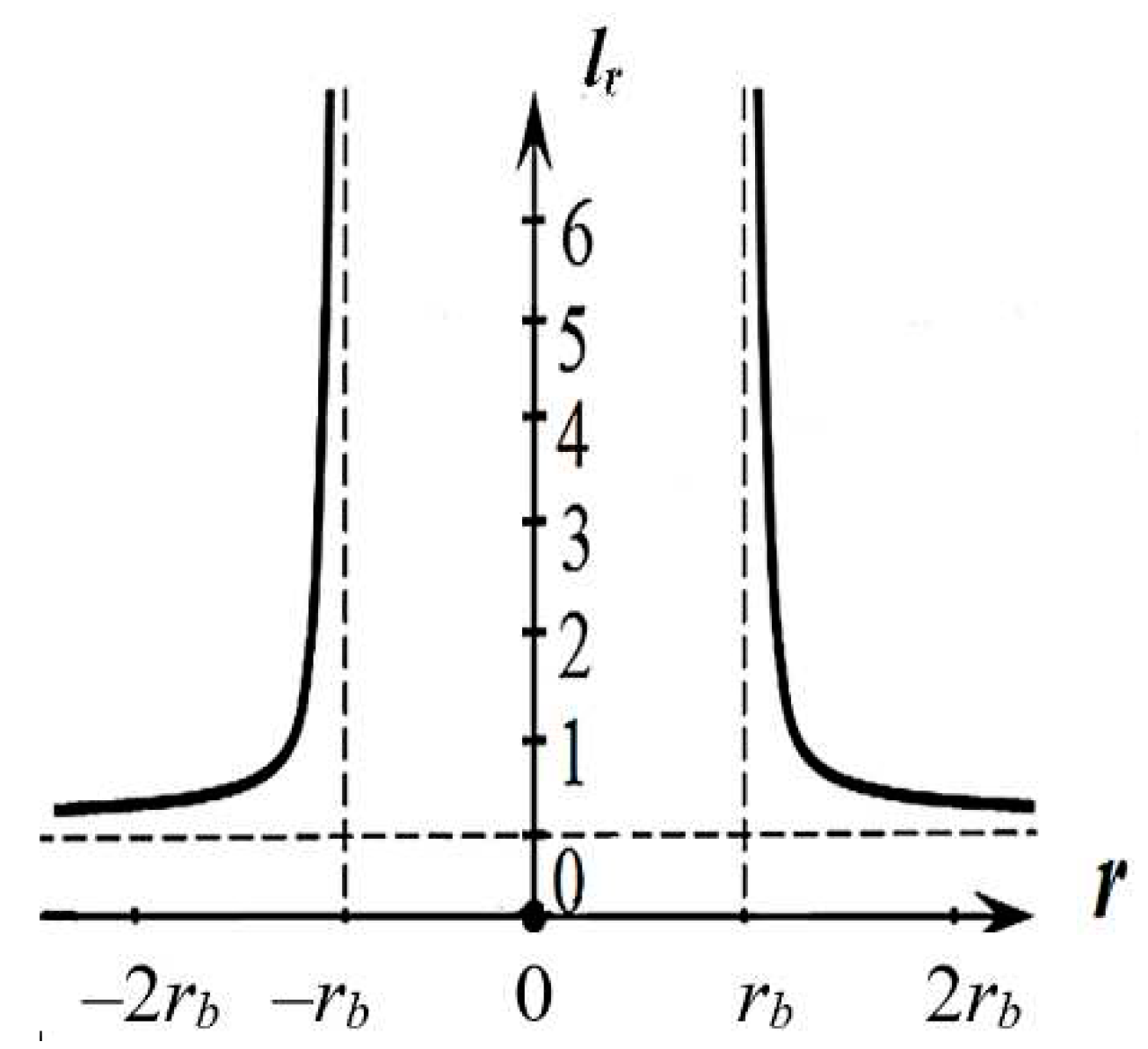
The relative elongation of the vacuum region in this case is [21]
ds(–)2 = (1 + l(–))2 ds0(–)2,
The uncarved state of the vacuum section under consideration is given by the metric (13.A1), therefore, substituting the components gii0(–) and gii(–), respectively, from (13.A1) and (20.A1) into (29.A1), we obtain the relative elongation of the vacuum in each radial direction in the region from rb to ∞ (30.A1)
The graph of the function lr(–) (30.A1) is shown in Figure 3.A1. For r = rb, this function tends to infinity, and for r < rb it becomes imaginary.
Here we will not discuss the question: – What is inside the cavity with radius rb, if the vacuum is displaced from there? When considering the second and third Einstein vacuum equations (8) and (43), this problem will be solved by itself.
Thus, averaging the metrics (11.A1) and (11.A1) leads to a metric-dynamic description of a stable vacuum formation of the "air bubble in liquid" (see Figure 3.A1) type, while these metrics alone do not lead to such results.
Averaging the metrics (14.A1) and (15.A1) allows you to get similar results, but with the opposite signature
Appendix 2
The Standard Model of Elementary Particles
from the Algebra of signatures
1.A2 Models of хi+-«quark» and xi–-«antiquark» in the Algebra of signatures
The fundamentals of "Algebra of signatures" and "Stochastic Metraphysics" (that is, fully geometrized physics from the standpoint of Algebra of signatures) are described in [16,17].
This Appendix contains only the main conclusions of the Algebra of signatures related to the Standard Model of elementary particles (Figure 1.A2).
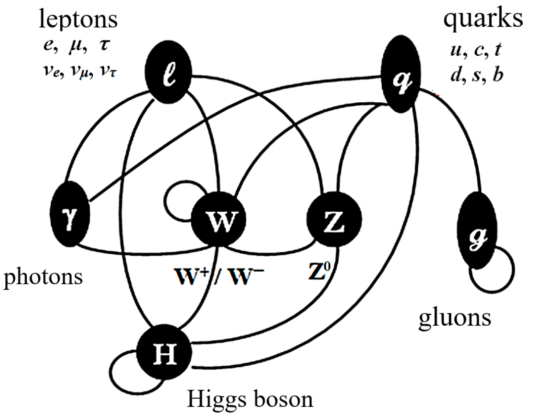
Figure 1.A2.
Elements of the Standard Model of elementary particles
In the above article, it was conditionally assumed that an «electron» is a spherical convexity in empty space (i.e., the Einstein vacuum), which is described by a set of metrics (79) – (87) with the signature (+ – – –); and a «positron» is the exact opposite copy of an «electron», i.e. spherical concavity in the Einstein vacuum, which is described by a set of metrics (89) – (97) with an inverted signature (– + + +).
The Algebra of signatures takes into account all 16 signatures (37), and the "building material" of the entire variety of observed objects are «quarks» and «antiquarks»:
Хi–-«QUARK» or Хi+-«ANTIQUARK»
"Convex-concave" multilayer spherical formation
with one of the following signatures:
The outer shell of thexi+-«quark» orxi–-«antiquark»
in the interval [r5, r6] (Figure 8)
The core of thexi+-«quark» orxi–-«antiquark»
in the interval [r6, r7] (Figure 8)
The shelt of thexi+-«quark» orxi–-«antiquark»
in the interval [0, ∞]
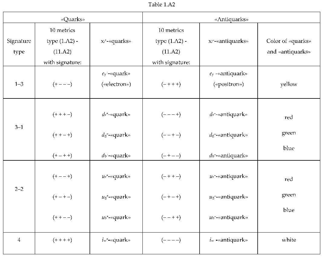
Signatures, colors and names of all 16 possible xi+-«quarks» and xi–-«antiquarks» presented in Table. 1.A2.
Note that within the framework of the Algebra of signatures, these 16 xi+-«quarks» and xi–-«antiquarks» refer not only to elementary particles, but also to any other spherical formations from the hierarchy (76). Only instead of radii r5 , r6 , r7 in metrics (1.П2) – (11.П2) it is necessary to substitute accordingly: for bacteria r4 , r5 , r6; for stars r3 , r4 , r5; for galaxies r2 , r3 , r4 etc.
 |
For example, let's represent a ur–-«antiquark» in expanded form:
where r5 ~ 10–3 cm, r6 ~10–13 cm, r7 ~10–24 cm.
ur–-«ANTIQUARK»
"Convex-concave" multilayer spherical formation
with the signatures (– + + –), consisting of:
The outer shell of theur–-«antiquark»
in the interval [r5, r6] (Figure 8)
The core of the ur–-«antiquark»
in the interval [r6, r7] (Figure 8)
The shelt of the ur–-«antiquark»
in the interval [0, ∞]
Let's introduce the notation for 16 types of spherical formations: (22.A2)
10* metrics of the form (12.A2) with signature (+ – – –) – yellow ey–-«quark» («electron»);
10 metrics of the form (12.A2) with signature (– + + +) – yellow ey+-«antiquark» («positron»);
10 metrics of the form (12.A2) with signature (+ + + –) – red dr+-«antiquark»;
10 metrics of the form (12.A2) with signature (+ + – +) – green dg+-«antiquark»;
10 metrics of the form (12.A2) with signature (+ – + +) – blue db+-«antiquark»;
10 metrics of the form (12.A2) with signature (– – – +) – red dr–-«quark»;
10 metrics of the form (12.A2) with signature (– – + –) – green dg–-«quark»;
10 metrics of the form (12.A2) with signature (– + – –) – blue db–-«quark»;
10 metrics of the form (12.A2) with signature (+ – – +) – red ur+-«antiquark»;
10 metrics of the form (12.A2) with signature (+ – + –) – green ug+-«antiquark»;
10 metrics of the form (12.A2) with signature (+ + – –) – blue ub+-«antiquark»;
10 metrics of the form (12.A2) with signature (– + + –) – red ur–-«quark»;
10 metrics of the form (12.A2) with signature (– + – +) – green ug–-«quark»;
10 metrics of the form (12.A2) with signature (– – + +) – blue ub–-«quark»;
10 metrics of the form (12.A2) with signature (– – – –) – white iw–-«quark»;
10 metrics of the form (12.A2) with signature (+ + + +) – white iw+-«antiquark».
*10 metrics (12.A2), because Shelt type (21.A2) refers to both the "core" and the "outer shell" of the corresponding xi–-«quark» or xi+-«antiquark» (Figure 8). Thus, 5 metrics describe the "core", and 5 metrics describe the "outer shell" of each xi–-«quark» and xi+-«antiquark».
Of the spherical formations (22.A2), only a convex formation are stable – «electron» (ey–-«quark») with the signature (+ – – –) and a concave formation is a “positron” (ey+-«antiquark») with signature (– + + +), because they consist of solutions of Einstein's field equations (8), which is the stability condition. All other spherical formations from the list (22.A2) are unstable, because do not satisfy the conditions of stability (8). That is, when substituting the components of metric tensors from metrics (1.A2) – (11.A2) with any other signature except (+ – – –) and (– + + +) into Eq.s (8), equality will not work.
At the same time, out of 16 xi+-«quark» and xi–-«antiquark» from the list (22.A2) it is possible to compose averaged stable spherical formations with signatures (+ – – –) or (– + + +). This will be shown in the following paragraphs.
2.A2 Models of «proton» and «antiproton» in the Algebra of signatures
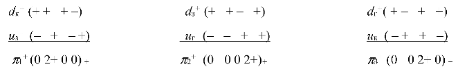
On average, stable spherical formations with signatures (+ – – –) or (– + + +) can be composed of two different-colored u-«quarks» (or u-«antiquarks») and one d-«quark» (or d-«antiquark») from the list (22.A2):
where pi– are three possible states of pi–-«proton» (i = 1, 2, 3) with signature (– + + +)
where pi+ are three possible states of pi+-«antiproton» with signature (+ – – –).
 |
 |
In a more compact form, the states a pi–-«proton» and pi+-«antiproton» can be represented as
p1+ = uз–uг–dк+, p2 + = uк– uг– dз+, p3+ = uз– uк– dг+,
p1– = uз–uг–dк+, p2 – = uк– uг– dз+, p3– = uз– uк– dг+.
This type of recording of the states of the «proton» and «antiproton» almost completely coincides with the recording of the states of the proton and antiproton in modern quantum chromodynamics, on which the Standard Model of elementary particles is based.
The difference, however, is that in the Standard Model, protons are made up of quarks and antiprotons are made up of antiquarks, while in the Algebra of signatures pi–-«proton» and pi+-«antiproton» are made up of xi+-«quarks» and xi–-«antiquarks». Therefore, in the Algebra of signatures, there is no problem associated with the baryon asymmetry of the Universe.
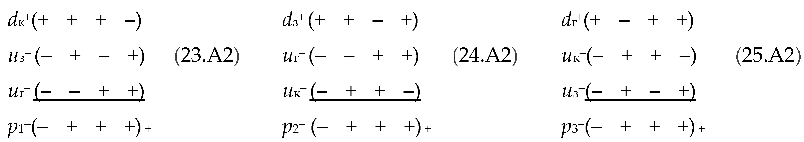
For example, let's imagine a multilayer metric-dynamic model of pi–-«proton» (23.A2)
in the expanded form:
dк+(+ + + –)
uз– (– + – +)
uг–(– – + +)
р1+(– + + +) +
p1–-«PROTON»
On average, a "concave" multilayer vacuum formation
with a common signature (– + + +)
consisting of:
dr+-«quark»
"Convex-concave" multilayer spherical formation
with the signatures (+ + + –), consisting of:
The outer shell of the dr+-«quark» (+ + + –)
in the interval [r5, r6] (Figure 1.A2)
The core of the dr+-«quark» (+ + + –)
in the interval [r6, r7] (Figure 1.A2)
The shelt of thedr+-«quark» (+ + + –)
in the interval [0, ∞]
ug–-«antiquark»
"Convex-concave" multilayer spherical formation
with the signatures (– + – +), consisting of:
The outer shell of the ug–-«antiquark» (– + – +)
in the interval [r5, r6] (Figure 1.A2)
The core of the ug–-«antiquark» (– + – +)
in the interval [r6, r7] (Figure 1.A2)
The shelt of the ug–-«antiquark» (– + – +)
in the interval [0, ∞]
ub–-«antiquark»
"Convex-concave" multilayer spherical formation
with the signatures (– – + +), consisting of:
The outer shell of the ub–-«antiquark» (– – + +)
in the interval [r5, r6] (Figure 1.A2)
The core of the ub–-«antiquark» (– – + +)
in the interval [r6, r7] (Figure 1.A2)
The shelt of the ug–-«antiquark» (– – + +)
in the interval [0, ∞]
Figure 1.A2.
Core of the «proton» consists of 3 practically superimposed cores: the core of one d-«quark» and of two cores u-«antiquarks». The inner nucleoli of these 3 "quarks" are in constant chaotic movement and interweaving with each other.
Figure 1.A2.
Core of the «proton» consists of 3 practically superimposed cores: the core of one d-«quark» and of two cores u-«antiquarks». The inner nucleoli of these 3 "quarks" are in constant chaotic movement and interweaving with each other.
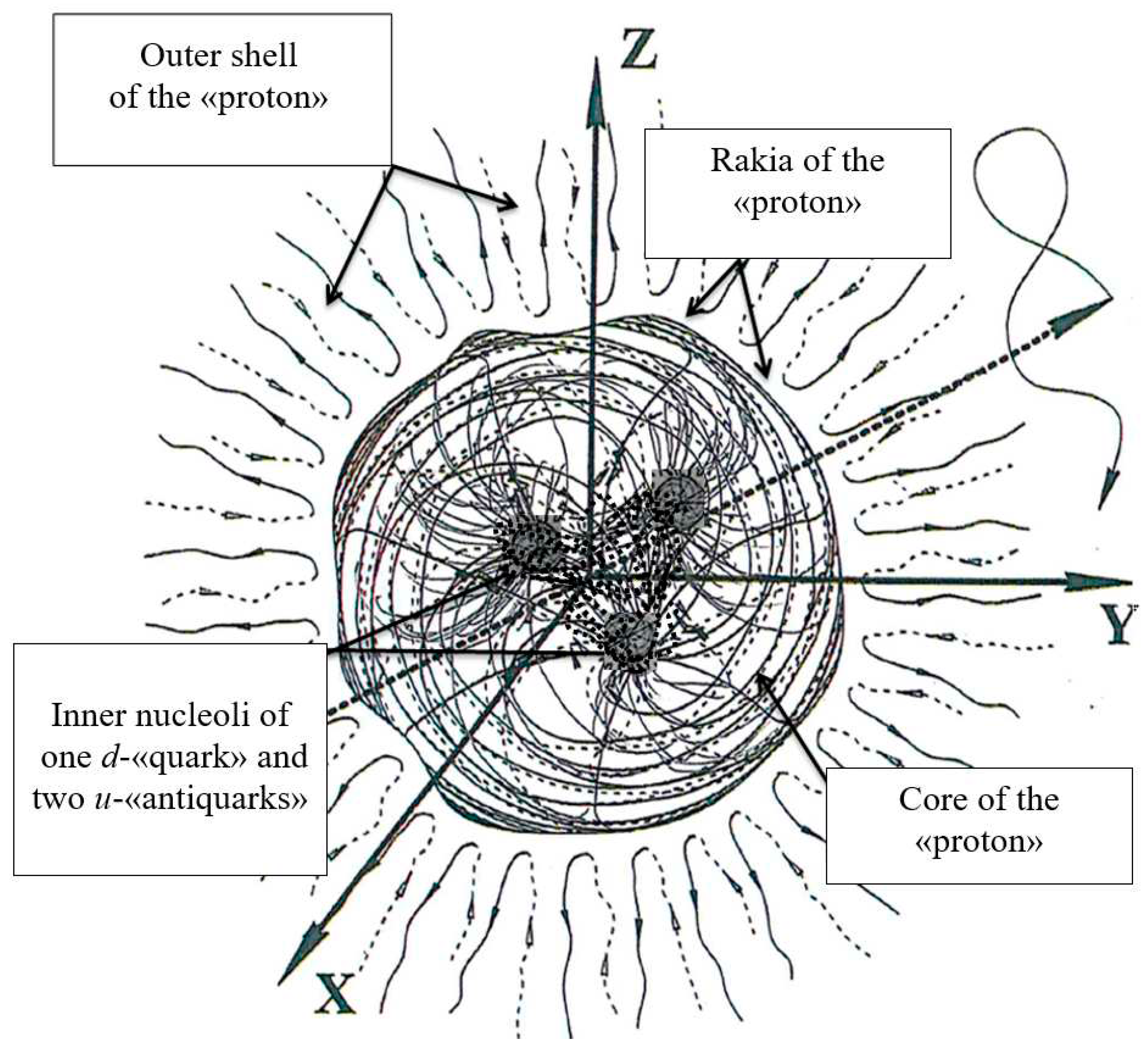
When averaging homogeneous terms in metrics (32.A2) – (40.A2), is obtained a set of metrics (89) – (97) describing the metric-dynamic state of the «positron». However, it should be expected that the radius of the core of the «protons», consisting of the cores of 1 «quark» and 2 «antiquarks», will be greater than the radius of the core of the «positron», because the inner nucleoli of the three «quarks» are difficult to interact, pushing each other away from the common center r = 0 (see Figure 1.A2).
The problem of the confinement of three convex-concave spherical formations: dr+-«quark», ug–-«antiquark» and ub–-«antiquark» is solved by itself, since each xi+-«quark» or xi–-«antiquark» from list (22.A2), except ey– and ey+, are unstable deformed states of vacuum.
Separately dr+-«quark», ug–-«antiquark» and ub–-«antiquark» cannot exist for a long time, because the metrics describing them (32.A2) – (40.A2) are not solutions of Einstein's vacuum equation (8). Only together, they form a stable on average "concave" vacuum formation «proton» (see Figure 1.A2), each averaged layer of which satisfies the stability condition (8).
The centers of the «quarks» dr+, ub– and ub– should wander so chaotically about the common center r = 0 and relative to each other (see Figure 1.A2) so that only on average their centers coincide with the common center of the «proton» cores: <rr> = r = 0, <rg> = r = 0, <rb> = r = 0. Therefore, we are forced to apply not only the metric-dynamic, but also the statistical description of intranuclear processes, which partly considered in [16,17].
The set of metrics (32.A2) – (40.A2) when using the mathematical techniques given in [16,17], allows to extract information about the set of processes and sub-processes occurring both inside the «proton» core and in its "outer shell".
A serious difference between the Algebra of signatures (AS) and the Standard Model of Elementary Particles (SMEP) is that the AS not only largely coincides with the quantum chromodynamics of SMEP, but also extends to spherical objects of any scale.
For example, if in the metrics (1.A2) – (40.A2) we substitute instead of radii:
respectively, the radii from the hierarchical sequence (76):
then we get stellar metric Chromodynamics.
r5 ~ 10–3 cm, r6 ~10–13 cm, r7 ~ 10–24 cm,
r3 ~ 1018 cm, r4 ~ 108 cm, r5 ~ 10–3 cm,
Similarly, if from the same sequence (76) we substitute into metrics (32.A2) – (40.A2), respectively, the radii
then we get galactic metric Chromodynamics, and so on.
r2 ~ 1029 cm, r3 ~ 1018 cm, r4 ~ 108 cm,
3.A2 The «neutron» model in the Algebra of signatures
In modern nuclear physics, it is believed that the neutron consists of two d-quarks with a charge of (–1/3)e and one u-quark with a charge of (2/3)e (where e is the electron charge)
n = ddu.
As a result of this combination, the neutron turns out to be an electrically neutral particle with a zero total charge (–1/3)e + (–1/3)e + (2/3)e = 0.
In Algebra of signatures of a «particle» consisting of three «quarks» («antiquarks») with a zero “electric” environment are not obtained. Since there is not a single additive combination of three of the 16 signatures (37), leading to a zero signature (0 0 0 0), which actually means that all vacuum currents (flows) in the outer shell of such a «particle» are completely mutual compensated [17].
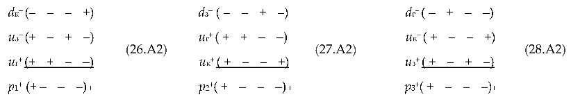
The desired result is achieved in the case of rankings consisting of four signatures. Therefore, an "electrically" neutral «particle» («neutron») can have the following topological (nodal) configurations:
(42.A2)
where (43.A2)
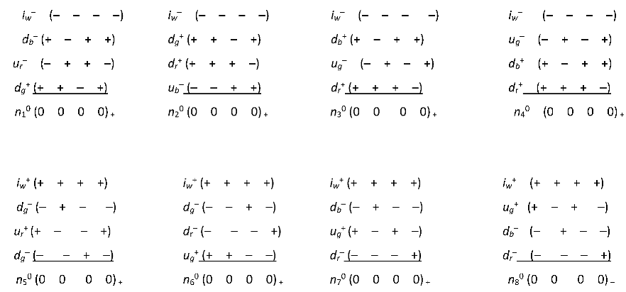 |
iw+ – white iw+-«quark», i.e. 10 metrics of the form (1.A2) with signature (+ + + +);
iw– –white iw+-«antiquark», i.e. 10 metrics of the form (1.A2) with signature (– – – –),
(i from the word invisible). These «quarks» are called white because they are practically invisible inside the core of the «neutron», because in terms of topology, they are "point" and "anti-point" [16,17]. Apparently, therefore, their presence in the core of the neutron was not detected experimentally, and was not taken into account by the Standard Model.
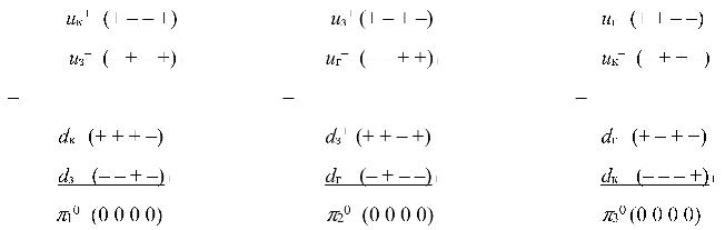
Thus, within the framework of the Algebra of signatures, eight possible states of the «neutron» can be represented as:
which differs from the neutron of the Standard Model (41.A2) by the presence of barely distinguishable iw+-«quark» and iw–-«antiquark».
n10 = iб–dг+dз+uк–, n20 = iб–dк+dз+uг–, n30 = iб–dк+dг+uз–, n40 = iб–dк+dг+uз–,
n50 = iб+dг–dз–uк+, n60 = iб+dз–dк–uг+, n70 = iб+dг–dк–uз+, n80 = iб+dг–dк–uз+,
Due to the complex topological (or signature) metamorphoses inside the core of the «neutron», any permutation of the 4-«quarks-antiquarks» (44.A2) can be rearranged so that inside a given vacuum formation a combination will be obtained, consisting, for example, of a «proton» and an «electron»:
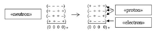
Apparently, this restructuring ("decoupling") a topological node inside the core of a «neutron» and leads to a decay reaction
where νe is an electronic «neutrino».
n → p+ + e– + νe ,
4.A2 The model of the «atom» of hydrogen in the Algebra of signatures
Compared to the neutron, the atom of hydrogen is a much more stable formation.
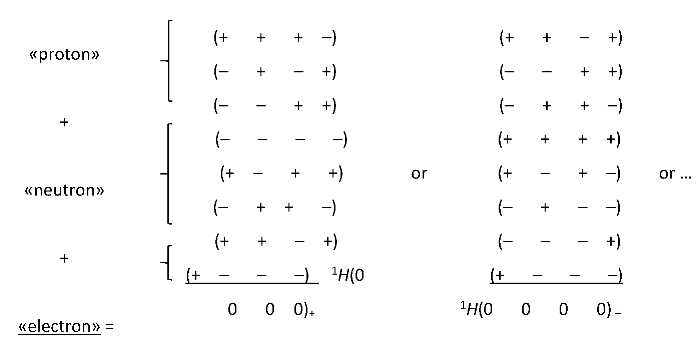
A hydrogen atom (more precisely deuterium) consists of one proton, one neutron and one electron. Within the framework the Algebra of signature, it also turns out that the deuterium «atom» consists of a «proton», a «neutron» and an «electron». The ranking (topological) equivalent of the nodal configuration of such a spherical formation is:
Recall that each signature in these rankings corresponds to 10 metrics of the form (1.A2) with a given signature.
The relationship between the metric extent signature and its topology is shown in §1.11 in [17].
It is possible to make many combinations of signatures similar to (47.A2), which reflects the possibilities of "colored" combinatorics of intranuclear metamorphoses. But the topological configuration of this "knot" always remains the same:
taking into account the topological properties of metrics with corresponding signatures (see §1.11 in [17]), we find that this "knot" consists of 3 intertwined "tori", 4 "oval surfaces" and one "point".
1Н = 3u3die ,
In a similar way, all known chemical elements of the Mendeleev periodic table of elements can be "designed" ("woven"). In this case, the average sizes of the core of «atoms» rA must depend on the number of xi+-«quarks» and xi–-«antiquarks» A that form these "topological nodes"
rA ≈ ½ А1/3r6 ≈ ½ А1/3·10–13 cm.
The Algebra of signatures extends the approach proposed here to the "construction" of multilayer metric-dynamical models of all «atoms» from the periodic table of elements using Fermi’s «quarks» and «antiquarks» (with characteristic sizes of core r4 ~ 108 cm), to "construction" of metric-dynamical models of "stars» and «planets» with the help of Newton’s «quarks» and «antiquarks» (with characteristic sizes of core r4 ~ 108 cm), as well as for the construction of «galaxies» with the help of Galileo’s «quarks» and «antiquarks» (with characteristic sizes of core r3 ~ 1018 cm), as well as on the construction of «metagalaxies» with the help of Einstein’s «quarks» and «antiquarks» (with characteristic sizes of core r3 ~ 1029 cm), etc.
5.A2 Models of «mesons» and «baryons» in the Algebra of signatures
In quantum chromodynamics, mesons are composed of a quark and an antiquark, and are given by the formula
where is the color quark triplet (α = b, ,r); is the color triplet of the antiquark.
Baryons consist of 3 quarks, and are given by the formula
where εαβγ is a completely antisymmetric tensor.
Almost exactly the same way «mesons» and «baryons» are composed within the Algebra of signatures. Consider a specific example: three varieties of π-mesons in the theory of strong interactions (quantum chromodynamics) have the following quark structure:
In the Algebra of signatures, for example, three states of the meson π+ = u– d + is represented as
 where each signature corresponds to a set of 10 metrics of type (1.A2) with a given signature.
In turn, the quark construction
may have the following signature (topological) analogues: (55.A2)
Similarly, within the framework of the Algebra of signatures, all known mesons and baryons of the Standard Model can be "constructed".
The construction of the Algebra of signatures (AS) differs from the constructions of the Standard Model of elementary particles, only by the presence of additional iw+-«quark» and iw–-«antiquark», as well as by the fact that most of the studied AS of multilayer spherical formations consist of intertwining xi+-«quarks» and xi–-«antiquarks», so there is no problem of baryon asymmetry in AS.
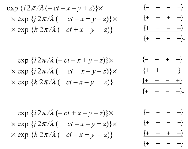
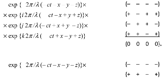
6.A2 Models of «bosons» in the Algebra of signatures
«Bosons» are various types of wave (more precisely, helical harmonic) perturbations in vacuum (see §§1.1 – 1.9 in [17]). In this section, we present the main mathematical models of the Algebra of signatures for these wave disturbances.
- (a)
- "Photon" and "antiphoton"
Spiral harmonic perturbation [17]
we will conventionally call it a «photon» with signature {+ – – –}.
cos{(2π/λ)(сt–x–y–z)} + i sin{(2π/λ)(сt–x–y–z)} = ехр{i (2π/λ)(сt–x–y–z)}= ехр{i(ω t – k⋅ r)}.
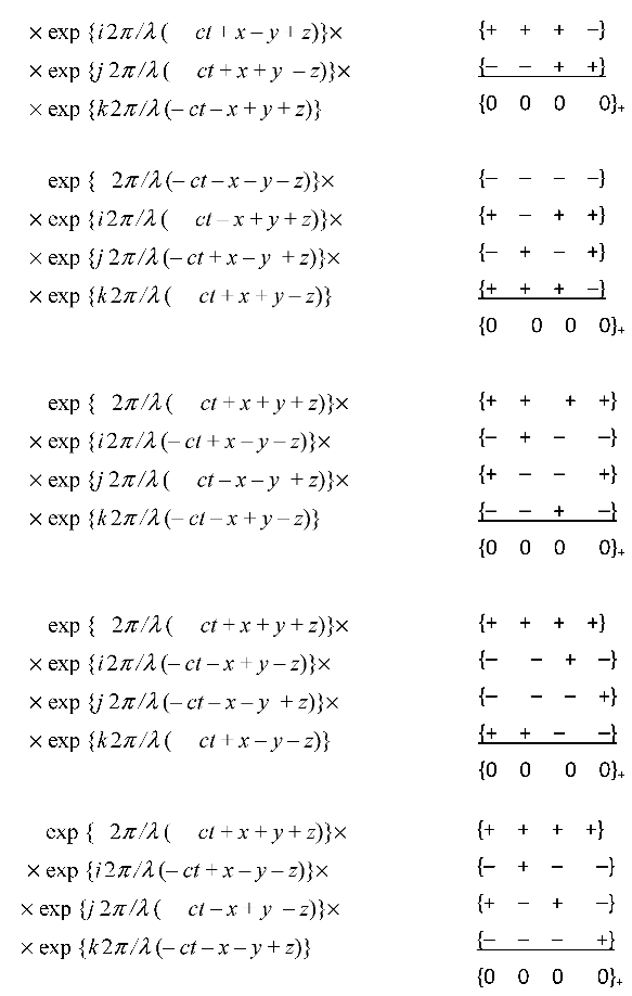
Then a spiral harmonic perturbation propagating in the opposite direction,
we will conventionally call it an «antiphoton» with the stignature {– + + +}.
cos{(2π /λ)(–сt+x+y+z)}+ i sin{(2π/λ)(–сt+x+y+z)} = ехр{i (2π/λ)(–сt+x+y+z)}= ехр –{i(ω t – k⋅ r)}.
The notion of the stignature of an affine space was introduced in §1.8 in [17].
- (b)
- W±-«bosons»
The three color states of the W+-«boson» are given by the following expressions and their corresponding rankings [17] (58.A2)
 |
The three color states of the W–-«boson»: (59.A2)
where i, j, k are imaginary units, form the anticommutative algebra
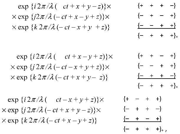 |
i2= j2= k2 = ijk = –1 и ij + ji = 0.
- (c)
- Z0-«bosons»
The six color states of the Z0-«boson» are given by the following expressions and the corresponding rankings [17] (61.A2)
 |
 |
- (d)
- «Graviton» (or «landscapeton»)
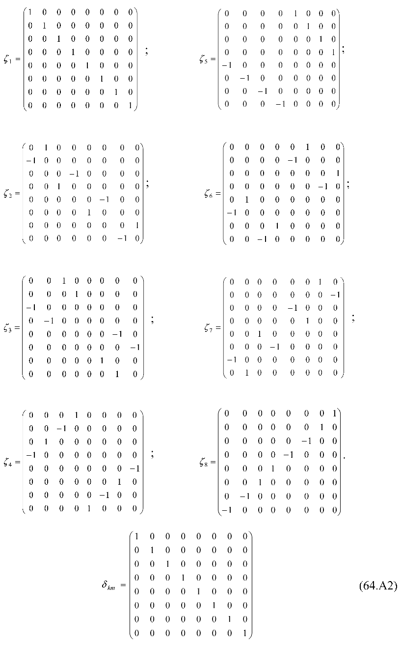
In the Algebra of signatures, there is another «boson», which is called «graviton» (or «landscapeton») [17] (62.A2)
where the objects ζm satisfy the anticommutative relations of the Clifford algebra
where δkm is the Kronecker symbol (δkm= 0 for m ≠ k and δkm= 1 for m = k ). One of the possibilities for determining the objects ζm and the Kronecker symbol δkm is presented below:
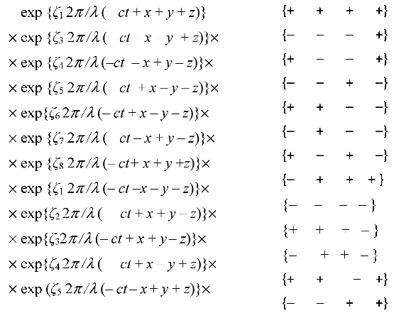 |
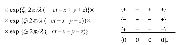 |
ζm ζk + ζk ζm = 0 or m ≠ k , ζm ζm = 1, or ζm ζk + ζk ζm = 2δkm,
 |
7.A2 Conclusions on Annex 2
Metric-dynamic models of all kinds of «neutrinos», «muons» and «antimuons», τ-«leptons», c+,s+,b+,t+-«quarks» and c–,s–,b–,t–-«antiquarks», as well as a geometrized description of the main force interactions: electrostatic, electromagnetic, weak and nuclear are given in chapters 3 – 10 [17].
Thus, taking into account the superposition of stably curved metric spaces with all 16 possible signatures (37)
In the massless Algebra of signatures (or stochastic metaphysics) proposed here, there is no concept of "mass", so there is no need to introduce the concept of a field that provides a mechanism for spontaneous breaking of electroweak symmetry, and, accordingly, about the quanta of this field - Higgs bosons. However, it is possible that in a fully geometrized theory, metric-dynamic models of vacuum formations with characteristics similar to those of these bosons will arise.
Note that if in the aggregate of metrics of the form (78), (88), (12.A2) and (31.A2) instead of:
r5 ~ 10–3 cm is the characteristic radius of the «biological cell»;
r6 ~10–13 cm is the characteristic radius of the «electron» core;
r7 ~ 10–24 cm is the characteristic radius of the «proto-quark» core,
substitute accordingly, for example,
r3 ~ 1018 cm is the radius commensurate with the radius of the «galaxy» core;
r4 ~ 108 cm is the radius commensurate with the radius of the core of a «star» («planet»);
r5 ~ 10–3 cm is the radius commensurate with the size of a «biological cell»;
then we get a practically similar multilayer metric-dynamic description of spherical formations on a stellar-planetary scale.
Whereas, if we substitute
r2 ~ 1029 cm is the characteristic radius of the core of the «metagalaxy»;
r3 ~ 1018 cm is the characteristic radius of the core of the «galaxy»;
r4 ~ 108 cm – characteristic radius, the core of a "star" or «planet»,
then we get a description of spherical formations of a galactic scale, etc.
Thus, in the opinion of the author, has been obtained a universal metric-dynamic model of a closed and, at the same time, Ricci-flat universe, inhabited by countless spherical formations of various scales,
The probabilistic formalism of the Standard Model also remains valid, since the cores and nucleoli of stable vacuum formations constantly move chaotically under the influence of neighboring stable spherical formations and many other vacuum fluctuations. The study of the chaotic motion of the core of a vacuum formation led to the derivation of the Schrödinger equation (see Chapters 3 and 4 in [17]).
References
- Einstein, A. (1916) The Foundation of the General Theory of Relativity // Annalen der Physik. 354 (7): 769. Bibcode:1916AnP...354..769E.
- Einstein, A. (1917) Kosmologische Betrachtungen zur allgemeinen Relativitätstheorie // Sitzungsberichte der Königlich Preußischen Akademie der Wissenschaften. Berlin, DE. part 1: pp.142-152. https://web.archive.org/web/20200329142916/http://echo.mpiwg-berlin.mpg.de/ECHOdocuView?url=/permanent/echo/einstein/sitzungsberichte/S250UZ0K/index.meta.
- Kottler, F. (1918) Uber die physikalischen Grundlagen der Einsteinschen Gravitationstheorie// Annalen der Physik, Vol. 56, pp. 401-462. [CrossRef]
- Glass, E.N., Krisch, J.P. (2004) Kottler-Lambda-Kerr Spacetime, arXiv:gr-qc/0405143v1 , . [CrossRef]
- Desai, S. (2022), Galaxy cluster hydrostatic bias in Kottler spacetime// Physics of the Dark Universe, Vol. 35, 100928, arXiv:2111.14105.
- Bambi, С. (2007) Dark Energy and the mass of galaxy clusters. Phys. Rev. D 75, 083003 arXiv:astro-ph/0703645.
- Nariai, H. (1951). "On a new cosmological solution of Einstein's field equations of gravitation". Sci. Rep. Tohoku Univ. 35: 62.
- Solanki, R. (2021) Kottler Spacetime in Isotropic Static Coordinates // Classical and Quantum Gravity, Vol. 39, № 1, arXiv:2103.10002. [CrossRef]
- Gibbons, G.W. , Warnickand, C.M., Werner, M.C. (2008) “Light-bending in Schwarzschild-de-Sitter: Projective Geometry of the Optical Metric// Class. Quant. Grav. 25, 245009.
- Cohn, J.D. Cohn, J.D. (1998) Living with Lambda//Astrophysics and Space Science, Vol. 259, p. 213–234, arXiv:astro-ph/9807128v2.
- Rindler, W., Ishak, M. (2007) The Contribution of the Cosmological Constant to the Relativistic Bending of Light Revisited// Phys. Rev. D 76, 043006, arXiv:0709.2948.
- Sereno, M. (2007) On the influence of the cosmological constant on gravitational lensing in small systems// Phys. Rev. D 77, 043004, arXiv:0711.1802. [CrossRef]
- Ishak, M., Rindler, W., Dossett, J., (2010) More on Lensing by a Cosmological Constant // Mon.Not. R. As- tron. Soc. 403, 2152, 0810.4956. arXiv:0810.4956 ,. [CrossRef]
- Aghanim N. et al. (Planck Collaboration) (2020). Planck 2018 results. VI. Cosmological parameters (англ.) // Astronomy and Astrophysics. 2020. Vol. 641. P. A6. arXiv:1807.06209. [CrossRef]
- Bachelot, A. (2008) The Dirac system on the Anti-de Sitter Universe//Communications in Mathematical Physics vol. 283, pp.127–167, arXiv:0706.1315,. [CrossRef]
- Batanov-Gaukhman, M. (2021) The Geometrized Vacuum Physics Based Onthe Algebra of Signature. Preprints, 2021060658, doi: 10.20944/preprints202106.0658.v1 https://www.preprints.org/manuscript/202106.0658/v1. [CrossRef]
- Batanov-Gaukhman, M. (2019) Fully geometrized physics from the standpoint of the Algebra of signature// Lambert, ISBN 978-613-9-45278-1, 2019, С. 415. Аvailable in English: http://metraphysics.ru/.
- Gaukhman, M.Kh. (2007) Algebra of signatures "NAMES" (orange Alsigna)// ed. Rabbi Gavriel Davidov. - M.: LKI, ISBN-5203-027780-x, available on the Internet URL: http://alsigna.ru/, section "Orange Alsigna "NAMES"", [in Russian].
- Einstein, A. (1966)// Collection of scientific papers. – M.: Nauka,. Vol.2, p.789.
- Landau, L.D. , Lifshitz E.M. (1971) The Classical Theory of Fields / Course of theoretical physics, V. 2 Translated from the Russian by Hamermesh M. Uni-versity of Minnesota – Pergamon Press Ltd. Oxford, New York, Toronto, Sydney, Braunschwei, p. 387.
- Sedov, L.I. (1994) Continuum mechanics. T.1. – M.: Nauka, [in Russian].
- Novikov, S.P. , Taimanov I.A. (2014) Modern geometric structures and fields. - M.: MTSNMO, 2014. - P. 584 [in Russian].
Figure 3.
Illustration of the interweaving of several affine subspaces forming a multilayer metric space.
Figure 3.
Illustration of the interweaving of several affine subspaces forming a multilayer metric space.
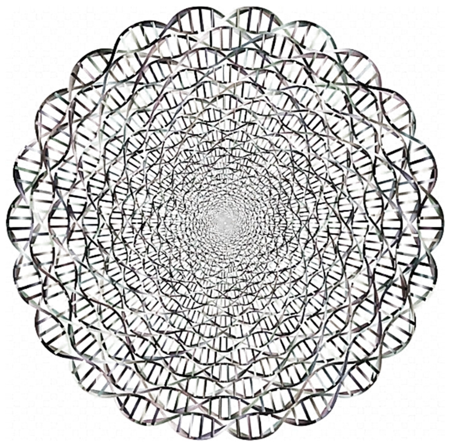
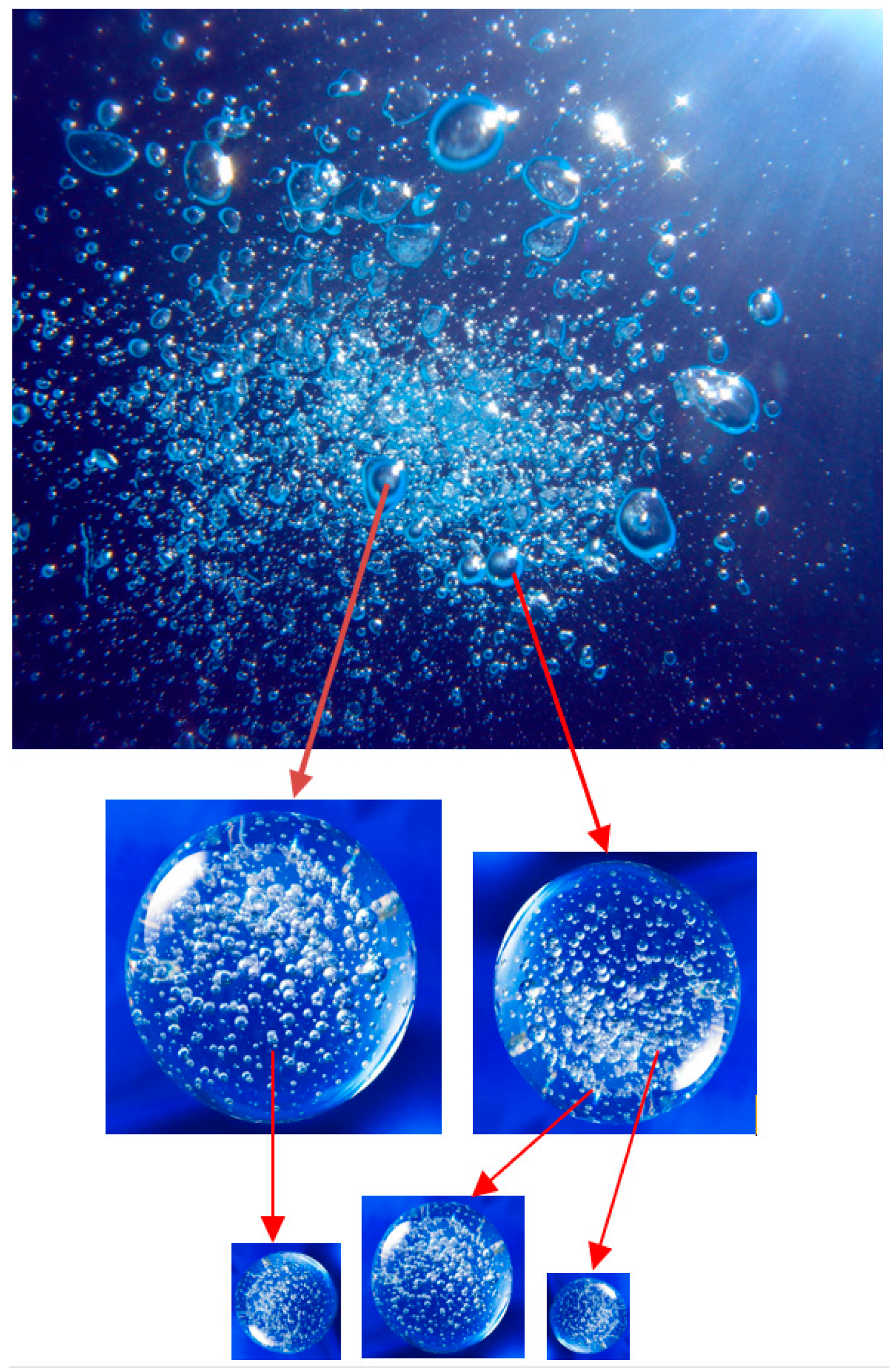
Figure 4.
Illustration of a sequence of “bubbles” within “bubbles” within “bubbles”….
Disclaimer/Publisher’s Note: The statements, opinions and data contained in all publications are solely those of the individual author(s) and contributor(s) and not of MDPI and/or the editor(s). MDPI and/or the editor(s) disclaim responsibility for any injury to people or property resulting from any ideas, methods, instructions or products referred to in the content. |
© 2023 by the authors. Licensee MDPI, Basel, Switzerland. This article is an open access article distributed under the terms and conditions of the Creative Commons Attribution (CC BY) license (http://creativecommons.org/licenses/by/4.0/).
Copyright: This open access article is published under a Creative Commons CC BY 4.0 license, which permit the free download, distribution, and reuse, provided that the author and preprint are cited in any reuse.


