Submitted:
09 January 2023
Posted:
10 January 2023
You are already at the latest version
Abstract
The system identification problem with multiple nonlinearities is relevant. Its decision depends on many factors. These include: feedbacks, the method of connecting nonlinear links, signal properties. They affect the identifiability of the system parameters. We introduced a condition for the excitation constancy for state variables, which considers the S-identifiability of the system. We propose system decomposition by measuring input to identify parameters. Each subsystem has an implicit identification representation. It guarantees obtaining estimates of subsystem parameters based on experimental data. The trajectories boundedness of adaptive system proved in parametric and coordinate spaces. Conditions guaranteeing exponential stability of the system obtained. Systems of self-oscillation generation and nonlinear correction of a nonlinear system consider. Conditions for the trajectories boundedness of the adaptive system obtained for these cases. The influence of nonlinearity and feedback on the system performance estimated.
Keywords:
adaptation
; identification
; identifiability
; stability
; excitation constancy
; Lyapunov vector function
; self-oscillation
1. Introduction
Identification of systems with multiple nonlinearities
studied in several papers. Parametric identification of nonlinearities [1] based on the use of frequency response inversion
based on insufficient data. Sinusoidal tests used to detect nonlinearity. The type
nonlinearity determines based on the analysis of the restoring force function. The
curve fitting method is the basis for estimating nonlinearity parameters. The function
description method [2] used for the parametric
identification of a system with two nonlinear elements. An approach to parameters
estimating of the transfer function of a second-order system suggests in [3]. The system contains dry and quadratic friction.
Harmonic linearization of nonlinearities performed beforehand. Parameter estimates
define as the solution of an equations system.
Identification of nonlinear systems, especially with
multiple local nonlinearities [4] exhibiting disproportionate
ratios of the degree of nonlinearity and present at a single or multiple spatial
location, is a challenging inverse problem. Identification of such complex nonlinear
systems cannot handle by the existing conventional restoring force or by describing
function methods. Meta support vector machine approach [4] uses for the identification of a spring mass system
with several degrees of freedom. Systems identification with multiple nonlinearities
considers in [5]. The approach is based on the
Hilbert–Huang transform. Application stages of this approach and the amplitude-frequency
modulation procedure considered. In [6], a nonlinear
vibration system study with a known structure. Optimization method and recursive
algorithm used to nonlinearity form select from a given class.
The second- and third-order system identification with
dry friction nonlinearities connected in parallel studies in [7]. The identification procedure base on application
of the weighted least squares method. Identifiable conditions obtained and the parameters
finding algorithm for a discrete nonlinear system [8]
with feedback proposed. Nonlinear mechanical vibrations study in [9]. A gray box model or a model based on semi-physical
principles applied. It assumed that observed nonlinearities localized in the physical
space.
The system with two nonlinearities considers in [10]. The structure one nonlinearity is a priori known.
The second nonlinearity approximates by a time series. In [11], the method presented to design mathematical models
for the dynamic system on a set of local nonlinear attachments. Devices installed
in the same primary construction. The identification method uses on the measurements
processing, and the synthesis of the model based on physical laws. The closed system
identification considered in [12]. Frequency methods
applied for estimation system. Convolution schemes use and the learning theory apply
in [13]. Voltaire and Taylor series use to design
models. State space models and learning algorithms based on variational auto-coders
used for nonlinear systems (NS) parameters identification [14].
The review [15] contains
the methods analysis applied for the nonlinear process’s identification in the structure’s
dynamics. Disadvantages of approaches based on linearization, harmonic balance,
and the surface restoring force method note. Identification algorithms based on
the Hilbert frequency transformation proposed in [16].
The chaos theory used to identify bifurcation processes in [17]. The systems Identification with feedback considered
in [18,19]. The proposed approach is based on the
transfer function analysis of the system. The approaches analysis of feedback systems
(FS) identification consider in [20]. The algorithm
determining (AD) parameter estimates asymptotic bias in a nonlinear FS proposed
in [21]. AD based on the correlation analysis between
the system input and the noise. Very often, the FS identification replaces by the
open system parameters assessment [22,23]. A complex
structure is the identification problem of nonlinear FS. A recursive identification
procedure proposes in [24]. The forward channel
describes by an autoregressive model, and the reverse channel describes by a nonlinear
model.
So, the review shows that most of the studies based
on NS frequency identification methods. Estimating approaches to the nonlinearity
structure proposing sometimes. Different procedures apply to linearization of the
nonlinearity from a specified class. Approaches to NS linearization with feedback
considered. The identification problem of systems with multiple nonlinearities is
less studied. The complexity of such systems is the main difficulty for the identification.
Identification approaches and methods of such systems base on localization of nonlinearity.
We propose an approach to adaptive identification of
a system with multiple nonlinearities. This is a complex problem, and its solution
boils down to: (i) the requirements formation on state variables for system parameters
evaluation; (ii) conditions analysis guaranteeing the consideration system nonlinear
properties (S-synchronizability); (iii) synthesis of an adaptive system. We give
a solution to these problems.
2. Problem statement
Consider the system
where is the state vector, is the state matrix, , is nonlinear vector-function, is input (control) vector, , is output vector, , is perturbation vector (measurement errors), is operator to obtain the vector . can be a differential operator.
Information set for
 where .
Assumption 1. Elements , are smooth, one-valued functions and belong to the
class
where is input of a nonlinear element.
The condition may be met in some cases. We apply the model
for the parameters
estimation of matrices , where , , are matrices with tuning parameters.
Problem: construct the model (5) for the system (1)
based on the analysis and assumption 1, and find the tuning laws , и to
whereis the Euclidean norm.
We use the S-synchronizability concept of the system
(1).
3. S-synchronizability of system
S-synchronizability (SS) guarantees the structural identifiability
for the system . SS bases on the property’s analysis of geometric frameworks
[26]. reflects system nonlinear properties, and properties depend on the parameters . An unsuccessful choice of input can give to a so-called
“insignificant” framework [25]. Therefore, the
input (control) choice is the important problem in the identification systems design.
Let the framework closed, and its area is not zero. Denote the height as , where height is the distance between two points on
framework opposite sides. Then the framework , and consequently, the system is identifiable or -identifiable [25]
if:
(i) the input bounded, piecewise, continuous and constantly excited
(see below);
(ii) exists such that .
Structural identifiability conditions of the system.
Let is the domain , is diameter ; , where is acceptable inputs set for the system. The set contains representative inputs.
Definition 1. The input is S-synchronizing the system if the domain of the framework has a maximum diameter on the set .
Remark 1. We understand the system (1), (2) synchronization
as the choice of such the input , which reflects all the features of the framework .
Consider a reference framework . is the structure that reflects all the properties of the nonlinear function
. Let be the diameter of the framework
. exists for a system (1), (2) with an S-synchronizing
input. If , then
where , is a sign of closeness. Subset elements have the property

Consider the framework
. Denote the framework center on the set as , and the area center denote as . Let . Determine secants for fragments , where ; , , , and are parameters .
Theorem 1 [25].
Let the set of synchronizing inputs for the system obtain and (i) exists such that ; (ii) the condition is hold, where are secant coefficients for fragments , . Then the system is -identifiable or structurally identifiable, and .
4. On excitation constancy condition
The condition excitation constant (EC) is important
in parametric identification problems. If the system is nonlinear, then the EC condition
may not be sufficient. The system must be S-synchronized as we consider the nonlinear
properties of the system. The EC condition has the form.
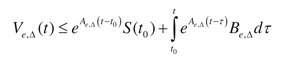
Definition 2. Vector constantly excited with level or has property if
 for and at some interval , where is unity matrix.
The condition (9) has a different form
We use condition (9) next.
Assumption 2. The frequencies set correspond to when have expansion into the Fourier series.
Assumption 3. is the set of allowable input frequencies that ensure
S-synchronizability of the system.
If guarantees the system S-synchronizability by the variable
, then a vector is representative and applicable for the adaptive identification.
Assuming the boundedness, we write the condition EC for as
 where is some number.
5. Structural-parametric approach to system identification
We propose a method for the system identification based on the structural-parametric approach
(SPA) [27]. The SPA realization depends on a priori
information. The system has a complex form. Therefore, the adaptive algorithms
synthesis is based on a priori information about the system structure.
Let the composition of subsystems included in be known. Knowing the output vector dimension the matrix
can decompose into blocks (subsystem ). Perform the subsystems analysis and select subsystems
that contain nonlinearities . Apply SPA to each element . If the subsystem does not contain nonlinearities, then apply
the adaptive identification procedure.
Remark 2. The SPA based on the system S-synchronizability
and the condition (9) fulfillment.
The SPA contains two procedures under uncertainty: (i)
SF1 structural analysis, (ii) parametric (adaptive) identification. These stages
describe in [27].
Remark 3. The system's structural identifiability
(S-synchronizability) affects the connection of subsystems and the correlation of
variables. The relationships analysis excludes influencing relationships and gives
a solution to the system (nonlinearity) structural identifiability problem. The
mutual influence diagram construction is possible only if the condition is true.
Remark 4. The system S-synchronizability evaluation
is based on the framework construction and analysis. [25,26] reflects the
nonlinearity structure of the corresponding subsystem .
Remark 5. Obtained estimates of nonlinearities
structure in are the basis for the adaptive parametric identification
implementation.
Remark 6. We have information about nonlinearity.
Therefore, the structural analysis stage for was not performed.
Remark 7. Structural identification and structural
identifiability based on a single approach. Structural identifiability guarantees
the solution of the structural identification problem for nonlinear systems.
6. Adaptive identification of system
Consider the subsystem , , is a linear operator in (2). Let the information set
be known for . -th order differential equation
corresponds to the
equations system describing the subsystem
 where is state vector, is the first element ; , and are matrices of corresponding dimensions; ; ; is degree polynomial. 2 is a Hurwitz matrix.
Divide the left and right parts of (12) into a degree
polynomial
 where does not coincide with roots of the polynomial . Then (12)
 where , and depend on subsystem parameters and , variables satisfy the
equation
where , and depend on subsystem parameters and , variables satisfy the
equation

Remark 8. The
specificity and structure of the right part (15) define by the matrix and the polynomial .
The representation (15) allows us to estimate the parameters
of on a given set of . Apply the adaptive model
 where
;
, , are tuned parameters. The equation for identification
error
where , , , .
where
;
, , are tuned parameters. The equation for identification
error
where , , , .
Lyapunov function (LF) for the identification algorithms
synthesis has the form . Then
If , have the property , then obtain from
where , , are positive numbers ensuring algorithms convergence.
Get algorithms to adjust model (17) parameters from (20)-(22)
So, the adaptive system
for identification of subsystem parameters describe by the equations (18), (20) – (22).
Denote it as .
Consider LF
where is spur of matrix, , , and .
Let and
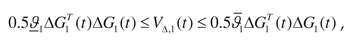
Theorem 2. Let
(i) functions , are positive definite and satisfy conditions
 (ii) is Hurwitz matrix; (iii) variables , have the property . The all trajectories of the system bounded belong to the domain , and the estimate
is valid.
(ii) is Hurwitz matrix; (iii) variables , have the property . The all trajectories of the system bounded belong to the domain , and the estimate
is valid.
The Theorem 2 proof gives in Appendix A.
Let
where , is the sign of the matrices direct sum, , are minimum and maximum matrix eigenvalues, .
The exponential stability proof is based on ensuring
the -property for functions , [29].
Definition 3[29].
A non-positive quadratic form has the -property or if fair
for any , in some bounded domain
where is the Euclidean norm of the vector Y, , .
-property is the constructive completeness sign the
quadratic form . It reduces the properties analysis to the characteristic’s evaluation
of the M-matrix [30].
Lemma 1.has the -property
if matrix and , where are positive numbers, .
The Lemma 1 proof gives in Appendix B.
Lemma 2. If Lemma 1 conditions satisfy, then
has the -property
where .
The Lemma 1 proof gives in Appendix C.
Consider the Lyapunov vector function . Let functions exist such that
Analysis of adaptive system properties (18), (20) –
(22) based on the study of the inequalities system
Apply (31) and obtain a vector comparison system for
(32)
 where , is M-matrix

The stability conditions for the M-matrix have the form [30]
 where are diagonal minors of the matrix .
These conditions have the form for

So, the following statement is true.
Theorem 3. Let (i) positive-definite Lyapunov
functions
 have the infinitesimal higher limit for , ; (ii) matrix and are piecewise continuous bounded and , ; (iii) the equality

Theorem 3 shows if the information matrix is constantly excited, then the adaptive system (18),
(20) – (22) guarantees consistent parameters estimates for system . This statement is valid if (34) is fulfilled.
Remark 9. The EC condition (
) is the base for
the stability proof of the adaptive system. EC indirectly consider when applying
the Lyapunov function. The approach proposed above ensures the
-property for the
Lyapunov function. It bases on consideration the condition
. The Lyapunov function
analysis considers features of adaptive algorithms when the
condition applies.
7. Nonlinear correction of nonlinear system
The system contains
an amplifier with an electric motor and a relay control described by a function. The correcting
device is a nonlinear velocity feedback with a parabolic characteristic

 where is control, is input, .
Equation (13) and polynomials in (13), (14) have the
form

 where , are positive numbers that do not coincide with the
roots of the equation .
where , are positive numbers that do not coincide with the
roots of the equation .
Adaptive model and algorithms for estimating system
parameters (42), (43)

 where , . Equation for error
 where , , .
Denote . The vector tuning law follows from (35)
 where , .
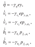
The system (44), and (46) trajectories boundedness follows
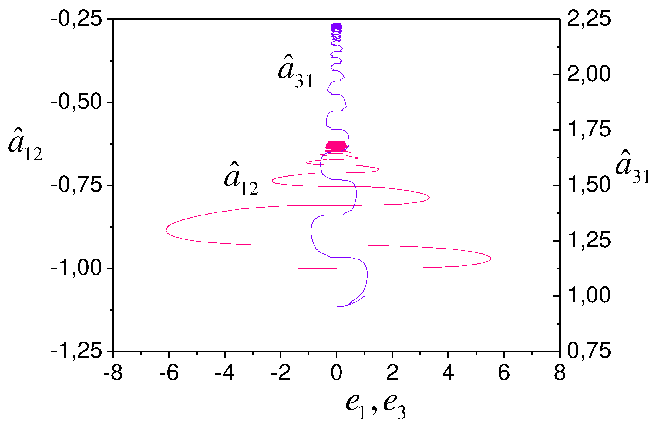
from Theorem 2. The simulation results show in Figures
1-4. Present the model (44) parameter tuning in Figures 1 and 2. Figure 3 reflects the change in the estimation error.
The output form determines the error change. Figure
3 shows also the change in depending on the dynamics of the system output (36).
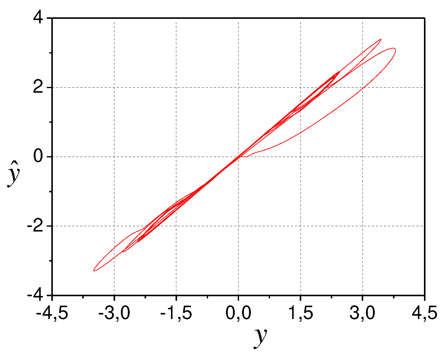
The model adequacy in the output space demonstrates in Figure 4.
Figure 1.
Model (44) parameters tuning.
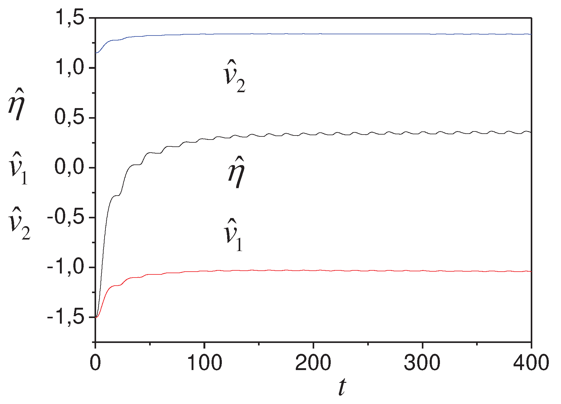
Figure 2.
Model (44) parameters tuning.
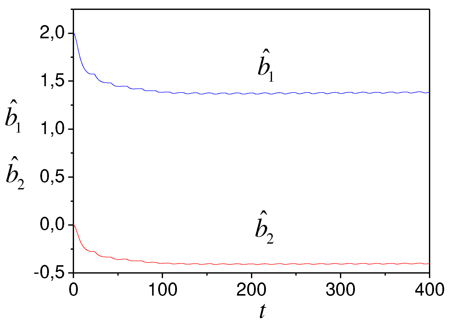
Figure 3.
Changing the estimation error.
Figure 4.
Model adequacy in output space.
Note [32] that the
system (36), (37) is unidentifiable by the function F2 on the measurements set.
In this case, we can use indirect information about the dependence of on . It is true since the relationship between and .
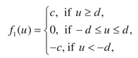
Consider the case when the structure of nonlinearity
is a priori unknown. Use the relationship diagram (RD) [28] for system (36). The relationship between and is significant. Therefore, consider the framework described by the function (Figure 5). belongs to the relay functions class with a dead zone.
Replacing with changes the boundaries of the dead zone. This problem
solves in the identification process. Construct the framework described by the mapping (the structure coincides with ), and the secant
 where . Coefficient of determination is . It indicates the presence of nonlinear properties.
Figure 5.
Framework
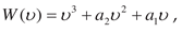
Determine the discrepancy . It contains information about the function . Construction and approximate the curve on the interval . Obtain a model with a quadratic structure. The model
structure coincides with . So, we have performed a structural identification
of the system (36).
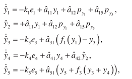
8. Self-oscillation generation system
The self-oscillation system contains (i) a control object
(variables ), (ii) nonlinear (variable ) and linear (variable ) converters, (iii) an amplifier-converter with a nonlinear
actuator (variable )
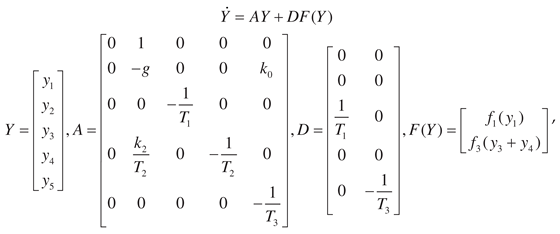 where is time constant, , is input. () is a saturation function with a dead zone

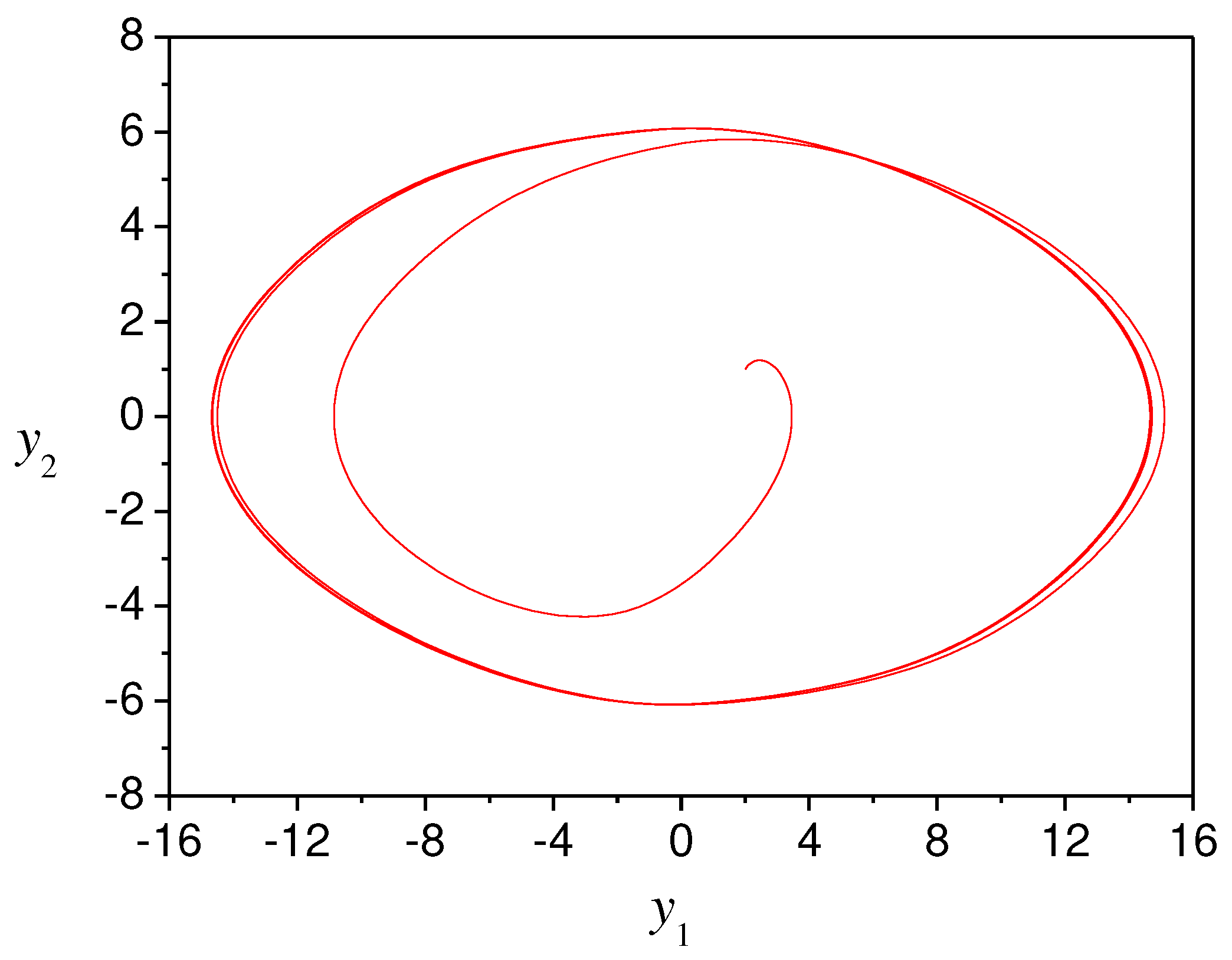
The object phase portrait shows in Figure 6. It shows self-oscillations in the system.
We transform the first two equations of the system (48) using the approach from
Section 6. Present these equations as (38)
and divide (38) by . Transform variables
Figure 6.
Object phase portrait.


The adaptive system for evaluating system (51) parameters
has the form
 where , .
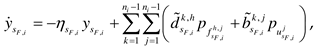
Consider the Lyapunov functions and get adaptive algorithms for tuning system parameters
(52)
 where .
Apply Theorem 2 and get the boundedness of trajectories
in an adaptive system

 where .
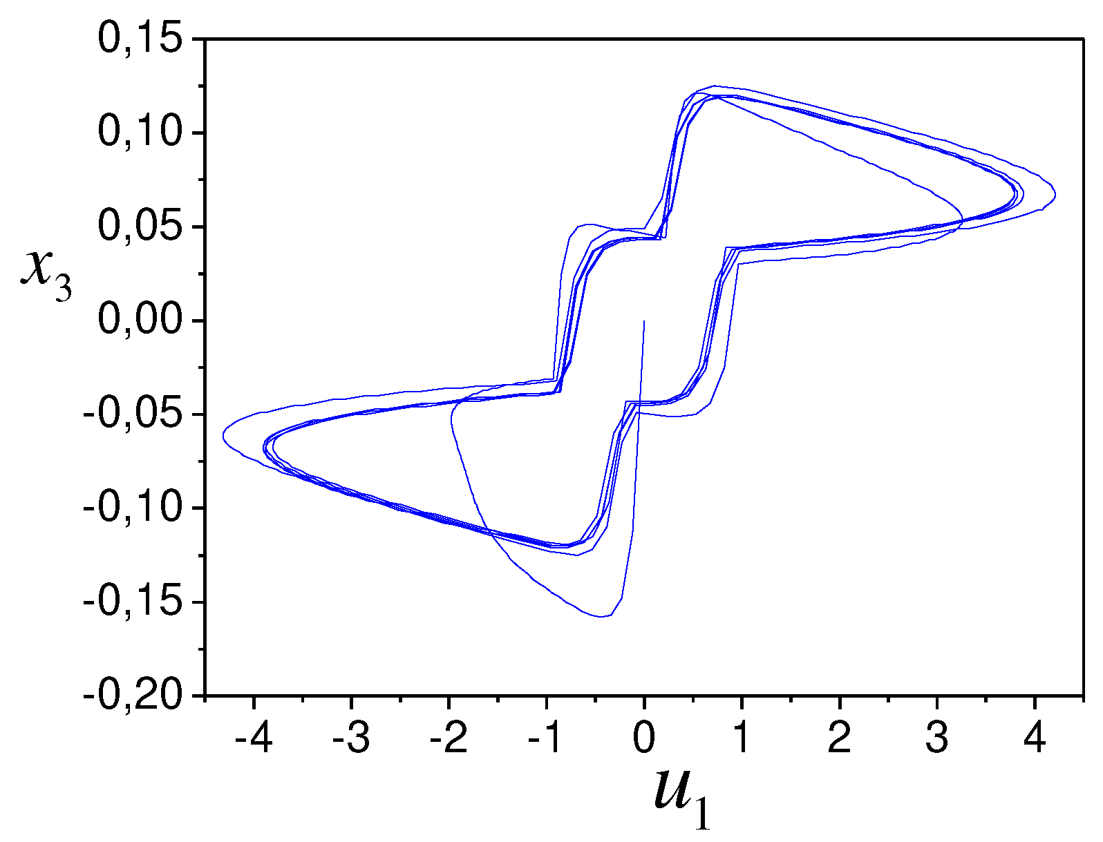
Show the simulation results in Figures 7-10. Figures
7 and 8 represent the system (52) parameters tuning, and Figure 9 shows the change . Results confirm the adaptive system trajectories boundedness.
Figure 7.
Tuning model parameters for estimation
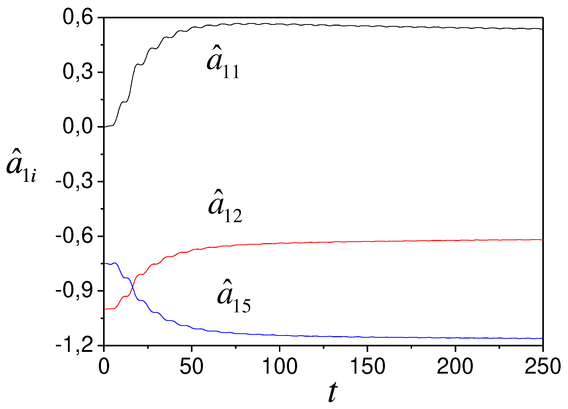
Figure 8.
Tuning model parameters for estimation
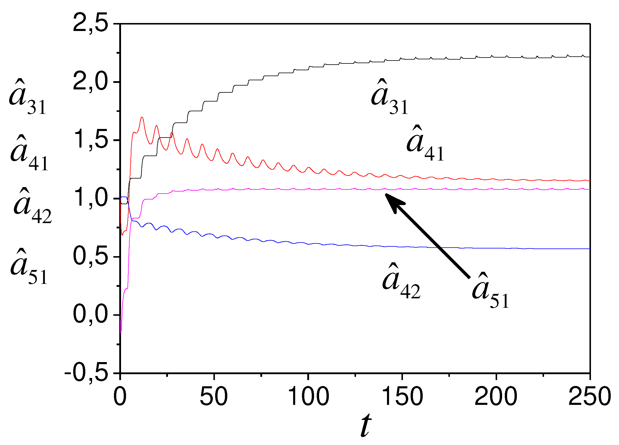
Figure 9.
System errors (52) for various variables (green is , red is , orange is , blue is ).
Tuning parameters in the space shows in Figure 10.
We see that and S-synchronizability execution does not guarantee
the asymptotic stability of the system. Nonlinearity is the reason for such properties
of an adaptive system.
Figure 10.
Tuning parameters in space
Consider Lyapunov functions ,

Theorem 4. Let (i)
positive-definite Lyapunov functions
 have an infinitesimal upper limit at , ; (ii) ,
 where
, , , and are minimum and maximum eigenvalues of the matrix ; (iv) , where , ; (v) ; (vi) the equality fulfilled in the domain , where , , are zero vectors, is number of adjustable parameters, is some neighborhood of a point , ; (vii) the matrix system of inequalities
where
, , , and are minimum and maximum eigenvalues of the matrix ; (iv) , where , ; (v) ; (vi) the equality fulfilled in the domain , where , , are zero vectors, is number of adjustable parameters, is some neighborhood of a point , ; (vii) the matrix system of inequalities
 is valid for , where block-diagonal matrix

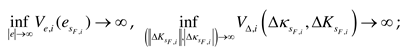
 (viii) the upper solution for satisfies the equation if functions exist such that , , where , is vector element. Then the adaptive system (54), (55) is exponentially
dissipative with the estimate
(viii) the upper solution for satisfies the equation if functions exist such that , , where , is vector element. Then the adaptive system (54), (55) is exponentially
dissipative with the estimate
 if
if

The Theorem 4 proof gives in Appendix D.
As follows from Theorem 4, system (48), (49) limiting
properties depend on nonlinearity, feedback and constant excitation. In particular,
this is true for block 3. The Theorem
4 statement confirms by Figure 11. It reflects
the change of parametric error norm for channels 3-5

Figure 11.
Parametric residual norm.
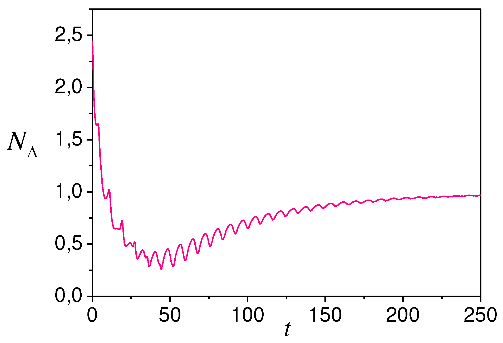
So, the nonlinearities and feedback give biased estimates
for the system parameters (48).
9. Conclusion
We propose the approach to adaptive identification for
systems with multiple nonlinearities. It uses the transformation of equations based
on the experimental data available set. Adaptive identification system designed.
System decomposition into several subsystems is proposed for the adaptation process
simplify. The trajectories boundedness in the adaptive system proved. The S-synchronizability
problem of the system considers, and the excitation constancy condition modification
proposes. The modification considers the requirement for nonlinear system structural
identifiability. The Lyapunov vector function method applies to prove exponential
stability.
Nonlinear correction of a nonlinear system considers.
Adaptive algorithms obtain for estimating system parameters. The system trajectories
limitation proved. A nonlinear system considers for self-oscillation generation
with nonlinear feedback. The adaptive parametric identification system develops.
We study the effect of feedback and nonlinearity. Simulation results confirm theoretical
results.
Appendix A. Proof of Theorem 2
Consider the Lyapunov function (24). has the form of subsystem motions
Apply Theorem 2 condition (i). As , the -subsystem is stable. Integrate
satisfies the Theorem 2 condition (1). Therefore, all
trajectories of the -subsystem belong to the domain
The desired estimate follows from (A.2). ■
Appendix B. Proof of Lemma 1
Consider
Apply the inequality [30]
 and (26). Then
 where is matrix with elements and .
Let and , where are positive numbers. -property for obtains from (B.3)
 where . ■
Appendix C. Proof of Lemma 2
Consider
Let for
 where is system equilibrium position, is some neighborhood of a point , is null matrix, , is some number.
Let , . Apply (C.2) and present (C.1) as
Apply to (С.3) inequalities (B.2), (26) and obtain
 where .
So, -property for
Appendix D. Proof of Theorem 4
Consider the Lyapunov vector function (56). Elements satisfy Theorem 4 condition (i). Ensure the -property for each component . Apply the approach used in proving Lemmas 1 and 2. Consider the proof procedure with the example . has form
Apply to (D.1) inequalities (B.2) and obtain

Let , , , , , are minimum and maximum eigenvalues of the matrix . Theorem 4 condition (iii) holds for . Then (D.2)

So, the -property obtain for . Consider
 where , , . levels the EC property, as the nonlinear properties of the system effect.
Apply Theorem 2 and get the adaptive system trajectories boundedness. Then (D.4)
 where is uncertainty appearing at , .
Apply the above approach and get the - property for the remnants
 where .
Consider components and use the approach used for Lemma 2 proving. Let the condition for , where is system equilibrium position, is some neighborhood of a point , , are corresponding variables in (48). Then
 where , . Apply (B.2) and get the -property for

Similarly, obtain the -property for elements
 where is the result of the violation of the EC condition. The boundedness follows from Theorem 2.
The derivative satisfies the matrix system of inequalities
 where , ,

The comparison system is fair for (D.10)
 if functions exist such that the comparison system is fair for (D.10)
 where , is elements of the vector .
Form shows that system (48) channels are isolated at the level of stability research. Therefore, perform the analysis for each channel. is an M-matrix [30]. The major minors positivity is the condition for the asymptotic stability of the adaptive system. Have

We see that the limiting properties (48) depend on the nonlinear properties of the system, feedback, and constant excitation. In particular, this is true for channel 3 in (D.10). ■
References
- Aykan M., Özgüven H.N. (2012) Parametric Identification of Nonlinearity from Incomplete FRF Data Using Describing Function Inversion. In: Adams, D., Kerschen, G., Carrella, A. (eds) Topics in Nonlinear Dynamics, Volume 3. Conference Proceedings of the Society for Experimental Mechanics Series. Springer, New York. [CrossRef]
- Zhao Z., Li C., Ahlin K., Du. H. (2016) Nonlinear system identification with the use of describing functions – a case study, Vibroengineering PROCEDIA, 8, 33-38.
- Pavlov Y.N., Nedashkovskii V.M., Tihomirova E.A. (2015) Identification of Nonlinear Dynamic Systems Possessing Some Nonlinearities, Science and Education of the Bauman MSTU, 07, 217–234.
- Prawin J., Rao A.R.M. & Sethi A. (2020) Parameter identification of systems with multiple disproportional local nonlinearities, Nonlinear Dyn, 100, 289–314. [CrossRef]
- Pai P. F., Palazotto A. N. (2008) Detection and identification of nonlinearities by amplitude and frequency modulation analysis, Mechanical Systems and Signal Processing, 22(5), 1107-1132.
- Safari S., Monsalve J. M. L. (2021) Direct optimization based model selection and parameter estimation using time-domain data for identifying localised nonlinearities, Journal of Sound and Vibration, 501, , 116056.
- Noël J., Schoukens J. (2018) Grey-box state-space identification of nonlinear mechanical vibrations, International Journal of Control, 91(5).
- Li C. (2021) Closed-loop identification for a class of nonlinearly parameterized discrete-time systems, Automatica, 131, 109747. [CrossRef]
- Noël J.P., and Schoukens J. (2018) Grey-box State-space Identification of Nonlinear Mechanical Vibrations, International Journal of Control, 91(5), 1118-1139.
- Binczak S., Busvelle E., Gauthier J.-P., Jacquir S. (2006) Identification of Unknown Functions in Dynamic Systems. https://pageperso.lis-lab.fr/eric.busvelle/papers/bioid.pdf.
- Singh A. and Moore K. J. (2021) Identification of multiple local nonlinear attachments using a single measurement case, Journal of Sound and Vibration, 513, 116410. [CrossRef]
- Paul Van den Hof. (1997) Closed-loop issues in system identification. In: Y. Sawaragi and S. Sagara (Eds.), System Identification (SYSID'97), Proc. 11th IFAC Symp. System Identification, Kitakyushu, Japan, 8-11 July 1997. IFAC Proceedings Series, 3, 1547-1560.
- Andersson C., Ribeiro A. H., Tiels K., Wahlström N. and Schön T. B. (2019) Deep convolutional networks in system identification, IEEE 58th Conference on Decision and Control (CDC).
- Gedon D., Wahlström N., Schön T. B., Ljung L. (2021) Deep State Space Models for Nonlinear System Identification. arXiv:2003.14162v3 [eess.SY]. [CrossRef]
- Kerschen G., Worden K., Vakakis A. and Golinval J.-C. (2006) Past, present and future of nonlinear system identification in structural dynamics, Mechanical Systems and Signal Processing, Elsevier, 20 (3), 505-592. [CrossRef]
- Holmes P. (1982) The dynamics of repeated impacts with a sinusoidally vibrating table, Journal of Sound and Vibration, 84, 173–189.
- Azeez M.A.F., Vakakis A.F. (1999) Numerical and experimental analysis of a continuously overhung rotor undergoing vibro-impacts, International Journal of Non-Linear Mechanics, 34, 415–435.
- Van den Hof P. (1998) Closed-loop issues in system identification. Annual Reviews in Control, 22(0), 173 – 186.
- Aljamaan, I. (2016) Nonlinear Closed-Loop System Identification in The presence of Non-stationary Noise Source (Unpublished doctoral thesis). University of Calgary, Calgary, AB.
- Forssell U., Ljung L. (1999) Closed-loop identification revisited, Automatica, 35, 1215-1241. [CrossRef]
- Mejari M., Piga D. and Bemporad A. (2018) A bias-correction method for closed-loop identification of Linear Parameter-Varying systems, Automatica, 87, 128–141. [CrossRef]
- Piga, D., Tуth R. (2014) A bias-corrected estimator for nonlinear systems with output-error type model structures, Automatica, 50(9), 2373–2380.
- Gilson, M. and Van den Hof, P. (2001) On the relation between a bias-eliminated leastsquares (BELS) and an IV estimator in closed-loop identification, Automatica, 37(10), 1593–1600. [CrossRef]
- Song G., Xu L. Ding F. (2019) Recursive least squares algorithm and stochastic gradient algorithm for feedback nonlinear equation-error systems. International Journal of Modelling, Identification and Control, 32(3-4), pp. 251-257.
- Karabutov N. (2021) Introduction to the structural identifiability of nonlinear systems; URSS/ Lenand: Moscow.
- Karabutov N.N. (2020) S-synchronization Structural Identifiability and Identification of Nonlinear Dynamic Systems. Mekhatronika, Avtomatizatsiya, Upravlenie, 21(6), 323-336. (In Russ.).
- Karabutov N. (2018) Structural-parametrical design method of adaptive observers for nonlinear systems, International journal of intelligent systems and applications, 10(2), 1-16. [CrossRef]
- Karabutov N. (2018) Geometrical frameworks in identification problem, Intelligent control and automation, 12(2), 17-43. [CrossRef]
- Karabutov N. (2017) Adaptive observers with uncertainty in loop tuning for linear time-varying dynamical systems, International journal intelligent systems and applications, 9(4), 1-13. [CrossRef]
- Gantmacher F.R. (2000) The Theory of Matrices; AMS Chelsea Publishing: Reprinted by American Mathematical Society.
- Karabutov N. (2022) Structural Identifiability of Feedback Systems with Nonlinear Adulterating, Contemporary Mathematics, 3(2), 257-269. [CrossRef]
- Karabutov N. (2021) Structural Identifiability of Systems with Multiple Nonlinearities, Contemporary Mathematics, 2(2) 141-161. [CrossRef]
- Barbashin E.A. (1970) Lyapunov function; Nauka: Moscow.
Disclaimer/Publisher’s Note: The statements, opinions and data contained in all publications are solely those of the individual author(s) and contributor(s) and not of MDPI and/or the editor(s). MDPI and/or the editor(s) disclaim responsibility for any injury to people or property resulting from any ideas, methods, instructions or products referred to in the content. |
© 2023 by the authors. Licensee MDPI, Basel, Switzerland. This article is an open access article distributed under the terms and conditions of the Creative Commons Attribution (CC BY) license (http://creativecommons.org/licenses/by/4.0/).
Copyright: This open access article is published under a Creative Commons CC BY 4.0 license, which permit the free download, distribution, and reuse, provided that the author and preprint are cited in any reuse.


