Submitted:
23 December 2022
Posted:
05 January 2023
You are already at the latest version
Abstract
This manuscript compares deterministic artificial intelligence to model following control applied to DC motor control, including evaluation of the threshold computation rate to let unmanned underwater vehicles correctly follow the challenging discontinuous square wave command signal. The approaches presented in the main text are validated in MATLAB®, where the motor process is discretized at multiple step sizes, which is inversely proportional to the computation rate. The performance is evaluated by the error mean and standard deviation. With a large step size, discrete deterministic artificial intelligence shows a larger error mean than the model-following self-turning regulator approach (benchmark selection). However, the performance gets optimized with the step size decreased. The error mean is close to the continuous deterministic artificial intelligence when the step size is reduced to 0.2 seconds, which means that the computation rate and the sampling period restrict discrete deterministic artificial intelligence. In that case, the continuous deterministic artificial intelligence is the most feasible and reliable selection for future applications on unmanned underwater vehicles since it is superior to all the approaches with multiple computation rates.
Keywords:
artificial general intelligence
; intelligent robotics
; oceanic robots
; unmanned underwater vehicle (UUV)
; deterministic artificial intelligence
; model-following
; recursive least squares
; marine actuators
; self-tuning regulators
1. Introduction
Over the past decades, the increasing threats and the emerging situation posed a significant challenge to the coast guard worldwide. The Department of the Navy is moving to innovate and adapt new technology to build a more lethal and distributed naval force for the future [1]. The US Department of Defense seeks to tackle the threat problem using unmanned technologies and applications. Unmanned underwater vehicles seem to be one of the reliable solutions for successful maritime interdiction missions [2] emphasizing the automation of DC motor control.
The vehicle is controlled by the fin-shape actuator shown in Figure 1a,b. The unmanned underwater vehicle can sail along the disparate trajectory by sending a command signal to the motors connected to the actuator (e.g., Figure 1). In this manuscript, the efficacy of the motor control techniques is evaluated with respect to system discretization.
Sarton formulation autopilot techniques using differential thrust for Aries autonomous underwater vehicle in 2003 [6], while Tan focused application to horizontal steering control during docking [7]. Sarton sought advantages in differential thrust to counter wind and wave disturbances while surfaced by creating different motor voltages supplied to each propeller motor. Seeking autonomous recovery or docking operations, Tan focused on the capability of vehicle track and steer itself accurately despite constant perturbation by wave motion effects necessitating accurate acoustic homing during the final stages of the docking with high update rates of acoustic systems. The Aries vehicle was experimentally tested to have an update rate of only about 0.3 Hz. These delayed data can potentially cause a false commanded reference input to the tracking system in between the updates and cause Aries to miss the moving cage’s entrance motivating high interest investigating systems that prove efficacy at such low data rates. More recently, Wang et al. [8] proposed fault-tolerant control based on nonlinear programming furthermore motivating investigation of efficacy at low data rates since such methods ubiquitously require increased computational times.
Least squares parameter identification was proposed by Dinç to estimate hydrodynamic coefficients for autonomous underwater vehicles in the presence of measurement biases [9], while this present manuscript illustrates application of such techniques to estimation of actuator motor parameters. Gutnik, et al. illustrated how the efficacy of such approaches manifest in operational capabilities for autonomous, near-seabed visual imaging missions [10], particularly as it pertains to thrust allocation for path following.
The development of adaptive and learning systems has a long history that is presently culminating in a very recent, distinguished lineage in the literature [4,11,12,13,14], already bestowing three major publication awards, validating the contemporary interest in continued developments. Many techniques are available from this long lineage as alternatives benchmarks for comparing newly proposed methods. Rathmore focused on artificial intelligence applying robust steering control based on tuning of PID controller using the so-called genetic algorithm and the harmonic search algorithm [11]. In 2020, so-called deterministic artificial intelligence was proposed for controlling autonomous unmanned underwater vehicles [12]. The method is based on the self-awareness assertion in the feedforward process dynamics. The feedback signal was formatted by Koo as an adaptive & learning system (proportional derivative feedback and 2-norm optimal least squares). [13] As a duplication and continuation of Koo's work in [13], this manuscript provides an in-depth comparison between the performance of the deterministic artificial intelligence and declared benchmark approaches with iterated step sizes. The performance evaluation mainly focuses on the ability to track the command signals represented by challenging square wave trajectories.
Bernat introduced a speed control approach [15] based on a model-reference adaptive control algorithm for torque load and ripple compensation. Gowri described a direct torque control as one approach focused on discontinuities in rapid modulating commands [16]. Moreover, Rathaiah [17] and Haghi [18] both proposed extremum-seeking adaptive control of first-order systems, which is similar to the approach applied to the vehicle automation control described in [19]. The methods are similarly tested and compared with discontinuous step and square wave inputs. For DC motors, tracking discontinuous step functions and square wave function is challenging since overshoot occurs at the square wave's discontinuities, significantly influencing the tracking performance of nonlinear adaptive control approaches. The difficulty is validated by Vidlak’s very contemporary example in Figures 24 and 26 in [20]. This facet is also elaborated by Vidlak’s work on tracking performance of self-turning regulators [20] and model reference adaptive control [21].
A similar phenomenon is revealed in Section 3 of this manuscript for the error distribution comparison of different algorithms. This manuscript describes a duplication and continuation of the work presented in [13], which is also work based on its prequel research by Shah [14], where model-following self-turning regulators [22] are chosen as the comparative benchmark approach.
The learning approach evaluated in this manuscript stems from Slotine [23] and the nonlinear adaptive method for robotics [24]. The technique was quickly transformed to expression in coordinates of the body reference frame [25]. In [26], the tunability of feedback and feedforward elements are demonstrated, substantiating the self-awareness statements of deterministic artificial intelligence. [27] As described by Fossen in [28], alternative trajectory tracking control mechanisms based on classical proportional, integral, derivative control; linear-quadratic regulator; feedback linearization; nonlinear backstepping; and sliding mode control are presented. Some approaches are applied to the ocean vehicle mentioned in [29]. The efficacy of such systems is also simulated in [30]. Lorenz and his students also used and evaluated the feedforward element in [31,32,33,34,35,36,37]. The fault-tolerance [33], loss reduction [34], loss minimization [35], dead-beat control [36], and self-sensing [20,37] are evaluated and extended from the vehicle to the actuator control circuit. As described in [19,20], the precursor using the physics-based dynamics for virtual sensing, which follows the illustration of optimality and self-sensing, is applied explicitly to DC motors.
This manuscript continues the investigation of Koo [13] in a deterministic artificial intelligence learning approach following the recommendation provided by Shah [14]. In Section 3, the comparison analysis of computational rate is evaluated for the adaptive and learning methods. More step sizes are applied to the compared approaches to assess their performance based on the error mean and error standard deviations.
- Main Conclusion of the study
As a sequel of Koo [13], multiple propositions are evaluated in Section 2. Validating research is included in Section 3, with direct comparisons between each algorithm based on canonical figures of merit.
- Recommendation of key threshold discretization and computational speed to duplicate the results of the original prequel [3].
- Validation of the first sequel's [14] identification of paramountcy of discretization and computational speed.
- Validation of the second sequel's [13] identification of deterministic artificial intelligence performance and recommended selection of algorithms.
2. Materials and Methods
This section includes sufficient detail for others to replicate the published result. A truth model for motor dynamics and a model-following self-tuner is described in Section 2.1 and Section 2.2, while the newest method (deterministic artificial intelligence) is elaborated in Section 2.3. Deterministic artificial intelligence is a learning method that first asserts self-awareness, and then learns in the context of that self-awareness alone.
2.1. Truth Model for Motor Dynamics
As described by [31], considering a continuous-time process and precisely a normalized model for a DC motor [13], the transfer function is described in equation (1).
equation (2) shows the z-transform for the discrete-time signal under the frequency domain. With the MATLAB® function provided in Appendix A, a time step of 0.5 seconds is used as the initial continuous-time process. (z) and represent the control signal and output under the z-transform domain.
The final form can be written as equation (3)
2.2. Model-Following Self Tuner
As shown in Figure 3.3 in [22], a dynamic feedforward is applied to the input , and negative dynamic feedback is applied on output . In that case, the process input can be produced. The system can be described in equation (4) and equation (5), where (z) and represent the control signal and output under the z-transform domain.
Due to the designed topology, some cancellation is applied on equation (5), where represents the canceled zeros, represents uncancelled represents a scalar multiple to the system, and represents the pole-zero cancellation used to generate the desired system transfer function. [14]
is set to 1 since no process zero cancellation should be included in the demonstrated control design. As described in [22], R, S, and T are first order. By manipulations of equation (6), the coefficient of R, S, T can be defined as equation (7)-(9) in terms of estimated and desired process parameters.
Then, the control signal into the process can be described by equation (10) and equation (11) after adding feedforward and feedback.
As described by [22], will obtain the system to get a unity gain which is essential for attaining zero asymptotic tracking error.
2.3. Deterministic Artificial Intelligence
Deterministic artificial intelligence requires self-awareness assertion, which can be established by isolating in the left-hand side of equation (3). [13] equation (12)–(14) shows the manipulation to express the to the product of matrix of known, , and unknown, . The unknown matrix, , is the learning parameters from PD feedback control that can generate the process input. is the regression form of input .
Apply feedforward control and modify the state form to in equation (3). Then, the desired trajectory can be computed. To learn the updated feedback parameters , The rough initial estimates of the feedback parameters along with the values of output and regression are used in recursive least squares. [13] Convert the transfer function in equation (1) back into the ordinary differential equation reparametrized as in equation (13). The continuous system can be evaluated by using the deterministic artificial intelligence method. Besides, as described in [27], the optimal feedback adjustment can be applied to the system to learn the feedback parameters in the discrete environment, shown in equation (15).
The control input and sinusoidal trajectory (given by equation (16)) could be obtained by putting the updated and optimal feedback parameters back into equation (13). The and in equation (15) are the original and target states, respectively.
3. Results
This section shows the comparison between the model-following self-tuner control and discrete deterministic artificial intelligence in Section 3.1. Compared with the resultant in [13], a larger step size is applied to validate the statement mentioned by Koo: discrete deterministic artificial intelligence is more susceptible to larger step sizes but more efficacious with a smaller step size. [13] Moreover, the comparison between continuous deterministic artificial intelligence and discrete deterministic artificial intelligence is shown in Section 3.2.
3.1. Model-following Self-tuner Control v.s. Deterministic Artificial Intelligence
Comparing the error mean and standard deviation under four different step sizes, the deterministic artificial intelligence approach shows a more tracking error than the model-following approach when using larger sampling periods (faster computation rates). As shown in Table 1., this phenomenon gets exacerbated with even a slight step size increase. It is obvious to observe through Figure 2 below that there is a discrepancy between those two approaches at large step size. The output signal from deterministic artificial intelligence shows a large oscillation at the beginning, while the model-following output signal tracks the command signal immediately.
According to Table 1, when the step size increases from 0.5 to 0.6 seconds, the mean tracking error rises sharply, 242 times the mean error of the model-following approach. The standard deviation also increases dramatically, which is 49 times the standard deviation of the model-following method.
However, the performance gets significantly more reliable when the step sizes get smaller. When the step size is reduced to 0.20 seconds, the mean error of the deterministic artificial intelligence approach decreases to 10% of it with a 0.5-second step size. The standard deviation also reduces to 1/3 of it with a 0.5-second step size. For the output of deterministic artificial intelligence, there is an overshoot at discontinuous and follows the input signal with a small tracking error, which Koo [13] also mentions. In contrast, there is a degradation in the performance of the model-following approach when the step size is reduced from 0.6 to 0.2 seconds. An oscillation can be observed as the step size gets smaller.
3.2. Discrete deterministic artificial intelligence v.s. Continuous deterministic artificial intelligence
Table 2 shows the comparison of error distribution between discrete deterministic artificial intelligence and continuous deterministic artificial intelligence. Overall, as already discussed in the material and method section, deterministic artificial intelligence is less efficacy with a large step size, which can be observed below. When the step size changes from 0.5 to 0.2 seconds, discrete and continuous deterministic artificial intelligence performance increases significantly. According to the error mean in Table 2, the mean error between those two deterministic artificial intelligence is close to each other with a small step size. The difference is just about 7%.
Although the error standard deviation of discrete deterministic artificial intelligence is half that of continuous deterministic artificial intelligence, a minor standard deviation doesn't represent better performance. The larger standard deviation of continuous deterministic artificial intelligence is caused by the more prominent initial oscillation in the initial transient, shown in Figure 3. After the oscillation section, the performance of continuous deterministic artificial intelligence is expected to exceed the discrete deterministic artificial intelligence since it has a marginal tracking error. MATLAB® obtains the results of Section 3. The code is included in Appendix A to help with replication or further construction based on this article.
4. Discussion
Table 3 and Table 4 show the performance improvement of different algorithms. This manuscript validates the deterministic artificial intelligence approach's ability to track the discontinuous command square wave compared with alternative techniques. The exemplary performance of continuous control is examined. Further discretization could be applied to obtain better performance for continuous control. As described in Table 3 of [13], different discretization methods, such as zero-order hold (ZOH), bilinear approximation (Tustin), and linear interpolation (FOH), could significantly reduce the tracking error with large step sizes.
As shown in Figure 2 and Figure 3, this manuscript included the control effects for different control algorithms. Moreover, the performance of different algorithms at disparate step sizes is also compared in previous tables and figures. Besides, as further research of the article written by Koo [13], more step size of different control methods was applied in this manuscript further to validate the deterministic artificial intelligence performance over various situations. Overall, the discrepancy of the output signal from the different algorithms decreased with the step size reduced. Eventually, it became negligible. Discrete deterministic artificial intelligence seems to have the best performance under a slow computation rate (small step sizes), and continuous deterministic artificial intelligence is the next. However, since the continuous deterministic artificial intelligence is superior with various computation rate compared with other approaches overall, it might be the most feasible and reliable selection for future applications on unmanned underwater vehicles.
The future research recommendation will be replicating all the benchmarks for the sequel study and validating more parameters influenced by different control algorithms. Given these promising results, it is important to continue researching and refining deterministic artificial intelligence to improve its performance further. In particular, future research should focus on eliminating the sole transient that occurs on initial startup, as this could lead to even more accurate and stable estimates. Many potential approaches could be used to address this issue, including the development of new computational techniques, the incorporation of additional data or model assumptions, and the use of different types of algorithms or models. By carefully exploring these options, it may be possible to develop deterministic artificial intelligence that is even more effective at estimating parameters in various situations.
Author Contributions
Conceptualization, Z.W. and T.S.; methodology, Z.W. and T.S.; software, Z.W. and T.S.; validation, T.S.; formal analysis, Z.W. and T.S.; investigation, Z.W. and T.S.; resources, T.S; writing - original draft preparation, Z.W.; writing - review and editing, Z.W. and T.S.; supervision, T.S.; funding acquisition, T.S. All authors have read and agreed to the published version of the manuscript.
Funding
This research received no external funding.
Data Availability Statement
Data supporting reported results can be obtained by contacting the corresponding author.
Acknowledgments
The code used to generate data and figures in this manuscript is adapted from the Appendix A of Koo Mo Koo and Henry Travis's article [13].
Conflicts of Interest
The authors declare no conflict of interest.
Appendix A
The appendix contains topologies crucial to understanding and reproducing the research published in this manuscript. The code should be run by MATLAB®.
Appendix A.1. Discrete deterministic artificial intelligence
clear all; clc; close all;
%% DISCRETIZATION
% B=[0 0.1065 0.0902];A=poly([1.1 0.8]);
% Gs = tf(B,A);
% a1=0;a2=0;b0=0.1;b1=0.2; %Shah’s
Bp=[0 0 1];
Ap=[1 1 0];
Gs=tf(Bp,Ap); %Create continuous time transfer function
Ts=0.5;
Hd=c2d(Gs,Ts,'matched'); % Transform continuous system to discrete system
B = Hd.Numerator{1};
A = Hd.Denominator{1};
b0=0.1; b1=0.1; a0=0.1; a1=0.01; a2=0.01;
%% RLS
Am=poly([0.2+0.2j 0.2-0.2j]);
Bm=[0 0.1065 0.0902];
am0=Am(1);am1=Am(2);am2=Am(3);a0=0;
Rmat=[];
factor = 25;
% Reference
T_ref = 25;
t_max = 100;
time = 0:0.5:t_max;
nt = length(time);
% slew stuff
Tslew = 1;
Uc = zeros(length(nt));
for j=1:nt
% pos or neg
if mod(time(j),2*T_ref)<T_ref
pn = 1;
else
pn =-1;
end
% slew
if mod(time(j),T_ref)<Tslew
Uc(j)=pn*-1*sin(pi/2+pi/Tslew*mod(time(j),T_ref));
else
Uc(j)=pn;
end
% initial slew special case
if time(j)<Tslew
Uc(j)=1/2*-1*sin(pi/2+pi/Tslew*mod(time(j),T_ref))+1/2;
end
end
n=4;lambda=1.0;
nzeros=2;
time=zeros(1,nzeros);
Y=zeros(1,nzeros);
Ym=zeros(1,nzeros);
U=ones(1,nzeros);
Uc=[zeros(1,nzeros),Uc];
Noise = 0;
P=[100 0 0 0;0 100 0 0;0 0 1 0;0 0 0 1];
THETA_hat(:,1)=[-a1 -a2 b0 b1]';
beta=[];
alpha = 0.5;
gamma = 1.2;
for i=1:201
phi=[];
t=i+nzeros;
time(t)=i;
Y(t)=[-A(2) -A(3) B(2) B(3)]*[Y(t-1) Y(t-2) U(t-1) U(t-2)]';
Ym(t)=[-Am(2) -Am(3) Bm(2) Bm(3)]*[Ym(t-1) Ym(t-2) Uc(t-1) Uc(t-2)]';
BETA=(Am(1)+Am(2)+Am(3))/(b0+b1);
beta=[beta BETA];
%RLS implementation
phi=[Y(t-1) Y(t-2) U(t-1) U(t-2)]';
K=P*phi*1/(lambda+phi'*P*phi);
P=P-P*phi*inv(1+phi'*P*phi)*phi'*P/lambda; %RLS-EF
error(i)=Y(t)-phi'*THETA_hat(:,i);
THETA_hat(:,i+1)=THETA_hat(:,i)+K*error(i);
a1=-THETA_hat(1,i+1);
a2=-THETA_hat(2,i+1);
b0=THETA_hat(3,i+1);
b1=THETA_hat(4,i+1);
Af(:,i)=[1 a1 a2]';
Bf(:,i)=[b0 b1]';
% Determine R,S, & T for CONTROLLER
r1=(b1/b0)+(b1^2-am1*b0*b1+am2*b0^2)*(-b1+a0*b0)/(b0*(b1^2-a1*b0*b1+a2*b0^2));
s0=b1*(a0*am1-a2-am1*a1+a1^2+am2-a1*a0)/(b1^2-a1*b0*b1+a2*b0^2)+b0*(am1*a2-a1*a2-a0*am2+a0*a2)/(b1^2-a1*b0*b1+a2*b0^2);
s1=b1*(a1*a2-am1*a2+a0*am2-a0*a2)/(b1^2-a1*b0*b1+a2*b0^2)+b0*(a2*am2-a2^2-a0*am2*a1+a0*a2*am1)/(b1^2-a1*b0*b1+a2*b0^2);
R=[1 r1];
S=[s0 s1];
T=BETA*[1 a0];
Rmat=[Rmat r1];
%calculate control signal
U(t)=[T(1) T(2) -R(2) -S(1) -S(2)]*[Uc(t) Uc(t-1) U(t-1) Y(t) Y(t-1)]';
U(t)=1.3*[T(1) T(2) -R(2) -S(1) -S(2)]*[Uc(t) Uc(t-1) U(t-1) Y(t) Y(t-1)]';% Arbitrarily increased to duplicate text
end
%% deterministic artificial intelligence
%Create command signal, Uc based on Example 3.5 plots . . . square wave with 50 sec period
t_max = 200;
THETA_hat(:,1)=[-a1 -a2 b0 b1]';
n = length(THETA_hat);
% Sigma=1/25; Noise=Sigma*randn(nt,1);
% Noise = 0;
nzeros=2;
Y_true=zeros(1,nzeros);
Ym=zeros(1,nzeros);
U=zeros(1,nzeros);
P=[100 0 0 0;0 100 0 0;0 0 1 0;0 0 0 1];
lambda = 1;
eb = Y_true(1) - Uc(1);
err = 0;
kp = 2.0;
kd = 6.0;
hatvec = zeros(4,1);
for i=1:t_max+1 %Loop through the output data Y(t)
t=i+nzeros;
de = err-eb;
u = kp*err + kd*de;
U(t-1)= u;
Y_true(t)=[Y_true(t-1) Y_true(t-2) U(t-1) U(t-2)]*[-A(2) -A(3) B(2) B(3)]';
phid = [Y_true(t) -Y_true(t-1) Y_true(t-2) -U(t-2)];
newest = phid\u;
hatvec(:,i) = newest;
eb = err;
%disp(t);
err = Uc(t)-Y_true(t);
end
%% PLOT
tspan = linspace(0,100,201);
tspan = [zeros(1,2) tspan];
figure(1); %deterministic artificial intelligence
plot(tspan(1:201),Uc(1:201));
hold on;
plot(tspan(1:201),Y_true(2:202));
hold off
xlabel('Time(sec)');
legend('Uc','Y','fontsize',11);
set(gca,'fontsize',16);
set(gca,'fontname','Palatino Linotype');
xlim([0 max(time)]); grid;
% p=plot(tspan,Uc(1:203),‘-’,tspan,Y,‘-’);
% p(2).LineWidth = 2;
% legend(‘Uc’,‘Y’,‘fontsize’,11);
%deterministic artificial intelligence
axis([0 100,-1.5 1.5]);
figure(2); %RLS estimation
plot(tspan(1:201),Uc(1:201),'k-','LineWidth',1);
hold on;
plot(tspan(1:201),Y(3:203));
hold off
xlabel('Time(sec)');
legend('Uc','Y','fontsize',11);
set(gca,'fontsize',16);
set(gca,'fontname','Palatino Linotype');
xlim([0 max(time)]);
grid;
axis([0 100,-1.5 1.5]);
deterministic artificial intelligence_err_mean = mean(abs(Uc(1:201)-Y_true(2:202)))
deterministic artificial intelligence_err_std = std(abs(Uc(1:201)-Y_true(2:202)))
RLS_err_mean = mean(abs(Uc(1:201)-Y(3:203)))
RLS_err_std = std(abs(Uc(1:201)-Y(3:203)))
Appendix A.2. Continuous deterministic artificial intelligence
clear all;clc;close all;
% Enter Given Plant parameters
for k=1:2
Bp=[0 0 1];
Ap=[1 1 0];
Gs=tf(Bp,Ap); %Create continuous time transfer function
Ts=[0.5 0.2];
Hz=c2d(Gs,Ts(k),'matched'); % Transform continuous system to discrete system
B = Hz.Numerator{1};
A = Hz.Denominator{1};
% Initial estimates of plant parameters for undetermined system from example 3.5
b0=0.1; b1=0.1; a0=0.1; a1=0.01; a2=0.01;
% Reference
T_ref = 25;
t_max = 100;
time = 0:Ts:t_max;
nt = length(time);
% slew stuff
Tslew = 1;
Yd = zeros(length(nt));
for i=1:nt
% pos or neg
if mod(time(i),2*T_ref)<T_ref
pn = 1;
else
pn =-1;
end
% slew
if mod(time(i),T_ref)<Tslew
Yd(i)=pn*-1*sin(pi/2+pi/Tslew*mod(time(i),T_ref));
else
Yd(i)=pn;
end
% initial slew special case
if time(i)<Tslew
Yd(i)=1/2*-1*sin(pi/2+pi/Tslew*mod(time(i),T_ref))+1/2;
end
end
THETA_hat(:,1)=[-a1 -a2 b0 b1]';
n = length(THETA_hat);
Sigma=1/12*0;
Noise=Sigma*randn(nt,1);
nzeros=2;
Y=zeros(1,nzeros);
Y_true=zeros(1,nzeros);
Ym=zeros(1,nzeros);
U=zeros(1,nzeros);
Yd=[zeros(1,nzeros),Yd];
P=[100 0 0 0;0 100 0 0;0 0 1 0;0 0 0 1];
lambda = 1;
for i=1:nt-1
t=i+nzeros;
% Update Dynamics
Y_true(t)=[Y(t-1) Y(t-2) U(t-1) U(t-2)]*[-A(2) -A(3) B(2) B(3)]';
Y(t)=Y_true(t)+Noise(i);
phi=[Y(t-1) Y(t-2) U(t-1) U(t-2)]';
K=P*phi*1/(lambda+phi'*P*phi);
P=P-P*phi/(1+phi'*P*phi)*phi'*P/lambda;
innov_err(i)=Y(t)-phi'*THETA_hat(:,i);
THETA_hat(:,i+1)=THETA_hat(:,i)+K*innov_err(i);
a1=-THETA_hat(1,i+1);a2=-THETA_hat(2,i+1);
b0=THETA_hat(3,i+1);b1=THETA_hat(4,i+1);% THETA=[-a1 -a2 b0 b1];
% Calculate Model control, U(t) optimally
U(t)=[Yd(t+1) Y(t) Y(t-1) U(t-1)]*[1 a1 a2 -b0]'/b1;
end
Y_true(end+1)=Y_true(end);
FS = 2;
time = [-(nzeros-1)*Ts:Ts:0 time];
figure (k)
plot(time,Yd,'k-','LineWidth',2);
hold on;
h1 = plot(time,Y_true,'LineWidth',1);
axis([0 100,-1.5 1.5]);
hold off;
grid;
if k==1
legend(h1,'T_s = 0.50s','fontsize',11);
xlabel('Time(sec)');
set(gca,'fontsize',16);
set(gca,'fontname','Palatino Linotype');
else
legend(h1,'T_s = 0.20s','fontsize',11);
xlabel('Time(sec)');
set(gca,'fontsize',16);
set(gca,'fontname','Palatino Linotype');
end
end
Appendix A.3. All deterministic artificial intelligence
clear all;clc;close all;
%% DISCRETIZATION
% B=[0 0.1065 0.0902];A=poly([1.1 0.8]);
% Gs = tf(B,A);
% a1=0;a2=0;b0=0.1;b1=0.2; %Shah’s
Ap=[1 1 0];
Bp=[0 0 1];
Gs=tf(Bp,Ap); %Create continuous time transfer function
Ts=0.5;
Hd=c2d(Gs,Ts,'matched'); % Transform continuous system to discrete system
B = Hd.Numerator{1};
A = Hd.Denominator{1};
b0=0.1; b1=0.1;
a1=0.01; a2=0.01;
%% RLS
Am=poly([0.2+0.2j 0.2-0.2j]);
Bm=[0 0.1065 0.0902];
am0=Am(1);am1=Am(2);am2=Am(3);a0=0;
Rmat=[];
factor = 25;
% Reference
T_ref = 25;
t_max = 100;
time = 0:0.5:t_max;
nt = length(time);
% slew stuff
Tslew = 1;
Uc = zeros(length(nt));
for j=1:nt
% pos or neg
if mod(time(j),2*T_ref)<T_ref
pn = 1;
else
pn =-1;
end
% slew
if mod(time(j),T_ref)<Tslew
Uc(j)=pn*-1*sin(pi/2+pi/Tslew*mod(time(j),T_ref));
else
Uc(j)=pn;
end
% initial slew special case
if time(j)<Tslew
Uc(j)=1/2*-1*sin(pi/2+pi/Tslew*mod(time(j),T_ref))+1/2;
end
end
n=4;
lambda=1.0;
nzeros=2;
time=zeros(1,nzeros);
Y=zeros(1,nzeros);
Ym=zeros(1,nzeros);
U=ones(1,nzeros);
Uc=[zeros(1,nzeros),Uc];
Noise = 0;
P=[100 0 0 0;0 100 0 0;0 0 1 0;0 0 0 1];
THETA_hat(:,1)=[-a1 -a2 b0 b1]';
beta=[];
alpha = 0.5;
gamma = 1.2;
for i=1:201
phi=[];
t=i+nzeros;
time(t)=i;
Y(t)=[-A(2) -A(3) B(2) B(3)]*[Y(t-1) Y(t-2) U(t-1) U(t-2)]';
Ym(t)=[-Am(2) -Am(3) Bm(2) Bm(3)]*[Ym(t-1) Ym(t-2) Uc(t-1) Uc(t-2)]';
BETA=(Am(1)+Am(2)+Am(3))/(b0+b1);
beta=[beta BETA];
%RLS implementation
phi=[Y(t-1) Y(t-2) U(t-1) U(t-2)]';
K=P*phi*1/(lambda+phi'*P*phi);
P=P-P*phi*inv(1+phi'*P*phi)*phi'*P/lambda; %RLS-EF
error(i)=Y(t)-phi'*THETA_hat(:,i);
THETA_hat(:,i+1)=THETA_hat(:,i)+K*error(i);
a1=-THETA_hat(1,i+1);a2=-THETA_hat(2,i+1);
b0=THETA_hat(3,i+1);b1=THETA_hat(4,i+1);
Af(:,i)=[1 a1 a2]';
Bf(:,i)=[b0 b1]';
% Determine R,S, & T for CONTROLLER
r1=(b1/b0)+(b1^2-am1*b0*b1+am2*b0^2)*(-b1+a0*b0)/(b0*(b1^2-a1*b0*b1+a2*b0^2));
s0=b1*(a0*am1-a2-am1*a1+a1^2+am2-a1*a0)/(b1^2-a1*b0*b1+a2*b0^2)+b0*(am1*a2-a1*a2-a0*am2+a0*a2)/(b1^2-a1*b0*b1+a2*b0^2);
s1=b1*(a1*a2-am1*a2+a0*am2-a0*a2)/(b1^2-a1*b0*b1+a2*b0^2)+b0*(a2*am2-a2^2-a0*am2*a1+a0*a2*am1)/(b1^2-a1*b0*b1+a2*b0^2);
R=[1 r1];
S=[s0 s1];
T=BETA*[1 a0];
Rmat=[Rmat r1];
%calculate control signal
U(t)=[T(1) T(2) -R(2) -S(1) -S(2)]*[Uc(t) Uc(t-1) U(t-1) Y(t) Y(t-1)]';
U(t)=1.3*[T(1) T(2) -R(2) -S(1) -S(2)]*[Uc(t) Uc(t-1) U(t-1) Y(t) Y(t-1)]';% Arbitrarily increased to duplicate text
end
%% deterministic artificial intelligence
%Create command signal, Uc based on Example 3.5 plots . . . square wave with 50 sec period
t_max = 200;
THETA_hat(:,1)=[-a1 -a2 b0 b1]';
n = length(THETA_hat);
% Sigma=1/25; Noise=Sigma*randn(nt,1);
% Noise = 0;
nzeros=2;
Y_true=zeros(1,nzeros);
Ym=zeros(1,nzeros);
U=zeros(1,nzeros);
P=[100 0 0 0;0 100 0 0;0 0 1 0;0 0 0 1];
lambda = 1;
eb = Y_true(1) - Uc(1);
err = 0;
kp = 2.0;
kd = 6.0;
hatvec = zeros(4,1);
for i=1:t_max+1 %Loop through the output data Y(t)
t=i+nzeros;
de = err-eb;
u = kp*err + kd*de;
U(t-1) = u;
Y_true(t)=[Y_true(t-1) Y_true(t-2) U(t-1) U(t-2)]*[-A(2) -A(3) B(2) B(3)]';
phid = [Y_true(t) -Y_true(t-1) Y_true(t-2) -U(t-2)];
newest = phid\u;
hatvec(:,i) = newest;
eb = err;
%disp(t);
err = Uc(t)-Y_true(t);
end
%% PLOT
tspan = linspace(0,100,201);
tspan = [zeros(1,2) tspan];
figure(1); %deterministic artificial intelligence
plot(tspan(1:201),Uc(1:201),'k-','LineWidth',1);
hold on;
plot(tspan(1:201),Y_true(2:202),'LineWidth',3);
hold off
xlabel('Time(sec)');
legend('Uc','Y','fontsize',11);
set(gca,'fontsize',16);
set(gca,'fontname','Palatino Linotype');
xlim([0 max(time)]);
grid;
% p=plot(tspan,Uc(1:203),‘-’,tspan,Y,‘-’); p(2).LineWidth = 2; legend('Uc', 'Y', 'fontsize',11);
%deterministic artificial intelligence
axis([0 100,-1.5 1.5]);
figure(2); %RLS estimation
plot(tspan(1:201),Uc(1:201),'k-','LineWidth',1);
hold on;
plot(tspan(1:201),Y(3:203),'LineWidth',3);
hold off
xlabel('Time(sec)');
legend('Uc','Y','fontsize',11);
set(gca,'fontsize',16);
set(gca,'fontname','Palatino Linotype');
xlim([0 max(time)]); grid;
axis([0 100,-1.5 1.5]);
deterministic artificial intelligence_err_mean = mean(abs(Uc(1:201)-Y_true(2:202)))
deterministic artificial intelligence_err_std = std(abs(Uc(1:201)-Y_true(2:202)))
RLS_err_mean = mean(abs(Uc(1:201)-Y(3:203)))
RLS_err_std = std(abs(Uc(1:201)-Y(3:203)))
References
- Harker, T. Department of the Navy Unmanned Campaign Framework, 16 March 2021. Available online: https://apps.dtic.mil/sti/pdfs/AD1125317.pdf (accessed on 7 December 2022).
- See, HA Coordinated Guidance Strategy for Multiple USVs during Maritime Interdiction Operations. Master’s Thesis, Naval Postgraduate School, Monterey, CA, USA, September 2017. Available online: https://apps.dtic.mil/sti/pdfs/AD1046921.pdf (accessed on 6 December 2022).
- Johnson, J.; Healey, A. AUV Steering Parameter Identification for Improved Control Design. Master’s Thesis, Naval Postgraduate School, Monterey, CA USA, June 2001. [Google Scholar]
- Sands, T. Control of DC Motors to Guide Unmanned Underwater Vehicles. Appl. Sci. 2021, 11, 2144. [Google Scholar] [CrossRef]
- Underwater Thruster Propeller Motor for ROV AUV. Available online: https://www.alibaba.com/product-detail/underwater-thruster-propeller-motor-for-ROV_62275939884.html (accessed on 21 December 2022).
- Sarton, C.; Healey, A. Autopilot using differential thrust for Aries autonomous underwater vehicle. Master’s Thesis, Naval Postgraduate School, Monterey, CA USA, June 2003. [Google Scholar]
- Tan, W.; Healey, A. Horizontal steering control in docking the ARIES AUV. Master’s Thesis, Naval Postgraduate School, Monterey, CA USA, December 2003. [Google Scholar]
- Wang, W.; Chen, Y.; Xia, Y.; Xu, G.; Zhang, W.; Wu, H. A Fault-tolerant Steering Prototype for X-rudder Underwater Vehicles. Sensors 2020, 20, 1816. [Google Scholar] [CrossRef]
- Dinç, M.; Hajiyev, C. Identification of hydrodynamic coefficients of AUV in the presence of measurement biases. Proceedings of the Institution of Mechanical Engineers, Part M. Journal of Engineering for the Maritime Environment 2022, 236, 756–763. [Google Scholar] [CrossRef]
- Gutnik, Y.; Avni, A.; Treibitz, T.; Groper, M. On the Adaptation of an AUV into a Dedicated Platform for Close Range Imaging Survey Missions. J. Mar. Sci. Eng. 2022, 10, 974. [Google Scholar] [CrossRef]
- Rathore, Ankush and Mahendra Kumar. Robust Steering Control of Autonomous Underwater Vehicle: based on PID Tuning Evolutionary Optimization Technique. International Journal of Computer Applications 2015, 117, 1–6. [CrossRef]
- Sands, T. Development of deterministic artificial intelligence for unmanned underwater vehicles (UUV). J. Mar. Sci. Eng. 2020, 8, 578. [Google Scholar] [CrossRef]
- Koo, S.M.; Travis, H.; Sands, T. Impacts of Discretization and Numerical Propagation on the Ability to Follow Challenging Square Wave Commands. J. Mar. Sci. Eng. 2022, 10, 419. [Google Scholar] [CrossRef]
- Shah, R.; Sands, T. Comparing Methods of DC Motor Control for UUVs. Appl. Sci. 2021, 11, 4972. [Google Scholar] [CrossRef]
- Bernat, J.; Stepien, S. The adaptive speed controller for the BLDC motor using MRAC technique. IFAC Proc. Vol. 2011, 44, 4143–4148. [Google Scholar] [CrossRef]
- Gowri, K.; Reddy, T.; Babu, C. Direct torque control of induction motor based on advanced discontinuous PWM algorithm for reduced current ripple. Electr. Eng. 2010, 92, 245–255. [Google Scholar] [CrossRef]
- Rathaiah, M.; Reddy, R.; Anjaneyulu, K. Design of Optimum Adaptive Control for DC Motor. Int. J. Electr. Eng. 2014, 7, 353–366. [Google Scholar]
- Haghi, P.; Ariyur, K. Adaptive First Order Nonlinear Systems Using Extremum Seeking. In Proceedings of the 50th Annual Allerton Conference on Communication Control, Monticello, IL, USA, 1–5 October 2012; pp. 1510–1516. [Google Scholar] [CrossRef]
- Sands, T. Virtual sensoring of motion using Pontryagin's treatment of Hamiltonian systems. Sensors 2021, 21, 4603. [Google Scholar] [CrossRef]
- Vidlak, M.; Gorel, L.; Makys, P.; Stano, M. Sensorless Speed Control of Brushed DC Motor Based at New Current Ripple Component Signal Processing. Energies 2021, 14, 5359. [Google Scholar] [CrossRef]
- Chen, J.; Wang, J.; Wang, W. Robust Adaptive Control for Nonlinear Aircraft System with Uncertainties. Appl. Sci. 2020, 10, 4270. [Google Scholar] [CrossRef]
- Åström, K.; Wittenmark, B. Adaptive Control; Addison-Wesley: Boston, FL, USA, 1995. [Google Scholar]
- Slotine, J.; Benedetto, M. Hamiltonian adaptive control on spacecraft. IEEE Trans. Autom. Control 1990, 35, 848–852. [Google Scholar] [CrossRef]
- Slotine, J.; Weiping, L. Applied Nonlinear Control; Prentice Hall: Englewood Cliffs, NJ, USA, 1991. [Google Scholar]
- Fossen, T. Comments on "Hamiltonian Adaptive Control of Spacecraft". IEEE Trans. Autom. Control 1993, 38, 671–672. [Google Scholar] [CrossRef]
- Sands, T.; Kim, J.J.; Agrawal, B.N. Improved Hamiltonian adaptive control of spacecraft. In Proceedings of the IEEE Aerospace, Big Sky, MT, USA, 7–14 March 2009; IEEE Publishing: Piscataway, NJ, USA, 2009; pp. 1–10. [Google Scholar] [CrossRef]
- Smeresky, B.; Rizzo, A.; Sands, T. Optimal Learning and Self-Awareness Versus PDI. Algorithms 2020, 13, 23. [Google Scholar] [CrossRef]
- Fossen, T. Handbook of Marine Craft Hydrodynamics and Motion Control, 2nd ed.; John Wiley & Sons Inc.: Hoboken, NJ, USA, 2021; ISBN 978-1-119-57505-4. [Google Scholar] [CrossRef]
- Fossen, T. Guidance and Control of Ocean Vehicles; John Wiley & Sons Inc.: Chichester, UK, 1994. [Google Scholar]
- Sands, T.; Bollino, K.; Kaminer, I.; Healey, A. Autonomous Minimum Safe Distance Maintenance from Submersed Obstacles in Ocean Currents. J. Mar. Sci. Eng. 2018, 6, 98. [Google Scholar] [CrossRef]
- Sands, T.; Lorenz, R. Physics-Based Automated Control of Spacecraft. In Proceedings of the AIAA Space Conference & Exposition, Pasadena, CA, USA, 14–17 September 2009. [Google Scholar] [CrossRef]
- Available online: https://site.ieee.org/ias-idc/2019/01/29/prof-bob-lorenz-passed-away/ (accessed on 12 December 2022).
- Zhang, L.; Fan, Y.; Cui, R.; Lorenz, R.; Cheng, M. Fault-Tolerant Direct Torque Control of Five-Phase FTFSCW-IPM Motor Based on Analogous Three-phase SVPWM for Electric Vehicle Applications. IEEE Trans. Veh. Technol. 2018, 67, 910–919. [Google Scholar] [CrossRef]
- Apoorva, A.; Erato, D.; Lorenz, R. Enabling Driving Cycle Loss Reduction in Variable Flux PMSMs Via Closed-LoopMagnetization State Control. IEEE Trans. Ind. Appl. 2018, 54, 3350–3359. [Google Scholar] [CrossRef]
- Flieh, H.; Lorenz, R.; Totoki, E.; Yamaguchi, S.; Nakamura, Y. Investigation of Different Servo Motor Designs for Servo Cycle Operations and Loss Minimizing Control Performance. IEEE Trans. Ind. Appl. 2018, 54, 5791–5801. [Google Scholar] [CrossRef]
- Flieh, H.; Lorenz, R.; Totoki, E.; Yamaguchi, S.; Nakamura, Y. Dynamic Loss Minimizing Control of a Permanent Magnet Servomotor Operating Even at the Voltage Limit When Using Deadbeat-Direct Torque and Flux Control. IEEE Trans. Ind. Appl. 2019, 3, 2710–2720. [Google Scholar] [CrossRef]
- Flieh, H.; Slininger, T.; Lorenz, R.; Totoki, E. Self-Sensing via Flux Injection with Rapid Servo Dynamics Including a Smooth Transition to Back-EMF Tracking Self-Sensing. IEEE Trans. Ind. Appl. 2020, 56, 2673–2684. [Google Scholar] [CrossRef]
- Sands, T. Comparison and Interpretation Methods for Predictive Control of Mechanics. Algorithms 2019, 12, 232. [Google Scholar] [CrossRef]
Figure 1.
(a) Aries unmanned underwater vehicle [3]; (b) ECI-40 Maxon underwater drive motor and gear head [4]. (c) underwater thruster propeller motor [5].
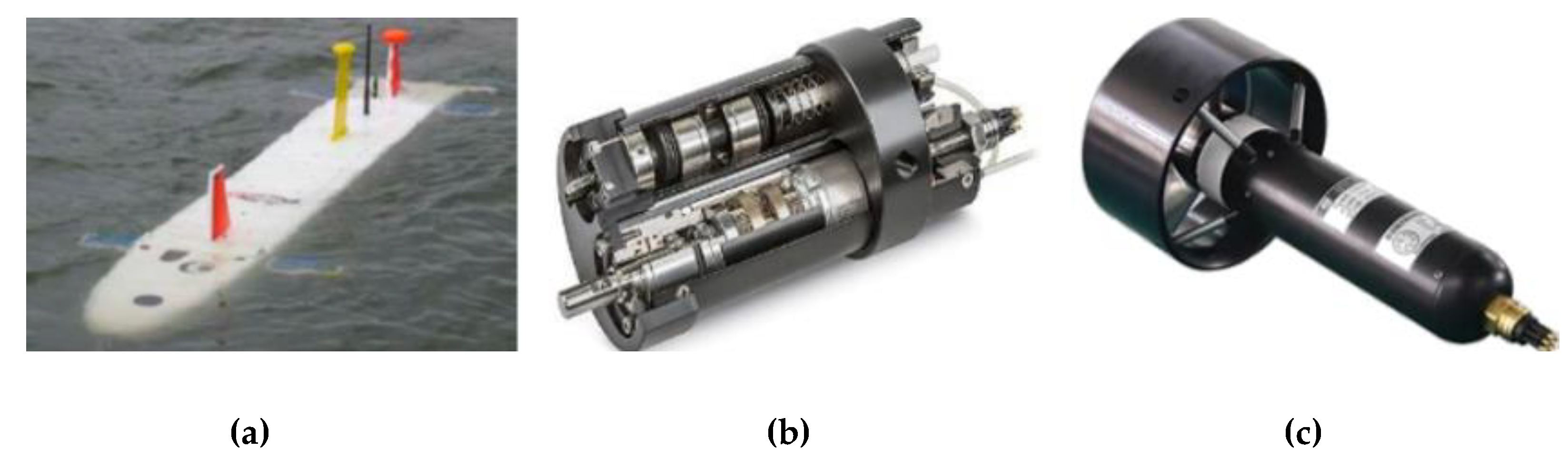
Figure 2.
The output signal for the control approaches with a 0.5-second step size. The black line represents the command signal. (a) Output signal obtained from deterministic artificial intelligence approach; (b) Output signal obtained from MF approach coupled with RLS estimation.
Figure 2.
The output signal for the control approaches with a 0.5-second step size. The black line represents the command signal. (a) Output signal obtained from deterministic artificial intelligence approach; (b) Output signal obtained from MF approach coupled with RLS estimation.
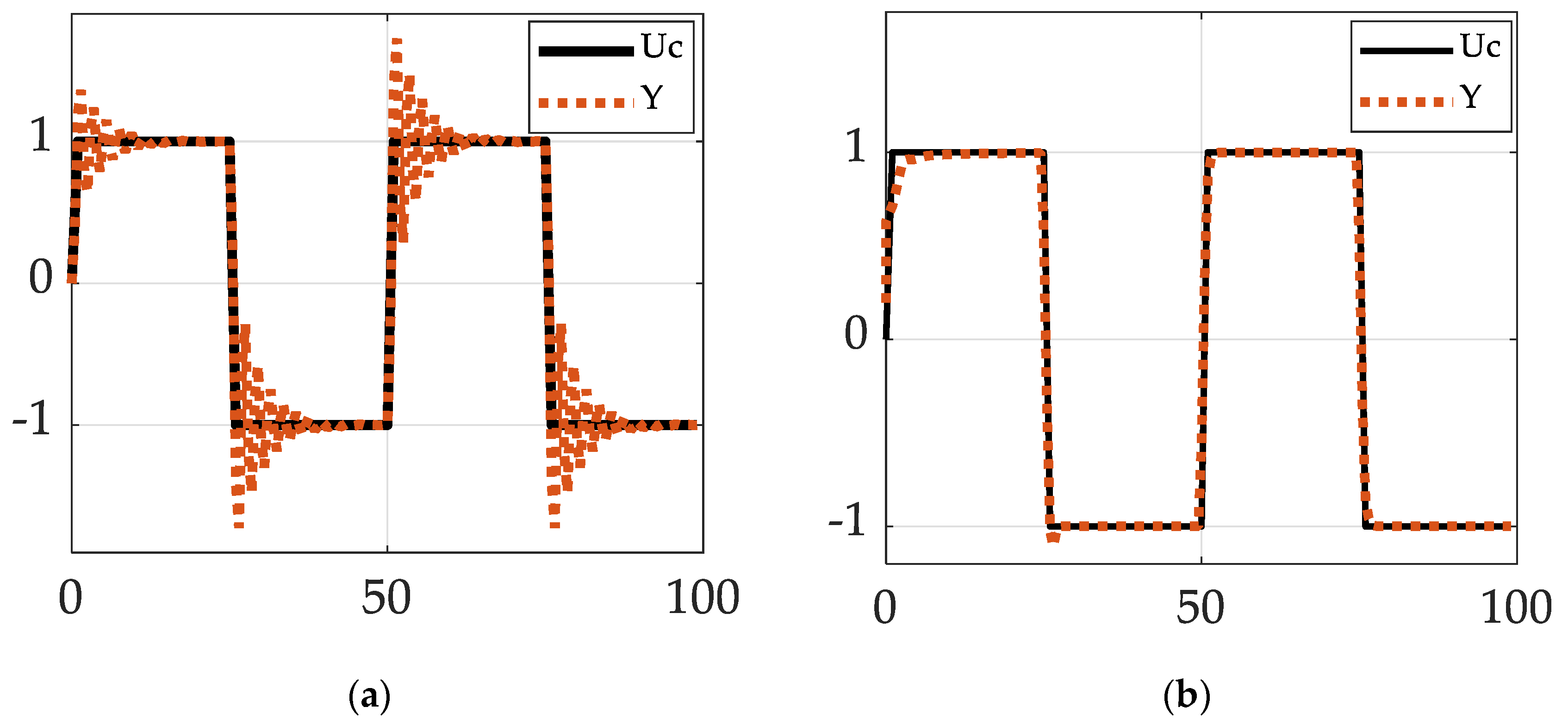
Figure 3.
The output signal for the deterministic artificial intelligence approaches with a 0.5-second step size. The black line represents the command signal. (a) Output signal obtained from discrete deterministic artificial intelligence approach; (b) Output signal generated from continuous deterministic artificial intelligence approach.
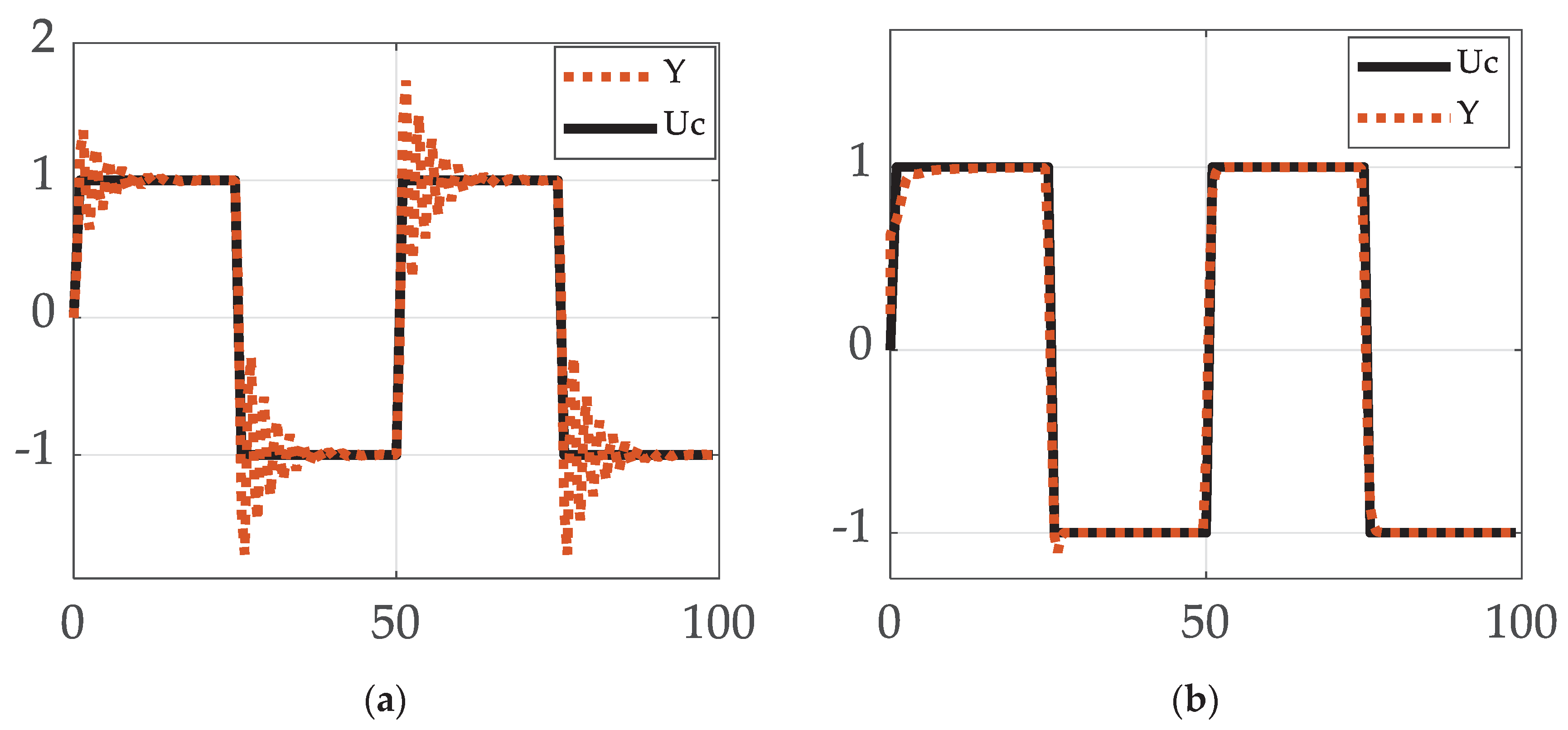

Table 1.
Error Distribution of comparison between Model Following Control (MF) and deterministic artificial intelligence with different step sizes.
Table 1.
Error Distribution of comparison between Model Following Control (MF) and deterministic artificial intelligence with different step sizes.
| Method | Step Size [seconds] |
Error Mean | Error Standard Deviation |
|---|---|---|---|
| Deterministic artificial intelligence | 0.60 | 6.3918 | 4.8100 |
| Model following | 0.60 | 0.0264 | 0.0973 |
| Deterministic artificial intelligence | 0.50 | 0.0956 | 0.1632 |
| Model following | 0.50 | 0.0277 | 0.0917 |
| Deterministic artificial intelligence | 0.27 | 0.0175 | 0.0545 |
| Model following | 0.27 | 0.0471 | 0.1745 |
| Deterministic artificial intelligence | 0.20 | 0.0114 | 0.0487 |
| Model following | 0.20 | 0.0608 | 0.2446 |
Table 2.
Error Distribution of comparison between Discrete deterministic artificial intelligence and Continuous deterministic artificial intelligence with different step sizes.
Table 2.
Error Distribution of comparison between Discrete deterministic artificial intelligence and Continuous deterministic artificial intelligence with different step sizes.
| Deterministic artificial intelligence Type | Step Size [sec] | Error Mean | Error Standard Deviation |
|---|---|---|---|
| Discrete | 0.50 | 0.0956 | 0.1632 |
| Continuous | 0.50 | 0.0223 | 0.1654 |
| Discrete | 0.20 | 0.0114 | 0.0487 |
| Continuous | 0.20 | 0.0122 | 0.1401 |
1 Integration solver step size matched to discretization interval.
Table 3.
Performance improvement with different step sizes.
| Method | Step Size [sec] | Error Mean | Error Standard Deviation |
|---|---|---|---|
| DAI | 0.60 | 6586% | 2847% |
| MF | 0.60 | -72% | -40% |
| DAI | 0.50 | 0% | 0% |
| MF | 0.50 | -71% | -44% |
| DAI | 0.27 | -82% | -67% |
| MF | 0.27 | -51% | 7% |
| DAI | 0.20 | -88% | -70% |
| MF | 0.20 | -36% | 50% |
1 Model following (MF) control and deterministic artificial intelligence (DAI).
Table 4.
Performance improvement for discrete and continuous deterministic artificial intelligence with different step sizes.
Table 4.
Performance improvement for discrete and continuous deterministic artificial intelligence with different step sizes.
| Deterministic artificial intelligence type | Step Size [sec] | Error Mean | Error Standard Deviation |
|---|---|---|---|
| Discrete | 0.50 | 0% | 0% |
| Continuous | 0.50 | -77% | 1% |
| Discrete | 0.20 | -88% | -70% |
| Continuous | 0.20 | -87% | -14% |
Disclaimer/Publisher’s Note: The statements, opinions and data contained in all publications are solely those of the individual author(s) and contributor(s) and not of MDPI and/or the editor(s). MDPI and/or the editor(s) disclaim responsibility for any injury to people or property resulting from any ideas, methods, instructions or products referred to in the content. |
© 2023 by the authors. Licensee MDPI, Basel, Switzerland. This article is an open access article distributed under the terms and conditions of the Creative Commons Attribution (CC BY) license (http://creativecommons.org/licenses/by/4.0/).
Copyright: This open access article is published under a Creative Commons CC BY 4.0 license, which permit the free download, distribution, and reuse, provided that the author and preprint are cited in any reuse.


