Reflection of Light as a Mechanical Phenomenon Applied to the Michelson Interferometer with Light from the Sun

1. Introduction

The Sun is a frame at relative rest in which sunlight travels at the emitted speed $c$. Earth travels at the revolving speed $v$ in this frame. The reflection of light as a mechanical phenomenon applies to the modified Michelson interferometer employed by Miller in his experiments with light from the Sun. Unlike the Tomaschek experiments, which use light from stars that may travel in the Universe at velocities different from that of the Sun, the fringe shifts in the Miller experiments are predictable. Based on Michelson’s derivation, Miller expected in his experiments at Mount Wilson a $1.12$ fringe shift and observed a fringe shift of $0.08$ in 1921 and $0.088$ in 1925. The reflection of light as a mechanical phenomenon predicts zero fringe shift for Miller’s experiment agreeing only with his observations at the Cleveland laboratory in 1924.

The reflection of light as a mechanical phenomenon [1,2,3] considers the speed of light independent from its moving source, but its reflection is similar to that of a ball by a wall in motion. This study continues with emission, propagation, and reflection of light as mechanical phenomena in inertial frames [4], observation of a star’s orbit [5], a general consideration of light reflection [6,7], and here with the reflection of light applied to the Miller experiment [8,9].

The emission, propagation, and reflection of light in inertial frames [4] conclude that physics phenomena in an inertial frame can be studied in any other inertial frame considered at relative rest. Here, the Sun’s frame at relative rest replaces the absolute frame for physics studies in Earth’s inertial frame. Thus, the Sun is a fixed light source for Earth, and Earth may be considered an inertial frame in the Sun’s frame at relative rest at the time of an experiment. The light from the Sun travels at the constant speed $c$ in any direction in the Sun’s frame at relative rest.

The reflection of light as a mechanical phenomenon applied to Michelson’s interferometer with a particular geometry [1,2] predicts zero fringe shift, and to a geometry [3] close to that presented in the Michelson-Morley experiment [10] offers $0.40\times {10}^{-4}$ fringe shift and greater for other geometries. Michelson’s derivation predicts a $0.40$ fringe shift.

This paper applies the theoretical derivation [1,2] and numerical calculation [3] to Miller’s experiments. Unlike the Tomaschek experiments [11], the fringe shifts in Miller’s experiments are predictable.

The reflection of light as a mechanical phenomenon [1,2,5] based on the elastic collision of balls with a wall in motion at the limit when the mass of balls converges to zero offers the equation

$$c_{ra}=c_s+v_i+v_r.$$

(1)

In Eq. (1), $c_{ra}$ is the speed of a reflected wavefront of a ray of light by a mirror in motion, $c_s$ is the wavefront speed from the source or a mirror as a source, $v_i$ is the mirror speed in the opposite direction of the incident wavefront from the source, and $v_r$ is the mirror speed in the direction of the reflected wavefront. Here, these speeds are in the Sun’s frame at relative rest. The mirror moves in one unique observable direction with speed $v$. However, regarding the light wavefront, as far as the collision effect is concerned, it has multiple directions of $v_i$ and $v_r$ at the moment of collision according to the mirror inclinations. Speeds $v_i$ and $v_r$ are projections of $v$ in their corresponding directions.

Another form of Eq. (1) is

$$c_{ra}=c_s+v\cos a+v\cos b.$$

(2)

In Eq. (2), the speeds $v\cos a$ and $v\cos b$ replace $v_i$ and $v_r$ in Eq. (1), respectively. Angle $a$ corresponds to the opposite direction of the incident wavefront, and angle $b$ to the direction of the reflected wavefront. These angles are measured from the direction of velocity vector $v$, originating at the point of collision. The directions

of $v_i$ and $v_r$ are outward from the point of collision.

In the Sun’s frame at relative rest, the velocity of mirrors attached to the Michelson interferometer is affected by Earth’s revolving velocity $v$ around the Sun and Earth’s spin velocities $u$. Therefore, Eq. (1) becomes the equation

$$c_{ra}=c_s+\left(v_i+u_i\right)+\left(v_r+u_r\right),$$

(3)

and Eq. (2) the equation

$$c_{ra}=c_s+\left(v\cos a_v+u\cos a_u\right)+\left(v\cos b_v+u\cos b_u\right),$$

(4)

where $a_v$, $a_u$, $b_v$, and $b_u$ are the corresponding angle for the incident and reflected wavefront of light for velocity $v$ and $u$.

Michelson [10] derives the fringe shift in the space filled with ether. Consequently, the speed of light from a source before and after reflection is the constant $c$. The study of light reflection as a mechanical phenomenon [1,2,5] occurs in a vacuum. Like a ball in an elastic collision with a wall, the wavefront speed changes after reflection by a moving mirror. Therefore, the difference between these two approaches is the reflection of light by a moving mirror.

2. Interferometer on Earth’s Equator

2.1. General considerations

The following drawings illustrate a way to bring the light from the Sun to a modified Michelson interferometer. For simplicity, Earth’s axis has no tilt.

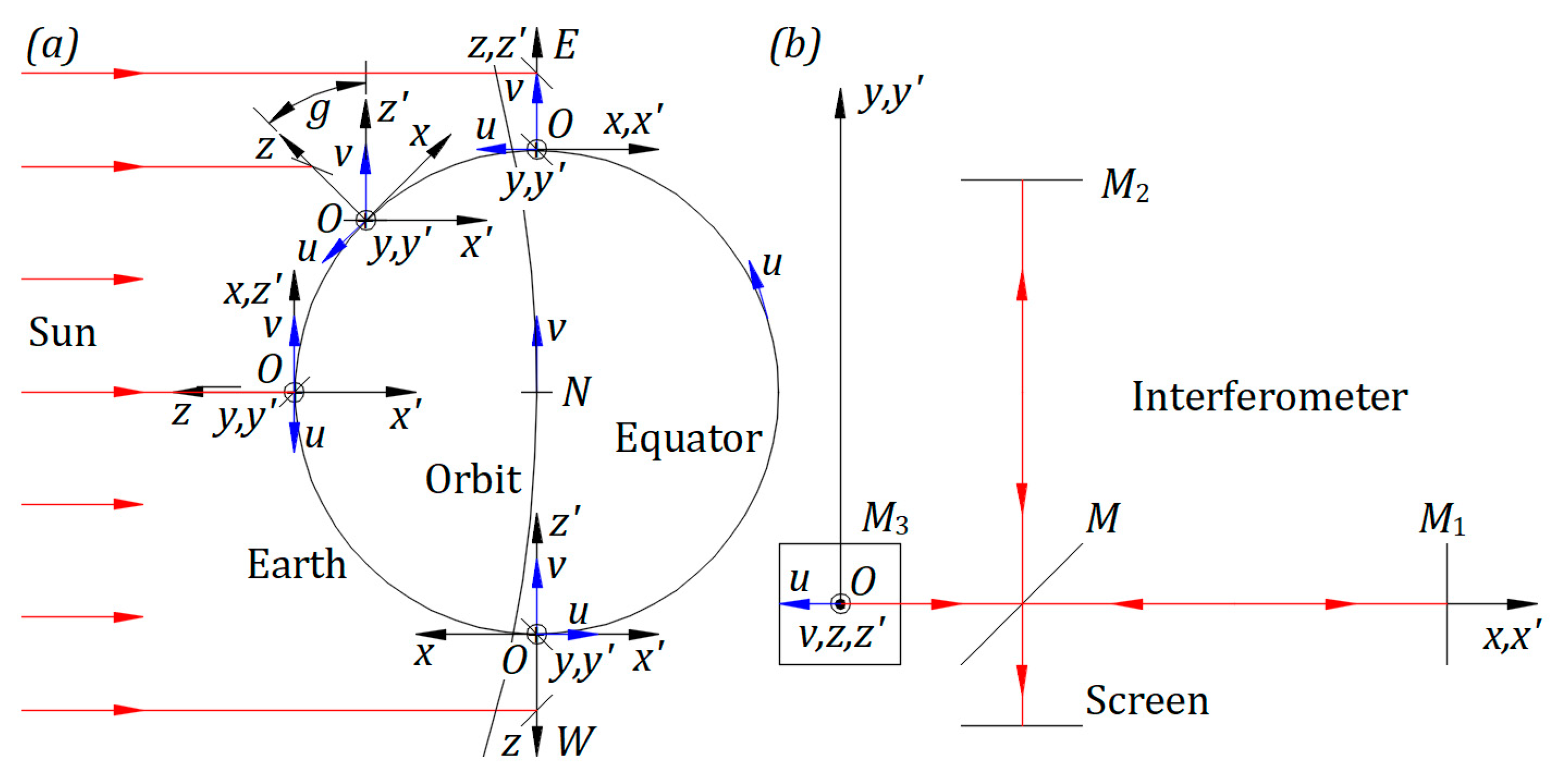
Figure 1a illustrates Earth’s equatorial circle, Earth’s revolving orbit around the Sun, and the center of the Sun and Earth in the same plane. The North Pole is outward, and the South Pole is inward, perpendicular to the paper plane.

An observer in the Sun’s frame at relative rest also perceives the physics phenomena as a local observer in Earth’s inertial frame. The observer’s location is on the North side of the Equator.

Figure 1b illustrates the Michelson interferometer at 6 am, as seen from the top side of Figure 1a. Mirrors $M_1$, $M_2$, $M_3$, and beam splitter $M$ belong to the instrument. Mirror $M_3$ replaces the instrument’s source of light.

The cartesian frame $Oxyz$, fixed to the instrument, originates at point $O$ of $M_3$. Axis $Ox$ is on the horizontal line, and axis $Oz$ is perpendicular to Earth’s local surface. Plane $Oxy$ is parallel to Earth’s local surface and perpendicular to the local Earth’s radius at point $O$. At 6 am, the revolving velocity $v$ of Earth coincides with $Oz$.

The interferometer is in plane $Oxy$. It rotates counterclockwise around $Oz$ with an angle $f$ measured from $Ox$. The initial position of the instrument is when direction $O{M}_1$ coincides with $Ox$ for $f=0°$, as shown in Figure 1b.

In the Sun’s frame at relative rest, a vector velocity $v$ in the direction $Oz’$ of the cartesian frame $Ox’y’z’$ is attached permanently to the origin $O$ of $Oxyz$. Earth’s spin changes the origin position $O$ of $Oxyz$ and $Ox’y’z’$; different from $Oxyz$, $Ox’y’z’$ keeps its axes’ directions fixed in the Sun’s frame at relative rest.

The instrument on the Equator belongs to a local Meridian. The Equator’s start position can be defined when: the local Meridian of the instrument is at 6 am, frames $Oxyz$ and $Ox\mathrm{’}y\mathrm{’}z\mathrm{’}$ coincide, and the device is at the initial position, as illustrated in Figure 1b.

Figure 1. (a) Interferometer on Earth’s Equator at 6 am, noon, 6 pm, and between 6 am and 6 pm. (b) Interferometer details.

Figure 1. (a) Interferometer on Earth’s Equator at 6 am, noon, 6 pm, and between 6 am and 6 pm. (b) Interferometer details.

In the Sun’s frame at relative rest, the center of the Sun, Earth’s orbit, and the Equator’s circle are always in the same plane. Planes $Oxz$ and $Ox\mathrm{’}z\mathrm{’}$ belong to Equator’s plane. Plane $Oxy$ is parallel to Earth’s local surface and perpendicular to Equator’s plane. Axes $Oy$ and $Oy\mathrm{’}$ are overlapping from 6 am to 6 pm.

Earth’s spin changes the position of $Oxyz$. At the same time, in plane $Oxz$, axis $Oz\mathrm{’}$ rotates clockwise around $Oy\mathrm{’}$, keeping the directions of $Ox\mathrm{’}y\mathrm{’}z\mathrm{’}$ unchanged. $Oz\mathrm{’}$ with the vector velocity $v$ at $O$ makes the angle $g$ measured from $Oz$.

Figure 1a indicates the position of the interferometer at 6 am, which is the Equator’s start position, corresponding to $g=0°$. Earth’s spin brings the interferometer to an angle $g$ between 6 am and 6 pm, to $g=90°$ at noon, and $g=180°$ at 6 pm.

2.2. Interferometer on the Equator at 6 am, noon, and 6 pm

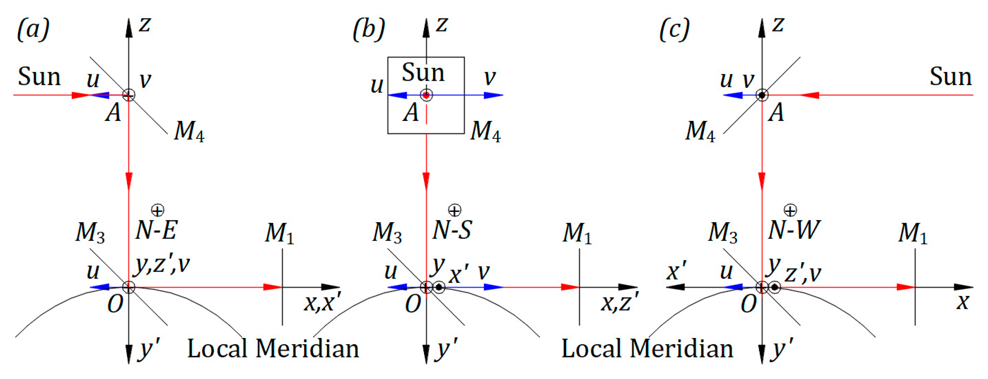
Figure 2a depicts the Equator’s start position at 6 am for $g=0°$. Earth’s spin brings the interferometer at noon, as illustrated in Figure 2b for $g=90°$, at 6 pm, as presented in Figure 2c for $g=180°$, and in general, at a time between 6 am and 6 pm, as shown in Figure 3a for an angle $g$.

Point $A$ belongs to mirror $M_4$ and to axis $Oz$. Mirror $M_4$, axis $Oz$, mirror $M_3$, and interferometer form a solid structure. Mirror $M_4$ rotates at the Equator around an axis through point $A$ perpendicular to $Oxz$. At the North Pole around axis $Oz$. And between the Equator and the North Pole around both. $M_4$ stays fixed while the interferometer rotates $360°$ around axis $Oz$.

Considering that the Sun emits parallel rays of light in the direction from the Sun’s center toward Earth’s center, only these rays are reflected by $M_4$ in the opposite direction to $Oz$ toward $M_3$. The incident rays from the Sun are perpendicular to $v$ at any location on Earth.

Figure 2. Interferometer on the Equator: (a) at 6 am, (b) at noon, and (c) at 6 pm.

Figure 2. Interferometer on the Equator: (a) at 6 am, (b) at noon, and (c) at 6 pm.

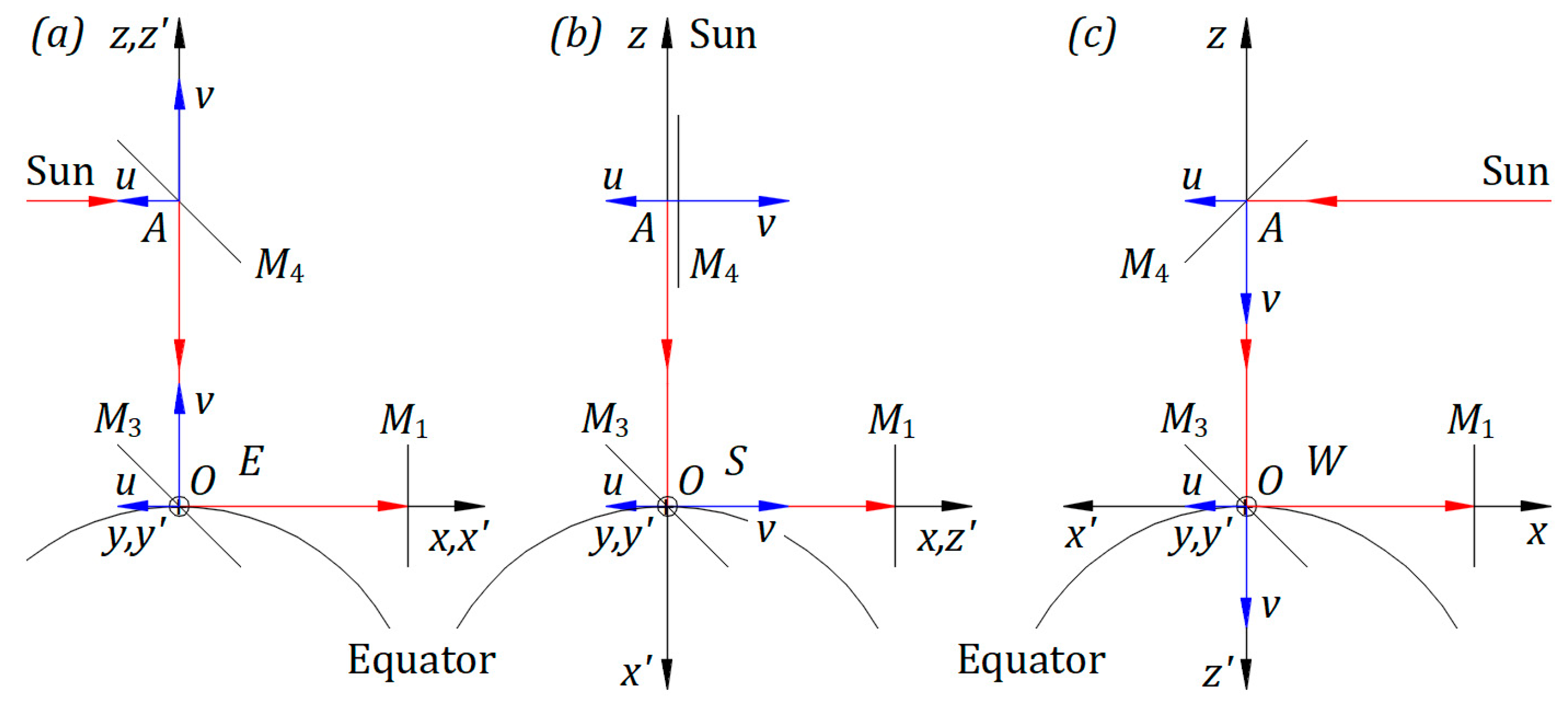
The vector sum of velocity $v$ and $u$ offers the moving velocity of the device in the Sun’s frame at relative rest. The instrument has a longitudinal velocity given by velocities $v$ and $u$ and a transversal velocity only given by velocity $v$ at any Earth’s location.

In Figure 2a, point $A$ of $M_4$ reflects the ray of light toward $O$ with the speed $c_{ra}$ given by Eq. (4), $c_{ra}=c_s+\left(v\cos a_v+u\cos a_u\right)+$  $\left(v\cos b_v+u\cos b_u\right)=c+$  $\left(v\cos 90°+u\cos 0°\right)+\left(v\cos 180°+u\cos 90°\right)=$  $c+u-v$.

The ray reflected at $O$ along $Ox$ and $O{M}_1$ for $f=0°$ has the speed $c_{f=0°}=c_s+\left(v\cos a_v+u\cos a_u\right)+\left(v\cos b_v+u\cos b_u\right)$. With $c_s=c_{ra}$, $c_{f=0°}=\left(c+u-v\right)+\left(v\cos 0°+u\cos 90°\right)+\left(v\cos 90°+u\cos 180°\right)=c$.

The projection of $v$ on $Oz$ is $v_z=v$. The rays reflected by $M_3$ drift transversal opposite to velocity $v_z$.

In Figure 2b, the light from the Sun travels perpendicular to $Ox$; therefore, no need for mirror $M_4$. At this position, $M_4$ rotates $180°$ around $Oz$ to continue reflecting rays for $90°<g\le 180°$.

The ray reflected at $O$ along $Ox$ and $O{M}_1$ for $f=0°$ has, according to Eq. (4), the speed $c_{f=0°}=c_s+$  $\left(v\cos a_v+u\cos a_u\right)+\left(v\cos b_v+u\cos b_u\right)=c+\left(v\cos 90°+u\cos 90°\right)$  $+\left(v\cos 0°+u\cos 180°\right)=c+v-u$.

The projection of $v$ on $Oz$ is zero. Thus, there is no transversal drift on rays reflected at $M_3$.

Figure 2c shows the device at 6 pm. Point $A$ of $M_4$ reflects the ray of light toward $O$ with the speed $c_{ra}$ given by Eq. (4), $c_{ra}=c_s+\left(v\cos a_v+u\cos a_u\right)+\left(v\cos b_v+u\cos b_u\right)=c+$  $\left(v\cos 90°+u\cos 180°\right)$  $+\left(v\cos 0°+u\cos 90°\right)=c-u+v$.

The ray reflected at $O$ along $Ox$ and $O{M}_1$ for $f=0°$ has the speed $c_{f=0°}=c_s+\left(v\cos a_v+u\cos a_u\right)+\left(v\cos b_v+u\cos b_u\right)=c_{ra}+\left(v\cos 180°+u\cos 90°\right)$  $+(v\cos 90°+u\cos 180°)=$  $\left(c-u+v\right)-v-u=c-2u$.

The projection of $v$ on $Oz$ is $v_z=-v$. The rays reflected by $M_3$ drift transversal opposite to velocity $v_z$.

2.3. Interferometer on the Equator at an angle g

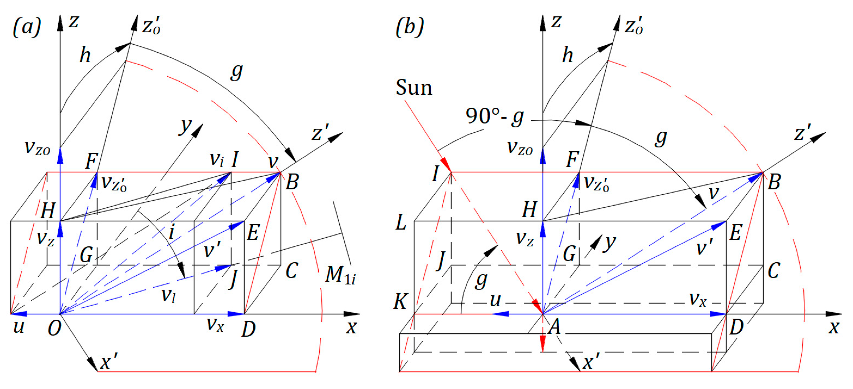
Figure 3a presents the instrument between 6 am and 6 pm when $Oz\mathrm{’}$ makes an angle $g$ measured from $Oz$. To reflect the rays in the direction $AO$, $M_4$ rotates around the axis through point $A$ and perpendicular to $Oxz$. Angle $g$ has an opposite direction to Earth’s spin.

From 6 am to 6 pm for $0°\le g\le 180°$, projection of $v$ on $Oz$ is the transversal speed of the instrument in the Sun’s frame at relative rest

$$v_z=v\cos g$$

(5)

Projection of $v$ on $Ox$, $v_x=v\cos (90°-g)$, offers the equation

$$v_x=v\sin g.$$

(6)

Figure 3. (a) Interferometer at an angle $g$. (b) Three-dimensional detail of mechanical velocities at point $O$. (c) Interferometer at an angle $f$ from $Ox$ illustrated in plane $Oxy$.

Figure 3. (a) Interferometer at an angle $g$. (b) Three-dimensional detail of mechanical velocities at point $O$. (c) Interferometer at an angle $f$ from $Ox$ illustrated in plane $Oxy$.

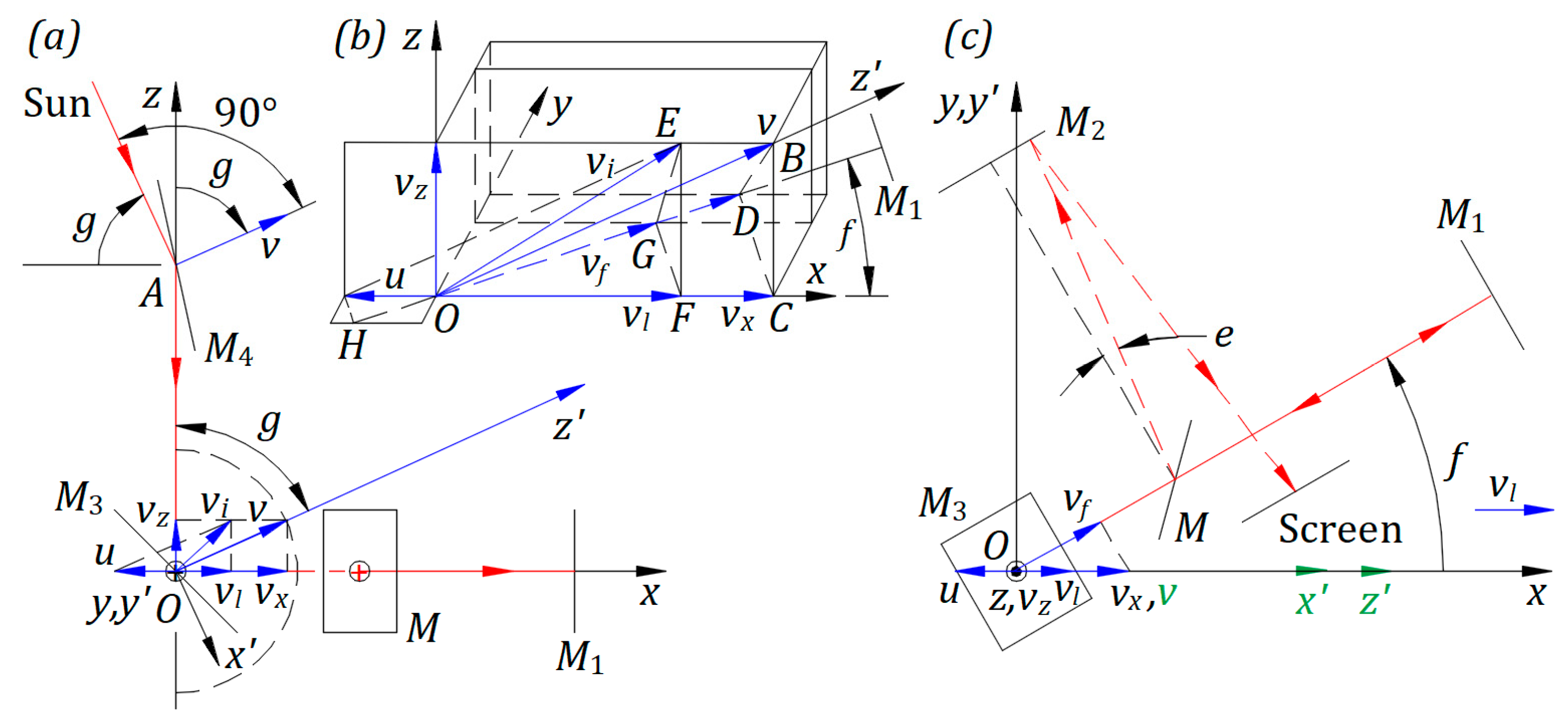
In Figure 3b, the vector sum of velocities $v$ and $u$, shown in the plane $Oxz$, is the moving velocity $v_i$ of the device in the Sun’s frame at relative rest. $CF$ and $BE$ are equal to $u$ for any angle $g$. The projection of $v$ and $v_i$ are $v_x$ and $v_l$, respectively. $v_l$ is the longitudinal component of velocity $v$ for the instrument.

$BD$ and $EG$ are perpendicular to $O{\mathrm{M}}_1$ for any angle $f$. $OBC$ and $BCD$ planes and their intersection along $BC$ are perpendicular to $Oxy$, and $BD$ is perpendicular to $OD$. Therefore, $OD$ is perpendicular to plane $BCD$, and $CD$ is perpendicular to $OD$. Thus, the projections of $v$ and $v_x$ on $O{\mathrm{M}}_1$ are identical to $OD=v_x\cos f$. With the same reasoning, the projections of $v_i$ and $v_l$ on $O{M}_1$ are identical to $OG=v_f=v_l\cos f$. Point $O$ belongs to $DH$, and $DG=OH$ that vary with angle $g$.

The longitudinal speed of the instrument in the Sun’s frame at relative rest $v_l=v_x+u\cos 180°$ then, with $v_x$ from Eq. (6),

$$v_l=v\sin g-u.$$

(7)

Figure 3c illustrates the top side view of Figure 3a with the interferometer rotated by an angle $f$ from $Ox$. For the geometry presented in Ref. [3], reflected rays by beam splitter $M$ travel as illustrated at an angle $e$ from the perpendicular line to $M_2$. $Ox’$, $Oz’$, and $v$ in green indicate that they are not in plane $Oxy$.

Point $A$ of $M_4$ reflects the ray of light toward $O$ with the speed $c_{ra}=c_s+$  $\left(v\cos a_v+u\cos a_u\right)+$  $\left(v\cos b_v+u\cos b_u\right)=$  $c+\left(v\cos 90°+u\cos g\right)+$  $\left(v\cos (180°+g)+u\cos 90°\right)$ that gives the equation

$$c_{ra}=c+u\cos g-v\cos g.$$

(8)

The ray from $A$ reflected at $O$ along $Ox$, employing Eq. (4), has the speed $c_{f=0°}=c_{ra}+\left(v\cos a_v+u\cos a_u\right)+\left(v\cos b_v+u\cos b_u\right)$. The term $\left(v\cos a_v+u\cos a_u\right)$ is according to Figure 3a,b, and $\left(v\cos b_v+u\cos b_u\right)=v_l$ given by Eq. (7). With $c_{ra}$ from Eq. (8), $c_{f=0°}=\left(c+u\cos g-v\cos g\right)+\left(v\cos g+u\cos 90°\right)+v_l$ yields the equation

$$c_{f=0°}=c+u\cos g+v_l.$$

(9)

With the same reasoning as for $c_{f=0°}$, the reflected speed of light at $O$ along $O{M}_1$ at an angle $f$ is $c_f=c_{ra}+$  $\left(v\cos a_v+u\cos a_u\right)+$  $\left(v\cos b_v+u\cos b_u\right)=$  $\left(c+u\cos g-v\cos g\right)+$  $\left(v\cos g+u\cos 90°\right)+v_l\cos f$ that offers the equation

$$c_f=c+u\cos g+v_l\cos f.$$

(10)

3. Interferometer on the North Pole

The solid structure, illustrated in Figure 2a, brought from the Equator at 6 am along the local Meridian at the North Pole, looks like in Figure 4a. From the Equator to the North Pole, the frame $Oxyz$ rotates $90°$ in the Sun’s frame at relative rest. In plane $Oyz$, $Oz\mathrm{’}$ rotates $90°$ around $Ox\mathrm{’}$ from $Oz$ to $Oy$; after rotation, $Oz\mathrm{’}$ has the same direction as $Oy$. Planes $Oxy$ and $Ox\mathrm{’}z\mathrm{’}$ coincide and are parallel to Equator’s plane. Axis $Oy\mathrm{’}$ is perpendicular to Equator’s plane.

Earth’s spin rotates $Oxyz$ in the Sun’s frame at relative rest. In plane $Oxy$, $Oz\mathrm{’}$ rotates around fixed $Oy\mathrm{’}$ from $Oy$ at 6 am at angle $g=0°$, as illustrated in Figure 4a, to $Ox$ at noon at angle $g=90°$, as in Figure 4b, and to $-Oy$ at 6 pm at angle $g=180°$, as in Figure 4c. At the North Pole, mirror $M_4$ rotates only around $Oz$.

4. Interferometer on a Latitude

The right side view of Figure 2a, ignoring $M_1$, is as in Figure 5a. Moving the solid structure from the Equator toward the North Pole, $Oxyz$ rotates in the Sun’s frame at relative rest. Velocity $v$ with its axis $Oz’$ rotates in plane $Oyz$ around $Ox’$ with angle $h$ measured from axis $Oz$, as visualized in Figure 5b. For $h=0°$, the interferometer is at the Equator, and for $h=90°$ at the North Pole. In the rotation on a Meridian, from the Equator to the North Pole, Mirror $M_4$ stays fixed.

In Figure 5b, we can define the Latitude’s start position at the intersection of the local Meridian with the local Latitude at 6 am. $Oz’$ is marked with index o for angle $g$ $=0°$, $O{z}_{\mathrm{o}}^{’}$, and is in plane $Oyz$ making an angle $h$ measured from $Oz$.

Plane $Ox’z’$ is parallel, and axis $Oy’$ is perpendicular to Equator’s plane here and at any location on Earth. Plane $Oxy$ is parallel, and the axis $Oz$ is perpendicular to Earth’s local surface as on any place on Earth. $Oxz$ and $Ox’z’$ are perpendicular to plane $Oyz$ and intersect along $Ox$.

Earth’s spin rotates the frame $Oxyz$ on the Latitude from 6 am to 6 pm. At the same time, velocity $v$ with its axis $Oz’$ rotates around fixed axis $Oy’$ from $O{z}_{\mathrm{o}}^{’}$ at 6 am for angle $g=0°$ to $Ox$ at noon for $g=90°$ and to $-O{z}_{\mathrm{o}}^{’}$ at 6 pm for $g=180°$. Thus, on a Meridian, angle $g$ is identical when the instrument is on different Latitudes to that at the Equator. On a Latitude, mirror $M_4$ rotates around both axes to capture the parallel rays from the Sun.

The view from the opposite direction of $Oy\mathrm{’}$ shows vector $v$ with its axis $Oz\mathrm{’}$ rotating from 6 am to 6 pm on a semicircle with origin at $O$ and radius $v$. The semicircle is in plane $Ox\mathrm{’}z\mathrm{’}$. Any angle $h$ yields an identical image. The semicircle is identical to that in Figure 3a, illustrated in a dashed line in plane $Oxz$.

The view from the opposite direction of $Oy$ sees the semicircle projection of the vector $v$ as a semi-ellipse in plane $Oxz$, illustrated in a dashed line in Figure 5c. The projection points of this semi-ellipse on $Oz$ represent the speeds $v_z$ for angles $g$.

Figure 5c is the left side view of Figure 5b for an angle $g$ measured from $O{z}_{\mathrm{o}}^{\mathrm{’}}$. The projection of the velocity $v$ that belongs to $Oz\mathrm{’}$ on plane $Oxz$ is $v\mathrm{’}$. $Ox\mathrm{’}$, $Oy\mathrm{’}$, and $Oz\mathrm{’}$ axes are depicted in green to indicate that they are not in plane $Oxz$; $Ox\mathrm{’}$ is in the front, and $Oy\mathrm{’}$ and $Oz\mathrm{’}$ are in the back of plane $Oxz$.

Figure 5. (a) Interferometer on the Equator at 6 am. Interferometer on a Latitude: (b) at angle $h$, and (c) left side view of Figure 5(b).

Figure 5. (a) Interferometer on the Equator at 6 am. Interferometer on a Latitude: (b) at angle $h$, and (c) left side view of Figure 5(b).

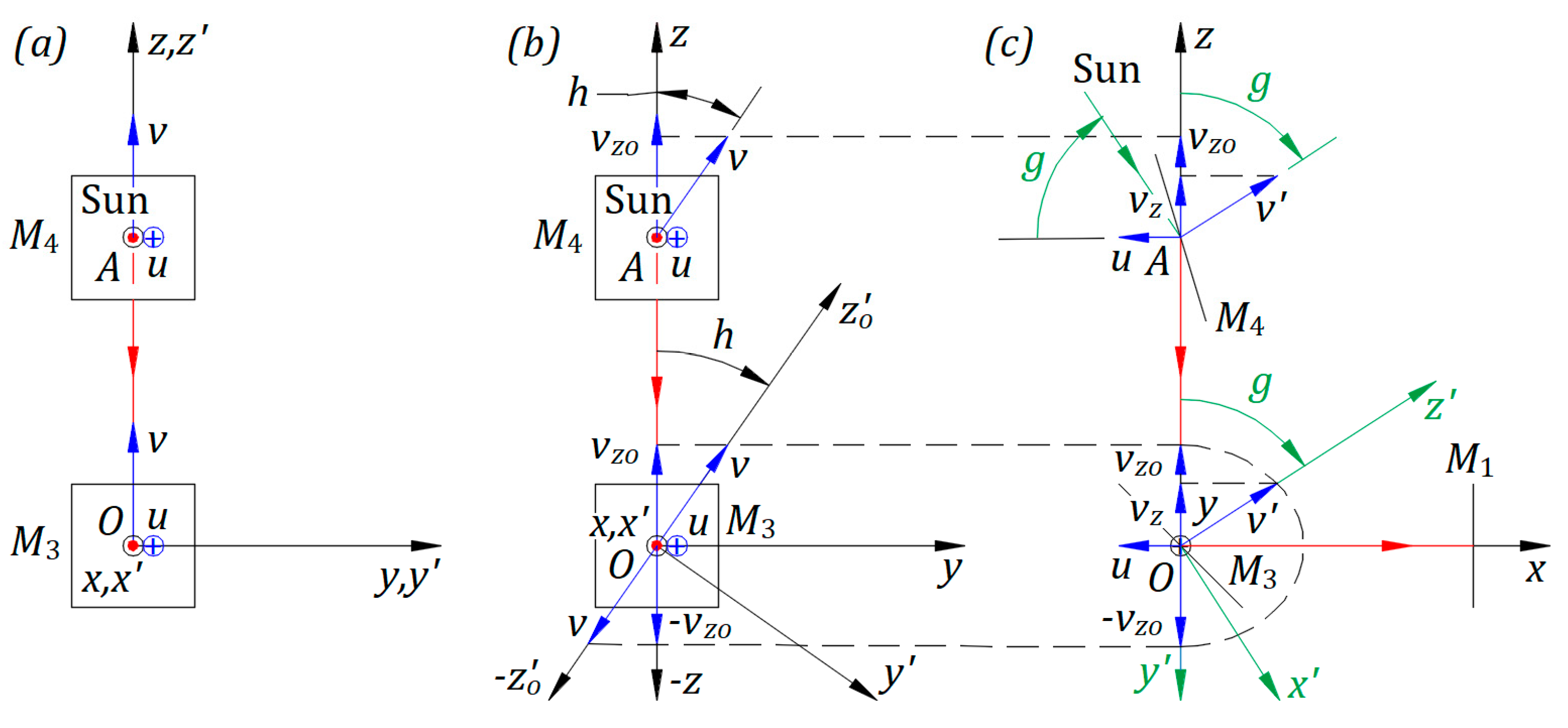
Planes $Oxz$ and $Ox\mathrm{’}z\mathrm{’}$ intersect along $Ox$. $Ox\mathrm{’}$ coincides with $Ox$ at $g=0°$. Axis $Oz\mathrm{’}$ rotates in the back of plane $Oxz$ from $O{z}_{\mathrm{o}}^{\mathrm{’}}$ at the Latitude’s start position when it is behind $Oz$ for $g=0°$ to plane $Oxz$ coinciding with $Ox$ for $g=90°$. Then $Oz\mathrm{’}$ rotates in front of plane $Oxz$ to $-O{z}_{\mathrm{o}}^{\mathrm{’}}$ for $g=180°$, above $-Oz$. $Ox\mathrm{’}$ rotates in front of plane $Oxz$ from $Ox$ for $g=0°$ to above $-Oz$ for $g=90°$, then to $-Ox$ for $g=180°$.

Figure 6a offers a three-dimensional visualization of the mechanical velocities at point $O$ of Figure 5c. Axis $O{z}_{\mathrm{o}}^{\mathrm{’}}$ is in plane $Oyz$. Rectangular $ODEH$ belongs to $Oxz$, $ODCG$ to $Oxy$, and $OGFH$ to $Oyz$. The speed $v$ is along axis $Oz\mathrm{’}$. Index $i$ for ${\mathrm{M}}_{1i}$ indicates that mirror $M_1$ location corresponds to angles $i$ defined below. Velocities $v$, $v_i$, and $v_{z_{\mathrm{o}}^{\mathrm{’}}}$ belong to rectangular $ODBF$ of the plane in red; $v_x$ and $v_l$ to plane $Oxy$.

The projection of $v$ on $Oz$ at the Latitude’s start position offers the equation

$$v_{z\mathrm{o}}=v\cos h.$$

(11)

The projection of $v$ on $O{z}_{\mathrm{o}}^{\mathrm{’}}$ is $OF=v_{z_{\mathrm{o}}^{\mathrm{’}}}$, therefore,

$$v_{z_{\mathrm{o}}^{\mathrm{’}}}=v\cos g.$$

(12)

The projection of $v_{z_{\mathrm{o}}^{\mathrm{’}}}$ on $Oz$, $v_z=v_{z_{\mathrm{o}}^{\mathrm{’}}}\cos h$, is also the projection of $v$ on $Oz$. Employing Eq. (12),

$$v_z=v\cos g\cos h.$$

(13)

Figure 6. Mechanical velocities of Figure 5(c): (a) at point $O$ and (b) at point $A$.

Figure 6. Mechanical velocities of Figure 5(c): (a) at point $O$ and (b) at point $A$.

The contribution of $u$ on $Oz$ is zero at all times; therefore, $v_z$ is the transversal speed of the instrument in the Sun’s frame at relative rest.

$Ox$ belongs to $Ox’z’$ as well. The projection of $v$ on $Ox$ is $v_x=v\cos (90°-g)$, therefore,

$$v_x=v\sin g$$

(14)

The vector sum of velocities $v$ and $u$ is the instrument velocity in the Sun’s frame at relative rest $v_i$. Angle $OBF=BOD=\cos (90°-g)$ and from triangle $OBI$, the law of cosines yields the magnitude of velocity $v_i=\sqrt{v^2-2vu\cos (90°-g)+u^2}$ that yields the equation

$$v_i=\sqrt{v^2-2vu\sin g+u^2}.$$

(15)

The projection of $v_i$ on $Oz$ also is $v_z$ from Eq. (13). The triangle $OIJ$ gives the projection of $v_i$ on the plane $Oxy$, $v_l$, that is the longitudinal speed of the interferometer in the Sun’s frame at relative rest. $IJ=OH$, then

$$v_l=\sqrt{v_i^2-v_z^2}.$$

(16)

$GJ=BF-BI=v_x-u$, then in triangle $OGJ$, $\sin i=\left(v_x-u\right)/v_l$ that offers the equation

$$i={\sin }^{-1}\left[\left(v_x-u\right)/v_l\right].$$

(17)

Angle $i$ indicates $O{\mathrm{M}}_1$ direction at the initial position, $O{\mathrm{M}}_{1i}$, when $O{\mathrm{M}}_1$ direction coincides with that of $v_l$.

Figure 6b offers a three-dimensional visualization of the mechanical velocities at point $A$ of Figure 5c. At $A$, we can attach the same frame as at $O$, $Axyz$, and $Ax\mathrm{’}y\mathrm{’}z\mathrm{’}$. Axis $A{z}_0^{\mathrm{’}}$ is in plane $Ayz$. Velocities $v$ and $v_{z_{\mathrm{o}}^{\mathrm{’}}}$ belong to rectangular $BDKI$ of plane $Ax\mathrm{’}z\mathrm{’}$, which contains red lines. The ray from the Sun travels in this plane along the line $IA$. Point $A$ of $M_4$ reflects it towards $O$. $M_4$ must be adjusted with both axes to reflect the incident ray along axis $Ax\mathrm{’}$ from I to A towards $O$.

The ray of light reflected at $A$ toward $O$ has the speed $c_{ra}=c_s+\left(v\cos a_v+u\cos a_u\right)+$  $\left(v\cos b_v+u\cos b_u\right)=$  $c+\left(v\cos 90°+u\cos g\right)$  $+\left(-v_z+u\cos 90°\right)$ that gives the equation

$$c_{ra}=c+u\cos g-v_z.$$

(18)

From Figure 6a, we can calculate the speed of light reflected in the direction ${\mathrm{M}}_{1i}$ for angle $i$, $c_i=c_{ra}+\left(v\cos a_v+u\cos a_u\right)+\left(v\cos b_v+u\cos b_u\right)$. $v_l$ from Eq. (16) includes both $v$ and $u$ contributions along $O{\mathrm{M}}_{1i}$. Thus, term $\left(v\cos b_v+u\cos b_u\right)=v_l$, and then $c_i=\left(c+u\cos g-v_z\right)+\left(v_z+u\cos 90°\right)+v_l$ that offers the equation

$$c_i=c+u\cos g+v_l$$

(19)

For the same reason as in Figure 3b, the projections of $v_i$ and $v_l$ on $O{\mathrm{M}}_1$ are identical for any angle $f$ measured from ${\mathrm{M}}_{1i}$. The speed of light reflected at $O$ in the direction of $O{\mathrm{M}}_1$ for an angle $f$ measured from ${\mathrm{M}}_{1i}$ is $c_{if}=c_{ra}+\left(v\cos a_v+u\cos a_u\right)+\left(v\cos b_v+u\cos b_u\right)=\left(c+u\cos g-v_z\right)+\left(v_z+u\cos 90°\right)+v_l\cos f$ that yield the equation

$$c_{if}=c+u\cos g+v_l\cos f$$

(20)

5. Numerical calculation of the fringe shift

For the length $L=32$ m of the interferometer’s arms, Miller expected a $1.12$ fringe shift based on Michelson’s derivation [10] and observed, at Mount Wilson, $0.08$ in 1921 and $0.088$ in 1925 [8,9]. The observations taken in the laboratory at Cleveland 1924, with sunlight and laboratory sources, show a null result of experiments. The above discrepancy in experimental results requires a theory to support it or a reevaluation of Miller’s experiments.

The velocity $v$ is the moving velocity of the instrument in the Sun’s frame at relative rest. The device has the longitudinal velocity $v_x$ at the Equator and $v_l$ on a Meridian parallel to and the transversal velocity $v_z$ perpendicular to plane $Oxy$. To correctly calculate the fringe shift within the interferometer, we have to consider both velocities, but there is no such theoretical derivation.

In the following derivation, we assume that the fringe shift is not affected by the transversal speed $v_z$, and we calculate the fringe shift for the four positions offered by Ref. [3].

The numerical calculation can be performed on a spreadsheet according to the theoretical derivation of Ref. [3], starting with the set of speeds $c_{11}$, $c_{12}$, $c_{13}$, $c_{21}$, and $c_{22}$, followed by the times the light travels its paths and their differences, and finally, the fringe shift for each of the four positions at angle $a=0°$, $90°,180°$, and $270°$.

The initial position of the interferometer for $f=0°$ corresponds to the $a=180°$ position in Ref. [3] because between the two selected initial positions, there is a difference of $180°$. Thus, for $f=0°$, $90°$, $180°$, and $270°$ positions correspond to $a=180°$, $270°$, $0°$, and $90°$ positions in Ref. [3].

The speed $c_{if}$ from Eq. (20) replaces the speed $c$ correspondingly in the sets of speeds $c_{11}$, $c_{12}$, $c_{13}$, $c_{21}$, and $c_{22}$ in the four positions as defined in Ref. [3]. The numerical magnitude of speed $v_l$ from Eq. (16) replaces speed $v$ in all four positions of Ref. [3], including the above sets of speeds.

In Ref. [3], rays along the screen interfere because their speeds, $c_{13}$ and $c_{22}$, are equal. Ref. [3] derives the difference between the two light paths in the number of wavelengths $N_{\mathrm{1,2},3,4}=c∆t_{\mathrm{1,2},\mathrm{3,4}}/\lambda$, where $∆t_{\mathrm{1,2.3}.4}=t_2-t_1$ for each of the four positions. $∆t_{\mathrm{1,2.3}.4}$ is the difference in the time the two rays travel their paths with the same or different speeds. $c$ is the constant $3\times {10}^8$ m/s and $\lambda$ the wavelength of light for constant $c$.

If the speed of the two interfering rays increases or decreases, their wavelengths increase or decrease directly proportional. Therefore, the ratio speed/wavelength is a constant for any of their corresponding speeds/wavelengths. Therefore, $N_{\mathrm{1,2},3,4}$ are not affected by the speed magnitude of rays that interfere along the way to the screen. Thus, no need to change the formula $N=c∆t_{12}/\lambda$. The interfering rays’ speed affects the fringes’ spread, which is unobservable.

For any location on Earth, the numerical calculation of the fringe shift, for $L=32$ m, predicts unobservable fringe shifts in the ${10}^{-8}$ range. For $L={10}^8$ m, the fringe shift is in the range of ${10}^{-1}$. The rays reflected by $M_4$ coming from different points of the Sun, or $v$ corresponding to different altitudes, or magnitudes of angle $e$ greater than aberration angle do not change the result of the fringe shifts.

In Ref. [3], different from this article, the source of light is a part of the interferometer belonging to Earth’s inertial frame. For $L=11$ m, the fringe shift is $0.4\times {10}^{-4}$; for $L=32$ m, is $1.16\times {10}^{-4}$. According to emission, propagation, and reflection of light as mechanical phenomena in inertial frames [4], the fringe shift in the Michelson interferometer is zero.

6. Conclusions

With the assumption that the transversal velocity of the interferometer $v_z$ does not affect the fringe shift, Michelson derivation does not agree with Miller’s experiments at Mount Wilson in 1921 and 1025 and those at Cleveland laboratory in 1924. The derivation based on the reflection of light as a mechanical phenomenon does not agree with Miller’s experiments at Mount Wilson but agrees with experiments at Cleveland laboratory with sunlight and laboratory sources.

When the local meridian is at noon, from the Equator to the North Pole, there is no transversal speed for the instrument, and the numerical calculation yields zero fringe shift. Miller observed fringe shifts at Mount Wilson for these positions as well. Therefore, a derivation considering the transversal speed should not affect the fringe shift for these positions and is not likely for any position of the instrument on Earth.

For any angle $f$, the speed of light $c_{if}=c+\cos g{+v}_l\cos f$, and the longitudinal speed of the interferometer is $v_l\cos f$. Neglecting the term $u\cos g$, the speed of light within the interferometer is $c$, which could explain why the fringe shift is zero or undetectable.

The Tomaschek experiment [11] may display a fringe shift if the star’s velocity in the Universe is different from that of the Sun. The light from a star arrives on Earth, no matter the distance from the star to the Sun, with two components: the emitted velocity $c$ and the star’s velocity [4,5]. The fringe shift depends on the difference between the speed of the star and that of the Sun. Experiments consist of trials and observations with different stars without any expectations. Nevertheless, the theoretical derivation is more complex, even if we know the star’s velocity to the Sun.

However, regardless of the outcome of a complete theoretical derivation, the contradictory results observed at Mount Wilson and the Cleveland laboratory leave this subject open to theoretical and experimental challenges.

Ref. [3], in which the source belongs to the interferometer, offers zero fringe shift for $e=0$ rad, $0.40\times {10}^{-4}$ for aberration angle $e=0.0001$ rad, and greater than $0.40\times {10}^{-4}$ for an angle $e$ beyond the aberration angle. We chose a geometry for theoretical derivation and calculation of the fringe shift, but an experiment yields a fringe shift according to an unknown geometry. Since different magnitudes of angle $e$ can explain different fringe shifts for the same interferometer, the author expected to explain Miller’s observations at Mount Wilson and Cleveland Laboratory.

References

- Filipescu, F. D. Reflection of Light as a Mechanical Phenomenon Applied to a Particular Michelson Interferometer. Preprints 2020, 2020090032. [CrossRef]
- Filipescu, F. D. Opposing hypotheses of the reflection of light applied to the Michelson interferometer with a particular geometry. Phys. Essays. 2021, 34, 3, 268-273.
- Filipescu, F. D. Opposing hypotheses of the reflection of light applied to the Michelson interferometer. Phys. Essays. 2021, 34, 3, 389-396.
- Filipescu, F. D. Emission, propagation, and reflection of light as mechanical phenomena in inertial frames. Phys. Essays. 2021, 34 587-590.
- Filipescu, F. D. Observation of a star's orbit based on the emission and propagation of light as mechanical phenomena. Phys. Essays. 2022, 35, 2, 111-114.
- Filipescu, F. D. Emission, Propagation, and Reflection of Light as Mechanical Phenomena. Preprints 2022, 2022040061. [CrossRef]
- Filipescu, F. D. Emission, propagation, and reflection of light as mechanical phenomena: General considerations. Phys. Essays. 2022, 35, 3, 266-269.
- Miller, D. C. Ether-Drift Experiments at Mount Wilson. Proc. Natl. Acad. Sci. U. S. A. 1925, 11, 6, 306-314.
- Miller, D. C. The Ether-Drift Experiment and the Determination of the Absolute Motion of the Earth. Reviews of Modern Physics. 1933, 5 (3): 203–242. [CrossRef]
- Michelson, A. A.; Morley, E. W. On the relative motion of the earth and the luminiferous ether. Am. J. Sci. 1887, 34, 203, 333–345.
- Tomaschek, R. Über das Verhalten des Lichtes außerirdischer Lichtquellen. Ann. Phys. 1924, 378, 1-2, 105-126.
Figure 4.
Interferometer on the North Pole: (a) at 6 am, (b) at noon, and (c) at 6 pm.
Disclaimer/Publisher’s Note: The statements, opinions and data contained in all publications are solely those of the individual author(s) and contributor(s) and not of MDPI and/or the editor(s). MDPI and/or the editor(s) disclaim responsibility for any injury to people or property resulting from any ideas, methods, instructions or products referred to in the content. |
© 2023 by the authors. Licensee MDPI, Basel, Switzerland. This article is an open access article distributed under the terms and conditions of the Creative Commons Attribution (CC BY) license (http://creativecommons.org/licenses/by/4.0/).
Copyright: This open access article is published under a Creative Commons CC BY 4.0 license, which permit the free download, distribution, and reuse, provided that the author and preprint are cited in any reuse.