Submitted:
25 June 2023
Posted:
26 June 2023
Read the latest preprint version here
Abstract
The primary concept of time in special and general relativity (SR, GR) and quantum mechanics (QM) is coordinate time t. Here I show: SR and GR are mathematically correct, but physically t has an issue. It takes an observer as the center of time, just as the geocentric model takes Earth as the center of space. In Euclidean relativity (ER), the roles of t and proper time τ have switched. Time dilation is interpreted differently: In ER, an observed clock is slow with respect to an observer in his proper flow of time (not in its proper flow of time as in SR/GR). All energy is moving through 4D Euclidean space (ES) at the speed c. All four dimensions are distance, and “cosmic time” t is the total distance covered in ES divided by c. Unlike in previous ER models, an observer’s reality is only created by projecting ES orthogonally to his proper 3D space and to his proper flow of time. The Lorentz factor and gravitational time dilation are recovered in ER. So, ER predicts the same relativistic effects as SR and GR. Yet ER outperforms SR in solving time’s arrow and the c2 in mc2. ER also outperforms a GR-based cosmology in explaining the data from high-redshift supernovae while declaring cosmic inflation, expansion of space, dark energy, and quantum gravity redundant. ER even improves our understanding of QM: It solves the wave–particle duality and quantum entanglement while declaring non-locality redundant. I conclude: The true pillars of physics are ER and QM.
Keywords:
special relativity
; general relativity
; cosmology
; Hubble diagram
; quantum mechanics
Preliminary Remarks
Please read these remarks. They help you to avoid
those traps which some reviewers stepped into. Most readers seem to believe
that Euclidean relativity (ER) is just one more attempt to identify an issue in
Einstein’s theory of special relativity (SR) [1].
Since SR has been experimentally confirmed many times over, ER is considered a
waste of time. They don’t see that the issue is about taking coordinate time rather than proper time as the fourth dimension. This issue affects all of
physics including SR, general relativity (GR) [2],
and quantum mechanics (QM). I do not dispute the relativistic effects
predicted by SR and GR. I explain why SR and GR work so well despite this
issue.
I suggest three adjustments in physics—new concepts
of time, distance, and energy—which make relativity compatible with QM. Isn’t
that reason enough to give ER a chance? I must ask this question because one
editor informed me that some journals don’t consider any refutations of SR. Are
they concerned about their reputation? Have SR and GR turned into some dogma
that must not be questioned anymore? Any theory is scientific only if it is
falsifiable [3]. Correct predictions made by
SR and GR do not prove these theories. Neither SR nor GR nor ER nor any concept
of time is ever set in stone!
Six pieces of advice: (1) Don’t take SR and GR
for granted while evaluating ER. Previous reviewers made a systematic error
by doing so. ER is different. In ER, everything is moving at the speed of
light. (2) Don’t be prejudiced against a theory which claims to solve 15
mysteries. New concepts often have the power to give many answers at once. (3)
Evaluate ER reasonably. The Lorentz factor and gravitational time
dilation are recovered in ER. So, they aren’t unique to SR/GR. ER solves
mysteries which SR/GR haven’t solved in 100+ years. (4) Be patient and fair.
All of physics can’t be addressed in one paper. SR and GR have been tested for
100+ years. We must wait for ER to prove itself, too. (5) Appreciate
illustrations. Geometric derivations are equivalent to equations and assist
us to conceive of 4D. (6) Consider that you might be biased. ER declares
cosmic inflation, expansion of space, dark energy, quantum gravity, and
non-locality redundant. Experts in any of these concepts might feel offended.
Today’s physics works well, but only if these concepts are added.
To sum it all up: Predictions made by SR and GR are
correct, but ER penetrates to a deeper level. I do apologize for having
prepared several preprint versions. It was tricky to figure out why SR and GR
make correct predictions despite the issue in coordinate time. Section 2 is about disclosing this issue. Section 3 provides an introduction to ER. In Section 4, the Lorentz factor and gravitational
time dilation are recovered. In Section 5,
I solve 15 mysteries of physics. In my Conclusions, Occam’s razor knocks out SR
and GR.
1. Introduction
Today’s concepts of space and time were coined by
Albert Einstein. His theory of SR [1] is based
on a flat spacetime with an indefinite distance function. SR is often
interpreted in Minkowski spacetime because it visualizes relativistic effects
so well [4]. Predicting the lifetime of muons [5] is one example for the high performance of SR. GR
[2] is based on a curved spacetime with a
pseudo-Riemannian metric. The deflection of starlight during a solar eclipse [6] or the high accuracy of GPS are examples that
support GR. Quantum field theory [7] unifies
classical field theory, SR, and QM, but not GR.
The three postulates of ER: (1) In 4D
Euclidean space (ES), all energy is moving at the speed of light . (2) The laws of physics have the same form in
each observer’s “reality” (orthogonal projections of ES to his proper 3D space
and to his proper flow of time). (3) All energy is “wavematter”
(electromagnetic wave packet and matter in one). My first postulate is stronger
than Einstein’s second postulate. The speed of light is absolute and universal. My second postulate
isn’t limited to inertial frames, but to an observer’s reality. My third
postulate, a new concept of energy, makes ER compatible with QM.
I am not the first physicist to investigate ER: In
the early 1990s, Montanus already described ER [8].
He also formulated electrodynamics and gravitational lensing in ER [9]. Almeida studied trajectories of objects in SR
and ER [10]. Gersten demonstrated that the
Lorentz transformation in SR is equivalent to an SO(4) rotation [11]. van Linden calculated energy and momentum in
ER [12]. Pereira claimed a “hypergeometrical
universe”, where matter is made from deformed space [13].
But none of them identifies the issue in coordinate time, and they all run into
geometric paradoxes (see Section 4)
because they don’t project ES to an observer’s reality. Only Machotka added a
“boundedness postulate” to avoid paradoxes [14],
but this postulate sounds rather contrived.
It is instructive to compare ER with Newton’s
physics and Einstein’s physics. In Newton’s physics, all objects are moving
through a 3D Euclidean space as a function of independent time. The speed of
matter is . In Einstein’s physics, all objects are moving
through a 4D non-Euclidean spacetime given by 3D space and time, where time is
linked to, but different from space (time is measured in seconds). The speed of
matter is . In ER, all objects are moving through a 4D
Euclidean space given by four symmetric distances (all distances are measured
in light seconds), where time is a subordinate quantity. The 4D speed of
everything is . Newton’s physics inspired Kant’s philosophy [15]. Replacing the concept of time is probably the
biggest adjustment since the formulation of QM. ER will thus have a huge impact
on both physics and philosophy.
2. The Issue in Coordinate Time
SR [1] and GR [2] are based on coordinate time . In § 1 of SR [1],
Einstein provides an instruction of how to synchronize two clocks at the points
P and Q. At “P time” , an observer sends a light pulse from P towards Q.
At “Q time” , the pulse is reflected at Q towards P. At “P
time” , it is back at P. Both clocks synchronize if
In § 3 of SR [1], Einstein derives the Lorentz transformation for two systems moving relative to each other at a constant speed. The coordinates of an event in a system K are transformed to the coordinates of that event in a system K’ by
where K’ is moving relative to K in the axis and at the constant speed . The factor is the Lorentz factor. Mathematically, Eqs. (1) and (2a-c) are correct for one observer R in K describing his reality. Because of the relativity postulate, there is a similar set of equations for one observer B in K’ describing his reality. Physically, has an issue. It arranges all events in the universe in a 1D line on my watch, but neither cosmology nor QM care about my watch. The egocentric concept takes an “ego” (observer) as the center of time, just as the geocentric model takes “geo” (Earth) as the center of space. The analogy is not weakened by the fact that each observer may take himself as the center of time. For centuries, engineers have improved the precision of clocks. Eventually, physicists started to believe that clocks would define some “coordinate time” for an observer. But all that a clock can do is display proper time.
To understand why proper time explains relativistic effects just as well, we now take a look at the effect of time dilation. In § 4 of SR [1], Einstein derives that there is a dilation in coordinate time: The clock of an observer B in K’ is slow with respect to the clock of an observer R in K by the factor . Time dilation has been experimentally confirmed. So, any alternative concept of time must recover it and the same . Here is the trick: Most physicists aren’t aware that there are two variables in which this time dilation can show up for the same (!) observer R. Both Einstein and Minkowski assumed that the clock of B is slow with respect to R in , which belongs to B. Up next, I demonstrate that it can as well be slow with respect to R in a variable which belongs to R.
Figure 1 top shows a Minkowski diagram of two identical rockets (except for their color) with a proper length of 0.5 Ls (light seconds). They started at the origin and move relative to each other in the axis at a constant speed of . I choose these very high values to visualize relativistic effects. The figure shows that instant when the red rocket “r” moved 1.0 s in . Observer R is in the rear end of “r”. His/her view is the red frame (coordinates and ). Observer B is in the rear end of the blue rocket “b”. His/her view is the blue frame (coordinates and ). Only for visualization purposes are the rockets drawn in 2D although their width is actually in the axes and (not displayed in Figure 1). For R, the blue rocket contracts to 0.4 Ls because of length contraction. For B, the rear end of the blue rocket moved only 0.8 s in because of time dilation.
It is well known that simultaneity isn’t absolute in SR. In Figure 1 top, R synchronized all clocks inside “r” and “b” according to § 2 of SR [1]: . In this diagram, clocks inside “b” display different times for B: and . Clocks that are synchronized for R aren’t synchronized for B. Yet we must assume that B would also synchronize all clocks inside “r” and “b”. To depict the reality of B, we must draw a second Minkowski diagram (not shown here) where clocks inside “r” aren’t synchronized for R. Because we need two diagrams, there is no master frame for both the reality of R and the reality of B. Each observer claims just for himself that all clocks are synchronized.
In experimental physics, we should take the statements of all observers seriously. We can do so if we claim: Each observer measures clocks inside his own rocket as synchronous, while he measures all moving clocks as asynchronous. We now replace the asymmetric axes and with symmetric distances and , and we rotate rocket “b” thereafter. By doing so, we switch over from SR to ER! We then end up with an ES diagram (Figure 1 center) in which the two values “0.8” and “0.5” show up in (which belongs to R).
In SR, the variable belongs to R, while belongs to B. In ER, R uses the same variable for measuring both the time of R and the time of B. In SR, the clock of B displays “0.8”. So, it is slow with respect to R in . Hence, time dilation in SR occurs in the variable , which belongs to B. In ER, the clock of B is observed by R at the position . So, it is slow with respect to R in . Hence, time dilation in ER occurs in the variable , which belongs to R. In SR and ER, the clock of B is slow with respect to R.
3. Introducing 4D Euclidean Space
The indefinite distance function in SR is usually written as
where is a distance in proper time and is the related distance in coordinate time. In Equation (3a), the motion in 3D space is subtracted from the motion in . An observer thus deems himself “at rest”. Deeming Earth “at rest” in the geocentric model is a similar illusion. Equation (3a) can be rearranged for a Euclidean metric
where () and are distances in 4D Euclidean space (ES). In Equation (3b), the roles of and have switched: Coordinate time in SR becomes the invariant in ER; proper time (“what a clock displays”) multiplied by becomes the fourth coordinate in ER. The switch affects all time-dependent equations and must not be confused with the Wick rotation (replacing with ) [16]. Because Eqs. (3a) and (3b) are equivalent, -based and -based physics are mathematically equivalent. Yet it turns out that -based physics is more powerful. In ER, we call the invariant “cosmic time” (time having elapsed since the Big Bang).
Because of the symmetry in Equation (3b), we are free to label all four axes. We assume: Each object moves along its current axis . This axis is related to its proper time . According to my first postulate, there is
In ER, I define a unique 4D vector “proper flow of time” for each object
where is the Cartesian ES velocity of the object and is a unit 4D vector specifying its current direction of motion. In SR and GR, there is proper time . In ER, there is a proper time and a proper flow of time . The velocity of an observed object has the four components . Hence, Equation (3b) matches my first postulate
In SR and GR, three out of four dimensions are space, and one is coordinate time . In ER, all four dimensions are distance, and cosmic time is the total distance covered in ES divided by . In SR and GR, coordinate time serves as observation time only for the observer. In ER, cosmic time is the same for all objects, but the 4D vector varies.
Cosmic time is not a fundamental quantity, but only a subordinate quantity derived from distance covered in ES. Distance and speed are more significant than time! So, I suggest to define new units for distance, speed, and time: Distances should be specified in “light seconds”, in its own new unit to be given, and time in “light seconds per this new unit”. Only by covering distance is time passing by for an object.
ES is an open 4D manifold with a Euclidean metric. We can describe ES either in four hyperspherical coordinates (), where each is a hyperspherical angle and is radial distance from an origin,—or in four symmetric, Cartesian coordinates (), where each is axial distance from an origin. The hyperspherical coordinates are good for grasping the big picture in cosmology. The Cartesian ES coordinates serve as a master reference frame: An observer’s reality is only created by projecting all orthogonally to his proper 3D space and to his proper flow of time. His “space” and “time” are orthogonal projections from ES. The symmetry of all supports the idea of natural units. There is
In the ES diagrams, I often use coordinates in which an object starts moving from an origin P. Below these diagrams, I project ES to an observer’s proper 3D space. We are free to label those axes that we project to. In most cases, we assume: There is relative motion only in and . So, the ES diagrams display and , whereas the 3D projections display . Because of (), there is no need to replace the concept of space. The concept of time is replaced because there is only in the axis .
4. Geometric Effects in 4D Euclidean Space
We consider the same two rockets as in Figure 1. Observer R (or B) in the rear end of the rocket “r” (or else rocket “b”) uses (or else ) as his coordinates. (or ) span the 3D space of R (or else B). (or ) relates to the proper time of R (or else B). The rockets move relative to each other at the constant 3D speed . All 3D motion is in (or else ). The ES diagrams (Figure 2 top) must fulfill my first two postulates and the requirement that both rockets started at the same point P. This can be achieved only by rotating the two reference frames with respect to each other.
Now we verify two effects in ES: (1) Since B moves relative to R, the proper 3D space of B is rotated with respect to the proper 3D space of R causing length contraction. (2) Since B moves relative to R, the time of B and the time of R flow in different directions causing time dilation. We define (or ) as length of the rocket as measured by the observer R (or else B). In a first step, we project the blue rocket in Figure 2 top left to the axis .
where is the same Lorentz factor as in SR. The blue rocket appears contracted to observer R by the factor .
Now we ask: Which distances will R observe in his axis ? For the answer, we mentally continue the rotation of the blue rocket in Figure 2 top left until it is pointing vertically down () and serves as R’s ruler in the axis . In the projection to the 3D space of R, this ruler contracts to zero: The axis “is suppressed” (disappears) for R. In a second step, we project the blue rocket in Figure 2 top left to the axis .
where (or ) is the distance that B moved in (or else ). Again, the Lorentz factor is the same as in SR. With (R and B cover the same distance in ES, but in different directions), we calculate time dilation
where is the distance that R moved in .
Despite the Euclidean metric in ES, the Lorentz factor is recovered in Eqs. (9) and (12) by projecting ES to and to . This is no surprise because Weyl showed that the Lorentz group is generated by 4D rotations [17]. Gersten [11] demonstrated that the Lorentz transformation is equivalent to an SO(4) rotation in a “mixed space” . While this is mathematically correct, such a “mixed space” doesn’t make sense physically. Yet it is a hint that coordinate time has an issue! Right here ER stands out: In ER, of an observed object (rather than ) is taken as its fourth coordinate. So, the SO(4) rotation in ER takes place in an “unmixed space” (Figure 2). And the Lorentz transformation? It is recovered together with the Lorentz factor , but only if the observer ignores the richness of proper time and selects as the fourth dimension. Yet if he does, he blocks himself from grasping the big picture in cosmology and QM (see Section 5).
To understand how an acceleration in 3D space manifests itself in ES, we now assume that the blue rocket “b” in Figure 3 accelerates in the axis towards Earth. Because of Equation (6), the speed of “b” increases at the expense of its speed . If an object accelerates in the axis of an observer, it automatically decelerates in his axis . Equation (6) is the basic equation which relates any motion in “space” () to a motion in “time” ().
Gravitational waves [18] support the idea of GR that gravitation would be a property of spacetime, but particle physics is still considering gravitation a force that has not yet been unified with the other three forces of physics. I claim that curved trajectories in Cartesian ES coordinates replace curved spacetime in GR. To support my claim, I now use ES coordinates to calculate gravitational time dilation in the gravitational field of Earth. Let “r” and “b” be two identical clocks far away from Earth. They are next to each other, move in the same axis at the speed , and are synchronized. Clock “b” is then sent towards Earth in the axis of clock “r”. The kinetic energy of clock “b” (mass ) is
where is the gravitational constant, is the mass of Earth, is the speed of “b” in the axis , and is its distance to Earth’s center. By applying Equation (6), we get
With and (“r” moves along the axis at the speed ), we calculate gravitational time dilation
The dilation factor is the same as in GR [2]. That is to say: In ER, GPS satellites do their job as well as in GR. Be aware that does not change if “b” suddenly stops is motion relative to Earth. If “b” returns to “r”, the time displayed by “b” will be behind the time displayed by “r”. In ER, this effect is due to projecting the curved trajectory of “b” to the axis of “r”. In GR, it is due to a curved spacetime.
I finish this section by discussing three instructive examples (Figure 4). They show how to project from 4D ES to 3D space and thus disclose the benefit of the concept “distance”. Problem 1: A rocket moves along a guide wire. In ES, rocket and wire move at the speed . We assume that the wire moves in its axis . As the rocket moves along the wire, its speed in must be slower than . Wouldn’t the wire eventually be outside the rocket? Problem 2: A mirror passes a rocket. An observer in the rocket’s tip sends a light pulse to the mirror and tries to detect the reflection. In ES, all objects move at the speed , but in different directions. We assume that the observer moves in his axis . How can he ever detect the reflection? Problem 3: Earth revolves around the sun. We assume that the sun moves in its axis . As Earth covers distance in , its speed in must be slower than . Wouldn’t the sun escape from the orbital plane of Earth?
The questions in the last paragraph seem to imply that there are geometric paradoxes in ER, but there aren’t. The fallacy in all problems lies in the assumption that there would be four observable (spatial) dimensions. Yet just three distances of ES are observable! All problems are solved by projecting ES orthogonally to 3D space (Figure 4). Then the axis is suppressed. The projection tells us what an observer’s reality is like because “suppressing ” is equivalent to “length contraction makes disappear”. Suppressed distance is felt as time. We easily verify in 3D space: The guide wire remains within the rocket; the light pulse is reflected back to the observer; the sun remains in the orbital plane of Earth. Other models [8,9,10,11,12,13] run into paradoxes because they don’t project ES to an observer’s reality.
5. Solving 15 Fundamental Mysteries of Physics
Why should we know about ER and the master frame ES if SR and GR work so well for each observer? In this section, I show that ER outperforms SR and GR in our understanding of time, time’s arrow, , relativistic effects, cosmology, and QM.
5.1. Solving the Mystery of Time
Cosmic time is the total distance covered in ES divided by . It is centered in the Big Bang rather than in my watch. By contrast, there is no definition of coordinate time in SR/GR other than “what I read on my watch” (attributed to Einstein himself).
5.2. Solving the Mystery of Time’s Arrow
Time’s arrow is a synonym for “time moving only forward”. It emerges from the fact that the total distance covered in ES is steadily increasing.
5.3. Solving the Mystery of the
in In SR [1], where forces are absent, the total energy of an object is given by
where is the object’s kinetic energy in 3D space and is its “energy at rest”. SR doesn’t tell us why there is a in the energy of objects that in SR never move at the speed . ER gives us this missing clue and is thus superior to SR: is an object’s kinetic energy in the axes of an observer, is its kinetic energy in his axis , and is the sum of these energies. The factor in Equation (17) tells us: Everything is moving through ES at the speed . In SR, we are also familiar with
where is the total momentum of an object and is its momentum in 3D space. ER is again superior to SR: After dividing Equation (18) by , we recognize the vector addition of an object’s momentum in the axes of an observer and its momentum in his axis .
5.4. Solving the Mystery of Relativistic Effects (SR)
In SR, length contraction and time dilation can be derived from the Lorentz transformation, but their physical cause remains in the dark. ER discloses that length contraction and time dilation stem from projecting ES to an observer’s reality.
5.5. Solving the Mystery of Gravitational Time Dilation (GR)
In GR, gravitational time dilation is due to a curved spacetime. ER discloses that the trajectory of an object in ES is projected to an observer’s reality. If the object accelerates in his proper 3D space, it automatically decelerates in his proper flow of time.
5.6. Solving the Mystery of the Cosmic Microwave Background
In the Lambda-CDM model, the Big Bang occurred “everywhere” because space inflated from a singularity. I now present an ER-based model of cosmology. In ES, the Big Bang can be localized: It injected a huge amount of energy into a non-inflating ES all at once at what I call “origin O”. The Big Bang was not a singularity in space and time, but in provided energy. All energy started receding from O at the speed . The Big Bang provided an overall radial momentum! Because of energy conversion (plasma recombination, supernovae), some energy moves transversally today. So, all energy is confined to a 4D hypersphere (radius ) that is expanding at the speed , while most energy is confined to its 3D hypersurface.
Shortly after the Big Bang, energy was highly concentrated in ES. In the projection to any reality, a very hot and dense plasma was created. While this plasma was expanding, it cooled down. During plasma recombination, radiation was emitted that we observe as cosmic microwave background (CMB) today [19]. At temperatures of 3,000 K, hydrogen atoms formed. The universe became transparent for the CMB. In the Lambda-CDM model, this stage was reached 380,000 years after the Big Bang. In ER, these are 380,000 light years “away from” the Big Bang. The value “380,000” needs to be recalculated in ER.
Figure 5 left shows the ES diagram for observers on Earth (here Earth is moving in ). Most energy is moving radially: It keeps the radial momentum provided by the Big Bang. The CMB is moving transversally to the axis . It can’t move in as it already moves in at the speed . I now interpret three remarkable observations: (1) The CMB is nearly isotropic just because it was created equally in . (2) The temperature of the CMB is very low because of a very high recession speed (see Section 5.10) of all the involved plasma particles and thus a very high Doppler redshift. (3) The CMB can still be observed today because it started moving at a speed in a very dense medium.
5.7. Solving the Mystery of the Hubble–Lemaître law
Figure 5 left shows a galaxy G, which is receding from the origin O and from Earth. The recession speed relates to the 3D distance as relates to the radius .
where is the Hubble parameter and is the cosmic time having elapsed since the Big Bang. Equation (19) is the Hubble–Lemaître law: The farther a galaxy, the faster it is receding from Earth [20]. Cosmologists are aware that is not a constant at all. They are not yet aware of the 4D Euclidean geometry, and their concepts of time are switched: They consider cosmic time and coordinate time.
5.8. Solving the Mystery of the Flat Universe
ES is projected orthogonally to an observer’s proper 3D space. So, this 3D space has no curvature in the fourth dimension. Each observer experiences a flat 3D universe.
5.9. Solving the Mystery of Cosmic Inflation
Many physicists believe that an inflation of space in the early universe [21,22] would explain the isotropic CMB, the flatness of the universe, and large-scale structures (inflated from quantum fluctuations). I just showed that ER explains the first two observations. ER also explains the third observation if we assume that the impacts of quantum fluctuations have been expanding at the speed . Cosmic inflation is a redundant concept.
5.10. Solving the Mystery of the Competing Values of
There are several methods of calculating the Hubble constant , where is today’s radius of the 4D hypersphere. I now explain why the obtained values don’t match. I consider measurements of the CMB made with the Planck space telescope [23] and compare them with “calibrated distance ladder techniques” (redshift of celestial objects) using the Hubble space telescope [24]. According to team A [23], there is . According to team B [24], there is .
Team B made efforts to minimize the error margin by optimizing the distance measurements. Yet, as I will prove now, misinterpreting the redshift causes a systematic error in team B’s calculation of . We assume that 67.66 km/s/Mpc would be today’s value of . Now we simulate a supernova S’ at a 3D distance of . If this supernova occurred today (S in Figure 5 right), Equation (19) would give us
where the redshift parameter tells us how any wavelength of the supernova’s light is either passively stretched by an expanding space (team B)—or how is redshifted by the Doppler effect of objects that are actively receding in ES (ER-based model).
I now demonstrate that team B calculates a wrong value of . In Figure 5 right, there is a circular arc “past”, when the supernova S’ occurred, and a circular arc “present”, when its light arrives on Earth. Because everything is moving through ES at the speed , Earth moved the same distance , but in the axis , when the light of S’ arrives. So, team B is receiving data from a time when there was and .
Hence, team B isn’t measuring and calculating , but these values
So, in our simulation () team B will conclude that 74.37 km/s/Mpc would be today’s value . In truth, team B ends up with a value of the past because it does not take Equation (22) into account. For a shorter distance of , Equation (22) tells us that deviates from by only 0.009 percent. But when plotting versus for longer distances (50 Mpc, 100 Mpc, ..., 450 Mpc), the slope () is indeed 8 to 9 percent higher than . I kindly ask team B to improve its calculation by eliminating the systematic error. The speed must be adjusted to today’s speed by converting Equation (22) to
Of course, team B is well aware of the fact that the supernova’s light was emitted in the past. Yet in the Lambda-CDM model, all that counts is the timespan during which light is traveling from the supernova to Earth. Along the way, its wavelength is passively stretched by expanding space. The moment when the supernova occurred is irrelevant. In the ER-based model, the moment is relevant, but the timespan is irrelevant. The wavelength of the supernova’s light is initially redshifted by the Doppler effect. During the journey to Earth, the parameter remains constant. It is tied up at in a “package” and sent to Earth, where it is measured. A 3D hypersurface (actively receding energy) is expanding, not space! Expansion of space is a redundant concept.
5.11. Solving the Mystery of Dark Energy
The systematic error made by team B can be fixed within the Lambda-CDM model by adjusting to today’s speed according to Equation (27). Up next, I disclose another systematic error in both team A’s and team B’s value of . It has to do with assuming an accelerating expansion of space, and it can be fixed only within the ER-based model. The CDM model assumes an expanding space to explain the distance-dependent recession of celestial objects. The CDM model has been extended to the Lambda-CDM model, where Lambda is the cosmological constant. As of today, cosmologists are favoring an accelerating expansion of space [25,26] because the recession speeds deviate from values predicted by Equation (19). These deviations increase with distance and are explained by an accelerating expansion of space which would stretch the wavelength even more.
The ER-based model gives a simpler explanation for the deviations from the Hubble–Lemaître law: from any past is higher than . The older the redshift data, the more does deviate from , and the more does deviate from . If a supernova S (small white circle in Figure 5 right) occurred today at the same distance of 400 Mpc as S’, the supernova S would recede slower (27,064 km/s) than S’ (29,748 km/s) because deviates from . As long as we are not familiar with the ES geometry, higher redshifts are attributed to an accelerating expansion of space. Now that we know the ES geometry, we can attribute higher redshifts to data from deeper pasts.
So, any expansion of space (uniform as well as accelerating)
is only virtual. There is no accelerating expansion of the Universe even if a
Nobel Prize was given “for the discovery of the accelerating expansion of the
Universe through observations of distant supernovae” [27].
Actually, this formulation contains two misconceptions: (1) In the Lambda-CDM
model, “Universe” also implies space, but space is not expanding at all. (2)
There is receding energy, but it is moving uniformly in ES at the speed .
I now present my strongest evidence that ER outperforms GR. Perlmutter et al. [25] and Riess et al. [26] interpret the data from high-redshift supernovae as an accelerating expansion of space. In the ER-based model, redshifts are caused by the Doppler effect of receding galaxies. Each redshift was created at a unique time in the past. Because of the same Lorentz factor in SR and ER, there is
where is the observed redshift. While the supernova’s light moved in the axis , Earth moved the same in . Let be the radius when the supernova’s light was created. Let be today’s radius. With Equation (19) and , I adjust the speed from Equation (28) to at the time .
Figure 6 displays the distance modulus of 16 low-redshift and 24 high-redshift supernovae. I selected those supernovae that were considered by both [25,28]. For all 40 supernovae, I calculated from Equation (28), and from Equation (29), , and . Linear regression analysis yields the blue straight line in Figure 6. So, there is a linear proportionality in ER.
where is a true constant. The offset “44” in Figure 6 relates to [29]. is lower than in the Lambda-CDM model, but it is not the task of ER to recover a value that stems from a flawed metric. In ER, even the high redshifts fit well to a straight line. So, either and must be considered in the Hubble–Lemaître law, or else and . In either case, space isn’t expanding. Energy is receding. “Dark energy” [30] was coined to explain an accelerating expansion of space. In ER, there is no expansion of space. Dark energy is a redundant concept. It has never been observed anyway.
Radial momentum provided by the Big Bang drives all galaxies away from the origin O. They are driven by themselves rather than by dark energy. If the 3D hypersurface in Figure 5 has always been expanding at the speed , the total time having elapsed since the Big Bang is equal to , which is 20.4 billion years rather than 13.8 billion years [31]. This age would explain the existence of stars as old as 14.5 billion years [32].
Table 1 summarizes huge differences in the meaning of Big Bang, Universe/universe, space, and time. In the GR-based model, the Big Bang was the beginning of the Universe. In the ER-based model, the Big Bang was the injection of energy into ES. In the GR-based model, Universe (capitalized) is all space, all time, and all energy. In the ER-based model, universe is the proper 3D space of one observer. GR isn’t compatible with QM. ER is compatible with QM. Quantum gravity is a redundant concept.
5.12. Solving the Mystery of the Wave–Particle Duality
The wave–particle duality was first discussed by Niels Bohr and Werner Heisenberg [33] and has bothered physicists ever since. Electromagnetic waves are oscillations of an electromagnetic field that move through 3D space at the speed of light . In some experiments, objects behave like electromagnetic waves. In other experiments, the same objects behave like particles. In today’s physics, one object can’t be both at once because waves distribute energy in space over time, while particles are localized in space at a given time. The wave–particle duality is easily understood if we eliminate the asymmetry in “space” and “time”. Again, it is the concept of coordinate time which is causing all the trouble. By combining the concepts of proper time, distance, and energy, I now demonstrate: Wave and particle are the same thing, but seen from two perspectives.
According to my third postulate, all energy is “wavematter” (electromagnetic wave packet and matter in one), a concept of energy shown in Figure 7. If I observe a wavematter WM (external view), I deem it wave (if its speed is ), or matter (), or either one (). If I deem WM wave, it propagates in my axis and oscillates in my axes and (electromagnetic field). Propagating and oscillating occur in my proper time (my axis divided by ). From its own perspective (internal view or in-flight view, not available in SR and GR), WM propagates in its axis at the speed . Yet disappears for itself because of length contraction at the speed . So, WM deems itself matter (particle). “Wavematter” isn’t just another word for the wave–particle duality, but a generalized concept of energy which discloses why there is a duality.
As an example, we now investigate the symmetry in three wavematters , , and . We assume that they are all moving away from the same point P in ES, but in different directions (Figure 8 top left). are Cartesian coordinates in which moves only in . Hence, is that axis which deems time multiplied by , and span the 3D space of (Figure 8 bottom left). The axis disappears because of length contraction. So, deems itself matter at rest (). moves orthogonally to . are Cartesian coordinates in which moves only in (Figure 8 top right). Now is that axis which deems time multiplied by , and span the 3D space of (Figure 8 bottom right). The axis disappears because of length contraction. So, also deems itself matter at rest ().
And how do the wavematters and move from each other’s perspective? The ES diagrams (Figure 8 top) must fulfill my first two postulates and the requirement that both wavematters started at the same point P. This can be achieved only by rotating the two reference frames with respect to each other. That is to say: The 4D motion of “swings completely” (rotates by an angle of ) into the 3D space of , so that deems wave (). Regarding , we split its 4D motion into a motion parallel to ’s motion (internal view) and a motion orthogonal to ’s motion (external view). So, can deem either matter () or wave ().
The secret to understanding the new concepts “distance” and “wavematter” is all in Figure 8. Here we see how they go hand in hand! I claim the symmetry of all four Cartesian coordinates in ES and, on top of that, the symmetry of waves and matter. What I deem wave, deems itself matter. Just as distance is spatial and temporal distance in one, so is wavematter wave and matter in one. Here is a compelling reason for this unique claim: Einstein taught that energy is equivalent to mass. The full symmetry of waves and matter is a direct consequence of this equivalence. As the axis of propagation disappears for each wavematter, all its energy “condenses” for itself to mass in matter at rest.
In a double-slit experiment, an observer detects coherent waves which pass through a double-slit and produce some pattern of interference on a screen. He deems all of these wavematters waves because he isn’t tracking through which slit each wavematter is passing. If he did, the interference pattern would disappear immediately. So, he is an external observer. The photoelectric effect is quite different. Of course, one can externally witness how one photon releases one electron from a metal surface. Yet the physical effect (“Do I have enough energy to release one electron?”) is all up to the photon’s view. Only if the photon’s energy exceeds the binding energy of an electron is this electron released. So, we must interpret the photoelectric effect from the internal view of each wavematter. Here its view is crucial! It behaves like a particle, which is called “photon”.
The wave–particle duality is also observed in matter, such as electrons [34]. According to my third postulate, electrons are wavematter, too. From the internal view (if I track them), electrons are particles: “Which slit will I go through?” From the external view (if I don’t track them), electrons behave more like waves. Because I automatically track slow objects, I deem all macroscopic wavematters matter. This reasoning justifies drawing solid rockets and celestial objects in most of the ES diagrams.
5.13. Solving the Mystery of Quantum Entanglement
The term “entanglement” [35] was coined by Erwin Schrödinger when he published his comment on the Einstein–Podolsky–Rosen paradox [36]. The three authors argued that QM wouldn’t provide a complete description of reality. John Bell proved that QM is not compatible with local hidden-variable theories [37]. Schrödinger’s word creation didn’t solve the paradox, but demonstrates up to the present day the difficulties that we have in comprehending QM. Several experiments have meanwhile confirmed that entangled particles violate the concept of locality [38,39,40]. Ever since has quantum entanglement been considered a non-local effect.
We will now “untangle” quantum entanglement without the concept of non-locality. All we need to do is discuss it in ES. Figure 9 displays two wavematters that were created at once at a point P and are now moving away from each other in opposite directions at the speed . I claim that these two wavematters are entangled. If they are observed by a third wavematter that moves in a direction other than , they are deemed two objects. This third wavematter can’t understand how the entangled wavematters are able to communicate with each other in no time. This is the external view.
Here is the internal view (in-flight view): For each entangled wavematter in Figure 9, the axis disappears because of length contraction at the speed . In their reality (projection to their common 3D space spanned by ), either one of them deems itself at the same position as its twin. From either perspective, they are one object that has never been separated. This is how they communicate with each other in no time! ER explains entanglement of electrons or atoms, too. They move at the speed in my 3D space, but in they move at the speed . Any measurement will tilt the axis of 4D motion of one wavematter and destroy the entanglement. Non-locality is a redundant concept.
5.14. Solving the Mystery of Spontaneity
In spontaneous emission, a photon is emitted by an excited atom. Prior to the emission, the photon’s energy was moving with the atom. After the emission, this energy is moving by itself. Today’s physics can’t explain how this energy is boosted to the speed in no time. In ES, both atom and photon are moving at the speed . So, there is no need to boost any energy to the speed . All it takes is energy from ES whose 4D motion “swings completely” (rotates by an angle of ) into an observer’s proper 3D space—and this energy speeds off at once. In absorption, a photon is spontaneously absorbed by an atom. Today’s physics can’t explain how the photon’s energy is slowed down to the atom’s speed in no time. In ES, both photon and atom are moving at the speed . So, there is no need to slow down any energy. Similar arguments apply to pair production and annihilation. Spontaneity is another clue that everything is moving through ES at the speed .
5.15. Solving the Mystery of the Baryon Asymmetry
According to the Lambda-CDM model, almost all matter in the Universe was created shortly after the Big Bang. Only then was the temperature high enough to enable the pair production of baryons and antibaryons. Yet the density was also very high so that baryons and antibaryons should have annihilated each other again. Since we do observe a lot more baryons than antibaryons today (also known as the “baryon asymmetry”), it is assumed that more baryons than antibaryons must have been produced in the early Universe [41]. However, an asymmetry in pair production has never been observed.
ER offers a unique solution to the baryon asymmetry: Since each wavematter deems itself matter, there was matter in 3D space right after the Big Bang. Pair production isn’t needed to create matter, and an asymmetry in pair production isn’t needed to explain the baryon asymmetry. There is much less antimatter than matter because antimatter is created only in pair production. One may ask why wavematter doesn’t deem itself antimatter, but this question misses the point. Energy has two faces: wave and matter. “Antimatter” is matter, too, but with the opposite electric charge.
6. Conclusions
So far, all attempts to unify GR and QM have failed miserably. In Sects. 5.1 through 5.15, ER solves mysteries that SR and GR either haven’t solved in 100+ years—or that have been solved, but only if concepts are added which ER declares redundant (cosmic inflation, expansion of space, dark energy, quantum gravity, non-locality). So, Occam’s razor knocks out SR and GR. Mathematically, SR and GR are correct. Physically, Einstein didn’t realize that the metric chosen by nature is Euclidean. The issue of coordinate time is that it arranges all events in the universe in a 1D line on my watch. SR and GR don’t account for the unique 4D vector “proper flow of time” of each object.
Since SR and GR have been experimentally confirmed many times over, they are considered two of the greatest achievements of physics. I showed that their concept of time is flawed. It was a wise decision to award Albert Einstein, one of the most brilliant physicists ever, with the Nobel Prize for his theory of the photoelectric effect [42] rather than for SR or GR. ER penetrates to a deeper level. For the first time, mankind understands the nature of time: Time isn’t a fundamental quantity, but total distance covered in ES divided by . Just imagine: The human brain is able to grasp the idea that our energy is moving through ES at the speed of light. With that said, conflicts of mankind become all so small.
ER solves at least 15 fundamental mysteries at once. These solutions are 15 confirmations. It is well known that new concepts often give many answers at once. So, the answer to the question in the title is: Yes, physics benefits from a new concept of time. I thus advise physics to reform its concept of time. Einstein sacrificed absolute space and time. I sacrifice the absoluteness of waves and matter, but I restore absolute (cosmic) time. Quantum leaps can’t be planned. They happen like the spontaneous emission of a photon. J
I introduced new concepts of time, distance, and energy: (1) There is absolute time. (2) Spatial and temporal distance aren’t two, but one [43]. (3) Wave and matter aren’t two, but one. I explained these concepts and confirmed how powerful they are. I can even tell the source of their power: symmetry and beauty. Once you have cherished this beauty, you will never let it go again. Yet to cherish it, you first need to give yourself a little push—by accepting that an observer’s reality is only created by projecting ES to his proper 3D space and to his proper flow of time. Questions like “Why would reality only be a projection?” must not be asked in physics. The magic of “reality being a projection” compares to the magic of “reality being a probability function”. The latter is well accepted.
So, it looks like Plato was right with his Allegory of the Cave [44]: Mankind experiences only a projection which is blurred because of QM. The true pillars of physics are ER and QM. We would be mistaken if we thought that the concepts of nature were on the same level as the realities perceived by us. My advice: Think of a problem in physics and try to solve it in ER. I predict that ER solves gravitational waves, too. With the three new concepts of time, distance, and energy, I laid the groundwork for ER. Anyone is welcome to join in. Hopefully, ER will improve our understanding of nature.
Funding
No funds, grants, or other support was received.
Acknowledgements
I would like to thank Siegfried W. Stein for solving the mystery 5.10 and for drawing the Figure 1, Figure 2, Figure 3, Figure 4 (left and center), Figure 5, and Figure 8. Because our submissions were rejected by several journals, he eventually decided to withdraw his co-authorship. I also thank Matthias Bartelmann, Dirk Rischke, and Jürgen Struckmeier for commenting on earlier versions of this paper.
References
- Einstein, A. : Zur Elektrodynamik bewegter Körper. Ann. Phys. 1905, 17, 891. [Google Scholar] [CrossRef]
- Einstein, A. Die Grundlage der allgemeinen Relativitätstheorie. Ann. Phys. 1916, 49, 769. [Google Scholar] [CrossRef]
- Popper, K. Logik der Forschung. Mohr, Tübingen (1989).
- Minkowski, H. Die Grundgleichungen für die elektromagnetischen Vorgänge in bewegten Körpern. Math. Ann. 1910, 68, 472. [Google Scholar] [CrossRef]
- Rossi, B.; Hall, D.B. Variation of the Rate of Decay of Mesotrons with Momentum. Phys. Rev. 1941, 59, 223–228. [Google Scholar] [CrossRef]
- Dyson, F.W.; Eddington, A.S.; Davidson, C. A determination of the deflection of light by the sun’s gravitational field, from observations made at the total eclipse of May 29, 1919. Phil. Trans. R. Soc. London A 1920, 220, 291. [Google Scholar]
- Peskin, M.E.; Schroeder, D.V. An Introduction to Quantum Field Theory. Westview Press, Boulder (1995).
- Montanus, J.M.C. Special relativity in an absolute Euclidean space-time. Phys. Essays 1991, 4, 350. [Google Scholar] [CrossRef]
- Montanus, J.M.C. Proper-Time Formulation of Relativistic Dynamics. Found. Phys. 2001, 31, 1357–1400. [Google Scholar] [CrossRef]
- Almeida, J.B. An alternative to Minkowski space-time. arXiv:gr-qc/0104029 (2001).
- Gersten, A. Euclidean Special Relativity. Found. Phys. 2003, 33, 1237–1251. [Google Scholar] [CrossRef]
- van Linden, R.F.J. Dimensions in special relativity theory. Galilean Electrodynamics 2007, 18, 12. [Google Scholar]
- Pereira, M. The hypergeometrical universe. World Scientific News. Available online: ttp://www.worldscientificnews.com/wp-content/uploads/2017/07/WSN-82-2017-1-96-1.pdf (accessed on 18 June 2023).
- Machotka, R. Euclidean Model of Space and Time. J. Mod. Phys. 2018, 09, 1215–1249. [Google Scholar] [CrossRef]
- Kant, I. Kritik der reinen Vernunft. Hartknoch, Riga (1781).
- Wick, G.C. Properties of Bethe-Salpeter Wave Functions. Phys. Rev. 1954, 96, 1124–1134. [Google Scholar] [CrossRef]
- Weyl, H. Gruppentheorie und Quantenmechanik, chap. III, § 8c. Hirzel, Leipzig (1928).
- The LIGO Scientific Collaboration, The Virgo Collaboration: Observation of gravitational waves from a binary black hole merger. arXiv:1602.03837 (2016).
- Penzias, A.A.; Wilson, R.W. A Measurement of Excess Antenna Temperature at 4080 Mc/s. Astrophys. J. 1965, 142, 419–421. [Google Scholar] [CrossRef]
- Hubble, E. A relation between distance and radial velocity among extra-galactic nebulae. Proc. Natl. Acad. Sci. 1929, 15, 168–173. [Google Scholar] [CrossRef]
- Linde, A. Inflation and quantum cosmology. Academic Press, Boston (1990). [CrossRef]
- Guth, A.H. The Inflationary Universe. Perseus Books, Reading (1997).
- Planck Collaboration: Planck 2018 results. VI. Cosmological parameters. arXiv:1807.06209 (2021).
- Riess, A.G.; Casertano, S.; Yuan, W.; Macri, L.; Bucciarelli, B.; Lattanzi, M.G.; MacKenty, J.W.; Bowers, J.B.; Zheng, W.; Filippenko, A.V.; et al. Milky Way Cepheid Standards for Measuring Cosmic Distances and Application to Gaia DR2: Implications for the Hubble Constant. Astrophys. J. 2018, 861, 126. [Google Scholar] [CrossRef]
- The Supernova Cosmology Project: Measurements of Ω and Λ from 42 high-redshift supernovae. arXiv:astro-ph/9812133 (1998).
- Riess, A.G.; Filippenko, A.V.; Challis, P.; Clocchiatti, A.; Diercks, A.; Garnavich, P.M.; Gilliland, R.L.; Hogan, C.J.; Jha, S.; Kirshner, R.P.; et al. Observational Evidence from Supernovae for an Accelerating Universe and a Cosmological Constant. Astron. J. 1998, 116, 1009–1038. [Google Scholar] [CrossRef]
- The Nobel Prize. https://www.nobelprize.org/prizes/physics/2011/summary/ (2011). Accessed. 18 June.
- Riess, A.G.; Strolger, L.-G.; Tonry, J.; et al. Type Ia supernova discoveries at z > 1 from the Hubble Space Telescope: Evidence for past deceleration and constraints on dark energy evolution. arXiv:astro-ph/0402512 (2004).
- See Supplemental Material for the data displayed in Figure 6.
- Turner, M.S. Dark Matter and Dark Energy in the Universe. arXiv:astro-ph/9811454 (1998). [CrossRef]
- Choi, S.K.; Hasselfield, M.; Ho, S.-P.P.; Koopman, B.; Lungu, M.; Abitbol, M.H.; Addison, G.E.; Ade, P.A.R.; Aiola, S.; Alonso, D.; et al. The Atacama Cosmology Telescope: a measurement of the Cosmic Microwave Background power spectra at 98 and 150 GHz. J. Cosmol. Astropart. Phys. 2020, 2020, 045–045. [Google Scholar] [CrossRef]
- Bond, H.E.; Nelan, E.P.; VandenBerg, D.A.; Schaefer, G.H.; Harmer, D. HD 140283: A star in the solar neighborhood that formed shortly after the Big Bang. Astrophys. J. 2013, 765, L12. [Google Scholar] [CrossRef]
- Heisenberg, W.; Bunge, M. Der Teil Und Das Ganze. Piper, Munich (1969). [CrossRef]
- Jönsson, C. Elektroneninterferenzen an mehreren künstlich hergestellten Feinspalten. Eur. Phys. J. A 1961, 161, 454–474. [Google Scholar] [CrossRef]
- Schrödinger, E. Die gegenwärtige Situation in der Quantenmechanik. Die Naturwissenschaften 1935, 23, 807. [Google Scholar] [CrossRef]
- Einstein, A.; Podolsky, B.; Rosen, N. Can quantum-mechanical description of physical reality be considered complete? Phys. Rev. 1935, 47, 777. [Google Scholar] [CrossRef]
- Bell, J.S. On the Einstein Podolsky Rosen paradox. Physics 1964, 1, 195. [Google Scholar] [CrossRef]
- Freedman, S.J.; Clauser, J.F. Experimental Test of Local Hidden-Variable Theories. Phys. Rev. Lett. 1972, 28, 938–941. [Google Scholar] [CrossRef]
- Aspect, A.; Dalibard, J.; Roger, G. Experimental Test of Bell's Inequalities Using Time- Varying Analyzers. Phys. Rev. Lett. 1982, 49, 1804–1807. [Google Scholar] [CrossRef]
- Bouwmeester, D.; Pan, J.-W.; Mattle, K.; Eibl, M.; Weinfurter, H.; Zeilinger, A. Experimental quantum teleportation. Nature 1997, 390, 575–579. [Google Scholar] [CrossRef]
- Canetti, L.; Drewes, M.; Shaposhnikov, M. Matter and antimatter in the universe. New J. Phys. 2012, 14, 095012. [Google Scholar] [CrossRef]
- Einstein, A. Über einen die Erzeugung und Verwandlung des Lichtes betreffenden heuristischen Gesichtspunkt. Ann. der Phys. 1905, 322, 132–148. [Google Scholar] [CrossRef]
- Niemz, M.H. Seeing Our World Through Different Eyes. Wipf and Stock, Eugene (2020). Niemz, M.H.: Die Welt mit anderen Augen sehen. Gütersloher Verlagshaus, Gütersloh (2020).
- Plato: Politeia, 514a.
Figure 1.
Minkowski diagram, ES diagram, and 3D projection for two identical rockets. Top: A Minkowski diagram depicts the reality of just one observer (here of R who synchronizes all clocks inside both rockets). This diagram doesn’t depict the reality of B who would also synchronize these clocks. Center: The ES diagram can be projected to either reality. Bottom: Projection to the 3D space of R.

Figure 2.
ES diagrams and 3D projections for two identical rockets. All axes are in Ls (light seconds). Top left and top right: In the ES diagrams, both rockets are moving at the speed , but in different directions. Bottom left: Projection to the 3D space of R. The relative speed is . The blue rocket contracts to . Bottom right: Projection to the 3D space of B. The red rocket contracts to .
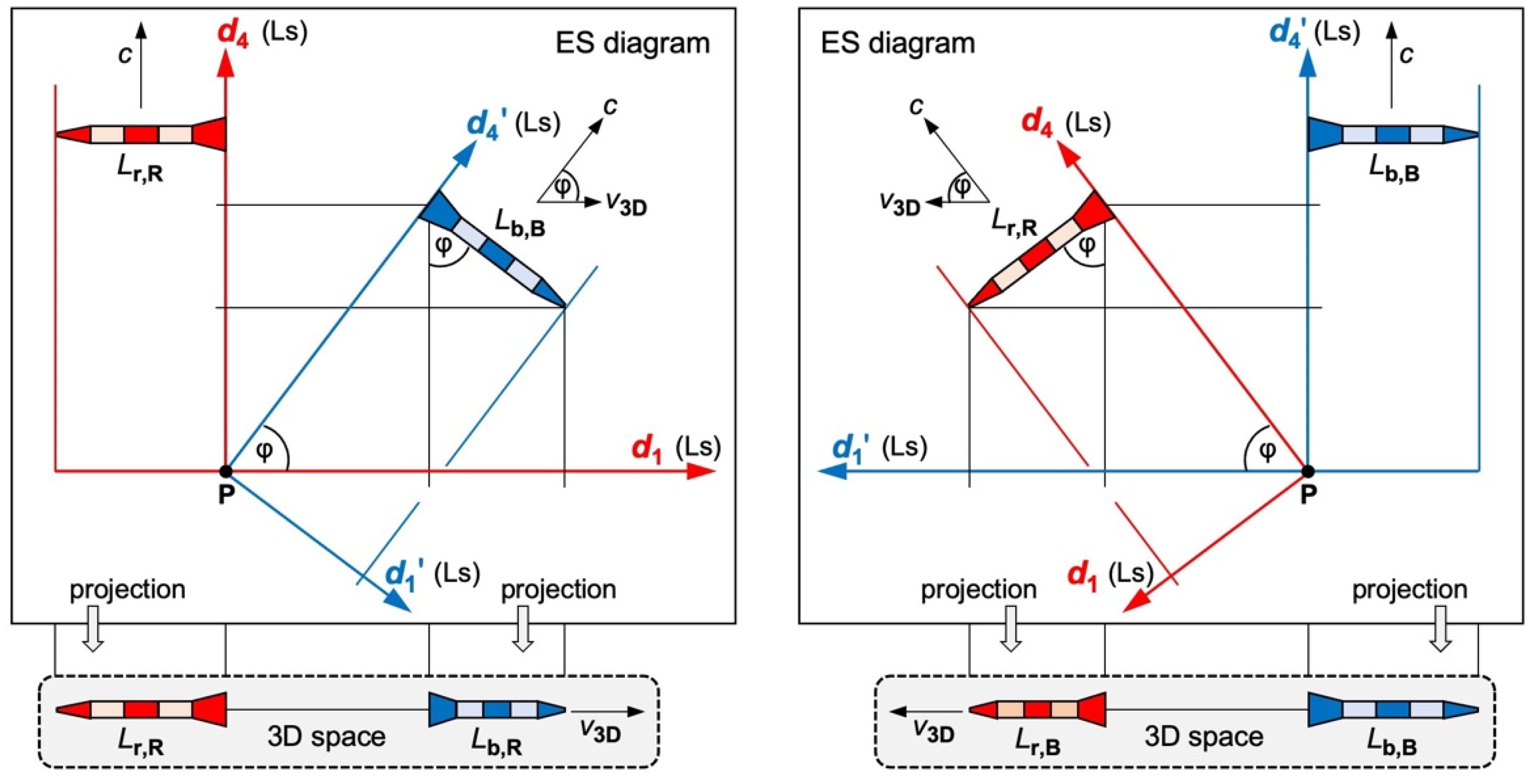
Figure 3.
ES diagram and 3D projection for two identical rockets. Top: In the ES diagram, the blue rocket accelerates in the axis . The red rocket moves in the steady axis . Bottom: Projection to the 3D space of R. The blue rocket accelerates against the red rocket. The red rocket is at rest.
Figure 3.
ES diagram and 3D projection for two identical rockets. Top: In the ES diagram, the blue rocket accelerates in the axis . The red rocket moves in the steady axis . Bottom: Projection to the 3D space of R. The blue rocket accelerates against the red rocket. The red rocket is at rest.
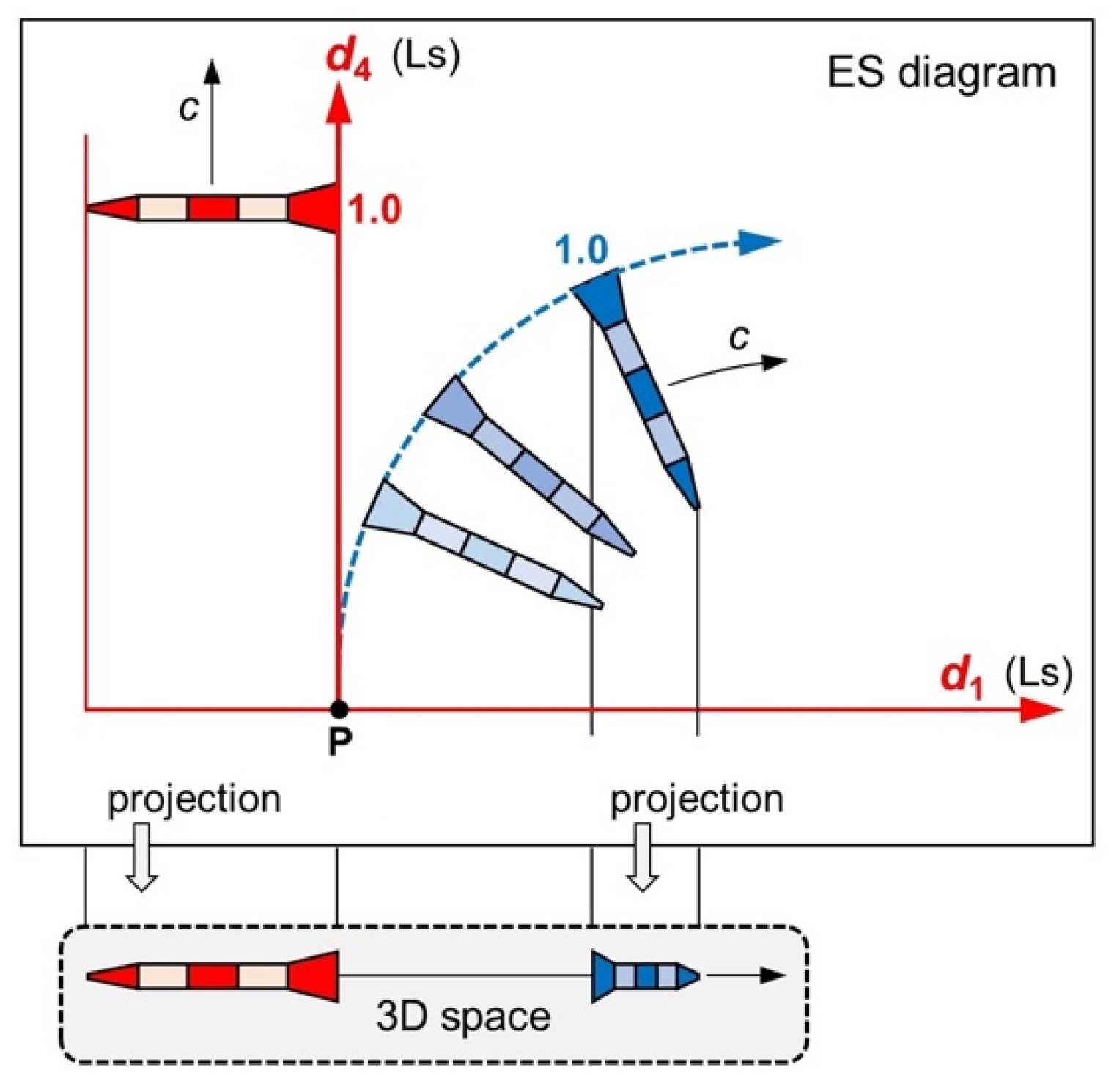
Figure 4.
Graphical solutions to three geometric paradoxes. Left: A rocket moves along a guide wire. In 3D space, the guide wire remains within the rocket. Center: An observer in a rocket’s tip tries to detect the reflection of a light pulse. Between two snapshots (0–1 or 1–2), rocket, mirror, and light pulse move 0.5 Ls in ES. In 3D space, the light pulse is reflected back to the observer. Right: Earth revolves around the sun. In 3D space, the sun remains in the orbital plane of Earth.
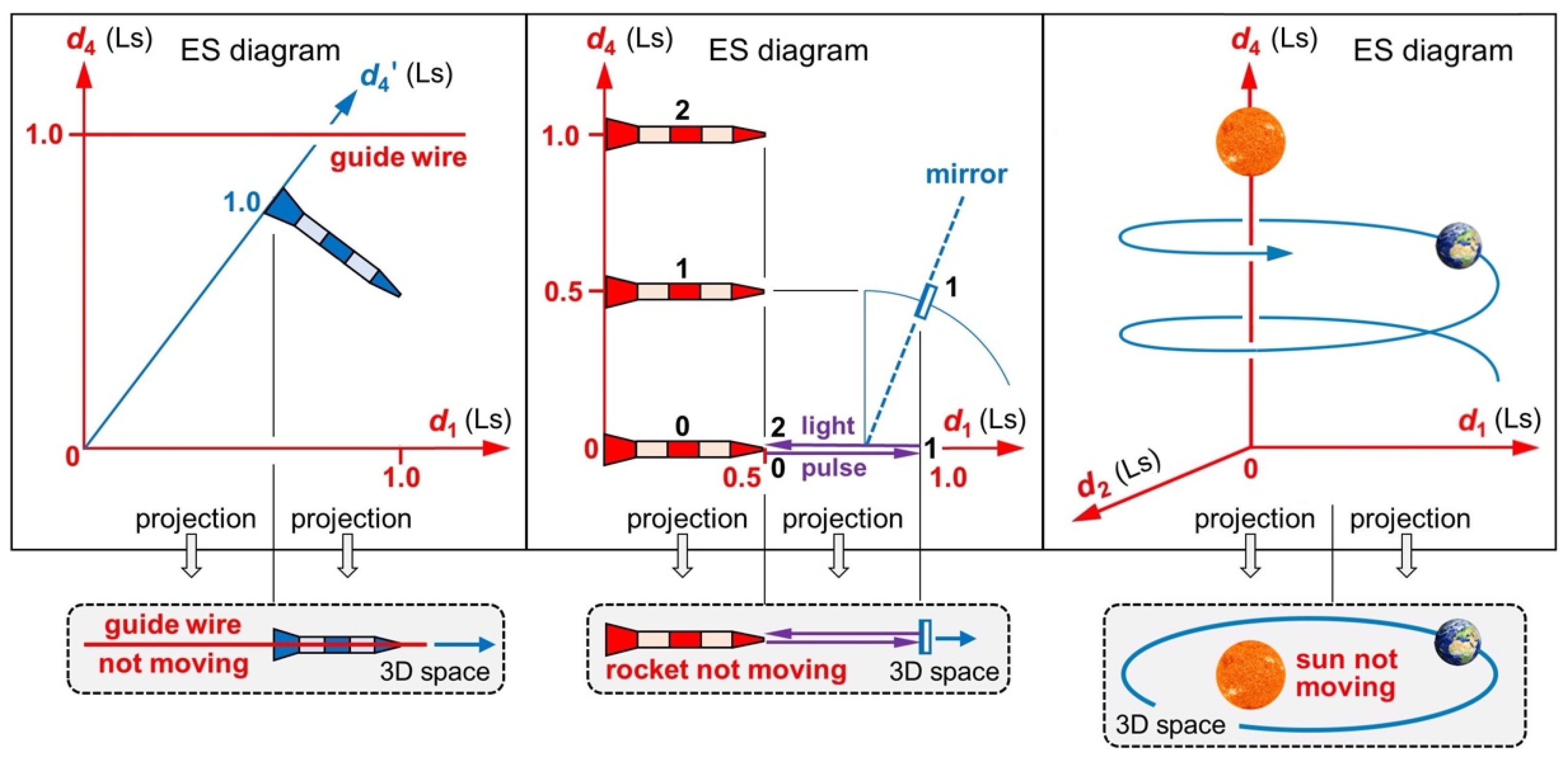
Figure 5.
ES diagrams and 3D projections (not to scale) for solving the mysteries 5.6, 5.7, and 5.10. The displayed circular arcs are part of a 3D hypersurface, which is expanding in ES at the speed . Left: The CMB is nearly isotropic because it was created equally in ( are not shown here). Right: A supernova S’ occurred when the radius was smaller than today’s radius . If a supernova S occurred today at the same distance , it would recede slower than S’.
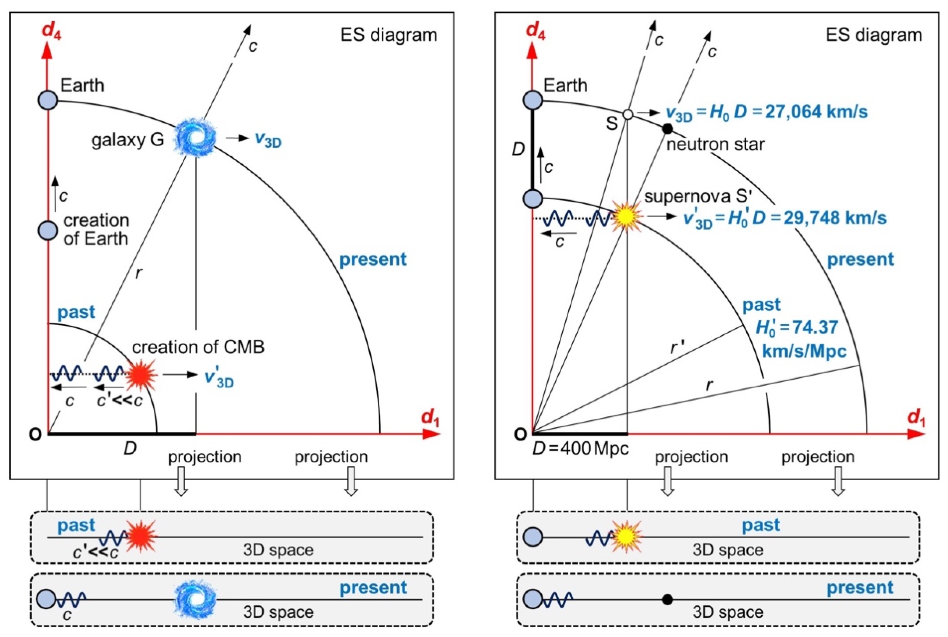
Figure 6.
Hubble diagram for 40 Type Ia supernovae. The horizontal axis displays adjusted speeds. All data including their uncertainties are listed in Supplemental Material [29].
Figure 6.
Hubble diagram for 40 Type Ia supernovae. The horizontal axis displays adjusted speeds. All data including their uncertainties are listed in Supplemental Material [29].
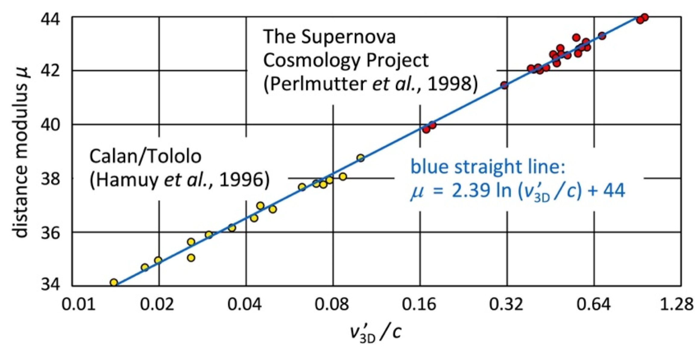
Figure 7.
Concept of wavematter. Artwork illustrating how an object can be deemed wave or matter. Wavematter comes in four orthogonal dimensions: propagation, electric field, magnetic field, and proper time. If I observe a wavematter (external view), I deem it wave or matter depending on its 3D speed. Each wavematter deems itself matter at rest (internal view or in-flight view).
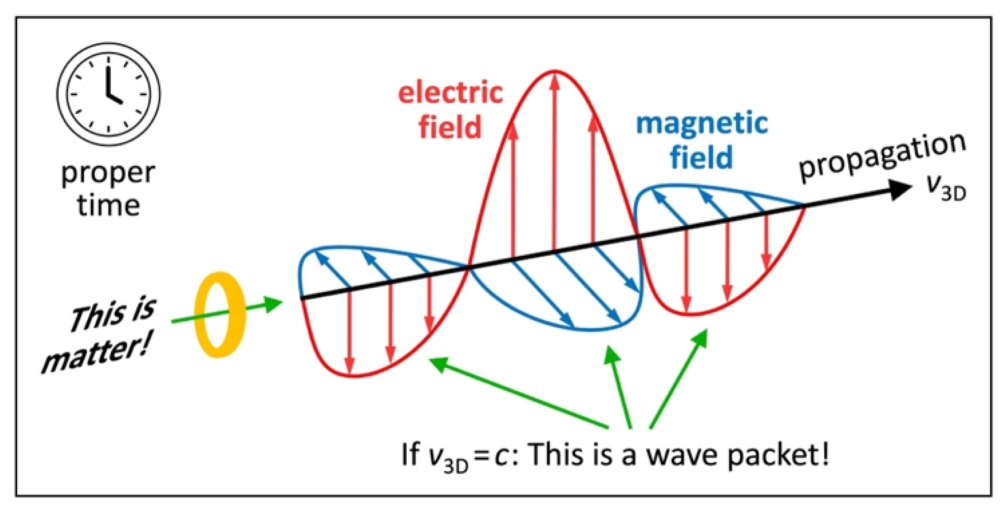
Figure 8.
ES diagrams and 3D projections for three wavematters. Top left: ES in coordinates where moves in . Top right: ES in coordinates where moves in . Bottom left: Projection to the 3D space of . deems itself matter at rest () and wave (). Bottom right: Projection to the 3D space of . deems itself matter at rest () and wave ().
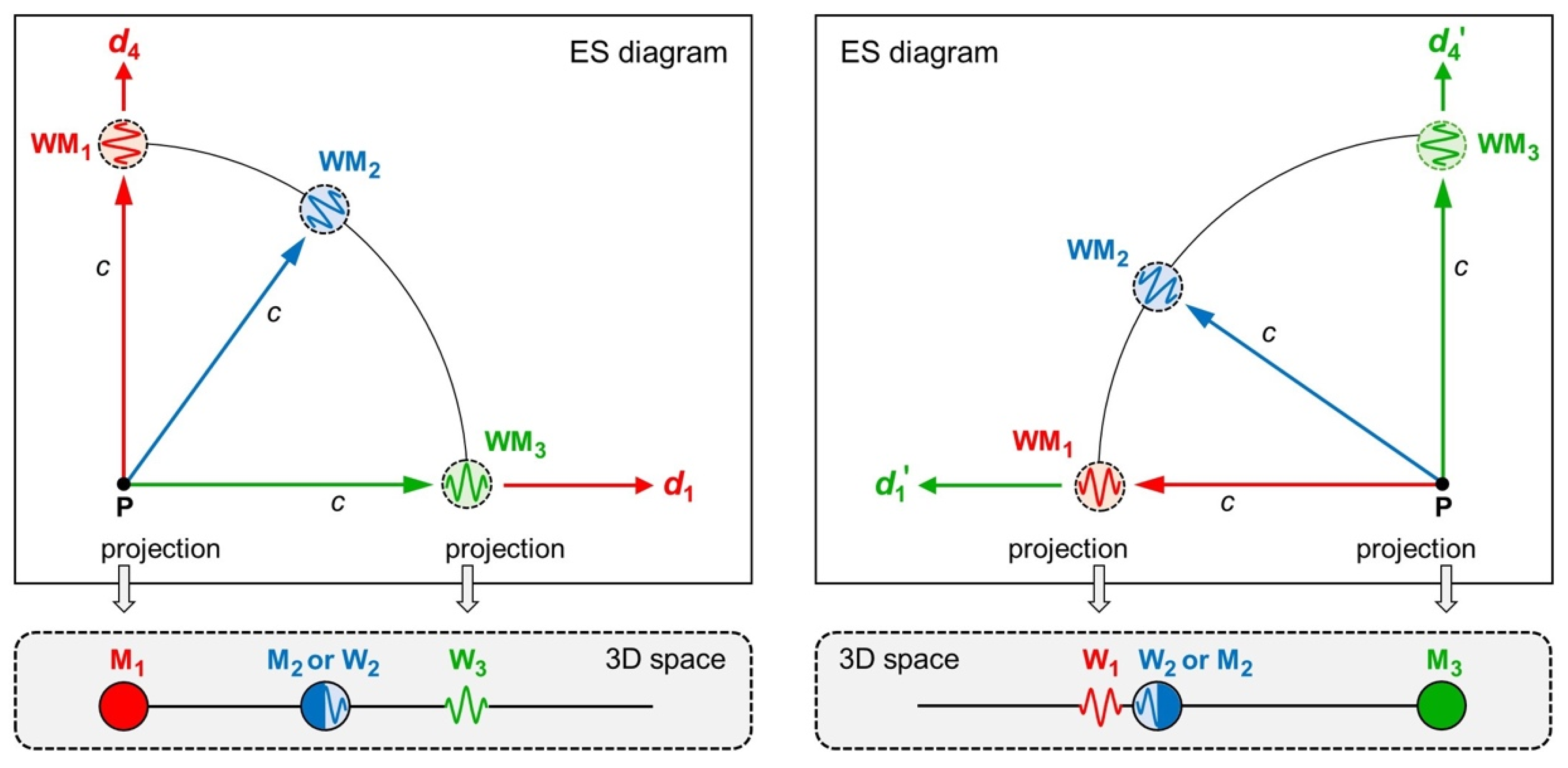
Figure 9.
Quantum entanglement in 4D ES. Artwork illustrating internal and external view. For each displayed wavematter, the axis disappears because of length contraction. It deems its twin and itself one object (internal view). For a third wavematter that moves in a direction other than , the axis doesn’t disappear. It deems the displayed wavematters two objects (external view).
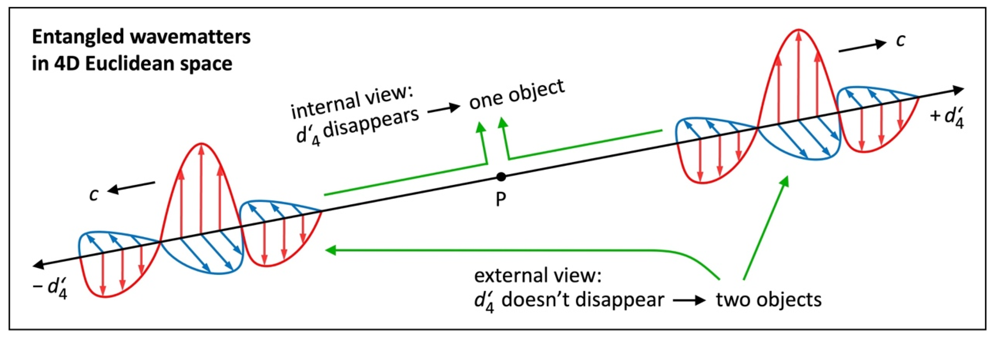

Table 1.
Comparing the Lambda-CDM model with the ER-based model of cosmology.
 |
Disclaimer/Publisher’s Note: The statements, opinions and data contained in all publications are solely those of the individual author(s) and contributor(s) and not of MDPI and/or the editor(s). MDPI and/or the editor(s) disclaim responsibility for any injury to people or property resulting from any ideas, methods, instructions or products referred to in the content. |
© 2023 by the authors. Licensee MDPI, Basel, Switzerland. This article is an open access article distributed under the terms and conditions of the Creative Commons Attribution (CC BY) license (http://creativecommons.org/licenses/by/4.0/).
Copyright: This open access article is published under a Creative Commons CC BY 4.0 license, which permit the free download, distribution, and reuse, provided that the author and preprint are cited in any reuse.


