
Submitted:
23 February 2024
Posted:
23 February 2024
You are already at the latest version
Abstract
One objective of this paper is to investigate bifurcation of solutions of Ornstein-Zernike equation in liquid state theory for the gas-liquid coexistence region of simple fluids. The analysis uses a discrete form of the Ornstein-Zernike equation in real space, together with a closure relation which provides nearly self consistent thermodynamic properties of fluids governed by interaction potentials like the Lennard-Jones potential. Accurate asymptotic forms of correlation functions are incorporated in the real space algorithm so as to mitigate the influence of cutoff length used in the discrete approximations. It is found that there is no spinodal on the vapor side on a sub-critical isotherm. But there are fold bifurcation points on the vapor and liquid sides together with a 'no-real-solution-region' in between. This is followed by a region of negative compressibility extending up to the spinodal on the liquid side. The emerging picture is quite similar to that in the case of the hypernetted-chain-closure. It is also found that complex solutions connect the physical solutions that exist outside the 'no-real-solution-region' as well as in region of negative compressibility. The second objective of the paper, in the light of bifurcation scenario, is to evolve an interpretation of the coupling-parameter expansion of correlation functions pertaining to the region of negative compressibility. It is shown that the expansion provides an accurate description of results of the restricted ensembles, implied in mean field theories and simulation methods. Bifurcation of singlet density to inhomogeneous distributions at a spinodal is also established using a simple equation, which uses the direct correlation function. Thus the paper reestablishes the fact that restriction to a homogeneous singlet density is the root cause of all inconsistencies found in the gas-liquid coexistence region.
Keywords:
Ornstein-Zernike equation
; bifurcation of solutions
; fold bifurcation points
; liquid-vapor phase transition
; coupling parameter expansion
; Lennard-Jones potential
1. Introduction
Ornstein-Zernike equation (OZE) and related developments form the main theoretical apparatus in liquid state physics; the other being computer simulation methods [1]. In addition to being an important branch of statistical mechanics, liquid state theory is an essential component in modeling the high-pressure equation of state [2], with applications in several branches of solid state science and high energy-density physics. So it is important to have quantitative knowledge about the physical and mathematical nature of solutions of OZE and the associated closure relations. Hence this topic has been the subject of detailed investigations over the last few decades. While the OZE equation is a relation defining the direct correlation function in terms of the total correlation functions , a closure relation relates them to the inter-particle potential . Common examples of closures include the Mean spherical approximation (MSA), Percus-Yevick (PY) closure and hypernetted chain (HNC) closure. There are also some approaches consisting of adjustable parameters to achieve self consistency, which provide same results via different routes to thermodynamics [3]. There exist also quite accurate, nearly self-consistent and explicit closures for specific potentials like hard sphere, the Lennard-Jones (LJ) potential, etc. [4,5].
A closure relation is solvable (in principle) so as to express in terms of explicitly, although this relation could be highly nonlinear. On using this relation, the OZE reduces to a nonlinear mapping of the form: for [6], and its solutions are simply the fixed-points of , which acts on functions defined in a suitable metric space. The specific details of the mapping will depend on the closure relation and inter-particle potential. Equally important, changes in fixed-point stability and bifurcation of solutions, resulting due to variation of parameters like density and temperature T occurring in , will also depend on the discrete approximations to , and the algorithm chosen to obtain solutions. For instance, algorithms may use 3D Fourier transforms for computing convolution integrals or simply employ real-space based methods. This is an important aspect to be considered when multiplicity and bifurcation of solutions to nonlinear eigenvalue problems are investigated [7].
As the correlation function decays for sufficiently large r, it is reasonable to assume that the constraint is satisfied in physically relevant situations. In fact, this integral constraint (IC) is a necessary condition for computing all thermodynamic quantifies and structure factor, as fluctuation theorem [1] relates it to reduced compressibility as . Further, violation of the IC in any part of phase-plane would generate problems in algorithms using 3D Fourier transforms, as the IC is necessary to ensure the existence of the transforms. This is important as many algorithms for solving OZE compute the convolution integral using Fourier transforms [8,9].
Baxter derived an alternate formulation of OZE [10], defined entirely in a finite range , where is a cutoff length introduced such that for . The vanishing property of is exactly valid within the PY closure when potential for . This formulation is derived by imposing the IC mentioned above, and is also useful even in cases where is negligible for where is chosen suitably. Approaches based on either Baxter’s formulation [11] or 3D Fourier transforms [12], have been used extensively to analyze bifurcation of solutions of OZE. In the latter case, a large cutoff length is introduced for use of discrete variables and FFT techniques. Violation of the IC may not be directly visible with any choice of , however large. So it is essential to introduce appropriate asymptotic expressions of correlation functions and their transforms, valid for , in the formulation [12]. Furthermore, this ‘OZE technique’ is unavoidable to obtain the correct variation of transforms in the Fourier variable k near its origin [12].
The OZE can also be written in the radial coordinate covering the full half-line , and solved recursively by applying Newton’s method [13]. The linear Fredholm integral equations (FIE) of second kind, which result within this approach, are readily solvable using a proper numerical scheme [14]. Of course, a discrete representation of variable r, sufficiently large cutoff length , and use of asymptotic expressions of functions beyond are needed in this approach (see §3). Note that numerical schemes for FIE are well developed, and there are also ways of reducing the half-line to finite intervals using appropriate transformations [15]. Adequacy of can be checked by generating a sequence of solutions (and integral quantities) for an increasing series of values of . The Converged solutions obtained with this approach need not satisfy the IC mentioned earlier. Analyses of solutions for the three closures, obtained with a finite element method (using piece wise linear functions) to solve the FIE in , together with asymptotic conditions for , have been done quite early [13]. Sensitivity of solutions to the chosen is also analyzed in this extensive work. There are differences in the results for some problems derived using this real-space method and Fourier transform method (see §2.1). This is plausible because the solutions obtained by the latter belong to a sub-space of the more general space of functions accounted within the former.
One of the objectives in the present paper is to investigate bifurcation of solutions of OZE combined with the Martynov-Sarkisov (MS) closure for LJ potential (see §2). This closure is chosen as it provides nearly self consistent results for hard sphere and LJ fluids [4]. A general real-space method, using piece wise quadratic functions for numerical integration, together with improved asymptotic conditions [16], in lieu of the simple ones used earlier [13], are employed in the present work (see §5). This mitigates the ill effects of chosen value of on the solutions obtained. The resulting real-space algorithms is first verified using an analytical solution [13]. Fold bifurcation points (turning points), on the vapor as well as liquid sides on any sub-critical isotherm, are first found using the pseudo arc length (PAL) continuation algorithm [17,18]. A ‘no-real-solution’ region, a non-physical branch of solution, regions of negative compressibility , and spinodal points are all obtained with the method. Further, bifurcation of solutions to the complex domain is analyzed [19], and the method is generalized to compute complex solutions in the gas-liquid coexistence region, wherever they exist (see §7.2).
In the light of the bifurcation scenario for OZE and MS closure, questions arise regarding the meaning of ‘solutions’ obtained via the coupling-parameter expansion (CPE) [20]. This approach uses expansion of correlation functions in terms of a parameter introduced in the potential, and provides real solution in the entire gas-liquid coexistence region [21]. The reference solution corresponds to purely repulsive part of the potential. Spinodal points, on vapor and liquid sides, with negative compressibility in between, are obtained on any sub-critical isotherm. The IC is violated in that region (see §2), thereby indicating some inconsistency in the CPE. However, the gas-liquid phase diagrams for Mie and LJ fluids, obtained via the compressibility route employing Maxwell’s constructions, agree with Monte Carlo simulation data very well. It also agrees excellently with results of an independent method (using thermodynamic conditions) based on free energy computed outside spinodal region [22]. It is important to emphasize that the second method does not use any data corresponding to the negative-compressibility-region. It is now shown (see §8.1) that data on isotherms through the spinodal region agree with those of transition-matrix Monte Carlo method [23]. Therefore, it is proposed (in this paper) that results of CPE are similar to those obtained via the restricted ensemble approach [13]. It is well known that the van der Waals equation, which yields negative compressibility region, is also derived from considerations of a restricted ensemble [24]. In addition, analysis of a simple equation for singlet density (see §8.2), involving the direct correlation function, shows that it bifurcates at spinodal points to an in-homogeneous distribution. This finding explains the origin of inconsistency arising out of negative compressibility obtained in any method.
Remainder of the paper is organized as follows. Basic equations and formulas used in the model are given in §2. Newton’s method in real and Fourier spaces, and some known results on bifurcation, are discussed in §3. Bifurcation of solutions (using real-space methods for MS closure ) inside the gas-liquid coexistence region are discussed in §4. Emergence of an infinite number of solutions in the spinodal region due to ‘singularity-induced bifurcation’ is bought out here. Discrete approximations of the FIE, arising in Newton’s method, using Nyström’s method are discussed in §5, while continuation algorithms form the topic of §6. Generalization of Newton’s method for complex solutions are covered in §7. The coupling parameter expansion and its relevance for restricted ensemble approach are given in §8. These sections (§6, §7, §8 ) also provide numerical results for LJ potential within MS closure. Finally, §9 summarizes the main conclusions of the present work.
2. Equations and formulas of the fluid model
The OZE introduces the short ranged direct correlation function via a convolution integral involving the total correlation function . For a one-component system of fluid particles, interacting via spherically symmetric potentials, it is written as
where is the average number density of particles. This equation needs to be supplemented with a closure relation involving , and the pair-potential . There is no exact analytical expression for the closure relation; however, all the basic closures are generally expressed concisely in terms of a ‘bridge function’ via the expression [1]
where , is Boltzmann’s constant and T absolute temperature. Further, denotes the indirect correlation function. So different approximate forms of generate different closures; for instance, the HNC closure is obtained with . The PY closure follows from , which yields . Note that PY relation also follows from HNC closure by using the linear approximation . The MSA closure is defined for potentials with a hard core, and it takes the form for (the hard core diameter) together with the hard core condition for .
A bridge function, which generates the Martynov-Sarkisov (MS) closure ( mentioned in §1) is given by [4]
The MS closure provides accurate thermodynamic properties for hard sphere as well as LJ potential [4]. The full LJ potential, which will be used throughout this paper, is given by
where and are energy and length parameters, respectively. Note that in Eq.(3) is a dimensionless number-density as is a length parameter. Further, in Eq.(3) is the pure attractive part of the potential as per the Weeks-Chandler-Andersen (WCA) prescription [25].
It is important to note that any solution of OZE must satisfy the relation , which follows by integrating it over the infinite space. Then, the integral condition (IC) , introduced in §1, turns out to be necessary to deduce an alternate relation for reduced inverse compressibility, viz. , where P is pressure. Therefore, the IC must be violated in regions in the phase-plane where . This is important because there can be situations where slowly decays to zero as , but I does not exist. Methods which assume that I exists (Baxter’s version of OZE or OZE in Fourier space) can not work reliably in such regions. So an algorithm using Fourier transforms, and a finite cutoff length , may give negative in some region, but those results have to be suspected [12].
Detailed analysis of the asymptotic variation of the correlation functions shows that varies for large r as [16]
where is the correlation length. This asymptotic form is valid for . The correlation length is also expressed as , , and the amplitude is positive. For the HNC closure, as easily derived from Eq.(2), varies as
so that it is a short ranged function compared to . For the MS closure (due to the bridge function), the asymptotic form for is found to be
which decays faster than that in the case of HNC closure. This feature has some consequences in determining the solution in the spinodal region. In the present paper, asymptotic forms either in Eqs.(5) and (7) or via Nyström’s interpolation formula (see §5) are used for the range .
When decays as for large r, it is necessary that for to exist. In these cases will decay as for HNC closure. This decay law do ensure the existence of the integral in Eq.(1), however, the IC will be violated for the range . Similar conclusion follows for MS closure in the range . While real-space methods would provide solutions in such cases, methods using Fourier transforms may face numerical problems.
2.1. Known results of bifurcation of solutions
Known results on bifurcation of solutions of OZE, on a sub-critical isotherm in the two-phase region, may be classified according to PY, HNC and MS closures. The following brief discussion uses and to denote densities at spinodal points on vapor and liquid sides, respectively. Similarly, and are used for the corresponding turning points (fold bifurcation points).
One clear result is from Baxter’s adhesive hard sphere model [26,27], which treats a system of sticky hard spheres within PY closure; the stickiness being modeled by an infinitely deep but vanishingly thin attractive square well. Analytical solutions of Baxter’s version of OZE (which assumes the IC mentioned in §1) show that does not exist. In fact, there is a for which , however, it lies on a solution-branch violating the IC. Then, the densities between and cover a ‘no-real-solution’ region. As density is increased further, another non-physical branch (violating the IC ) follows, which terminates at . The model has complex solutions within the ‘no-real-solution’ region.
Numerical treatment of Baxter’s OZE and PY closure, applied to a truncated LJ potential [11], yields both and and ‘no-real-solution’ in between. This work shows that, as in Baxter’s model, is finite at as well as . Methods using Fourier transforms and PY closure, also come to similar conclusions, either by incorporating proper asymptotic forms of correlation functions [12] or using large cutoff length [28]. Neither the former work (for hard-core Yukawa potential) nor the latter (for full LJ potential) report values. This could be because becomes negative in the range . The implicit assumptions involved in using Fourier transforms [12] show that this method should be restricted to regions where , where the IC is satisfied. Complex solutions have also been found for LJ potential near [28]. Solutions of OZE and PY closure in real space [13], also show similar results, i.e., evidence for and , but no . In addition, the last work also finds density regions (between and ) with negative compressibility.
For HNC closure, all approaches find and densities. Locus of these values (for different T), have been found using Fourier transforms and pseudo arc length (PAL) continuation algorithm [29]. Here it is also shown that values on the liquid side are very sensitive to cutoff length - a lower value of yields , but it is absent with . Importantly, the densities and are not obtained at all when proper asymptotic forms are incorporated into Fourier transforms[12]. Similar results together with complex solutions, near and , are also obtained using Fourier transforms [28]. But results of real space solutions [13] clearly show the occurrence of both pairs of densities and . In addition, regions of negative are also obtained [13] - however, is on non-physical branch and occur in the region of negative . Thus, for the HNC closure, there are some differences between these results and those obtained using Fourier transforms. In fact, results from real space methods are closer to those of Baxter’s model.
The occurrence of has been shown with several other closures, including the MS closure [30]. Thus it appears that a turning point on the vapor side of a sub-critical isotherm is found with all closures as well as methods. Emergence of complex solutions near , and occurrence of , have also been shown for MS closure using Fourier transform method. One of the aims in this paper is to investigate the complete bifurcation scenario within MS closure using real space methods.
Finally, note that analytical solutions exist to the hard-core Yukawa potential, within the MSA closure [31,32], which show the emergence of two real and two complex solutions in the entire range of and T in the super-critical region. Out of these, only one real solution approaches the ideal gas limit for small , and vanishes as the interaction strength . In the sub-critical region, there is a ’no-real-solution-region’ for a range of densities , because both solutions turn complex. Within this model, the spinodal lines, which now occur on both the gaseous and liquid branches, cover the ’no-real-solution-region’, and is always non-negative (as in Baxter’s model).
3. Newton’s method in real and Fourier spaces
As the indirect correlation function is more appropriate for numerical approximations, first Eq.(1) is rewritten in term of as
Newton’s method in real space applied to Eqs.(8) and (2), with bridge function specified in Eq.(3, is the approach used in this paper. Such an approach has been applied earlier, however, with PY and HNC closures, for a truncated and shifted form of the LJ potential [13]. Solutions to another well known non-linear equation in fluid physics, known as Born-Green-Yvon-Kirkwood (BGKY) equation, is also analyzed in this reference. This work used the asymptotic conditions for , with largest value . A finite element method, employing piece wise linear functions, was used to solve the equations in . A more general algorithm and several improvements, introduced in the present work, are discussed in this section.
Starting with an initial guess solution (for specified and T), and hence from Eqs.(2) and (3), improved approximations and are obtained using the first order correction term
where and is the derivative of with respect to y. The correction term obeys the linear equation
where is the error (or residual ) in Eq.(8) with the starting guess solutions and , viz.
Substituting from Eq.(9) gives the linear Fredholm integral equation (FIE)
where . First step in Newton’s method consists of solving this FIE, and obtaining an improved solution . The process is then repeated with new as the guess solution until certain convergence criterion is met. Usually, these iterations are terminated when a suitable norm (say, Euclidean) of is less than a prescribed value (say, ). This way of implementing Newton’s method is sufficiently general and is applicable with other closure relations; either is to be changed or an appropriate form of is to be substituted. For instance, in the case of HNC closure while for PY closure.
On writing , where is the cosine of the angle between and , the integral over in the interval [-1, 1] can be rewritten in r and . Then the terms in the kernel of Eq.(12) are given by
With these explicit definitions, the kernel of the FIE reduces to
Using same notations, the error term is given by
Now the FIE for is concisely expressed as
which can be solved using standard methods [14]. Quadrature formulas to approximate the integral for a specified value of r, and collocation rules form the tools in Nyström’s method to reduce a linear FIE to a matrix equation [15].
3.1. Version in Fourier space
If the integral constraint is valid, it is easy to rewrite Eq.(12) in Fourier space. On taking Fourier transforms it reduces to
Here k is the Fourier variable, and a ‘bar’ over the functions indicates their 3D Fourier transforms [22]. Note that first term on the right of Eq.(12) has appeared as in the denominators. The integral operator in this equation is defined in terms of Fourier transform. It is best solved using Krylov space-based methods like CGNR (Conjugate Gradient to Normal equations to minimize Residual) or GMRES (Generalized Minimum Residual), because the needed matrix-vector products in these methods can be computed via two Fourier transform operations [22]. To employ Fast Fourier Transform (FFT) techniques, first the radial coordinate is truncated to with a sufficiently large value of . It is also essential to use asymptotic forms of and , and their Fourier transforms, to develop a robust algorithm [12]. This method would develop numerical problems whenever the IC is violated as is the case close to spinodal points (if they exist), and on non-physical solution branches where compressibility is negative.
4. Bifurcation of solutions
Solving the linear FIE given in Eq.(17) and performing subsequent Newton’s iterations would provide a solution for one set of and T, if a suitable starting solution is provided. However, it is necessary to generate solutions for different values of on each isotherm, and on a number of isotherms. Bifurcation or branching of solutions occur at certain values of and T whenever new solutions appear. Bifurcation analysis, and continuation methods for tracing the different branches along , form a well developed topic. Excellent books cover all the mathematical and computational aspects of this fascinating field in nonlinear physics [17,18]. Applications of these methods for OZE and MS closure in real space are discussed in §6; the present section is devoted to a brief discussion of different branching scenarios.
Suppose is a solution of Eqs.(1) and (3) corresponding to density . Then, the change in the solution , due to a specified change in density, satisfies the linear equation
This equation follows exactly via the the same method elaborated in §3 for Newton’s method. For simplicity of notation, terms arising due to explicit dependence of on are omitted. Once again, , which corresponds to the solution at specified . Note that there is no term in the equation above, as occurring in Eq.(12), because satisfies Eqs.(1) and (3). The last equation may be written in operator form as
where is a linear operator and is the change in solution vector. Further, is the operator defining the OZE and a null vector. For a sufficiently small , solution of Eq.(20) will yield an approximate solution for the density . Then, starting with as initial guess, Newton’s method is applied to obtain a new solution-pair . In this way, a set of pairs is generated as points defining a solution-curve. However, in the neighborhoods and at values of where is singular (called critical points), this approach is bound to fail. In fact, the singularity of the linear operator signals bifurcation of solutions.
Analysis of bifurcation of solutions is usually done together with labeling the solution-curve using the arc length parameter ℓ. Thus, corresponds to the initial point where is known, and Eq.(20) is considered as a relation between and . For evolving the pair as functions of ℓ, Eq.(20) is modified as
Here and denote the components of the tangent vector to solution-curve at ℓ. The nature of the singularity of the operator , and the relationship of its null-space to , decide the type of bifurcation that occurs at that . These aspects will be covered in §6, using a discrete approximation to operator in Eq.(21). However, there is another type of bifurcation which is considered below.
4.1. Singularity induced bifurcation
The operator can be split into two parts, and Eq.(21) rewritten as
Here the part , for a specified density and corresponding , is defined as
and denotes the remaining part. Note that , which contains the function in its kernel, arises from the change in induced (via ) due to the change . If is non-singular, then Eq.(22) can be rewritten as , where the new vector is defined as Either or can be used for the solution-curve as far as is non-singular. However, at a value of where is singular, the matrix will diverge, and the associated changes in solution is termed as ‘singularity induced bifurcation’ [33]. But as is non-singular at , the vectors and hence are well defined, and these will vary smoothly across . So Newton’s method (via Eq.(12) or (17) ) will yield a solution to the original OZE in Eq.(8) at . Singularity induced bifurcation is associated with the divergence of the operator (or matrix) involved in one of the routes towards the solution.
Now, note that the operator involved in Eq.(1) or (8) - with the converged function - is the same as . Therefore, is also a solution at , where is an arbitrary constant and the eigenfunction corresponding to the zero-eigenvalue of . It is easily verified by direct substitution that the singularity occurs at whenever , where is the 3D Fourier transform of [22], and is the eigenfunction corresponding to zero-eigenvalue. A real value of k satisfying these conditions would exist when [12]. The pertinent point to note is that the solution violates the integral condition . Thus singularity induced bifurcations generate an infinite number of solutions (for differenr ), which violates the IC. These will occur for all values of for which ; such values do arise in the spinodal region on the isotherm (see Fig 2 ).
5. Discrete approximation to FIE
For developing discrete approximations, the integral over in Eq.(17) is truncated at cutoff length , and a quadrature scheme (like Trapezoidal or Simpson’s rule) is applied to approximate the integral for each value of r. Then a collocation method is used to generate a matrix equation that can be solved for at discrete set of quadrature points in . The kernel defined in Eq.(15) requires and in an extended interval when the solution is sought in . This requirement arises whenever the unknown function, in integral equations in 3D, depends only on the radial co-ordinate r. Therefore, suitable asymptotic forms for and are needed in . The ‘extreme’ asymptotic forms and in the last interval would necessitate the choice of a sufficiently large [13]. This problem, together with the efforts in computing the kernel and solving the FIE are, perhaps, the drawbacks of the real-space method. So the pioneering work [13] did not receive proper recognition.
A partial remedy to this problem, implemented in this paper, is to use accurate asymptotic forms and in . Using the current solutions and , Eq.(5) may be used to compute these asymptotic forms whenever . An alternate approach using Nyström’s interpolation formula, applicable to more general situations, is discussed at the end of this section. In developing a method for solving the FIE, first it is assumed that for . Note that and vanish (within tolerance) in the entire half-line when Newton’s iterations converge. Then, Eq.(17) is reduced to a finite interval as
After determining , and thereafter and , the asymptotic forms to be used in the next Newton’s iteration are updated. Thus, although there is lag by one iteration, the asymptotic forms in also converge if Newton’s iterations converge. The real-space method implemented in this paper, with an accurate method to solve the FIE in a finite interval [14,15], would provide solutions even when the IC is violated (see §2).
The Nyström’s method is commonly employed to transform a FIE to a matrix problem [14,15]. In the procedure adapted here, the upper limit is chosen such that , where . Thus, there are a total of major intervals and solution-points in the discrete problem. The unknowns , where for , are the dependent variables. It is assumed that is even and the integral in Eq.(24), for any value of r, can be approximated using piece wise quadratic polynomials. In the interval (j even), any function is expressed as
Then, introducing certain weight factors (which depends on r as explained below) to account for the volume element , Eq.(24) is approximated as
For writing this equation, it is assumed that is a quadratic polynomial in in , as defined in Eq.(25). The collocation rule in Nyström’s method amounts to enforcing this equation at the discrete set of values , which reduces it to a matrix equation
where and are dimensional vectors with components and . Elements of the dimensional matrix are defined as
where denotes Kronecker delta. Two types of weight factors have been introduced here for reasons explained below. Note that the first row of (for which ) is denoted as for . The first column of is just the transpose of its first row. The remaining elements are denoted as for . Components of the source (residual) vector are given by
Note that all the components would approach zero, if Newton’s method converges.
As the integrals , and similarly for , the two types of weight factors, , introduced above are
These definitions account for the volume element in the integral operator exactly, and allow to retain explicitly as an unknown in the discrete equations. Further, for evaluating the integrals and , additional weight factors are introduced as
Note that and , where the proportionality factors are universal real numbers. Furthermore, the recursion relations defined as
for , allow the integrals and to be expressed as
Here, i and j vary over . Then the discrete approximation to the kernel reduces to
This method for computing the matrix elements, which relies on recursively defined one-dimensional arrays, is much faster in comparison to direct evaluation.
In Nyström’s method, Eq.(26) (known as Nyström’s interpolation formula) is useful to determine , and thereafter , for arbitrary values of r in the half-line [14]. In this paper, the interpolation formula is employed for the set , to update the asymptotic forms as and . This way of updating the asymptotic forms would work as far as Newton’s method provides a solution to Eq.(1), even in situations where the integral condition is violated.
5.1. Checking the algorithm
To check the accuracy of the discrete algorithm, consider the nonlinear integral equation [13]
It is easily verified, by direct substitution, that it has the exact solution when the function and n are chosen as and . Alternatively, the second integral term can be written as (see Eq.(13 also), and the solution verified using Fourier transforms. This non-linear equation is similar to the OZE [13], and may be used to evaluate the dependence of numerical error on mesh size in discrete approximation. Application of Newton’s method, that follows exactly the same steps leading to Eq.(24), yields the linear equation
where the kernel and source terms are given by
Here is a guess solution. Its asymptotic form needed in the interval , for computing the integrals in these equations, is taken as the exact solution. The matrix equation obtained in the discrete version of Eq.(36) is expressed as
where the matrix elements and source vector can be computed as done earlier. In fact the matrix elements are defined as in Eqs.(28) with replaced by . The latter is to be computed as done in the case of Eq.(34). New arrays as defined in Eq.(32) have to be generated in advance to obtain . Similarly, the components of source vector are defined as in Eq.(29). Due to the use of exact asymptotic form of , the error in the discrete approximation arises from the use of quadratic functions only.
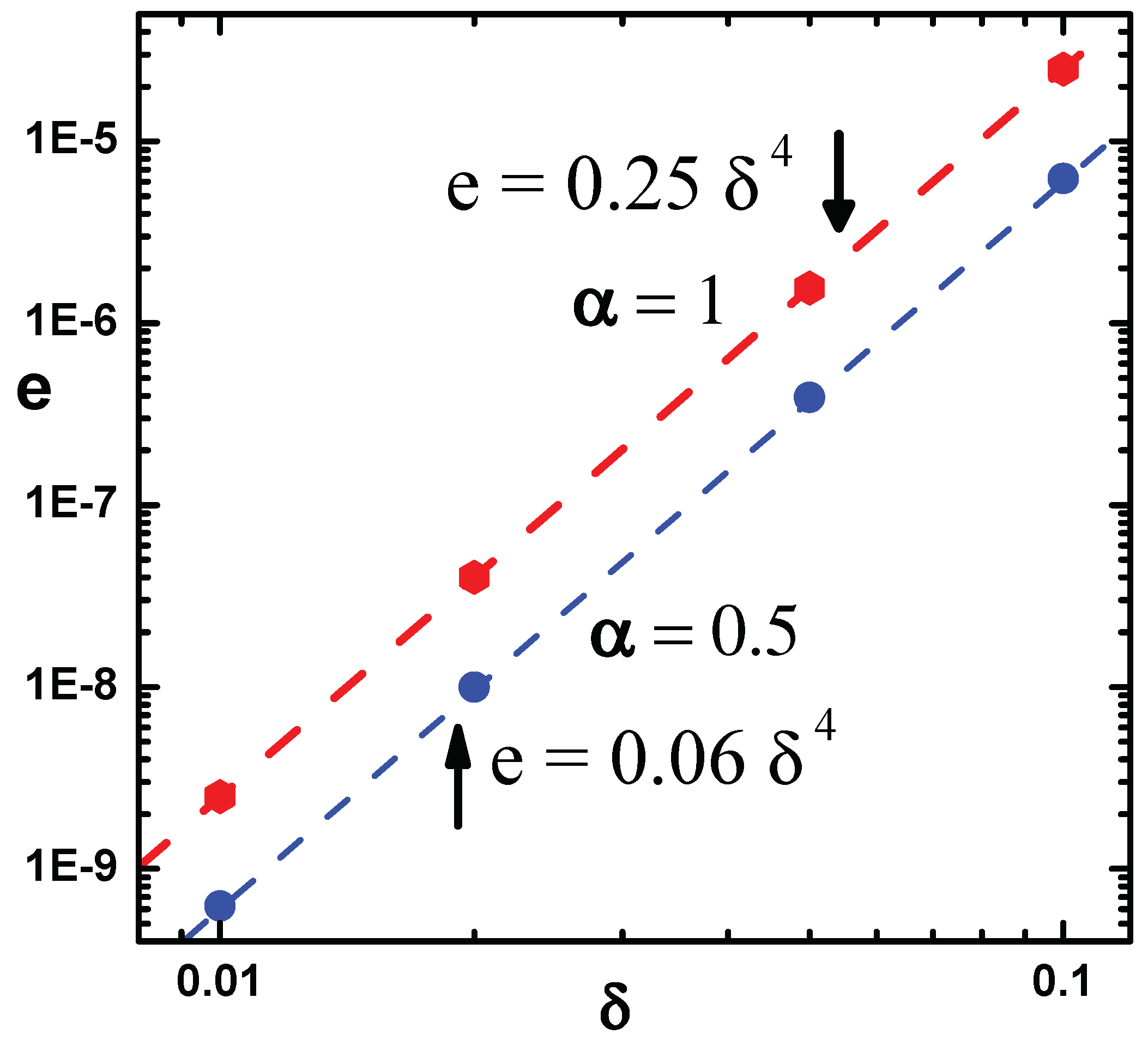
Results of computations (with cutoff length ) for the error (infinity-norm) versus mesh size are plotted (symbols) in Figure 1 for and . The broken lines are fits given by and for the two values of . As expected, the global error reduction factor of Simpson’s rule is realized in the algorithm.
Figure 1.
Euclidean norm of error e in versus mesh size are shown (symbols) for and . Broken lines are fits given by and for the two cases.
Figure 1.
Euclidean norm of error e in versus mesh size are shown (symbols) for and . Broken lines are fits given by and for the two cases.
6. Continuation algorithms
The discrete set of equations and Newton’s method would provide a solution for given and T, if a suitable starting solution is provided. More appropriately, solutions on an isotherm, starting from to an upper limit are derived using the pseudo-arc length (PAL) continuation algorithm. This generates a sequence of solutions , , and hence a solution-curve, within the discrete approximation. The PAL algorithm, employing Fourier transforms to compute convolution integrals is already used to generate the ‘no-real-solution’ boundary lines for LJ and hard core Yukawa (HCY) potentials within the HNC closure [29]. This method is likely to fail on or inside the spinodal region on a sub-critical isotherm because the Fourier transforms of functions do not exist.
This section is devoted to discussing these methods for OZE and the MS closure (Eqs.(1) and (3)) in real-space. The discrete version of Eq.(20) is expressed as
where is a dimensional null vector. The elements of are given by (see also Eq.(29))
In the limit , Eq.(40) implies a system of ordinary differential equations of the form . Then, Euler’s forward difference scheme implied in Eq.(40), or more accurate difference schemes are used to solve the differential equations, with an appropriate initial condition at . For a sufficiently small , solution of Eq.(40) will yield an approximation for the density . Thereafter, starting with as initial guess, Newton’s method is applied to obtain a new solution-pair . In this way, a set of pairs is generated as points defining the solution-curve. Generating a discrete set of solutions via Eq.(40), and subsequent Newton’s method, is called the first order continuation method. Incidentally, zeroth order continuation amounts to repeated use of Newton’s method with solution from previous value of as the initial guess. First order continuation belongs to the class of ‘predictor-corrector’ methods: solution to Eq.(40) provides the predictor while Newton’s method works as a corrector.
6.1. PAL algorithm
In the neighborhoods and at values of where is singular (called critical points), first order (or zeroth order) method will fail and different continuation algorithms are needed. In these algorithms, the pairs are considered as points on a curve in dimensional space, which is labeled by the arc length ℓ (see §4). Thus, corresponds to the known initial point . Assuming that solution-pairs up to are already obtained, Eq.(40) is modified as (see Eq.(21))
Here and denote the components of the tangent vector to solution-curve at . However, now there are unknowns in Eq.(42), but the deficiency is removed by normalizing the tangent vector to unit length as , where denotes the Euclidean norm of . A simple way to impose this normalization is to append Eq.(42) with an additional equation, , which assigns value unity to the component of . Thus Eq.(42) is modified as
where is a unit vector with component unity, and superscript t denotes transpose of the column vector. The value of is finally recomputed by imposing the normalization condition of the tangent vector. The choice of k is somewhat arbitrary; one choice would be such that is largest of all components. This method will not fail even at a fold bifurcation point, as the enlarged matrix in Eq.(43) is non-singular (see §6.2).
To obtain a proper predictor in PAL algorithm, the arc length equation defined as is added to Eq.(40) to close the system of equations. Here is the Euclidean norm of . Being nonlinear, this relation is not useful directly. So a linear version of the same (hence the name pseudo arc length), expressed as , is used in PAL algorithm. This relation follows by replacing and with the corresponding derivatives, which is well justified if is sufficiently small. Using their latest values computed via Eq.(43), the system of equations to be solved in PAL algorithm, for predicting the solution from , is
This solution readily provides the predictor to next solution pair as and . Newton’s method is applied as a corrector, starting with and , to this extended system of equation. The corrector iterations are performed by solving the equation
Note that is now present in the source vector as the predicted (as well as subsequent) solutions do not lie on the solution-curve. All the matrix elements in , tangent components and residual vector in Eq.(45) are to be updated, as iterations progress, using the most recent solutions and at arc length . In a more commonly used version of the PAL algorithm, an additional condition that the correction vector is orthogonal to the tangent vector is employed. Correction iterations converge faster as these proceed in orthogonal direction to the tangent vector. This makes in the source vector and Newton’s corrector equation reduces to
6.2. PAL algorithm and singularities
PAL algorithm outlined above will work in situations when is singular for a particular , but has a simple rank deficiency. Thus its rank is at the singularity, i.e., one less than the dimension . In that case its zero-eigenvalue is simple, which means that the null space is one-dimensional. Now, the rank of the augmented matrix can be either or . In the first case, is called a fold bifurcation point, where as in the second case it denotes a simple bifurcation point corresponding to either trans-critical or pitchfork bifurcations [18]. For the case of fold bifurcation point (case-1), as the rank of augmented matrix is , there is only one vector that satisfy the equation
which is same as the tangent equation. Now, the augmented matrices in Eq.(43) or (44) can not have a zero-eigenvalue, as the same vector can not also satisfy the eigen-value equation. In this case the PAL algorithm allows one to move on the solution-curve smoothly. Determinant of will change sign at the fold bifurcation point, and can be monitored to locate the same [18]. In fact, zeros of linear interpolation polynomials of solutions, constructed with successive positive and negative values of determinant, provide good approximations to the fold bifurcation point [18]. The singularity of at the fold bifurcation point, say at , implies a consistency condition (for a non-trivial to exist) that has to be orthogonal to its right eigenvector - same as the eigenvector of . However, as the rank of the augmented matrix is , the vector can not be expressed as a linear combination of the columns of , i.e., there does not exit a non-trivial vector defined as . So the consistency condition is satisfied only when the slope . Using Taylor’s expansion, it is shown that a negative value of second derivative , with respect to ℓ, leads to a fold turning to left at , while a positive value yields a right-turning fold (see Figure 2).
Because the rank of augmented matrix (which has columns ) is for the case of simple bifurcations (case-2), there are two independent vectors , for , that satisfy the equation . In fact, these two tangent vectors can be determined [17,18], thereby making it possible to trace both branches passing through the bifurcation point. Applications of these ideas are discussed below (see §7.2, §8.2).
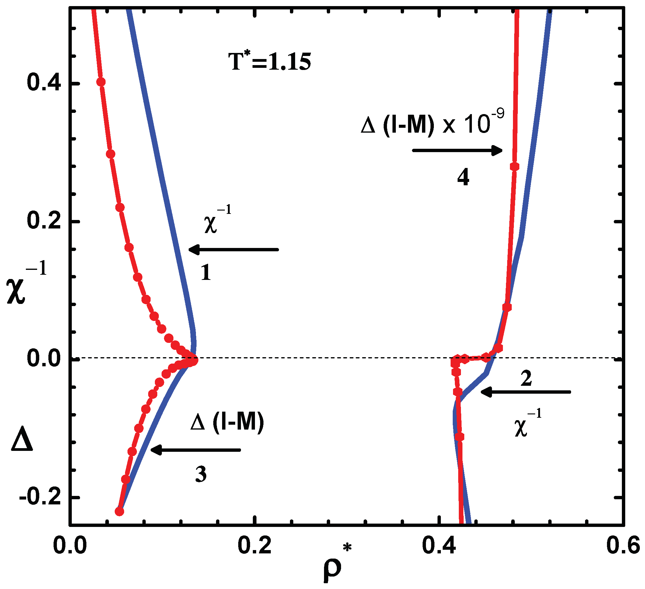
The methods described above is now applied to LJ potential with MS closure. Results obtained for the isotherm corresponding to reduced temperature are shown in Figure 2. Mesh size and cutoff length leading to are used in the discrete approximations. Proper asymptotic forms for and , as explained in §5, also are employed. Inverse compressibility and determinant of the Jacobian matrix are plotted versus reduced density . This isotherm is well in the sub-critical region as the critical temperature is . Fold bifurcation points, corresponding to , occur at and on the vapor and liquid sides, respectively. Similarly, spinodal points at which , are found at and , on the two sides. The difference between the two types of densities is very small on the vapor side, although the fold bifurcation point is larger than the spinodal point. The solution-branch for is nonphysical because increases with density. So it may be concluded that the spinodal at is not on a physical branch. The fold bifurcation and spinodal are well separated on the liquid side, and between them. While there is a unique solution branch for densities higher than the spinodal (on the liquid side), two branches are found for densities lower than the same on vapor side. These results are quite similar to those found via real-space approach for HNC closure [13]. However, computations employing Fourier transforms did not find density-regions where is negative [28]. Similar results are found for other isotherms corresponding to and .
Figure 2.
Inverse compressibility versus along isotherm for , in the vapor side ( curve 1) and liquid side (curve 2) for LJ potential. Determinant of the Jacobian matrix on vapor and liquid sides are shown in curves 3 and 4, respectively. While vanish at and , fold bifurcation points (where determinant vanish) are at and (see text in §6.2).
7. Generalization for complex solutions
Complex solutions to OZE and PY closure, inside the two-phase region, were originally found for hard spheres with stickiness [26], and LJ potential [11]. While these investigations employed Baxter’s version of OZE, similar results were also found by generalizing the Fourier transform method to the complex domain [34]. More recently, complex solutions are found for LJ potential with HNC [35] as well as several other closures [28]. All these results may be thought of as bifurcation from real to complex branches of solutions [19]. Most interestingly, bifurcation analysis to complex domain connects different branches of real solutions, which appear as disconnected branches if restricted to real valued functions [19]. In this section, the real-space method to OZE and MS closure is generalized to the complex domain.
If and are generalized as and , where the subscripts R and I denote the real and imaginary parts, respectively, then Eq.(8) will yield separate equations for the real and imaginary components. Alternatively, the linear Fredholm integral equation in Eq.(24), can be generalized as
where the kernels and are given by
For simplifying equations, is introduced, where, and (subscript Z denotes either R or I) are redefinition of Eqs.(13) and (14) employing and . Therefore, they can be computed as in the case of real solutions. Similarly, provides the real and imaginary components, where it is assumed that the bridge function is defined with the real part . Asymptotic forms of these functions in are needed in computing the kernels given above. Residual terms and are found to be
where . Discrete form of Eq.(48) is obtained following the same procedures and formulas used for the case of real solutions. There are no additional complications, although the dimension of the matrix equation to be solved is doubled to . Nevertheless, some of the formulas are listed in next section for completeness.
7.1. Discrete form for complex solutions
For complex solutions, it is straightforward to generalize Nyström’s interpolation formulas in Eq.(26) as
Application of the collocation rule readily yields the matrix equation
Elements of the matrices are defined exactly as in Eq.( 28) with (where Z denotes either R or I) in place of . Computation of matrix elements also proceeds exactly as in the case of real solutions, however, additional arrays, like in and ( see Eq.( 32) ), need to be generated with real and imaginary components and . The known vectors and are also computed using expressions analogous to those in Eq.(29).
Nyström’s interpolation formulas in Eq.(51) are useful to determine , for arbitrary values of r along the half-line , as in the case of real solutions. Thereafter are readily computed using . These are employed for the set of ordinates in the range to update the asymptotic forms to and . Continuation of solutions for different values of is obtained using the same PAL algorithm, generalizing Eq.(43) to get tangent vector, Eq.(44) for predictor and Eq.(46) for corrector iterations. Of course, the starting point is and it is necessary to employ dimensional matrices throughout.
7.2. Complex bifurcation
The method outlined above, is along the well known procedure to look for complex solutions to non-linear equations [19]. The imaginary components of the solutions are automatically generated, as discussed below, on continuing the solution along the arc length - it is found unnecessary to tweak the OZE by adding an imaginary term as done in earlier works [28,35]. For the complex solution, the tangent equation in Eq.(47) still applies, but the matrix , and vectors and are taken as complex objects (with subscripts R and I denoting real and imaginary parts, respectively). This equation together with its derivative with respect to ℓ, are written as
Here , and denote derivatives with components of and , respectively. Note that is a complex matrix of dimension and , which denotes a direct product, is a dimensional vector. Expressions for these are easily derived using Eqs.(28) and (41), after generalizing them to complex solutions. As explained earlier (with reference to Eq.(19), the explicit dependence of , and hence of , on is omitted, which explains the absence of the term. Also, and are second derivatives with arc length ℓ. At the fold bifurcation point , the identities and hold, although and can still be complex vectors. So at density , Eq.(53) reduces to
Now, Eq.(54) shows that where is the (real) eigenvector corresponding to zero-eigenvalue of and an arbitrary (complex) constant. The corresponding eigenvector of is denoted by . On substituting for , and pre-multiplying with , Eq.(55) yields
This equation consists of two unknowns, however the possibility of choosing multiple values of (consistent with the equation) would indicate the emergence of different solution-branches at . Now, has to be either purely real or purely imaginary . The former case yields , where and . This provides the real-branch at found earlier in §6.2. The latter case gives , which shows the emergence of imaginary branch at .
Exactly similar analysis is done for the spinodal point starting with the discrete version of the tangent equation in Eq.(22). Its complex version and derivative with ℓ are expressible exactly as in Eq.(53), although with minor differences. Now, denotes the discrete version of operator , and also contains an additional term arising out of the operator in Eq.(22). Again, all the matrices and vectors (except ) are real at the spinodal density , however, . Thus, the equations to be analyzed at are given by
Note the presence of extra terms, in comparison to those in Eqs.(54) and (55), because . Now, the crucial point is that , because the solution exists, although is singular at . Then, the general solution of Eq.(57) is expressed as , where is a (complex) constant and is a particular solution. This solution is chosen such that , as any component of along is absorbed in . Now, the steps leading to Eq.(56) are repeated to obtain the quadratic equation: . Here A is already defined, and . The remaining constants are obtained by replacing f by v in A and , respectively. That is, and . The quadratic equation in has two real roots or a pair of complex conjugate roots, depending on the values of and other parameters. In addition, it yields . The two real values of give on the real solution-branches while the complex conjugate pair generates the complex solution-branches.
Thus, two sets of complex solutions may occur in the two-phase region; one originating at the fold bifurcation point and the other at the spinodal point. The second may be absent in some specific cases, as in the case of Baxter’s model [26].
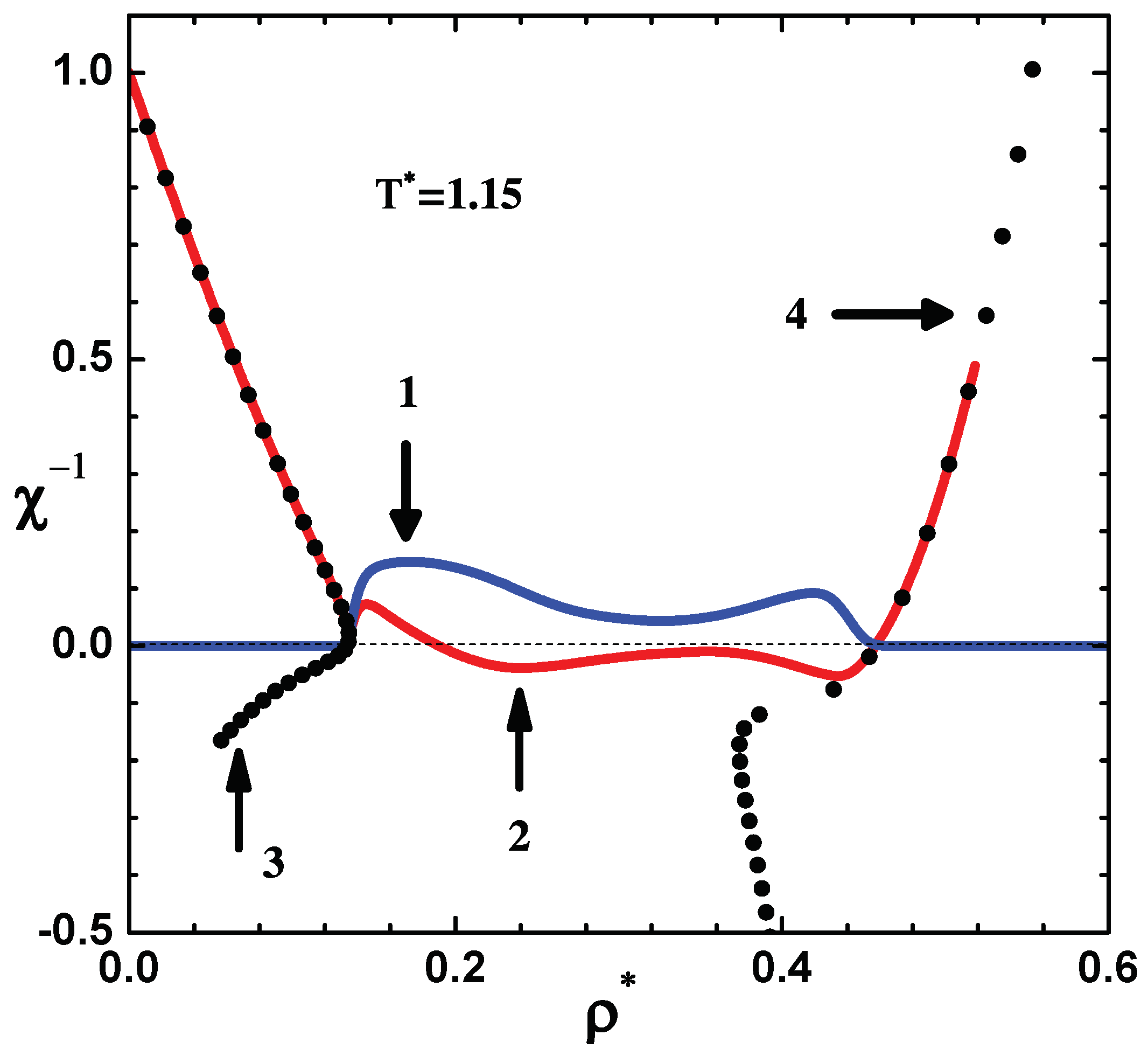
The algorithm described above is applied to LJ potential. Mesh size and cutoff length , which yields , are used. Asymptotic forms for real and imaginary parts of and are also used, as explained earlier in §7.1. Computations started at and the complex solutions are generated automatically by the algorithm. Complex solutions and lead to complex values for thermodynamic quantities. Values of inverse compressibility against , along isotherm for , are shown in Figure 3. Imaginary part (red curve1) is identically zero outside the spinodal region, while the real part (blue curve 2 ) connects the spinodal points on vapor and liquid sides. Symbols, marked as 3 and 4 in the figure, show versus from purely real solution branches discussed in Figure 2. Importantly, the complex solutions are seen to cover the entire spinodal region, as clearly evident on the liquid side. It is possible that there is another complex branch connecting the fold bifurcation points, however, this was not found in the results. Special procedures to trace a complex branch at the fold on liquid side may be necessary for this. Comparison of (on real branches) in these figures also shows that all its variations are retained either with or .
Figure 3.
Complex inverse compressibility versus along isotherm for . Real part ( red curve2) and imaginary part (blue curve1) connect spinodal points on vapor and liquid sides. Symbols (marked as 3 and 4 ) show vs from purely real solution branches (see Figure 2). Note that the complex solutions cover the entire spinodal region (see text in §7.2).
8. Coupling parameter expansion
The coupling parameter expansion (CPE) starts with splitting the potential as , where and are, respectively, purely repulsive and attractive components, as per WCA prescription [25]. The coupling parameter tunes the strength of the attractive potential; corresponds to the reference part while provides the full potential. Now, all correlation functions also are considered as functions of . In CPE, these functions are assumed to be analytic around , and expanded as Taylor’s series in about the respective functions corresponding to their reference parts [21]. Thus, the function is expanded as
Here denotes the derivative () of at ; being the total correlation function for reference potential. Other correlation functions, and , are also represented via such series expansions. The main assumption in CPE is that these expansions converge over the entire range , and the contributions from the attractive part of potential are adequately accounted via the derivatives like . Truncation of the series at zeroth order yields the first order perturbation theory [1]. But the general formulation of CPE can incorporate quite higher order derivatives, however, by taking recourse to the OZE [22].
Using the binomial expansion of derivatives of product of two functions, the derive of Eq.(8) is readily found to be
where {} are the binomial coefficients. Similarly, the closure relation in Eq.(2) is differentiated n times to obtain
where is derivative of computed at (see Eq.(9)). The derivative of bridge function, with respect to , are expressed as , so that contains only derivatives of of order less than n. The derivatives for the MS closure are obtained via recursion relations [21,22]
The summation term contributes only for ; so this recursion equation provides explicitly at all orders. Now, substitution of the above expression for in Eq.(60) gives the linear equation
where . Note that the kernel of the above FIE is similar to that in Eq.(12), and so can be re-expressed as in Eq.( 15). Computation of correlation functions and for the reference system (on any isotherm) is readily done using Newton’s method and first order continuation. No singularities are encountered for the reference system as it is purely repulsive. The FIE is easily converted into a matrix equation like using Nyström’s method elaborated in §5. The source vector contains only derivatives of order less than n, and the matrix to be inverted is same at all orders.
The derivatives and are short ranged functions, just like and , and so their Fourier transforms exist even in the coexistence region. Therefore, it is not necessary to continue in real-space; the convolution integrals in Eq.( 63) are easily computed in Fourier space. Taking Fourier transforms yields
This equation is identical to that obtained earlier [21,22]. Further, it is quite similar to Eq.(18), which represents Newton’s method in Fourier space. However, the factor in the denominators will never become zero as it refers to the reference system. The operator involved in Eq.(64) is the Fourier transform integral, and so this equation is easily solved via Krylov space methods [21]. For applications, is set to 1 in Eq.(59), and the series is terminated at a suitable order. All results obtained below use 7th order expansion [22], thus keeps terms up to .
Two independent methods for computing thermodynamic quantities, one via the free energy route and the other using the compressibility route, were used to obtain the phase diagram of LJ fluid [22]. Both approaches agree very well each other, and with results derived from simulation data [36]. The former method does not need data in the spinodal region for computing the phase diagram; it imposes equality of pressure and chemical potential of the gaseous and liquid phases. But the latter uses integration of inverse compressibility along , starting from . Because it is computed as , negative values of - signaling slow decay of - are obtained along any isotherm in the sub-critical region, which is discussed next.
8.1. Negative compressibility
Convergence of the CPE was analyzed in detail earlier [22]. There it is shown that the series truncated at 7th order, which retain terms up to , converge to well defined functions in the super-critical as well as sub-critical regions for LJ fluid. However, the integral constraint is violated in regions where is negative (see §2). Suppose and are solutions (presumably converged) obtained via the CPE. Then, the starting Eq.(8) shows that is also a solution where satisfies the homogeneous equation , and an arbitrary constant. In fact, is the eigenvector corresponding to zero-eigenvalue of the integral operator in OZE, with a given function . It was argued in §4 that such functions do exist whenever is negative. Equally important, the spatial integrals of and do not exist. Thus CPE gives rise to an infinite number of solutions, which violate the integral constraint in the spinodal region.
It has been argued [13] that Monte Carlo simulations [37] and mean field theories of fluids [24] can be constructed within a restricted ensemble approach. Here the total volume occupied by the system is divided into a large number of cells, and the particles in each cell is restricted to move within that cell. This restricts the range of allowed statistical (number) fluctuations within the system, thereby making it possible to connect vapor and liquid branches (through the spinodal region) on a sub-critical isotherm. Recent simulations using the transition-matrix Monte Carlo (TMMC) clearly show the emergence of van der Waals loops in pressure versus volume curves in the spinodal region [23]. So it seems appropriate to relate the results of CPE to those of restricted ensemble approach. However, CPE does not fix the range of allowed fluctuations arbitrarily, as is the practice in simulations. The correlation functions of the reference system automatically fix the range of fluctuations - like in other mean field theories. Solutions to OZE incorporate fluctuations at all ranges, although approximately [13]. The fold bifurcation points (on vapor and liquid sides) and ‘no-real-solution regions’ between them, obtained via Newton’s method (see §6), seem to be a consequence of these very long range fluctuations. In fact, real-space method applied to OZE with lower cutoff length , although within the PY closure [38], do not show fold bifurcation points; it yields connected isotherms (with van der Waals loops) between vapor and liquid branches.
Figure 4.
Comparison of versus obtained using CPE (lines) and TMMC simulations (symbols) on different isotherms, labeled with . The blue and red lines are obtained via the free energy and compressibility routes, respectively. Both set of results show the van der Waals loops in the spinodal region (see text in §8.1).
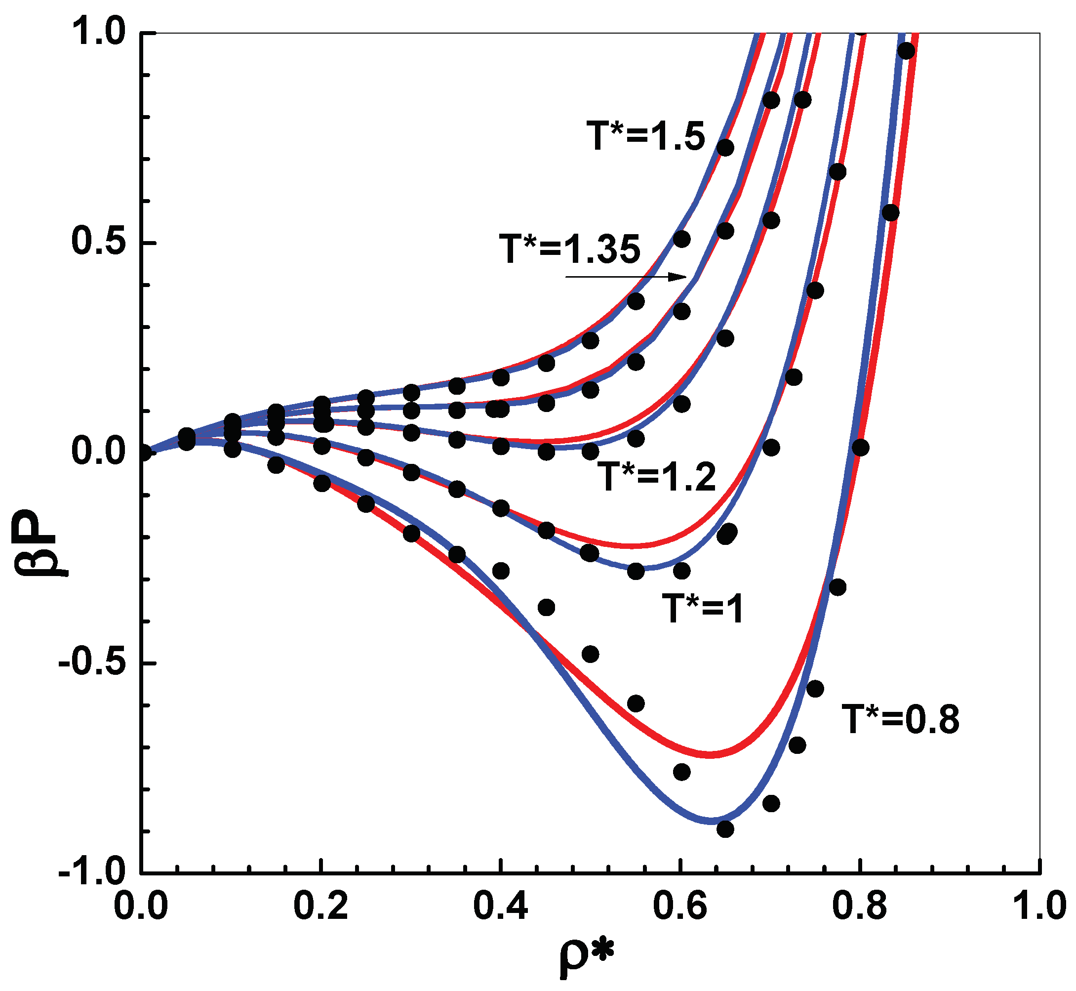
To check the accuracy of CPE, reduced pressure versus reduced density is compared in Figure 4, for different isotherms labeled with , with TMMC simulation data for . As critical temperature obtained in CPE [22] compare well with that from simulations [36], it may be concluded that CPE provides excellent results in the super-critical region ( see isotherms for ). In the spinodal region, the agreement is quite good, except for . Pressure computed via free energy route (blue curves) agree better with data. The differences between CPE results obtained via free energy (blue curves) and compressibility (red curves) routes are indicative of the lack of exact thermodynamic consistency of the MS closure. These results support the view that CPE provides accurate results within the restricted ensemble approach.
8.2. Non-uniform singlet density
Finally, there is an issue within CPE because computed via and will not match in the spinodal region, because the former is negative. As argued below, this is due to the inherent drawback of using a spatially uniform density in that region. It is shown next that the singlet density bifurcates to a non-uniform distribution when . A starting point to show the emergence of this bifurcation is the equation for non-uniform singlet density in a fluid [39]
where , and is the direct correlation function obtained within CPE or any other mean field theories. Being the correlation function in an isotropic fluid, depends only on the radial coordinate r. Here denotes the mean density used in OZE, CPE, mean field theories, etc. Clearly, uniform density, corresponding to the solution of Eq.(65), exits for all . What is to be checked is the emergence of bifurcation to a solution at a spinodal point (see §7.2). For this analysis, and are considered as functions of the arc length parameter ℓ, used for labeling a solution-curve. The slopes and , with respect to arc length ℓ, along the solution-curve, satisfy the equation
where the operator is defined as . The dependence of on is incorporated in . Differentiating once more with ℓ yields
where accounts for second derivative of with . Suppose is a density where bifurcation occurs from solution. At that point on the solution-curve, these equations reduce to
The first equation shows that is a solution where is the eigenvector of corresponding to zero-eigenvalue, and an arbitrary constant. By direct substitution it is verified that is a non-trivial eigenvector, provided , where is the 3D Fourier transform of , and the (radial) Fourier variable. For a non-trivial solution in the second equation, the terms in the square bract must be orthogonal to as is singular. This condition provides a quadratic equitation for , viz.
where denotes Kronecker delta, and is the density-derivative of at . This equation shows that is always a solution, which corresponds to uniform density distribution . However, there is a non-trivial solution when and , where is the density corresponding to a spinodal point. This is given by . Note that and where the subscript denotes density-derivative at . Thus the singlet density bifurcates to a non-uniform distribution at the spinodal points. Although the linear part is singular for , i.e. inside the spinodal region, the bifurcation occurs only at the spinodal points.
For illustrative purposes, consider close to . Then , and so in Eq.(65) may be replaced with . Further, assuming that varies slowly with , so that is approximated by Taylor’s series, Eq.(65) reduces to
where the constants and are the same as in Eq.(5). When is negative, i.e., for within the spinodal region, Eq.(70), together with (say) periodic boundary conditions, will yield oscillatory solutions. Numerical treatment of Eq.(65) will be necessary to establish the occurence of non-trivial in the entire spinodal region.
9. Summary
One of the objectives in this paper is to investigate bifurcation of solutions of OZE and MS closure, applied to full LJ potential, in the gas-liquid co-existence region. This closure yields nearly self consistent results in most part of the phase plane except for low sub-critical temperatures. The method adopted is based on a discrete approximation of OZE in real space. The error reduction factor of algorithm scales as , where is the mesh size. This approach is chosen in lieu of the more conventional approach in Fourier space because Fourier transform of OZE does not exist when . Accurate asymptotic forms of correlation functions, which are essential for the real-space method, are incorporated so that the results are much less sensitive to cutoff length used in the method.
Main findings on bifurcation of solutions are as follows: (i) Spinodal point on the vapor side does not exist on any sub-critical isotherm, although there is a density on a nonphysical solution-branch where inverse compressibility vanishes. (ii) Fold bifurcation points exist on vapor and liquid sides of the isotherm, with a ‘no-real-solution’ region in between. (iii) Spinodal point exists on the liquid branch at a density larger than that of the fold bifurcation point on that side. (iv) In addition, solution-branches (violating the integral condition) with negative compressibility are found on vapor and liquid sides. (v) Complex solutions continuously connect the physical solution-branches (see Figure 3). (vi) It is shown that there are an infinite number of solutions when is negative, which may also be seen as ‘singularity-induced’ bifurcation points. First four observations are quite similar to that found earlier, using real-space methods, for HNC closure [13].
The second objective in the paper is to relate results of CPE, in gas-liquid co-existence region, with those of restricted ensembles. This possibility is corroborated by displaying excellent agreement of pressure-density isotherms with simulation data, where the results show emergence of van der Waals loops in the sub-critical region. Analysis of a simple equation for singlet density distribution shows that it bifurcates to a spatially in-homogeneous distribution at the spinodal points. Perhaps, this is the root cause of all inconsistencies (negative compressibility, van der Waals loops, ‘no-real-solution’ region, etc.) in approaches to OZE in the co-existence region.
References
- J. P. Hansen, I. R. McDonald, Theory of Simple Liquids (Forth Edition) Academic Press, Cambridge. 2013.
- S. V. G. Menon, Bishnupriya Nayak, An equation of state for metals at high temperature and pressure in compressed and expanded volume regions Condensed Matter (MDPI) 4, 2019 , 71.
- C. Caccamo, Integral equation theory description of phase equilibria in classical fluids Physics Reports 274, 1996, 1.
- G. N. Sarkisov, Structure of simple fluid in the vicinity of the critical point: approximate integral equation theory of liquids J. Chem. Phys. 119, 2003, 373.
- N. Choudhury, S. K. Ghosh, Integral equation theory of Lennard-Jones fluids: A modified Verlet bridge function approach J. Chem. Phys. 116, 2002, 8517.
- G. Malescio, P. V. Giaquinta, Y. Rosenfeld, Iterative solutions of integral equations and structural stability of fluids Phys. Rev. E 57, 1998 , R-3723.
- C. A. Stuart, G. Vuillaume, A discrete nonlinear eigenvalue problem with many spurious branches of solutions Z. Anal. ihre Anwend 20, 2001, 183.
- G. Zerah, An efficient Newton’s method for numerical solution of fluid integral equations J. Comp. Phys. 61, 1985, 280.
- L. Belloni, A hypernetted chain study of highly asymmetrical poly-electrolytes Chem. Phys. 99, 1985, 43.
- R. O. Baxter, Method of solution of the Percus-Yevick, Hypernetted-chain or Similar eqautions Phys. Rev. 154, 1967 , 170.
- R. O. Watts, Percus-Yevick equation applied to a Lennard-Jones fluid J. Chem. Phys. 48, 1968, 50.
- L. Belloni, Inability of the hypernetted chain integral equation to exhibit a spinodal line J. Chem. Phys. 98, 1993, 8080.
- J. Kerins, L. E. Scriven, H. Ted Davis, Correlation functions in sub-critical fluid Adv. Chem. Phys. LXV, 1986 , 215.
- K. E. Atkinson, The numerical solution of integral equations on the second kind Cambridge University Press, Cambridge. 2009.
- K. E. Atkinson, L. F. Shampine, Algorithm 876: Solving Fredholm integral equations of the second kind in Matlab ACM Trans. Math. Softw. 34, 2008, 1.
- R. J. F. Leote de Carvalho, R. Evans, D. C. Hoyle, J. R. Henderson, The decay of the pair correlation function in simple fluids: long - versus short-ranged potentials J. Phys.: Condens. Matter 6, 1994, 9275.
- H. B. Keller, Lectures on numerical methods in bifurcation problems (Tata Institute of Fundamental Research) Springer, Berlin, Heidelberg, New York, Tokyo. 1986.
- R. Seydel, Practical Bifurcation and Stability Analysis (Third Edition) Springer, New York, London. 2010.
- M. E. Henderson, H. B. Keller, Complex bifurcation from real paths SIAM J. Appl. Math. 50, 1990, 460.
- A. Sai Venkata Ramana, S. V. G. Menon, Coupling-parameter expansion in thermodynamic perturbation theory Phys. Rev. E 87, 2013, 022101.
- S. V. G. Menon, Scaling of phase diagram and critical point parameters in liquid-vapor phase transition of metallic fluids Condensed Matter (MDPI) 6, 2021 , 6.
- S. V. G. Menon, Convergence of coupling-parameter expansion-based solutions to Ornstein-Zernike equation in liquid state theory Condensed Matter (MDPI) 6, 2021 , 29.
- V. K. Shen, J. R. Errington, Meta-stability and instability in the Lennard-Jones fluid investigated by transition-matrix Monte Carlo J. Phys. Chem. B 108, 2004, 19595.
- N. G. Van Kampen, Condensation of a classical gas with long-range attraction Phys. Rev. 135, 1964 , A362.
- J. D. Weeks, D. Chandler, H. C. Andersen, Role of Repulsive Forces in Determining the Equilibrium Structure of Simple Liquids J. Chem. Phys. 54, 1971, 5237.
- R. O. Baxter, Percus-Yevick equation of hard spheres with surface adhesion J. Chem. Phys. 49, 1968 , 2770.
- Menon, S. V. G.; Manohar, C.; Srinivasa Rao, K. A new interpretation of the sticky hard sphere model J. Chem. Phys. 1991, 95, 9188. [Google Scholar] [CrossRef]
- G. N. Sarkisov, E. Lomba, The gas-liquid phase transition singularities in the framework of the liquid-state integral equation formalism J. Chem. Phys. 122, 2005, 214504.
- A. T. Peplow, R. E. Beardmore, F. Bresme, Algorithms for the computation of solutions of Ornstein-Zernike Equation Phys. Rev. E 74, 2006, 046705.
- D. A. Tikhonov, G. N. Sarkisov, Singularities of solution of the Ornstein-Zernike Equation within the gas-liquid transition region Russian J. Phys. Chem. 74, 2000, 470.
- Waisman, E. The radial distribution function for a fluid of hard spheres at high densities Mean spherical integral equation approach. Mol. Phys. 1973, 25, 45. [Google Scholar] [CrossRef]
- Cummings, P. T.; Smith, E. R. Liquid-gas transition for hard spheres with attractive Yukawa tail interactions. Chem. Phys. 1979, 42, 341. [Google Scholar] [CrossRef]
- V. Venkatasubramanian, Singularity induced bifurcation and the van der pol Oscillator IEEE Trans. Circuits and Systems-I 41, 1994, 765.
- P. A. Monson, P. T. Cummings, Solution of the Percus-Yevick equation in the coexistence region of a simple fluid Int. J. Thermo. Phys. 6, 1985, 573.
- E. Lomba, J. L. López-Martin, On the solutions of the hypernetted chain equation inside the gas-liquid coexistence region J. stat. Phys. 80, 1995, 825.
- J. K. Johnson, J. A. Zollweg, K. E. Gubbins, The Lennard-Jones equation of state revisited Mol. Phys. 78, 1993, 591.
- J. P. Hansen, L. Verlet, Phase transitions of Lennard-Jones system Phys. Rev. 184, 1969, 151.
- L. Mier y Teran, A. H. Falls, L. E. Scriven, H. T. Davis, Structure and thermodynamics of stable, meta-stable, and unstable fluid - Efficient numerical method for solving the equations of equilibrium fluid physics Proc. Eighth Symp. on Thermo-physical Properties 8, 1982 , 45.
- R. Lovett, On the stability of a fluid toward solid formation J. Phys. Chem. 66, 1977, 66, 1225.
Disclaimer/Publisher’s Note: The statements, opinions and data contained in all publications are solely those of the individual author(s) and contributor(s) and not of MDPI and/or the editor(s). MDPI and/or the editor(s) disclaim responsibility for any injury to people or property resulting from any ideas, methods, instructions or products referred to in the content. |
© 2024 by the authors. Licensee MDPI, Basel, Switzerland. This article is an open access article distributed under the terms and conditions of the Creative Commons Attribution (CC BY) license (http://creativecommons.org/licenses/by/4.0/).
Copyright: This open access article is published under a Creative Commons CC BY 4.0 license, which permit the free download, distribution, and reuse, provided that the author and preprint are cited in any reuse.


