Submitted:
12 June 2024
Posted:
13 June 2024
Read the latest preprint version here
Abstract
The Schwarzschild metric encompasses both exterior and interior regions, with a reversal of signature upon transition from one to the other. Inside the Black Hole, the radial spacelike coordinate transforms into a timelike radius, introducing a time-dependent scale factor on the interior metric's angular term. We investigate situating a Black Hole within another, yielding a spherically symmetric vacuum described by the Schwarzschild metric. As the interior metric's angular term contracts towards the center, the inner Black Hole's surface and gravitational field collapse to a point, ultimately vanishing at the singularity. Homogeneously distributing multiple Black Holes inside the shell allows the interior metric's spacelike $t$ coordinate to characterize the expanding space between them and their gravitational fields. Moreover, we propose a cosmological model wherein the intersection of a Universe and Antiverse spawns FRW Universes, transitioning into Schwarzschild Universes as matter aggregates. This mirrors the Black Hole within a Black Hole scenario, with the FRW Universe acting as the shell's surface. Our model is shown to reconcile with cosmological data, explaining the Universe's Dark Energy without a cosmological constant.
Keywords:
cosmology
; black holes
; dark energy
; Schwarzschild metric
1. Introduction
The Schwarzschild metric seems to describe two spacetimes separated by an event horizon. The spacetime outside this horizon is well understood and its predictions have been successfully verified over the past century. The spacetime inside the horizon, commonly treated as the spacetime inside a black hole, has been believed to be unobservable to anyone outside of a black hole since light is not able to cross from inside to outside the horizon. As such, it is believed that the predictions associated with this spacetime are untestable.
When moving from the exterior region to the interior, the signature of the metric is reversed such that the timelike coordinate of the external region becomes spacelike in the interior region and likewise for the spacelike coordinate. This means that the radial spacelike coordinate of the exterior region becomes a timelike radius in the interior. This timelike radius has been interpreted as a time-dependant scale factor on the angular term of the metric in the interior.
In this paper, we place a Black Hole inside a Black Hole. The vacuum between the Black Hole and outer shell in this case is also a spherically symmetric vacuum and therefore must be described by the Schwarzschild metric. The contraction of the angular term of the interior metric as can be understood in this case as causing the inner Black Hole, along with its gravitational field, to contract to a point and vanish at . When we put multiple Black Holes homogeneously and isotropically distributed inside the shell, we can interpret the t coordinate of the interior metric as being the spherically symmetric space between the Black Holes and their gravitational fields.
We present a model of cosmology where the intersection of a Universe/Antiverse pair generates an FRW Universe and Antiverse. This FRW Universe subsequently cools and decays into a Schwarzschild Universe as the matter clumps and we have a situation analogous to the Black Hole inside a Black hole situation where the FRW Universe represents the surface of the shell of the interior metric. This model is compared to cosmological data and it is found that it is capable of accounting for the Dark Energy of the Universe without the need for a cosmological constant.
2. Finite Black Holes Inside an Infinite Black Hole
The interior region of the Schwarzschild metric (Region II in Figure 1) is described by the Schwarzschild metric:
Equation 1 is the interior metric and for the rest of the paper it is important to remember that when discussing the interior metric, t is the spacelike coordinate and r is the timelike coordinate.
The interior metric describes the interior of a Black Hole. If we place a Black Hole inside the interior metric, the vacuum between the Black Hole and the surface of the shell of the interior metric is also a spherically symmetric vacuum. This can be trivially visualized in Figure 2
We can see that the vacuum in Figure 2 is spherically symmetric and therefore must also be described by the Schwarzschild metric.
The radial coordinate r of the interior metric is timelike, so as r goes from u to 0, time moves forward. So the Black Hole at the center of Figure 2 is at some in the interior metric and moves toward in that metric as time passes. A notable feature of the metric in equation 1 is the angular term . This term is multiplied by r which goes from u to 0 as time passes. This means that as the Black Hole falls through time in this metric, it’s surface area will decrease proportionally to r as a consequence of this angular term. At , which is the curvature singularity of the metric, the Black Hole surface area will go to zero, and the Black Hole will no longer exist. It is as though the Black Hole gets squeezed out of existence at the singularity.
If we now imagine that the Black Hole is being orbited by some material, then the contraction of the term will also cause those orbits to be squeezed closer to the surface of the Black Hole as time passes. Figure 3 depicts the relative scale of the gravitational field around the Black Hole as it moves through time toward in the interior metric.
According to the interior metric, the basis vectors get larger as r decreases, becoming infinite at . Therefore, the proper distance/time between t coordinates increases as the system falls to .
Consider Figure 4 which depicts the curvature of the t coordinates in the exterior metric near the surface of a Black Hole. The t coordinate lines are the curved lines and they come from solving the metric for rest observers () and integrating to get the following equation:
Where each line corresponds to a fixed value of t, with being the flat line on the r axis. Vertical worldlines on this coordinate chart are the worldlines of observers at rest and their height is the proper time elapsed. We can see that for a given , less proper time passes for rest observers the closer they are to the horizon. The worldlines of observers falling from two different radii are also shown in Figure 4.
We can conceptualize the t coordinate lines as analogous to isocontours on a contour chart, where represents the highest level and represents the lowest level. The trajectory of a falling observer follows the geodesic of shortest distance from the highest level to the lowest level, ensuring their worldline remains perpendicular to the t coordinate lines at every point. Consequently, the worldlines of all falling observers start vertically at , gradually curving to maintain orthogonality to the t coordinate lines at each point, and eventually becoming horizontal at , .
But if the Black Hole is in the interior metric, then the proper time between t coordinate lines will increase as the system falls to in the interior metric. This has the effect of shifting the gravitational field inward toward the horizon over time as depicted in Figure 5
The solid t-coordinate lines are the t coordinate lines at some reference time in the interior metric. The dotted lines are the t-coordinate lines at some such that those lines are separated by more proper time relative to the solid lines. As shown in Figure 5, this increase in proper distance between coordinate lines shifts the location of a given closer to the horizon. Since is related to the acceleration a rest observer feels at a given distance from the horizon, this tells us that the acceleration field is also squeezed toward the horizon as the Black Hole falls toward in the interior metric.
So while the and terms of the Black Hole system are contracted to a point, the t coordinate far from the Black Hole we placed in the interior metric becomes spacelike and its expansion represents an expansion of space. We can understand this by adding more Black Holes into the shell such that they are distributed homogeneously and isotropically in the infinite space t inside the shell, but separated enough that they do not interact with each other gravitationally. The space between those systems is a vacuum parameterized by the t coordinate of the interior metric.
The equation for a 2D hyperboloid surface embedded in three dimensions is given by:
For our purposes, we will be considering the special case where , which gives the one and two sheeted hyperboloids of revolution. Next, we note the following relationship with regards to the Kruskal-Szekeres coordinates:
Equation 4 appears to be only for one dimension of space, but if we think of X as a radius, then it can describe a 3D isotropic hyperboloid. So comparing to Equation 3, if we set and where R is a radius of a circle in this example, we obtain an equation that matches the form of Equation 3 where :
Equation 5 describes 2D hyperboloid surfaces for a given r where the interior metric has negative . This means that the interior metric describes a 2-sheeted hyperboloid. Note that Figure 1 is for constant and , meaning there exists identical diagrams for each 3D spherical direction.
We will for now focus on region II from Figure 1, where region I captures the external metric and region II captures the interior metric. If we choose some constant value of in the interior metric and plot Equation 5 for the interior metric, we get the surfaces shown in Figure 6.
We see we have two separate sheets, but for the moment, we will only focus on the top sheet. The meaning of the bottom sheet will be discussed in Section 4.
Light cones in Figure 6 are oriented vertically and light travels on 45 degree lines. If we choose any point on the surface and project a past and future light cone from that point. We can move that point to the apex of the surface (at ) by hyperbolically rotating the spacetime until the point is at the apex. We can do this without changing anything in the spacetime because the hyperbolic rotation is a translation in t, and is Killing vector of the manifold. When the point is rotated to the apex, we see then that the light cone is symmetric relative to the surface left and right and into and out of the page. This symmetry means the spacelike foliations of the interior metric’s vacuum are isotropic and homogeneous.
This can be extended to three spatial dimensions by allowing R to be the radius of a 3D sphere. In this formulation, we put ourselves at and the circles on the surfaces in Figure 6 will become spheres that are isotropic and homogeneous in space and inhomogeneous in time, which is consistent with the Cosmological Principle.
So the surface of Figure 6 represents the vacuum of the interior metric with nothing (not even another Black Hole) inside of it. There are no intrinsic spacelike spherical features in this vacuum, and so on its own, it describes a homogeneous space that expands over time (this will be discussed in more detail in Section 3). But when we place black holes in this spacetime, they create spacelike spherical regions in the vacuum that contract over time as has been discussed.
We can depict Black Holes inside the interior metric and better understand their contraction over time with Figure 7.
Figure 7 is a modified picture of region II from the Kruskal-Szekeres coordinate chart in Figure 1 with the dark hyperbolas represent the singularity at , the 45 degree dashed lines represent the surface of the interior metric, and the hyperbolas between those are the interior vacuum at some with three black holes shown as wells stretching out from this hyperbola. The undeformed hyperbola where the wells are is shown as a dotted line for reference.
So we see from the figure that the gravitational wells created by Black Holes can be understood as the spacelike hypersurface in the interior spacetime being locally stretched back to the surface of the interior spacetime. Since is a Killing vector of the spacetime, we can apply hyperbolic rotations to the hyperbola to make any of the Black Holes on the surface centered on the diagram (i.e. there is no difference between the three Black Holes in the figure because we can hyperbolically rotate any of them to the center of the diagram). The relative sizes of the wells are related to the relative Schwarzschild radii of each Black Hole.
The wells stretch out to the surface on the interior region because, as shown in Appendix A, the event horizon of the exterior metric can always be hyperbolically rotated to . So it is important to keep in mind that the tips of the wells of the Black Holes represent the event horizon of the exterior solution, not the singularity.
The left side of Figure 7 shows the vacuum with three Black Holes at some time and the right side shows the same surface at a later time . As the surface moves up toward , the wells close. This is the contraction of the gravitational field discussed earlier. As the surface moves to , the wells close completely and the spacelike surface becomes completely flat and empty. So the contraction of the and terms of the internal metric lead to a contraction of the wells and the expansion of the term results in the expansion of the space between the different wells.
A notable point here is that the entire surface, including the wells, represent an interior hypersurface at some r. The meaning of this will be expanded on in Section 3, but we should note that as we change the value r of the hypersurface, the relative positions of the wells can change and new wells can be formed at different times (i.e. the hypersurface at some may have no wells, whereas the same surface at some later time can have a well on it if, for instance, a gravitational collapse occurred at some time in between). In fact, we can say that two gravitating systems will combine if they move together more quickly than the t-vacuum between them expands.
Furthermore, we can think of gravitational wells of non-Black Holes, such as a star, as being indents in the hypersurface that do not reach back to the interior surface at a sharp point, those are just smooth, shallower dips in the surface.
It is interesting to think about the interplay of space and time from these gravitational wells. The surface without a Black Hole is perpendicular to the time dimension r in the interior metric. But the gravitational wells stretch that surface in the r direction. Thus, the r direction of the interior region gains spacelike characteristics in the gravitational wells because the spacelike surface gets deformed in the r direction. This is why the r coordinate is timelike in the interior vacuum and spacelike in the exterior vacuum. It also creates a connection between the ’up’ and ’down’ directions of gravity that come from the exterior metric, and ’future’ and ’past’ from the interior metric. In this model, ’up’ and ’future’ are the same direction on the manifold, where when we observe this direction from the exterior metric point of view, we see the direction as spacelike and when we observe it from the interior metric point of view, we see it as timelike. The same is true for the ’down’/’past’ direction.
We will explore what occurs at the event horizon of the gravitational wells in Section 4, but first we will look at this model in the context of the cosmology of the Universe.
3. The Interior Metric as a Model of Cosmology
The interior metric describes a situation where the volume of the space of the vacuum is zero when (because the term is zero there), expands over time, and becomes infinite at . This bears a striking resemblance to the Big Bang model of cosmology where the Universe started in an infinitely dense state and subsequently expanded and cooled, condensing into galaxies and gravitational clusters forming a cosmic web surrounding spherically symmetric vacuums of space.
The FRW metric of cosmology describes a perfect fluid with uniform pressure and matter density throughout space which expands over time. This is an adequate description of the Universe in early times when the entire Universe was a hot plasma with uniform density and pressure. But after recombination, The pressure and density of the Universe was no longer uniform. Matter began to clump together into structures creating areas of high and low pressure/density.
We can model cosmology as being described by the FRW metric in the pre-recombination era, but after recombination, the Universe is governed by the Schwarzschild metric. The CMB represents a surface r just inside the shell of the interior Schwarzschild metric, which is a uniform surface that is seen as a surface a the same constant time, regardless of the time r from which it is observed. As will be shown, modelling the Universe in this way will help us resolve the Dark Energy problem without the need for a cosmological constant. This is because the expansion of the t dimension of the interior metric follows a pattern of infinite initial expansion, followed by a period of slowing expansion, followed again by a period of accelerated expansion. This accelerated expansion accounts for the dark energy without the need for a cosmological constant.
If we consider a filament in the cosmic web, which is where most of the matter is but is still mostly vacuum, we can think of the filament as a cylinder that will get stretched along its length and squeezed radially over time. In other words, the cosmic web can be understood as the ongoing ’spagghetification’ of the matter in the Universe as it falls toward the singularity at . Furthermore, the contraction of the term which puts an inward pressure on the gravitating systems may account for the dark matter observations, but this is left as an area for future research.
Let us now compare the Schwarzschild cosmological model to cosmological data to show that the model is in very good agreement with experiment.
3.1. The Scale Factor
Expressions for the proper time interval along lines of constant t and and the proper distance interval along hyperbolas of constant r and from Equation 1 are:
And the coordinate speed of light is given by:
Where a is the scale factor (because t is the spatial coordinate and r is the time coordinate and therefore Equation 6 describes how the proper distance between two points separated by coordinate distance evolves over time). First we should notice that none of the three equations depend on the t coordinate. This is good because the t coordinate marks the position of other galaxies relative to ours. Since all galaxies are freefalling in time inertially, the particular position of any one galaxy should not matter. The proper temporal velocity, proper distance, and coordinate speed of light only depend on the cosmological time r.
A plot of the scale factor vs. r (with ) is given in Figure 8 below:
3.2. The Co-Moving Observer
Let us take a co-moving observer somewhere in the Universe we label as as the origin of an inertial reference frame. We can draw a line through the center of the reference frame that extends infinitely in both directions radially outward. This line will correspond to fixed angular coordinates (). There are infinitely many such lines, but since we have an isotropic, spherically symmetric Universe, we only need to analyze this model along one of these lines, and the result will be the same for any line.
We must determine the paths of co-moving observers ( in the spacetime. For this we need the geodesic equations for the interior Schwarzschild metric [1] given in Equation 1. In these equations u represents a time constant (in Figure 1, the value of u is 1). The following equations are the geodesic equations of the interior metric for t and r) for :
Looking at points , then by inspection of Equation 9 it is clear that an inertial observer at rest at t will remain at rest at t ( if ).
Let us next demonstrate how the interior metric fits with existing cosmological data and calculate various cosmological parameters using that data.
3.3. Calculation of Cosmological Parameters
In order to compare this model to cosmological data, we must solve for u and find our current position in time () in the model. Reference [2] gives us transition redshift values ranging from to , depending on the model used. We can use the expression for the scale factor in Equation 6 to get the expression for cosmological redshift from some emitter at r measured by an observer at [1]:
Furthermore, the deceleration parameter is given by:
By setting Equation 12 equal to zero, we can solve for . With this and equation 6, we can calculate the scale factor at the Universe’s transition from decelerating to accelerating expansion :
Using Equations 11, 13, and the transition redshift estimate, we can get an expression for the present scale factor:
Next, we find expressions for u and our current radius by noting that light from the CMB has been travelling for roughly 13.8 billion years of coordinate time r. Therefore, we can set and use Equations 6 and 14 to obtain the following for u and :
Next we compute the CMB scale factor () and coordinate time () in this model where the redshift of the CMB () is currently measured to be 1100:
We can next derive the Hubble parameter equation using the scale factor. The Hubble parameter is given by (in units of ):
Table 1 below gives the values of u, , , , , , and given the upper and lower bounds of from [2] as well as the 0.75 transition redshift value and assuming . All times are in and is in .
From the results in Table 1, we see that the true transition redshift is likely close to 0.75 given the fact that the current value of the Hubble constant is known to be near 71.6. Thus, more accurate measurements of the transition redshift are needed to increase the confidence of this model, but the 0.75 transition redshift is in fact a prediction of the model and we will see this when it is compared to astronomical data later in this section.
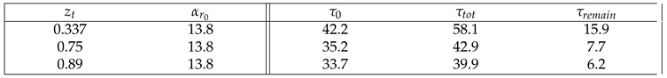
Table 2 has the proper times from to the current time for co-moving observers () by integrating Equation 1. The column gives the time from to . The expression for turns out to be quite simple:
In Table 2 below, the column gives the time between and .
Note that the proper time of the current age of the Universe is actually much larger than the coordinate time . And even though we are presently only about halfway through the “coordinate life” of the Universe (according to Table 1), the amount of proper time remaining is actually much less than the amount of proper time that has already passed (according to Table 2). This provides a measurable prediction from the model: as telescopes such as the JWST peer farther into the past with greater accuracy, we should expect to find stars, galaxies, and structures that are much older than expected because of the increased amount of proper time available for such things to form in the early Universe. Hints of this has already been found with the star HD 140283, whose age is estimated to be nearly the age of the Universe itself [3].
Next we would like to use the u and values found to compare the model to measured supernova and quasar data. First we need to find r as a function of redshift. We can do this by solving for r in Equation 11:
We can derive the expression for t vs. r along a null geodesic where the geodesic ends at the current time and by setting in Equation 1 and integrating:
Next we substitute Equation 21 into Equation 22 to get coordinate distance in terms of redshift:
We need to convert the distance from Equation 23 to the distance modulus, , which is defined as:
Where in Equation 24 is the luminosity distance. Luminosity distance is inversely proportional to brightness B via the relationship:
The brightness is affected by two things. First, the spatial expansion will effectively increase the distance between two objects at fixed co-moving distance from each other. This will reduce the brightness by a factor of (because the distance in Equation 25 is squared). But there is also a brightening effect caused by the acceleration in the time dimension. We define as the temporal velocity of the inertial observer at some r and the speed of light at that r as . The ratio of these velocities gives us:
Equation 26 tells us how far a photon travels over a given period of time measured by the inertial observer’s clock. So we see that as light travels from the emitter to the receiver, this speed decreases. This decrease in the speed from emitter to receiver will result in an increased photon density at the receiver relative to the emitter, increasing the brightness. Therefore, this effect will increase the brightness by a factor of:
This effect is not accounted for in the current relativistic cosmological models and therefore gives a second prediction that light from the distant Universe should appear brighter than expected.
Taking these brightness effects into account, the total brightness will be reduced by an overall factor of relative to the case of an emitter and receiver at rest relative to each other in flat spacetime. Equation 25 in terms of co-moving distance t and redshift z becomes:
Giving the luminosity distance as a function of co-moving distance t and redshift z:
Which gives us the final expression for the distance modulus as a function of co-moving distance and redshift:
A plot of distance modulus vs. redshift is shown in Figure 9 below plotted over data obtained from the Supernova Cosmology Project [4]. A Curve calculated from the row in Table 1 is plotted as this value provides the best fit for the data.
Figure 10 shows the same curve from Figure 9 for the Hubble diagram plotted out to higher redshifts with the quasar data from [5] also shown with error bars.
Figure 11 is a comparison of the CDM model with the Schwarzschild model with the transition redshift. As can be seen in this figure, both models are in very close agreement for the range of data available.
3.4. Behavior of Light in the Interior Metric
The path of light should also be affected by the angular term of the interior metric. When light is gravitationally lensed, its momentum vector changes direction, meaning it gains a non-zero . We can see the precise behaviour of lensed light by looking at the geodesic equation for angular motion [1] (we will examine the case for planar rotation where ).
For light, we will use . If we consider light lensed by a galaxy, as the light passes the galaxy at some coordinate time , it will have some angular velocity and initial angle as it leaves the galaxy. It is currently assumed that the light then continues along a straight line as it leaves the gravitational field, but as we shall see, this is not the case. The would be the angle caused only by the gravitational lensing, without any additional effects from the cosmological model (i.e. the angle we would expect when only taking into account the mass of the galaxy). Given these initial conditions, the solution to Equation 31 is:
Both the bracketed expression and will always be negative (because is negative and ) such that the second term is always positive. Therefore, the observed lensing angle will be increased by the amount as a result of this effect (where r is the coordinate time at which the light is observed). Furthermore, since for the light increases over time, the will correspondingly decrease as well and the result of this is that the increase in lensing angle over time will also result in a redshift of the light relative to unlensed light.
We see that the ’excess angle’ is dependant on the lensing rate . So if we consider two cases where in one case, the light is gently lensed over a large distance/time by some angle and in the other case, light is lensed by a more dense mass the same , the lensing rate would be higher in the second case relative to the first. So even though the pure gravitational lensing angle would be the same in both cases, the observed angle would be greater in the second case because the lensing rate would be greater in that case.
4. The Antiverse at the Beginning of Time
We have to this point shown that the cosmological model of the Universe can be described as an FRW Universe which subsequently condenses into a Schwarzschild spacetime as described in the current work. But we must now consider the source of the initial FRW Universe.
Figure 13 shows the full Schwarzschild metric in Kruskal-Szekeres coordinates. The diagram can be split in two along the diagonal where in the top right half, forward time points up in both the interior and external regions while in the bottom left half, forward in time points down. The direction of positive space is also swapped when looking at the upper and lower halves. For the external metric, the radius increases to the right in the upper half and to the left in the lower half. For the interior metric, the spatial t coordinate goes from to from left to right in the upper half and from right to left in the lower half.
We can therefore conjecture that the diagram is describing both a Universe expanding up from the center and an Antiverse expanding down from the center, each one moving toward a singularity. We expect that the Antiverse is made of mostly anti-matter because the directions of both time and space are reversed relative to each other and therefore we expect the particles of the second Universe to have opposite charges relative to the first. This interpretation provides a resolution to the question of why we only tend to see matter in our Universe. It is because the equivalent amount of antimatter is contained in this mirror Universe. The lower hyperboloid sheet in Figure 6 therefore represents a 2D slice of the Anitverse at a given time. Thus, the pair of Universes satisfies CPT symmetry.
So we can think of the source of the Universe as being the intersection of the Universe and Anitverse. This intersection represents a pair production of Universe and Antiverse moving in positive and negative time. The intersection is a point of infinite energy and temperature, like an engine generating the FRW Universe and Antiverse which each condense into their respective Schwarzschild Universe and Antiverse. This intersection would be represented by the point in Figure 13.
In Figure 7, we showed the gravitational wells of Black Holes stretching back to this intersection point. We can imagine an identical picture mirrored in the horizontal axis representing the same situation in the Antiverse. Therefore, when a particle reaches an event horizon, it meets its antiparticle and annihilates with it. The light from this annihilation would then decompose back into matter and anti-matter particles that would begin falling again from into their respective Universe and Antiverse.
Putting all this together, we can think of the surface of the interior metric as a source of infinite energy at infinite temperature where the Universe and Antiverse intersect. Matter ’evaporates’ from this surface, creating a fog we know as an FRW Universe. This fog subsequently cools and condenses into stars and galaxies analogous to clouds. In some regions, the matter in these clouds become so dense, the matter there falls back to the surface via the gravitational wells analogous to rain falling from the clouds. The matter then evaporates once again, starting the process over. So we can think of the Universe as a heat engine operating within an infinite temperature differential powered by the intersection of the Universe and Antiverse.
Acknowledgments
All data generated or analysed during this study are included in this published article [and its supplementary information files
Conflicts of Interest
There are no competing interests
Appendix A. Length Contraction in Kruskal-Szekeres Coordinates
The Kruskal-Szekeres coordinates are the maximally extended coordinates for the Schwarzschild metric. The coordinate definitions and metric in Kruskal-Szekeres coordinates are given below (derivation of the coordinate definitions and metric can be found in reference [1] where and ).
With the full metric in Kruskal-Szekeres coordinates given by:
The coordinate chart for this metric is given in Figure 1. Light-like geodesics are 45 degree lines on this diagram. Let us take the differentials of T and X in equations A1:
Calculating the partial derivatives, rearranging and defining we get:
Next, we need to calculate from equations A4 by factoring out from each equation and dividing:
Next, we make the following definition:
This is the derivative of the rest frame at t since plugging into equation A5, we get .
Now consider the hyperbolas of constant r in region I of Figure 1 which represent the worldlines of rest observers in Kruskal-Szekeres coordinates. In these coordinates, rest observers accelerate over time as evidenced by the fact that their worldlines are hyperbolas in these coordinates. If we consider the X position of a rest observer at some , we see that its X-coordinate is given by where is the X coordinate of the rest observer at r when . At , the rest observer is moving with some velocity relative to itself at on this coordinate chart. Therefore, we should expect that the X coordinate will be length contracted as t increases in the rest frame in Kruskal-Szekeres coordinates. The length contracted value of X in the rest frame at r and is given by:
Where is the effective velocity of the rest observer in Kruskal-Szekeres coordinates as defined in equation A6.
So even though the X coordinate grows for an observer at rest in the Kruskal-Szekeres coordinate chart, when we shift to the frame of the rest observer by taking into account the length contraction of the Kruskal-Szekeres coordinates in that frame, we see that we end up back at . This means that the surface of the event horizon of a Black Hole can always be shifted to on the Kruskal-Szekeres coordinate chart by taking length contraction into account. This amounts to hyperbolically rotating the spacetime such that the ’present’ is always at on the coordinate chart.
Appendix B. CMB Temperature and Absolute Simultaneity
The Minkowski spacetime of Special Relativity has no intrinsic geometric features that can be used for reference. Since it is everywhere and at all times uniform, one cannot define a universal ’present’ in Special Relativity, leading to the relativity of simultaneity. To put it more precisely, it is not possible for causally disconnected observers in Special Relativity to synchronize their clocks.
But the Schwarzschild geometry does have intrinsic geometrical features. Importantly, the intrinsically spherical nature of time in the interior metric provides causally disconnected observers the ability to synchronize their clocks by agreeing ahead of time to start their clocks when they are at a specific r (in the interior metric). This allows us to order events absolutely regardless of their spacetime separation because each event occurs at a specific r and the r of different events can be used to objectively order the events in time.
In our Universe, this amounts to agreeing to start the clocks when the CMB monopole is at a specific temperature. This works because the CMB temperature is related to the scale factor a of the Universe, which itself is a function of r.
Since r is not itself directly measurable, it is more useful in a practical sense to use the temperature of the Universe as a measure of cosmological time. The CMB is a perfect black body and its temperature is inversely proportional to the scale factor a. We can relate them precisely with:
Where T and a are the CMB monopole temperature and scale factor at any time r and and are the temperature and scale factor at some reference time . To keep the equations simple, we can choose the reference scale factor to be 1 and use a temperature scale such that the CMB monopole temperature at that time is also 1. In Section 3, it was shown that the current scale factor is very close to 1 and the current CMB monopole temperature is 2.725K. Therefore, if we measure temperature in units of Kelvin divided by 2.725, we get a unitless temperature scale and the relationship between T and r becomes
and
Furthermore, we have an estimate for u from Section 3 of 27.3. If we work in units of time where (such that one of these units of time equals 27.3), then we can also drop the u from the equations (so we are working with a unitless timescale).
Taking the derivative of equation A10, we obtain:
Substituting equations A9 and A11 into equation 1 we get the metric as a function of CMB monopole temperature T:
In these coordinates, as and as . So by using the CMB monopole temperature as a measure of cosmological time, we get a clearer understanding of time dilation. We can establish a universal rest frame in the Schwarzschild metric (the co-moving observer for whom the CMB has only a monopole), against which we can measure all motion. The velocity of a frame relative to the co-moving frame can be determined by the CMB dipole observable in that frame. Therefore, the CMB dipole seen in a given frame tells that frame its absolute velocity. This absolute velocity is not only increased motion through space relative to the co-moving observer, but also increased motion through time. A reference frame with a non-zero velocity will see the CMB monopole cool more quickly according to their clock relative to the co-moving observer as a result of the time dilation. So we can describe time dilation between two frames in our Universe as the difference in the rate at which the CMB monopole cools (or heats up in the collapsing Universe) according to the clock in each frame. A moving frame is not only moving faster through space than the co-moving observer, but also faster through cosmological time measured using the CMB monopole temperature.
Therefore, time dilation is better thought of as one frame moving faster through cosmological time than another, rather than one frame’s clock ’ticking more slowly’ than the other. And, in the author’s opinion, using the CMB monopole temperature as the measure of cosmological time allows for a more intuitive description of the time dilation.
References
- Carroll, S.M. Lecture Notes on General Relativity, 1997, [arXiv:gr-qc/9712019v1].
- Lima, J.A.S.; Jesus, J.F.; Santos, R.C.; Gill, M.S.S. Is the transition redshift a new cosmological number? 2014, [arXiv:astro-ph.CO/1205.4688]. arXiv:astro-ph.CO/1205.4688].
- Bond, H.E.; Nelan, E.P.; VandenBerg, D.A.; Schaefer, G.H.; Harmer, D. HD 140283: A STAR IN THE SOLAR NEIGHBORHOOD THAT FORMED SHORTLY AFTER THE BIG BANG. The Astrophysical Journal 2013, 765, L12. [Google Scholar] [CrossRef]
- Project, S.C. Supernova Cosmology Project - Union2.1 Compilation Magnitude vs. Redshift Table (for your own cosmology fitter). http://supernova.lbl.gov/Union/figures/SCPUnion2.1 mu vs z.txt, 2010. Accessed on Aug. 17, 2017.
- Risaliti, G.; Lusso, E. Cosmological constraints from the Hubble diagram of quasars at high redshifts, 2018, [arXiv:astro-ph.CO/1811.02590]. arXiv:astro-ph.CO/1811.02590].
Figure 1.
Kruskal-Szekeres Coordinate Chart
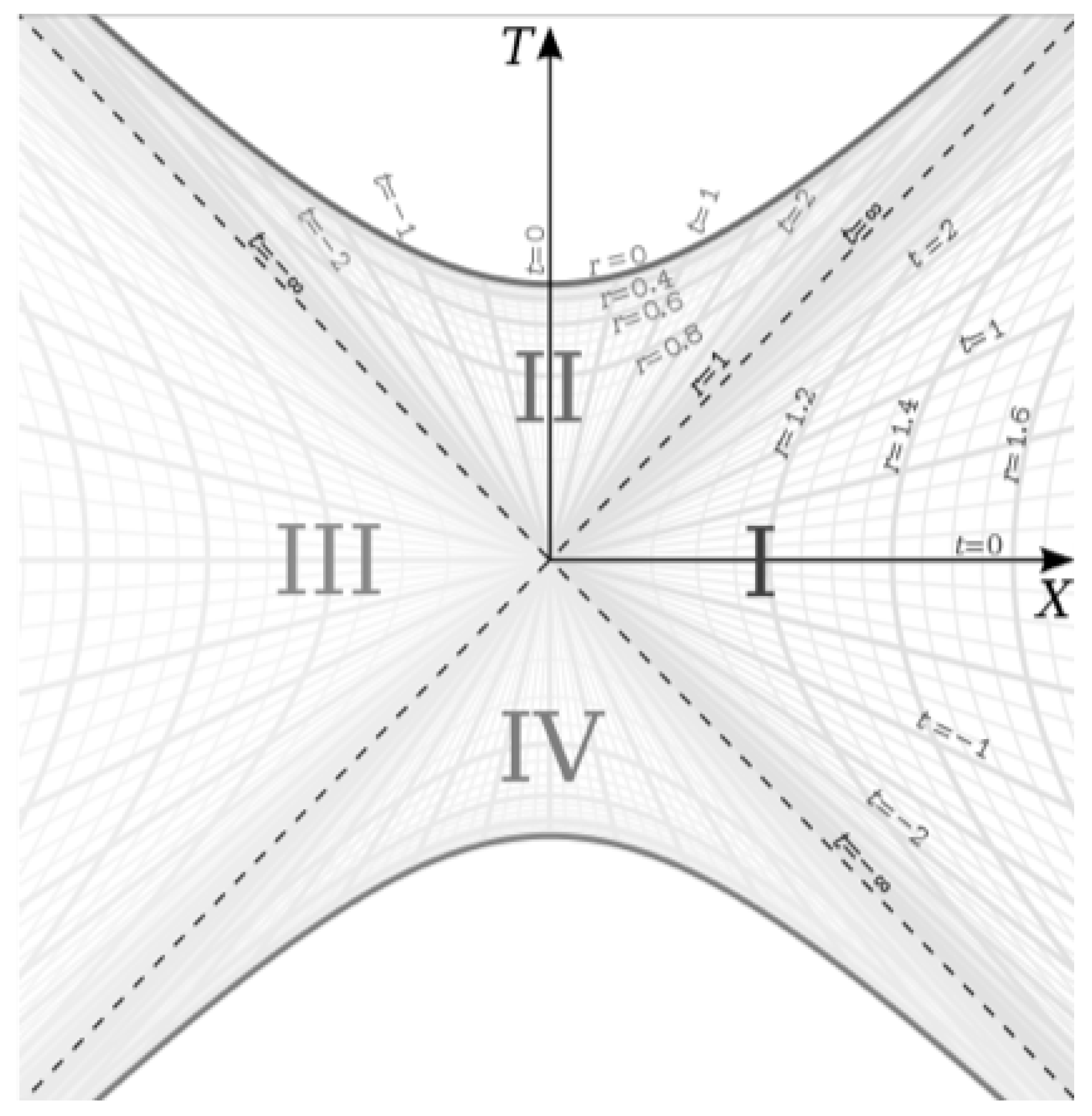
Figure 2.
Black Hole inside of a Black Hole
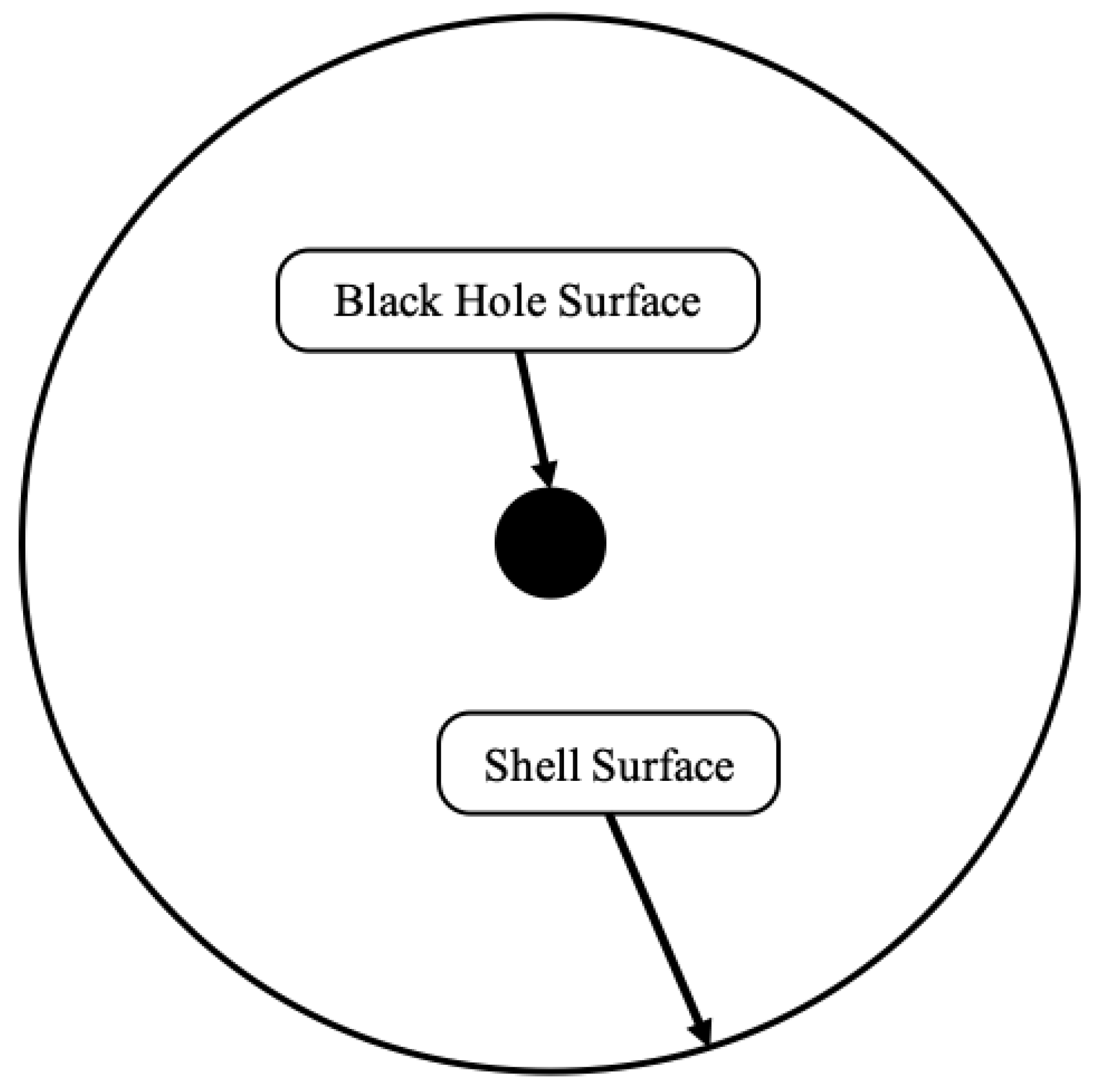
Figure 3.
Contraction of a Spherical Gravitational Field and its Orbits in the Interior Metric
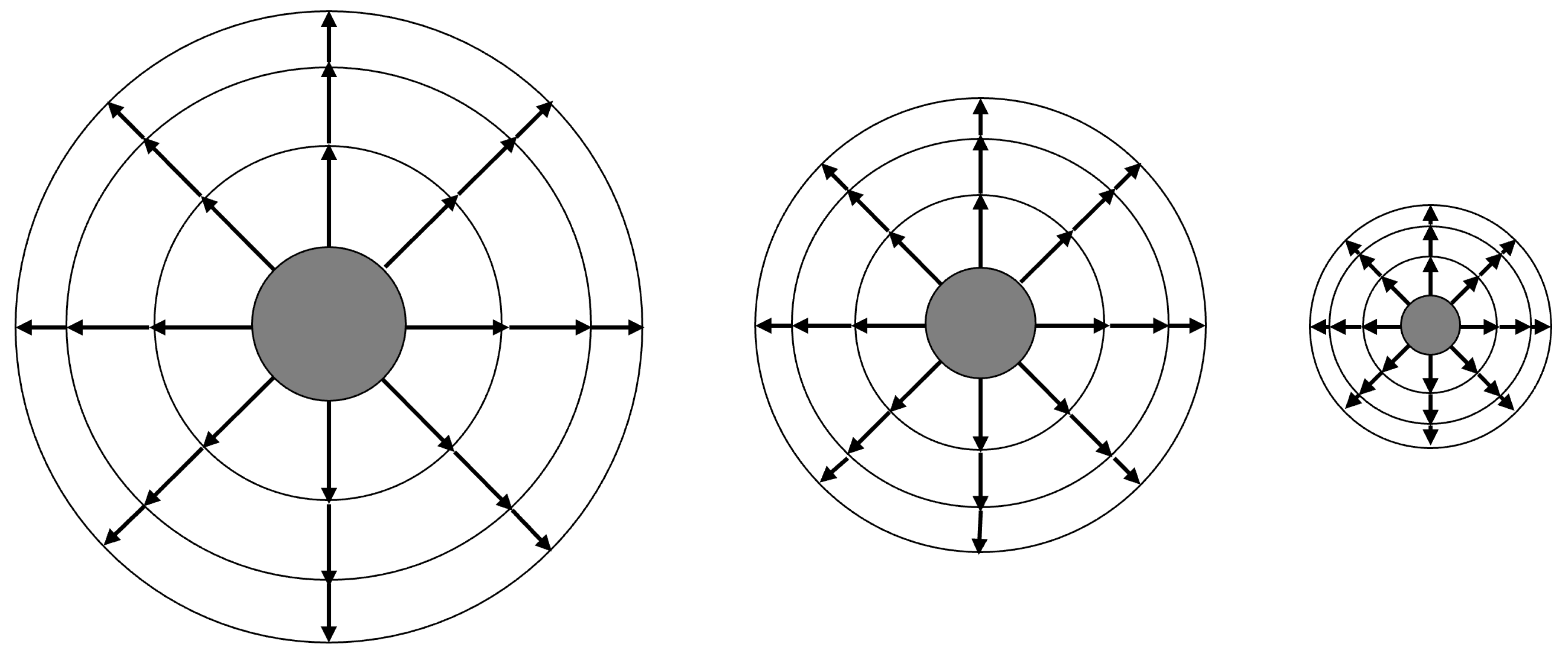
Figure 4.
Falling Worldlines on the Modified Schwarzschild Coordinate Chart
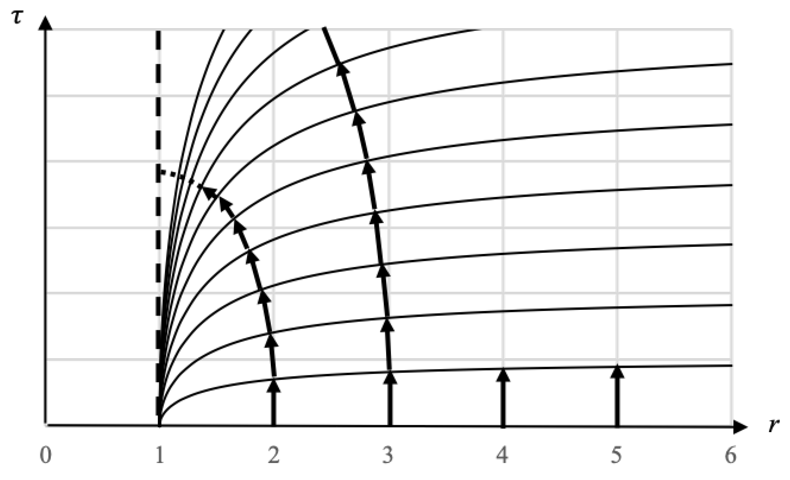
Figure 5.
The Shifting of the Gravitational Field from the t Coordinate Expansion

Figure 6.
2D Surfaces of Constant r for the interior Metric
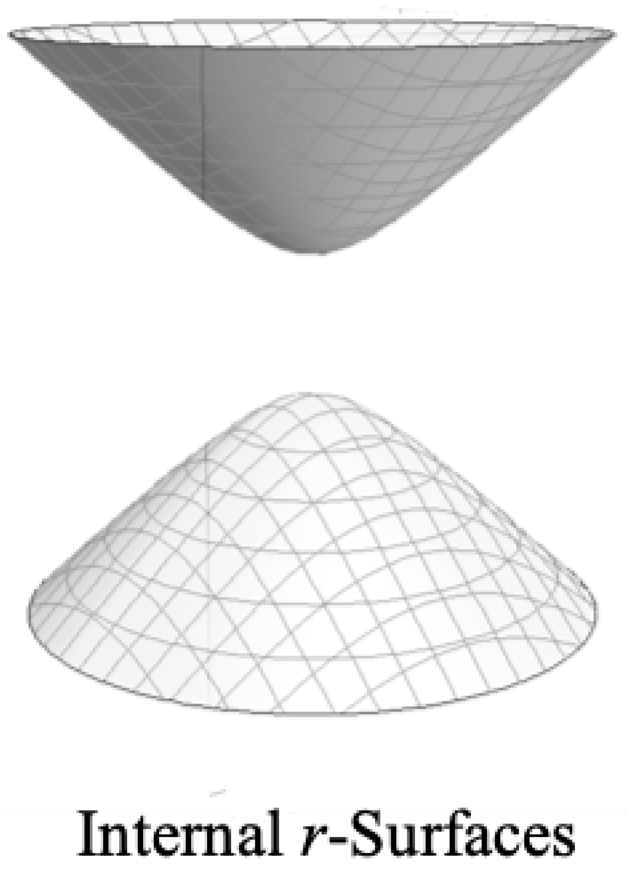
Figure 7.
1-D Visualization of the Distortion of the Interior Vacuum Manifold by Black Holes
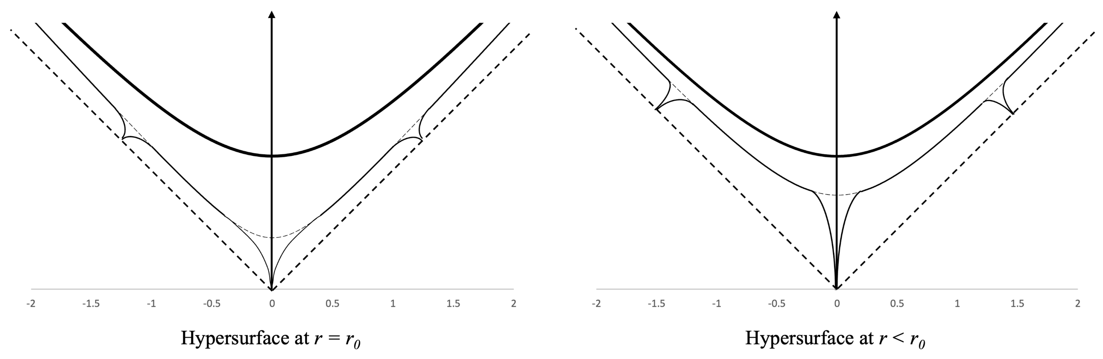
Figure 8.
Scale Factor vs. r for
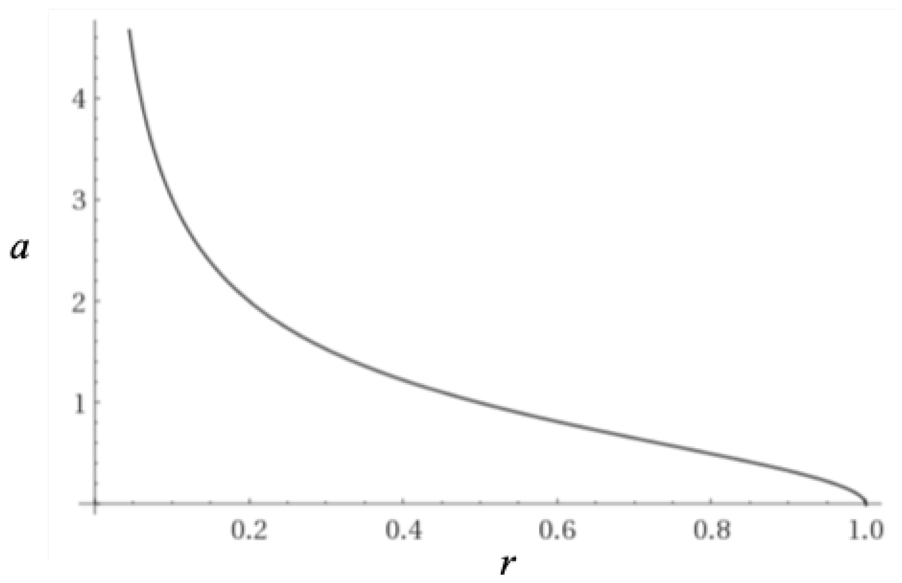
Figure 9.
Distance Modulus vs. Redshift Plotted with Supernova Measurements
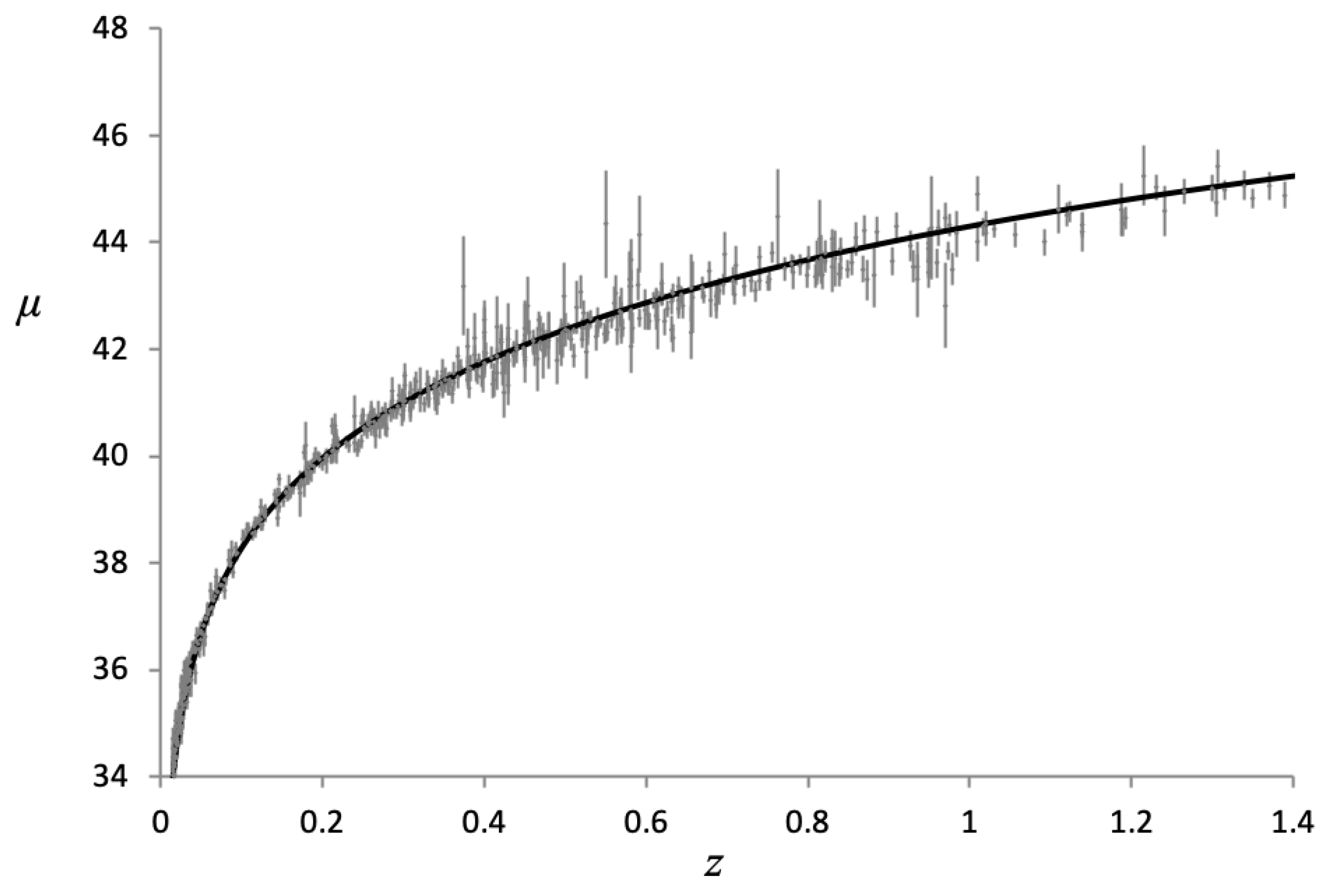
Figure 10.
Distance Modulus vs. Redshift Plotted with Quasar Measurements
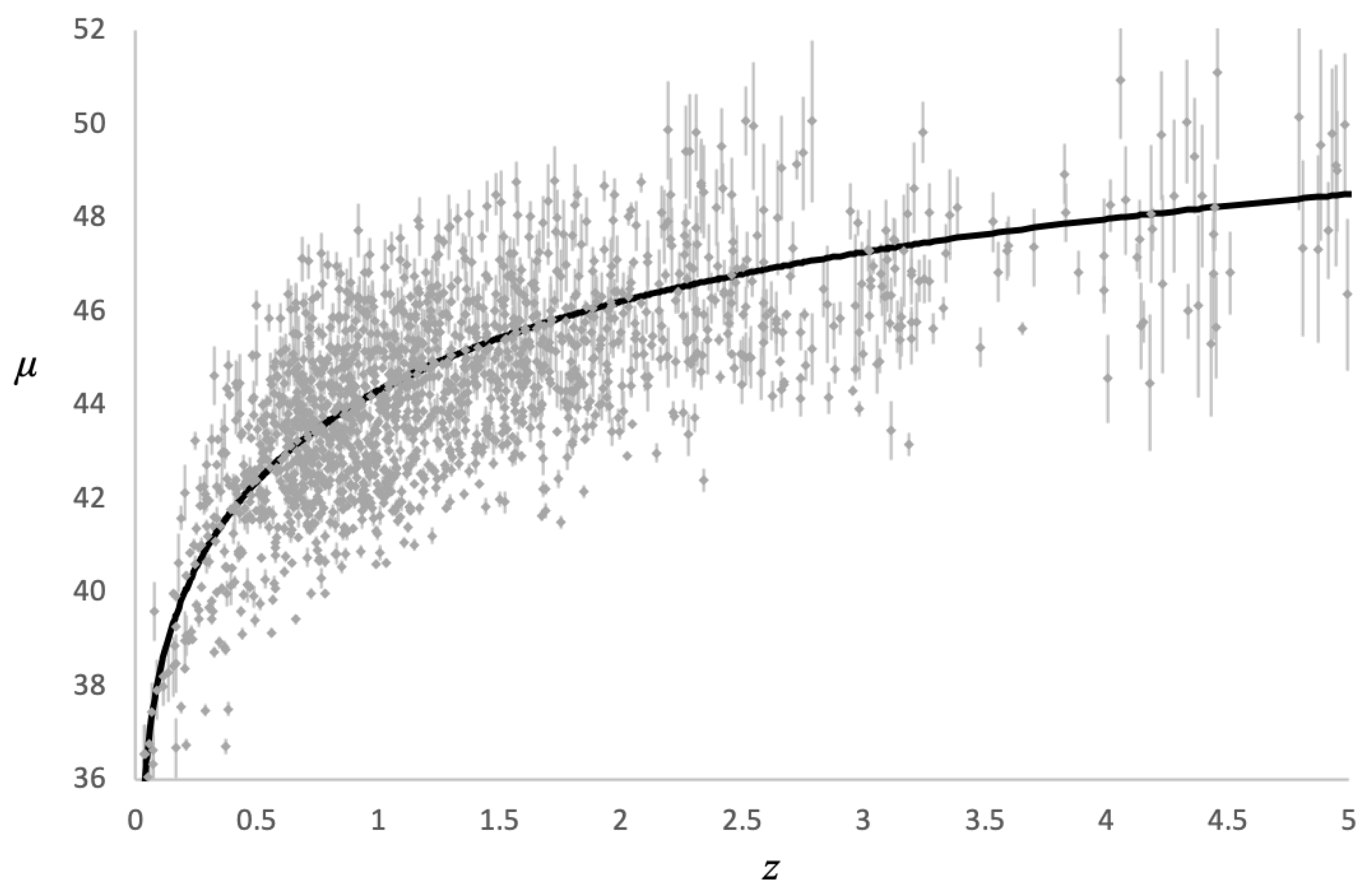
Figure 11.
Distance Modulus vs. Redshift Comparison with CDM
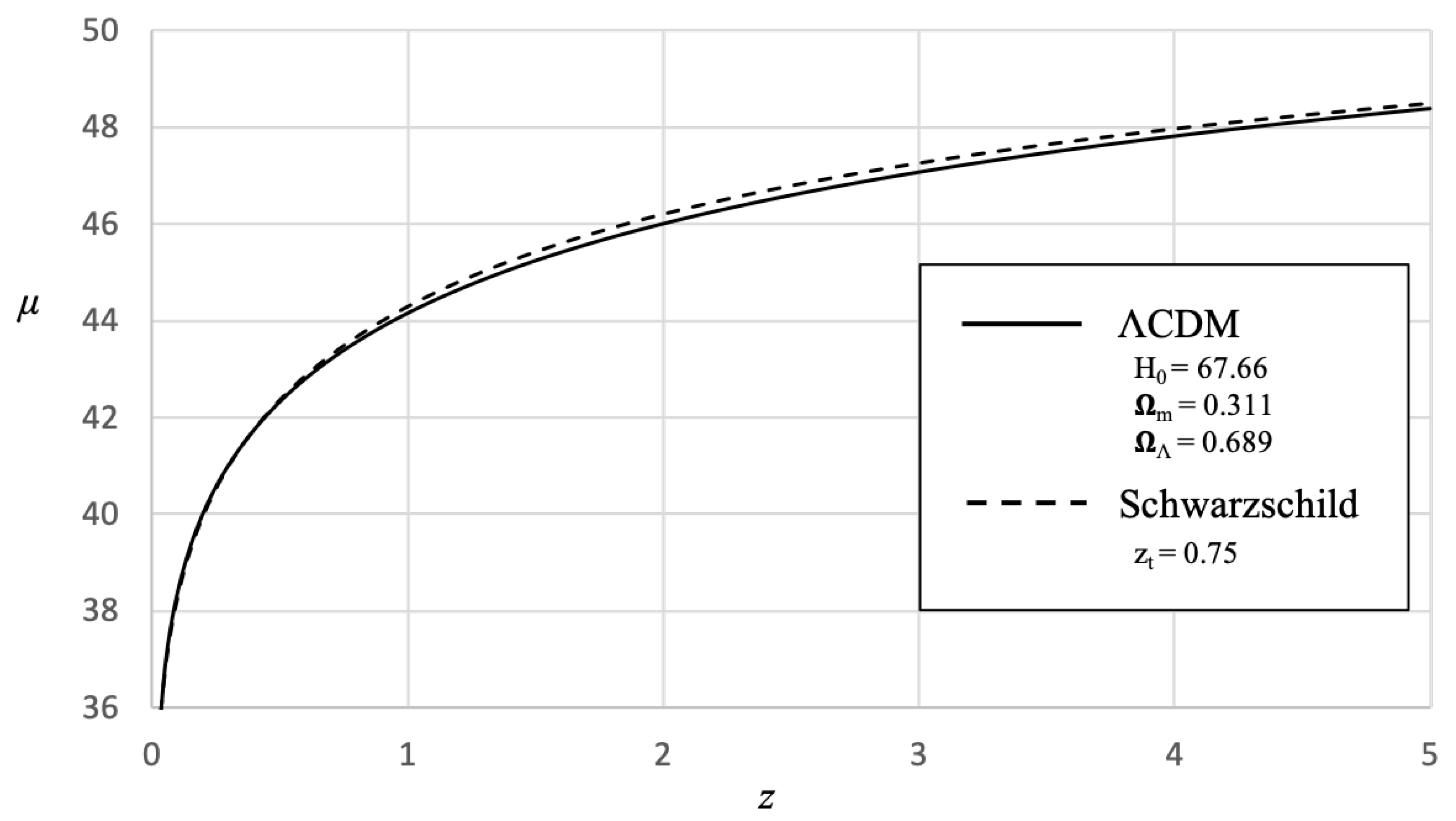
Figure 12.
Lookback Time vs. Redshift
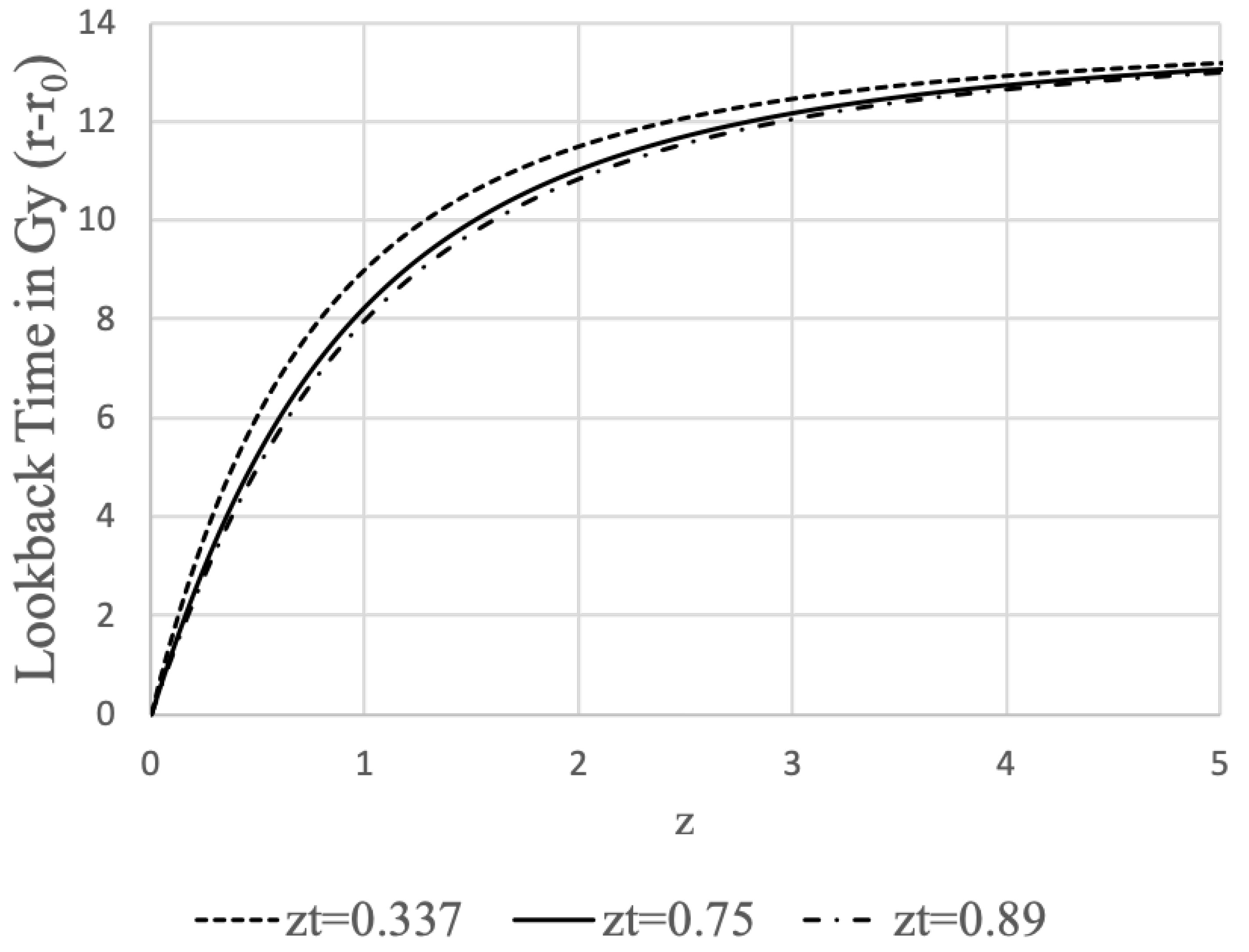
Figure 13.
Universe and Antiverse
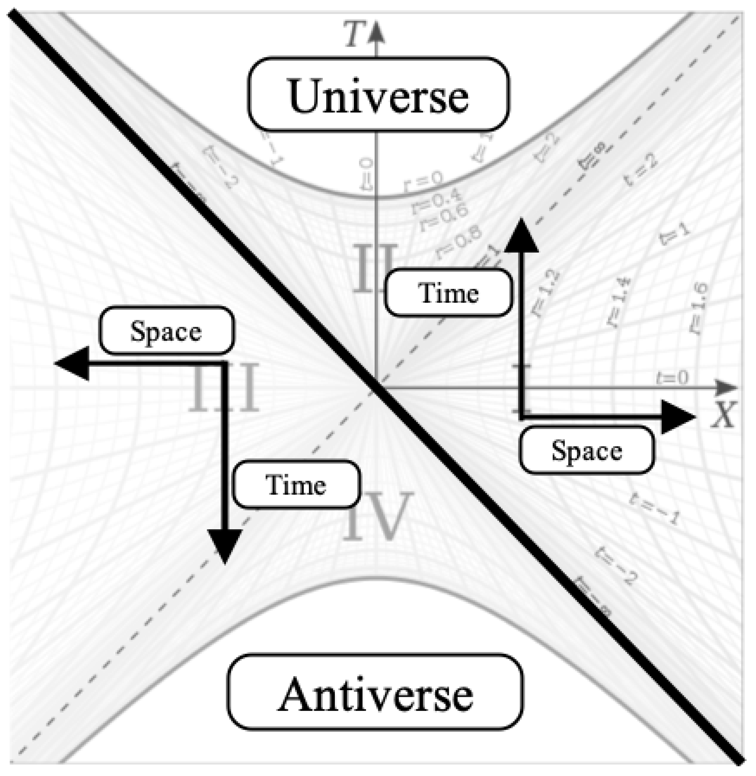

Table 1.
Limiting Cosmological Parameter Values Based on Measurement and a 13.8 Gy Age of the Universe
Table 1.
Limiting Cosmological Parameter Values Based on Measurement and a 13.8 Gy Age of the Universe
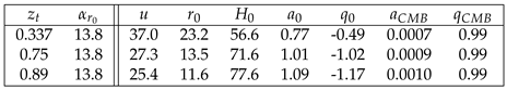
Table 2.
Limiting Proper Times Based on Measurements and an age of 13.8 Gy for the Universe (Time is in Gy)
Table 2.
Limiting Proper Times Based on Measurements and an age of 13.8 Gy for the Universe (Time is in Gy)
Disclaimer/Publisher’s Note: The statements, opinions and data contained in all publications are solely those of the individual author(s) and contributor(s) and not of MDPI and/or the editor(s). MDPI and/or the editor(s) disclaim responsibility for any injury to people or property resulting from any ideas, methods, instructions or products referred to in the content. |
© 2024 by the authors. Licensee MDPI, Basel, Switzerland. This article is an open access article distributed under the terms and conditions of the Creative Commons Attribution (CC BY) license (http://creativecommons.org/licenses/by/4.0/).
Copyright: This open access article is published under a Creative Commons CC BY 4.0 license, which permit the free download, distribution, and reuse, provided that the author and preprint are cited in any reuse.


